EFFECTS OF LAMINAR BOUNDARY LAYER

ON A MODEL BROAD-CRESTED WEIR

lITJ,

no. ~ ~

/,

£/19111by

3MK9UK

11111111111111111111111111111111111111111111111111111111111111II3 4067 01204475 5

TA1.U4956NO.28ENGIN GEN

CIVIL ENGINEERING RESEARCH REPORTS

This report is one of a continuing series of Research Reports published bythe Department of Civil Engineering at the University of Queensland. ThisDepartment also publishes a continuing series of Bulletins. Lists of recentlypublished titles in both of these series are provided inside the back cover ofthis report. Requests for copies of any of these documents should be addressedto the Departmental Secretary.

The interpretations and opinions expressed herein are solely those of theauthor(s). Considerable care has been taken to ensure the accuracy of thematerial presented. Nevertheless, responsibility' for the use of this materialrests with the user.

Department of Civil Engineering,University of Queensland,St Lucia, Q 4067, Australia,[Tel:(07) 377-3342, Telex:UNIVQLD AA4031Sj

L. T. ISAACS, BE, MEngSc, PhD, MIE Aust.

Senior Lecturer in Civil Engineering

~SEARCH REPORT NO. CE 28

Department of Civil Engineering

University of Queensland

September, 1981

Synopsis

This report describes an approximate method

for the analysis of flow with a laminar boundary

layer over a ~odel hroad-crested weir. The method

has been used to demonstrate the effects of the

laminar boundary layer and the results have shown

that these effects are significant. If the energy

is calculated from depth and discharge measurements,

large energy losses appear to occur at low flow

rates in laboratory experiments. Losses real and

apparent, are explained and the methods presented

may be used to estimate the correct energy values.

CONTENTS

Page

1.

1. INTRODUCTION

1.1 Flow Over a Model Broad-crested Weir

The flow over a model broad-crested weir (Figure 1)

is often studied in undergraduate laboratory classes because

If q is the two-dimensional discharge and y the

depth, provided the velocity is uniform over a cross-section,

the specific energy, E, is given by

1.

2.

3.

4.

INTRODUCTION

1.1 Flow over a Model Broad-crested Weir

1.2 Objective of the Investigation

METHOD OF SOLUTION

2.1 Calculation of Depth and Velocity

2.2 Boundary Layer Calculations

2.3 Solution Procedure

RESULTS

FINITE ELE~mNT ANALYSIS FOR VELOCITIES

1

1

6

6

7

9

11

12

-15

(i)

(ii)

(iii)

prototypes of these weirs are commonly used as

flow measuring devices,

subcritical, critical and supercritical flow

can be observed, and

the experiment affords an opportunity for the

demonstration and application of the Specific

Energy concept.

5. CONCLUSION

APPENDIX A

APPENDIX B

NOTATIONS

REFERENCES

j)e.~'(!r~' )~~~

18

19

20

E Y + L (la)2gy2

y + V2(lb)

2g

in which g is the acceleration due to gravity and V is the

velocity.

If there are no losses and the bed level upstream

and downstream of the weir are the same (see Figure' 1) ,

in which w is the level of the weir sill relative to the

upstream bed level.

E1

E2

E3

E - W1

(2)

(3)

2.

(4)

(5)

made, e.g. in the

discharge and depth

,of no energy losses

1.5 YcE·2

3.

The broad-crested weir experiment is done in our

laboratory in a channel 250 rom wide constructed with glass

sides and perspex bottom. The model weir has the profile shown

in Figure 1 and detailed in Table 1. The sill is 64 rom above

the channel bed which is horizontal. Discharge is measured

with a weighing tank and depths are measured by pointer gauges

with verniers marked in gradations of 0.2 rom. The specific

energy at a cross-section is determined by Equation lao Over

the range of flows used, the measured depths at station 3

lie between 3 and 30 rom. Some difficulty occurs in the

measurement of depth because of the presence of capillary

waves, and at the low flows the experimental error is relatively

large. Consequently, there is a wide scatter in the experimental

results for low flow rates but, in general, the results

indicate that there are substantial losses at low flows and

that the relative losses decrease as the flow rate increases.

Some experimental results obtained by the writer are plotted

in Figure 2. In Figure 2 and in some later figures, Yc is

chosen for the independent variable rather than q because Yc

gives a more convenient scale. The effects of a change of

± 0.1 rom in the measured depths at station 3 have been computed

for some values and are shown by the vertical bars through

these values and by the plot of percentage change in E3/E 1

slope along MNPR (Figure 1), the assumption

between sections 1 and 3 would generally be

calculation of depth at section 3 given the

at section 1.

Flow is assumed to occur at critical depth over the

weir. Hence,

in which Yc = (q2 g)V3 is the critical depth and Ec is the

critical or minimum specific energy for the discharge q. If

the bed is smooth and there are no discontinuities in the

)

~

H~

&~w~00WHUI~maH~

mN H

W>a

~~

~

~

~p~H~

:1 1, .

~I

3(em)

2Yc

1

~o

5.

ee.....<:)

c..-e ,..,

....>0­U.I,C:

rri-U.I G.I 4c:c::n.- c:QleIc::n.c:c: U

~ 2U

II.

4.

I

I•

•

I

0,8

1,0

0,9

....UJ<,,..,UJ 07,

FIGURE 3 Effect of a small change in Y3 on E 3/E 1

2 3Yc (em)

4 5 presented in Figure 3. The calculated value of E is very

sensitive to the value for y in the supercritical region,

particularly if the Froude No., F, is high since

FIGURE 2 Experimental values of E3/E 1as a function of Yc I - F2 (6)

Conversely, the value of y must be insensitive to the value

for E used in supercritical regions and the neglect of any

losses when the depth is calculated is justifiable. Problems

arise when the specific energy in the supercritical region is

required and it is not surprising that students' results have

a wide variation, especially for the lower flow rates. However,

-..

6. 7.

there is a general trend apparent and an investigation was

done to determine if the general trend could be explained by

the presence of a laminar boundary layer.

The objective of the study described in this report

was the development of an approximate analysis to demonstrate

the effects of the laminar boundary layer and to estimate the

magnitude of these effects for the laboratory experiment.

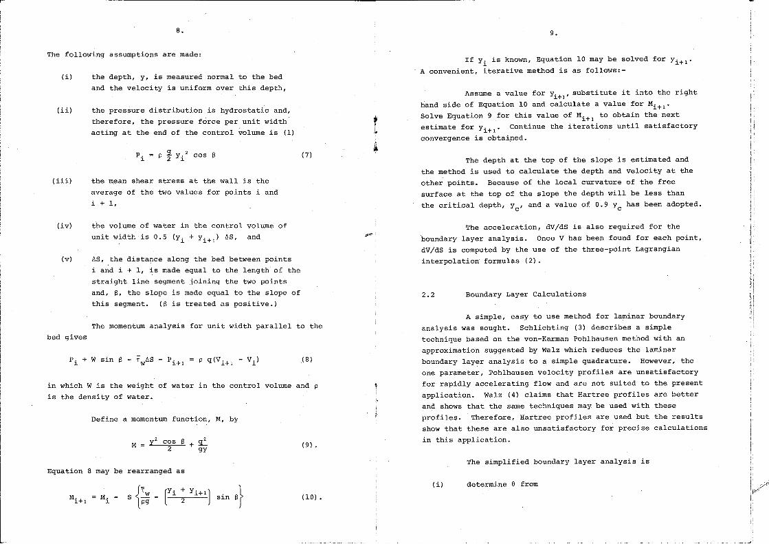
Control volume for momentum analysis

Calculation of Depth and Velocity

FIGURE 4

flow•

2.1

If i and i + 1 are two points on the slope and the

depth, Yi' is known at i, the depth, Yi+l' at i + 1 is found

from a momentum analysis. The control volume used is shown in

Figure 4.

For the purposes of an approximate analysis the flow

over the weir sill is assumed to occur at critical depth and

critical velocity. A preliminary estimate based on the results

for a laminar boundary layer on a smooth flat plate showed

that the energy losses along the sill are very small and they

have been neglected in the analysis. The following method was

developed for the calculation of depth and velocity down the

slope, N - P, and along the horizontal bed, P - R (Figure 1)

for a known discharge.

The profile is described by a number of points at

which x,the horizontal distance, and z, the height of the bed

above datum are specified. In the analysis, values for TW

are

. also specified at these points.

Objective of the Investigation

METHOD OF SOLUTION

1.2

2.

This objective has been achieved. An approximate

method for the analysis of the effects of the laminar boundary

layer which gives results consistent with the observed pattern

has been developed. However, because of the assumptions and

approximations used in the analysis, the method cannot be

expected to yield an'ac~urate, quantitative result.

The effects of the laminar boundary layer are often

important in hydraulic model studies at small scales, e.g. in

model testing of dam spillways. The method described in this

paper may be readily adapted and used to obtain an estimate

of these effects. Furthermore, the work done indicates that

the general method used is satisfactory and could form the

basis for the development of an accurate method for quantitative

assessments.

The solution involves the calculation of the variation

of depth and velocity along the weir sill, M - N, and down the

slope, N - R, (Figure 1) and the calculation of the values of

momentum thickness, a, displacement thickness, 0*, and the

shear stress along the bed, TW'

from a boundary layer analysis.

Since the velocity depends on TW

and the boundary layer analyais

on the velocity, an iterative approach is necessary.

B.

The following assumptions are made:

9.

2.2 Boundary Layer Calculations

The depth at the top of the slope is estimated and

the method is used to calculate the depth and velocity at the

other points. Because of the local curvature of the free

surface at the top of the slope the depth will be less than

the c r i.t.Lca l, depth, Yc'

and a value of 0.9 Yc has been adopted.

Assume a value for Yi +1

' substitute it into the right

hand side of Equation 10 and calculate a value for Mi+ 1 •

Solve Equation 9 for this value of Mi +1

to obtain the next

estimate for Yi+l' Continue the iterations until satisfactory

convergence is obtained.

If Yi is known, Equation 10 may be solved for Yi+l'

A convenient, iterative method is as follows:-

The acceleration, dV/dS is also required for the

'boundary layer analysis. Once V has been found for each point,

dV/dS is computed by the use of the three-point Lagrangian

interpolation formulas (2).

(7)

~S, ,the distance along the bed between points

i and i + 1, is made equal to the length of the

straight line segment joining the two points

and, S, the slope is made equal to the slope of

this segment. (S is treated as positive.)

the volume of water in the control volume of

unit width 'is 0.5 (Yi + Yi+l) ~S, and

the mean shear stress at the wall is the

average of the two values for points i and

i + 1,

(i) the depth, y, is measured normal to the bed

and the velocity is uniform over this depth,

(v)

(ii) the pressure distribution is hydrostatic and,

therefore, the pressure force per unit width

acting at the end of the control volume is (1)

(iv)

(iii)

in which W is the weight of water in the control volume and p

is the density of water.

The momentum analysis for unit width parallel to theA simple, easy to use method for laminar boundary

analysis was sought. Schlichting (3) describes a simple

technique based on the von-Karman Pohlhausen method with an

approximation suggested by Walz which reduces the laminar

boundary layer analysis to a simple quadrature. However, the

one parameter, Pohlhausen velocity profiles are unsatisfactory

for rapidly accelerating flow and are not suited to the present

application. Walz (4) claims that Hartree profiles are better

and shows that the same techniques may be used with these

profiles. Therefore, Hartree profiles are used but the results

show that these are also unsatisfactory for precise calculations

in this application.

(B)

(9) •y2 cos S + L2 gyM

Define a momentum function, M, by

bed gives

Equation B may be rearranged asThe simplified boundary layer analysis is

(10) •

(i) determine e from

10. 11.

dV/dS is found from the velocity variation previously computed

(Section 2.1).

in which V = V(S) is the velocity external to the boundary

layer, v = ~/p is the kinematic viscosity (~ is the viscosity)

andS =: 0 where 82V/v = 0, a = 0.441 and b = 4.165 for Hartree

profiles (4). weir profileTABLE 1

x z Comments(m) (m)

- 0.390 0.0640 point M

0.000 0.0640 point N

0.015 0.0631

. 0.030 0.0617

0.080 0.0521

0.130 0.0424

0.180 0.0327

0.230 0.0231

0.~80 0.0134

0.330 0.0038

0.350 0.0011

0.370 0.0000 point P

0.520 0.0000 point R

(iv) determine 6*

Since the displacement thickness is required only

along the section PR (Figure 1) where dV/dS is close to zero,

a value of 6*/8 = 2.6, from the results for a flat plate,

is used for the calculation of 6* from 8 at points along PRo

1J

(11)

(12)

a(f) and hence the wall

~ dVv dSr

determine the parameter a

(ii) calculate the profile shape parameter,f,

(iii)

The integral may be evaluated by numerical quadrature.

In the present study S = 0 was assumed at the upstream end of

the sill, the contribution to the integral from the flow along

the sill is V b 2 (where 2 is the length of the sill) and thectrapezoidal rule was used to evaluate the integral down the slope.

shear stress, TW'

~ V a-8- (13) 2.3 Solution Procedure

a and f values are tabulated in Walz (4). Intermediate values

may be found by linear interpolation.

For accelerating flows, f varies between 0.0 and

0.1082 and a varies between 0.2212 and 0.3922. In the present

study, values for f considerably larger than the allowable maximum

were calculated at the top of the slope. Where this occurred,

the value of 0.3922 was used for a.

For any given two-dimensional discharge, q, the

critical depth, Yc' and the critical velocity, Vc' are calculated

and assumed to apply along the sill. The contribution to the

integral in Equation 11 from the boundary layer along the sill

is evaluated. The ·flow and boundary layer growth down the

slope and along the bed downstream of the slope are calculated

by an iterative procedure as follows:-

Because a simple, approximate analysis is required,

the estimate for a given above has been adopted. The approximation

does, however, mean that the results obtained are open to question

and should not be used for other than preliminary estimates.

(i)

(ii)

assume TW

values for all specified points

(T w = 0 is an acceptable assumption),

calculate depths, velocities and accelerations

(Section 2.1),

12.13.

3. RESULTS

Iteration 1Iterotionb

,.;:::::::::-- --"~

\~ initial.\~\ assumption

/

1,5

2,0

E toI-----j~-----­<,:z

with values for V and dV/dS from (ii) calculate eand T

Wat the specified points (Section 2.2).

As a check of the method for velocities (Section 2.1), -3 2 1 )an analysis was carried out for q = 3.132 x 10 m /s (Yc = 0.0 m

with T = 0 and y = 0.01 m at the top of the slope. The specificw

energy calculated for flow between P and R (Figure 1) from the

computed depth and velocity was 79.6 mm which was less than 1%

different from the exact value of 79.0 mm.

The method was applied to the model broad-crested weir

64 mm high ~ith the profile given in Table 1.

The calculations may be done manually with the use

of graphs and an electronic calculator but they are tedious

and time consuming. The method can be readily programmed

for a computer and this is recommended if a number of cases

are to be studied.

Repeat (ii) and (iii) until satisfactory convergence

is obtained. About four iterations, are usually sufficient.

(iii)

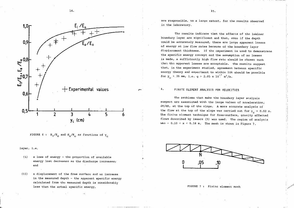
The plots of E~/Eo and Ea/Eo are consistent with the

pattern observed in the laboratory. The experimental results

obtained by the author for this report lie within the two

curves and it appears that the two effects of the boundary

depth plus the displacement thickness is an estimate of the

depth that would be measured by a pointer gauge. The apparent

specific energy, Ea, is the specific energy calculated from

Equation la when Ya is used. E~/Eo and Ea/Eo are plotted as

functions of the critical depth, Yc' in Figure 6. The

experimental values for E /E are also plotted in Figuve 6.3 1

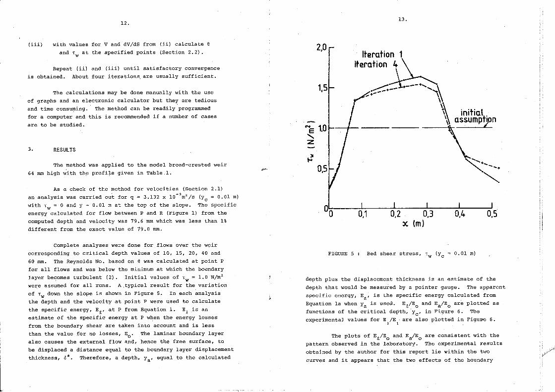
Complete analyses were done for flows over the weir

corresponding to critical depth values of 10, 15, 20, 40 and

60 mm. The Reynolds No. based on e was calculated at point P

for all flows and was below the minimum at which the boundary

layer becomes turbulent (2). Initial values of T = 1.ON/m2, w

were assumed for all runs. A ,typical result for the variation

of T down the slope is shown in Figure 5. In each analysisw

the depth and the velocity at point P were used to calculate

the specific energy, E~, at P from Equation 1. E~is an

estimate of the specific energy at P when the energy losses

from the boundary shear are taken into account and is less

than the value for no losses, Eo. The laminar boundary layer

also causes the external flow and, hence the free surface, to

be displaced a distance equal to the boundary layer displacement

thickness, c*. Therefore, a depth, y , equal to the calculateda ,

FIGURE 5 Bed shear stress, TW (Yc 0.01 m)

14. 15.

FINITE ELEMENT ANALYSIS FOR VELOCITIES

are responsible, to a large extent, for the results observed

in the laboratory.

The results indicate that the effects of the laminar

boundary layer are significant and that, even if the depth

could be accurately measured, there are large apparent losses

of energy at low flow rates because of the boundary layer

displacement thickness. If the experiment is used to demonstrate

the specific energy concept and the assumption of no losses

is made, a sufficiently high flow rate should be chosen such

that the apparent losses are acceptable. The results suggest

that, in the experiment studied, agreement between specific

energy theory and experiment to within 10% should be possible-2 2for Yc >. 35 rom, Le. q > 2 .•05 x 10 m Is.

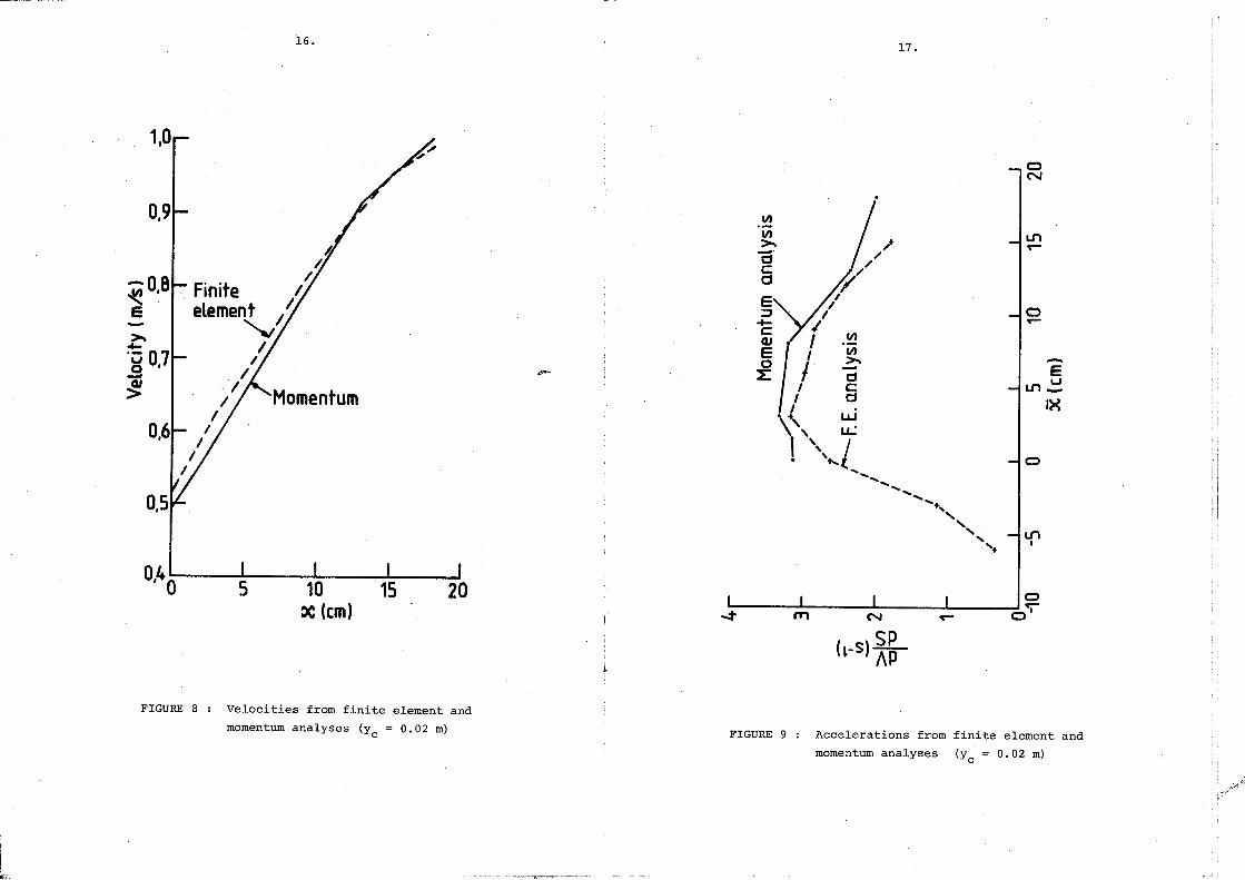
The problems that make the boundary layer analysis

suspect are associated with the large values of acceleration,

dV/dS, at the top of the slope. A more accurate analysis of

the flow at the top of the slope was carried out for Yc = 0.02 m.

The finite element technique for free-surface, gravity affected

flows described by Isaacs (5) was used. The region of analysis

was - 0.10 < x < 0.18 m. The mesh is shown in Figure 7.

·4.

3Yt (em)

-t- Experimental values

21

+

0,5L..---L-.__-'--_---L__---'-__...£.-_--'

tVI.LJ

00,8I.LJ<,

FIGURE 6

layer, Le.

(i)

(ii)

a loss of energy - the proportion of available

energy lost decreases as the discharge increases;

and

a displacement of the free surface and an increase

in the measured depth - the apparent specific energy

calculated from the measured depth is considerably

less than the actual specific energy,

oI

FIGURE 7

,10I

Finite element mesh

16. 17.

1,0

>...'u 0,7.9~

0,6

Finite

II)

II)>.-a0

c:aE::J..c:OJeo~

oN

-eLn~

IX

o

LnI

oL---_~ ...I_ ...L.. _:::!'Cj""

o

SP(~-S) AP

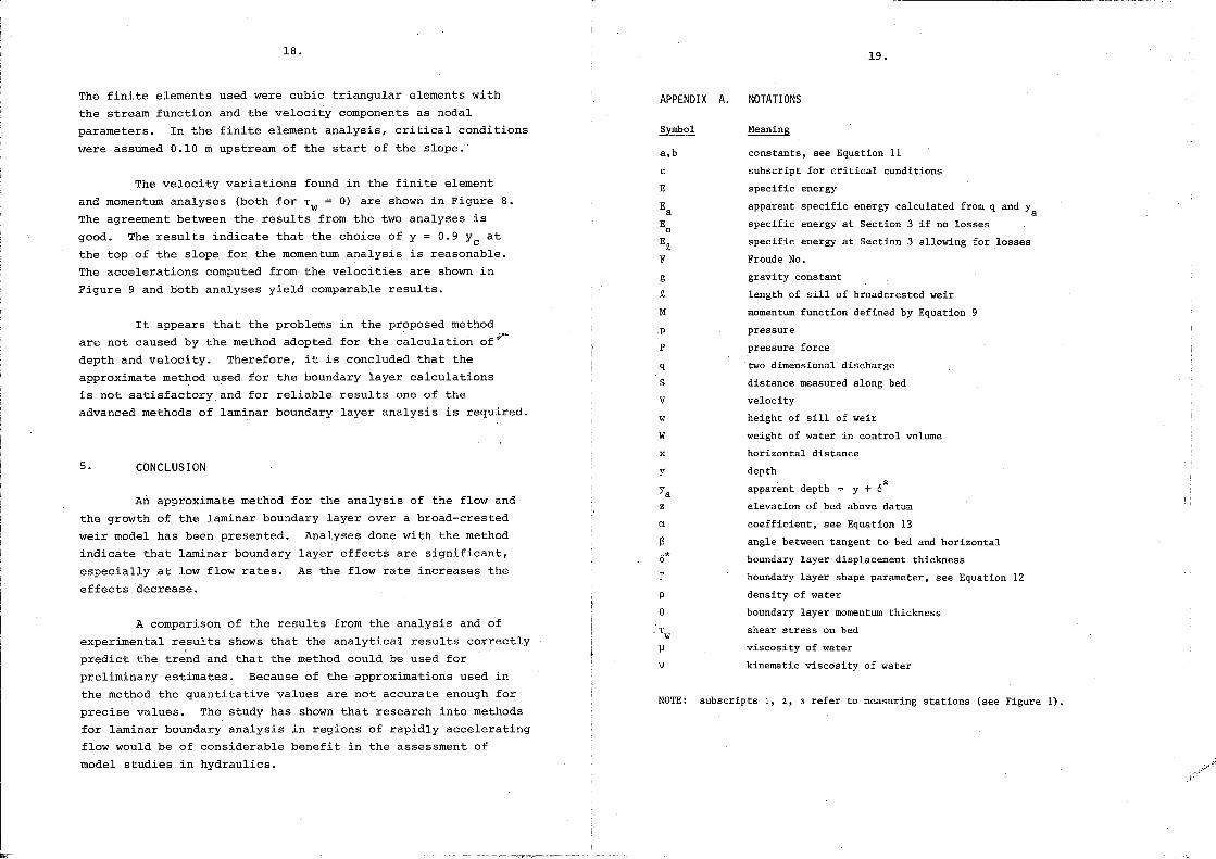
FIGURE 8 velocities from finite element and

momentum analyses (Yc = 0.02 m) FIGURE 9 Accelerations from finite element and

momentum analyses (Yc = 0.02 m)

APPENDIX A.

18.

The finite elements used were cubic triangular elements with

the stream function and the velocity components as nodal

parameters. In the finite element analysis, critical conditions

were assumed 0.10 m upstream of the start of the slope.

The velocity variations found in the finite element

and momentum analyses (both for TW

= 0) are shown in Figure 8.

The agreement between the results from the two analyses is

good. The results indicate that the choice of y = 0.9 Yc at

the top of the slope for the momentum analysis is reasonable.

The accelerations computed from the velocities are shown in

Figure 9 and both analyses yield comparable results.

It appears that the problems in the proposed method

are not caused by the method adopted for the c~lculation ofV­

depth and velocity. Therefore, it is concluded that the

approximate method u:sed. for the boundary layer calculations

is not satisfactory and for reliable results one of the

advanced methods of laminar boundary layer analysis is required.

5. CONCLUSION

An approximate method for the analysis of the flow and

the growth of the laminar boundary layer over a broad-crested

weir model has been presented. Analyses done with the method

indicate that laminar boundary layer effects are significant,

especially at low flow rates. As the flow rate increases the

effects decrease.

A comparison of the results from the analysis and of

experimental r~sults shows that the analyticai results correctly

predict the trend and that the method could be used for

preliminary estimates. Because of the approximations used·in

the method the quantitative values are not accurate enough for

precise values. The study has shown that research into methods

for laminar boundary analysis in regions of rapidly accelerating

flow would be of considerable benefit in the assessment of

model studies in hydraulics.

a,b

c

E

q

S

V

w

wx

y

Cl

s0*

rp

eT

w

u

v

NOTE:

19.

NOTATIONS

constants, see Equation 11

subscript for critical conditions

specific energy

apparent specific energy calculated from q and Ya

specific energy at Section 3 if no losses

specific energy at Section 3 allowing for losses

Froude No.

gravity constant

length of sill of broadcrested weir

momentum function defined by Equation 9

pressure

pressure force

two dimensional discharge

distance measured along bed

velocity

height of sill of weir

weight of water in control volume

horizontal distance

depth

apparent depth = y + 0*

elevation of bed above datum

coefficient, see Equation 13

angle between tangent to bed and horizontal

boundary layer displacement thickness

boundary layer shape parameter, see Equation 12

density of water

boundary layer momentum thickness

shear stress on bed

viscosity of water

kinematic viscosity of water

subscripts 1, 2, 3 refer to measuring stations (see Figure 1).

APPENDIX B. REFERENCES

20.

CENo. Title

CIVIL ENGINEERING RESEARCH REPORTS

Author(s) Date

1.

2.

3.

4.

5.

ROUSE, H., Fluid Mechanics for Hydraulic Engineers, Dover Publications,

1961.

CEBECI, T. and BRADSHAW, P., Momentum Transfer in Boundary Layers,

McGraw-Hill, 1977.

SCHLICHTING, H., Boundary Layer Theory, McGraw-Hill, 1968.

WALZ, A., Boundary Layers of Flow and Temperature, The M.I.T. Press,

1969.

ISAACS, L.T., "Numerical Solution for Flow Under Sluice Gates",

J. Hyd. Div., ASCE, Vol. 103, No. HY5, Proc. Paper 12923, May, 1977,

pp. 473-481.

2

3

4

5

6

.7

8

9

10

11

12

13

14

15

16

17

18

19

Flood Frequency Analysis: Logistic Methodfor Incorporating Probable Maximum Flood

Adjustment of Phreatic Line in SeepageAnalysis by Finite Element Method

Creep Buckling of Reinforced ConcreteColumns

Buckling Properties of MonosymmetricI-Beams

Elasto-Plastic Analysis of Cable NetStructures

A Critical State Soil Model for CyclicLoading

Resistance to Flow in Irregular Channels

An Appraisal of the Ontario EquivalentBase Length

Shape Effects on Resistance to Flow inSmooth Rectangular Channels

The Analysis of Thermal Stress InvolvingNon-Linear Material Behaviour

Buckling Approximations for LaterallyContinuous Elastic I-Beams

A Second Generation Frontal SolutionProgram

Combined Stiffness for Beam and Co~umn

Braces

Beaches:- Profiles, Processes andPermeabili ty

Buckling of Plates and Shells UsingSub-Space Iteration

The Solution of Forced Vibration Problemsby the Finite Integral Method

Numerical Solution of a Special SeepageInfiltration Problem

Shape Effects on Resistance to Flow inSmooth Semi-circular Channels

The Design of Single Angle Struts

BRADY, D,K.

ISAACS, L.T.

BEHAN, J.E. &O'CONNOR, C.

KITIPORNCHAI, S.& TRAHAIR, N.S.

MEEK, J.L. &BROWN, P.L.D.

CARTER, J.P.,BOOKER, J.R. &WROTH, C.P.

KAZEMIPOUR, A.K.& APELT, C.J.

O'CONNOR, C.

KAZEMIPOUR, A.K.& APELT, C.J.

BEER, G. &MEEK, J.L.

DUX, P.F. &KITIPORNCHAI, S.

BEER, G.

O'CONNOR, C.

GOURLAY, M.R.

MEEK, J.L. &TRANBERG, W.F.C.

SWANNELL, P.

ISAACS, L.T.

KAZEMIPOUR, A.K.& APELT, C.J.

WOOLCOCK, S.T. &KITIPORNCHAI, S.

February,1979

March,1979

April,1979

May,1979

November,1979

December,1979

February,1980

February,1980

April,1980

April,1980

April,1980

May,1980

May,1980

June,1980

July,1980

August,1980

September,1980

November,1980

December,1980