On a coverage model in communications and its relations to ...
56
On a coverage model in communications and its relations to a Poisson-Dirichlet process B. Blaszczyszyn Inria/ENS Simons Conference on Networks and Stochastic Geometry UT Austin Austin, 17–21 May 2015 – p. 1
Transcript of On a coverage model in communications and its relations to ...

On a coverage model in communicationsand its relations to a Poisson-Dirichlet
processB. Błaszczyszyn Inria/ENS
Simons Conference on Networks and Stochastic GeometryUT Austin Austin, 17–21 May 2015
– p. 1

OUTLINE
Yesterday:
“Germ-grain” coverage models in stochastic geometry,
SINR (or shot-noise) coverage model,
Palm and stationary coverage characteristics.
Today:
Poisson-Dirichlet processes,
Relations to SINR coverage.
– p. 2

Poisson-Dirichlet processes
– p. 3

Size-biased permutations
Consider a sequence of numbers (Pn) = (Pn)∞n=1, with
∑
n Pn = 1, 0 ≤ Pn ≤ 1. In fact (Pn) is a distribution onN = {1, 2, . . .}.
– p. 4

Size-biased permutations
Consider a sequence of numbers (Pn) = (Pn)∞n=1, with
∑
n Pn = 1, 0 ≤ Pn ≤ 1. In fact (Pn) is a distribution onN = {1, 2, . . .}.A size-biased permutation (SBP) (Pn) of (Pn), is a randompermutation of the sequence (Pn) with distribution
P{P1 = Pk} = Pk...P{Pn = Pj|Pi, i≤n−1} =
Pj
1 −∑n−1
i=1 Pi
Pj 6= P1 . . . , Pn−1
n ≥ 1 .
We say (Pn) is invariant with respect to SBP (ISBP) if(Pn) =distr. (Pn). Clearly (Pn) needs to be a random.
Also, ( ˜Pn) is ISBP for any (Pn).
ISBP is a notion of stochastic equilibrium. Appears naturally in models ofgenetic populations that evolve under the influence of mutation and randomsampling.
– p. 4

Stick-braking (SB) model
Consider the following “stick braking” (SB) model, alsocalled residual allocation model:
P1 = U1, Pn = (1 − U1) . . . (1 − Un−1)Un, n ≥ 2 ,
for some independent U1, U2, . . . ∈ (0, 1). Note {Pn} is adistribution.Again, such constructions appear naturally in population models.
– p. 5

Stick-braking (SB) model
Consider the following “stick braking” (SB) model, alsocalled residual allocation model:
P1 = U1, Pn = (1 − U1) . . . (1 − Un−1)Un, n ≥ 2 ,
for some independent U1, U2, . . . ∈ (0, 1). Note {Pn} is adistribution.Again, such constructions appear naturally in population models.
When (for what distribution of (Un)) (Pn) is ISBP?
– p. 5

Kingman’s Poisson-Dirichlet process
THM Consider SB model (Pn) with independent, identicallydistributed (Un). Then (Pn) is ISBP iff Un ∼ Beta(1, θ) forsome θ > 0.Mc Closky (1965)
Recall, Beta(α, β) ∼ Γ(α+ β)/Γ(α)Γ(β)tα−1(1 − t)β−1dt, t ∈ (0, 1).
– p. 6
Kingman’s Poisson-Dirichlet process
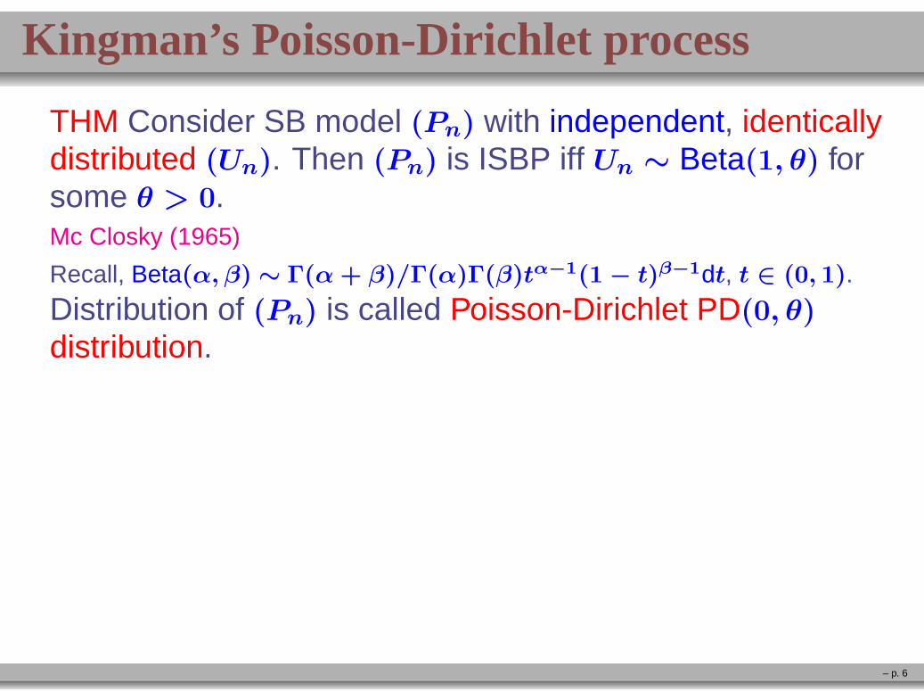
THM Consider SB model (Pn) with independent, identicallydistributed (Un). Then (Pn) is ISBP iff Un ∼ Beta(1, θ) forsome θ > 0.Mc Closky (1965)
Recall, Beta(α, β) ∼ Γ(α+ β)/Γ(α)Γ(β)tα−1(1 − t)β−1dt, t ∈ (0, 1).
Distribution of (Pn) is called Poisson-Dirichlet PD(0, θ)
distribution.
– p. 6

Kingman’s Poisson-Dirichlet process
THM Consider SB model (Pn) with independent, identicallydistributed (Un). Then (Pn) is ISBP iff Un ∼ Beta(1, θ) forsome θ > 0.Mc Closky (1965)
Recall, Beta(α, β) ∼ Γ(α+ β)/Γ(α)Γ(β)tα−1(1 − t)β−1dt, t ∈ (0, 1).
Distribution of (Pn) is called Poisson-Dirichlet PD(0, θ)
distribution.
THM Let Θθ be Poisson process on (0,∞) of intensity
θt−1e−t dt, with θ > 0. Let{
Vi :=Yi∑j Yj, Yi ∈ Θθ
}
. Then the
SBP (Vi) of {Vn} has PD(0, θ) distribution.Kingman (1975)
– p. 6
Kingman’s Poisson-Dirichlet process
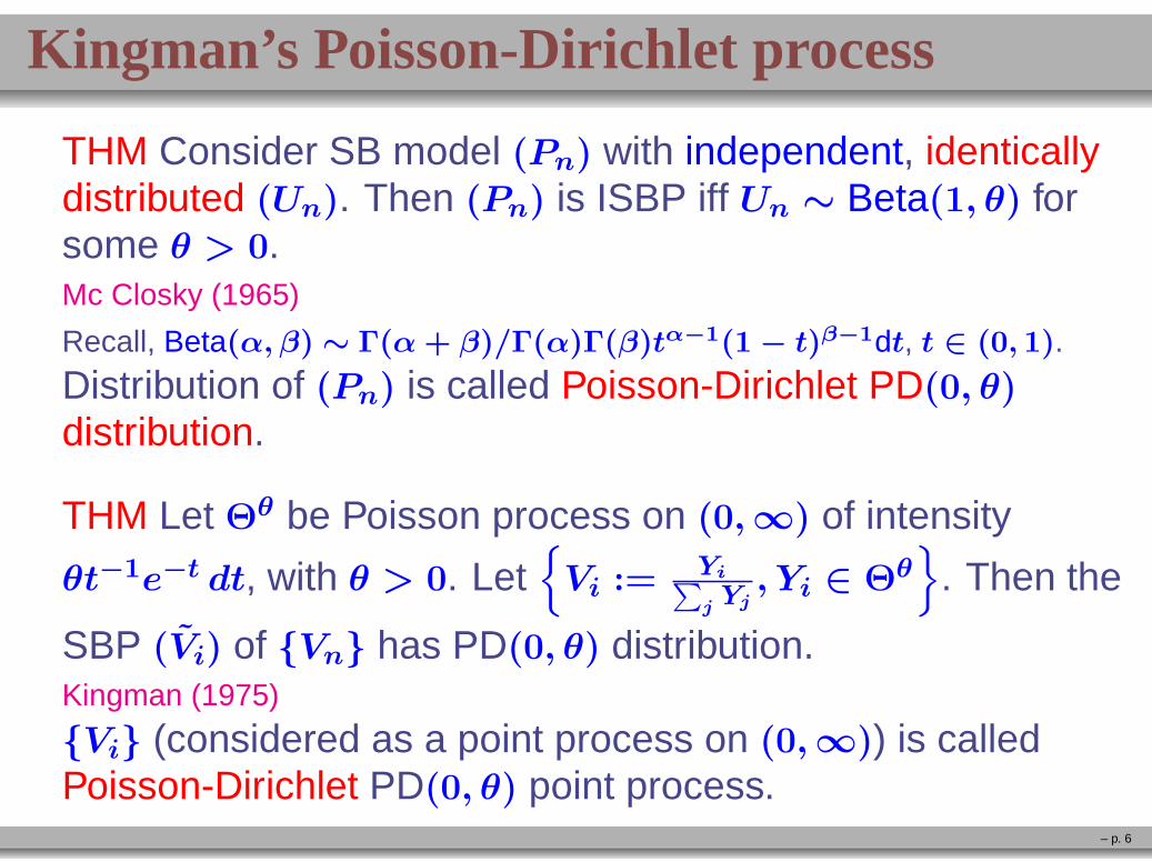
THM Consider SB model (Pn) with independent, identicallydistributed (Un). Then (Pn) is ISBP iff Un ∼ Beta(1, θ) forsome θ > 0.Mc Closky (1965)
Recall, Beta(α, β) ∼ Γ(α+ β)/Γ(α)Γ(β)tα−1(1 − t)β−1dt, t ∈ (0, 1).
Distribution of (Pn) is called Poisson-Dirichlet PD(0, θ)
distribution.
THM Let Θθ be Poisson process on (0,∞) of intensity
θt−1e−t dt, with θ > 0. Let{
Vi :=Yi∑j Yj, Yi ∈ Θθ
}
. Then the
SBP (Vi) of {Vn} has PD(0, θ) distribution.Kingman (1975)
{Vi} (considered as a point process on (0,∞)) is calledPoisson-Dirichlet PD(0, θ) point process.
– p. 6
Two-parameter Poisson-Dirichlet process
THM Consider SB model (Pn) with independent, (notnecessarily identically distributed) (Un). Then (Pn) is ISBPiff Un ∼ Beta(1 − α, θ + nα) for some α ∈ [0, 1), θ > −α.Pitman (1996)
– p. 7

Two-parameter Poisson-Dirichlet process
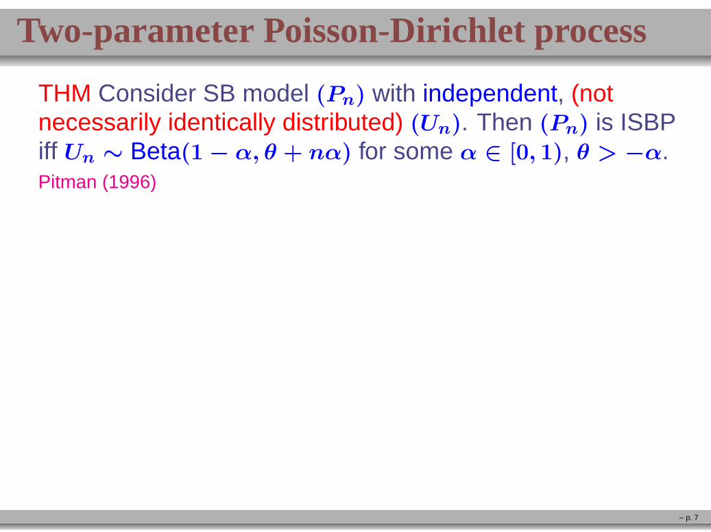
THM Consider SB model (Pn) with independent, (notnecessarily identically distributed) (Un). Then (Pn) is ISBPiff Un ∼ Beta(1 − α, θ + nα) for some α ∈ [0, 1), θ > −α.Pitman (1996)
Distribution of (Pn) is called Poisson-Dirichlet PD(α, θ)
distribution.
– p. 7
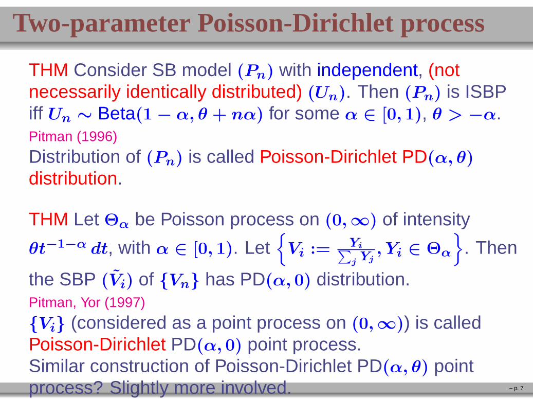
Two-parameter Poisson-Dirichlet process
THM Consider SB model (Pn) with independent, (notnecessarily identically distributed) (Un). Then (Pn) is ISBPiff Un ∼ Beta(1 − α, θ + nα) for some α ∈ [0, 1), θ > −α.Pitman (1996)
Distribution of (Pn) is called Poisson-Dirichlet PD(α, θ)
distribution.
THM Let Θα be Poisson process on (0,∞) of intensity
θt−1−α dt, with α ∈ [0, 1). Let{
Vi :=Yi∑j Yj, Yi ∈ Θα
}
. Then
the SBP (Vi) of {Vn} has PD(α, 0) distribution.Pitman, Yor (1997)
– p. 7

Two-parameter Poisson-Dirichlet process
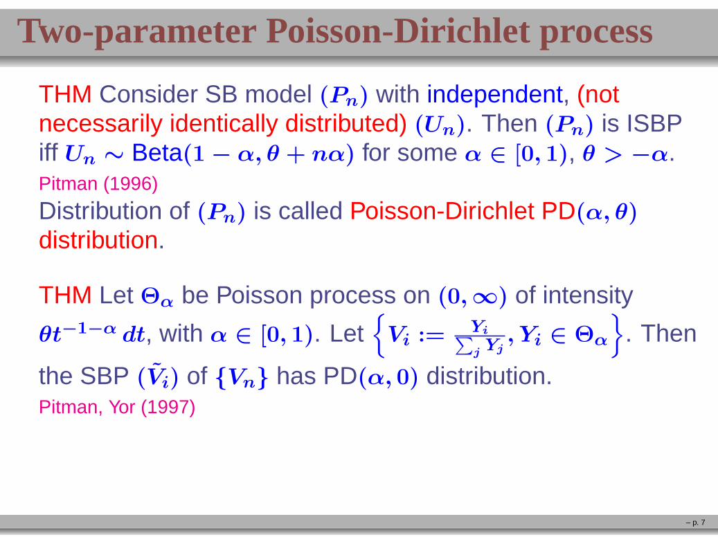
THM Consider SB model (Pn) with independent, (notnecessarily identically distributed) (Un). Then (Pn) is ISBPiff Un ∼ Beta(1 − α, θ + nα) for some α ∈ [0, 1), θ > −α.Pitman (1996)
Distribution of (Pn) is called Poisson-Dirichlet PD(α, θ)
distribution.
THM Let Θα be Poisson process on (0,∞) of intensity
θt−1−α dt, with α ∈ [0, 1). Let{
Vi :=Yi∑j Yj, Yi ∈ Θα
}
. Then
the SBP (Vi) of {Vn} has PD(α, 0) distribution.Pitman, Yor (1997)
{Vi} (considered as a point process on (0,∞)) is calledPoisson-Dirichlet PD(α, 0) point process.
– p. 7
Two-parameter Poisson-Dirichlet process
THM Consider SB model (Pn) with independent, (notnecessarily identically distributed) (Un). Then (Pn) is ISBPiff Un ∼ Beta(1 − α, θ + nα) for some α ∈ [0, 1), θ > −α.Pitman (1996)
Distribution of (Pn) is called Poisson-Dirichlet PD(α, θ)
distribution.
THM Let Θα be Poisson process on (0,∞) of intensity
θt−1−α dt, with α ∈ [0, 1). Let{
Vi :=Yi∑j Yj, Yi ∈ Θα
}
. Then
the SBP (Vi) of {Vn} has PD(α, 0) distribution.Pitman, Yor (1997)
{Vi} (considered as a point process on (0,∞)) is calledPoisson-Dirichlet PD(α, 0) point process.Similar construction of Poisson-Dirichlet PD(α, θ) pointprocess? Slightly more involved. – p. 7

PD(α, 0) vs PD(0, θ)
FACT
For PD(0, θ),∑
j Yj has Gamma(θ) distribution and is
independent of {Vi =Yi∑j Yj
}.
– p. 8

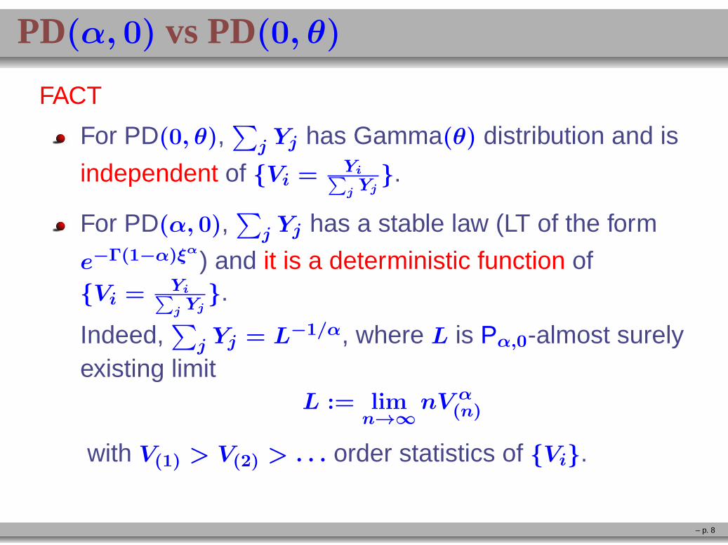
PD(α, 0) vs PD(0, θ)
FACT
For PD(0, θ),∑
j Yj has Gamma(θ) distribution and is
independent of {Vi =Yi∑j Yj
}.
For PD(α, 0),∑
j Yj has a stable law (LT of the form
e−Γ(1−α)ξα
) and it is a deterministic function of{Vi =
Yi∑j Yj
}.
– p. 8
PD(α, 0) vs PD(0, θ)
FACT
For PD(0, θ),∑
j Yj has Gamma(θ) distribution and is
independent of {Vi =Yi∑j Yj
}.
For PD(α, 0),∑
j Yj has a stable law (LT of the form
e−Γ(1−α)ξα
) and it is a deterministic function of{Vi =
Yi∑j Yj
}.
Indeed,∑
j Yj = L−1/α, where L is Pα,0-almost surelyexisting limit
L := limn→∞
nV α(n)
with V(1) > V(2) > . . . order statistics of {Vi}.
– p. 8

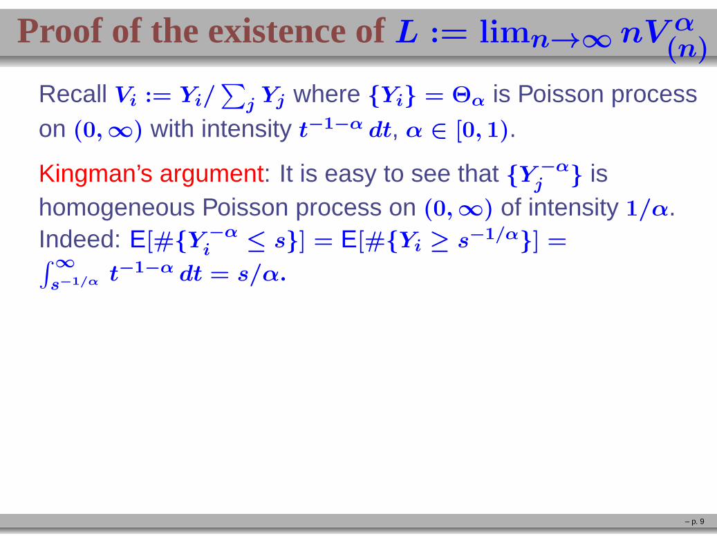
Proof of the existence ofL := limn→∞ nV α(n)
Recall Vi := Yi/∑
j Yj where {Yi} = Θα is Poisson processon (0,∞) with intensity t−1−α dt, α ∈ [0, 1).
– p. 9
Proof of the existence ofL := limn→∞ nV α(n)
Recall Vi := Yi/∑
j Yj where {Yi} = Θα is Poisson processon (0,∞) with intensity t−1−α dt, α ∈ [0, 1).
Kingman’s argument: It is easy to see that {Y −αj } is
homogeneous Poisson process on (0,∞) of intensity 1/α.Indeed: E[#{Y −α
i ≤ s}] = E[#{Yi ≥ s−1/α}] =∫∞
s−1/α t−1−α dt = s/α.
– p. 9

Proof of the existence ofL := limn→∞ nV α(n)
Recall Vi := Yi/∑
j Yj where {Yi} = Θα is Poisson processon (0,∞) with intensity t−1−α dt, α ∈ [0, 1).
Kingman’s argument: It is easy to see that {Y −αj } is
homogeneous Poisson process on (0,∞) of intensity 1/α.Indeed: E[#{Y −α
i ≤ s}] = E[#{Yi ≥ s−1/α}] =∫∞
s−1/α t−1−α dt = s/α.
Consequently, Y −α(i+1)
− Y −α(i)
are iid exponential variableswith mean α and thus by the LLN a.s.limn→∞ Y −α
(n)/n = limn 1/n
∑ni=1(Y
−α(i+1)
− Y −α(i)
) = α.
Finally,
nV α(n) = n
(
∑
j Yj
Y −α(n)
)−α
=n
Y −α(n)
(
∑
j
Yj
)−α
→(∑
j Yj)−α
α.
– p. 9

Change-of-measure representation
Pitman, Yor (1997).
Eα,θ[f({Vi})] = Cα,θEα,0[Lθ/αf({Vi})] ,
whereCα,θ = 1/Eα,0[L
θ/α] = Γ(1 − α)θ/αΓ(θ + 1)/Γ(θ/α+ 1).
– p. 10
SINR and Poisson-Dirichlet processes
– p. 11
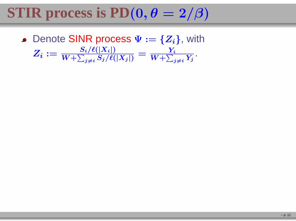
STIR process is PD(0, θ = 2/β)
Denote SINR process Ψ := {Zi}, withZi :=
Si/ℓ(|Xi|)W+
∑j 6=i Sj/ℓ(|Xj|)
= Yi
W+∑
j 6=i Yj.
– p. 12

STIR process is PD(0, θ = 2/β)
Denote SINR process Ψ := {Zi}, withZi :=
Si/ℓ(|Xi|)W+
∑j 6=i Sj/ℓ(|Xj|)
= Yi
W+∑
j 6=i Yj.
Recall Θ = {Yi} is Poisson pp of intensity2a/βt−1−2/β dt, on (0,∞), equal (modulo irrelevant inthis context constant 2a/β) to this of Θα, with α = 2/β.Recall, Θα gives rise to PD(α, 0) via similar (to SINR)points’ normalization Vi =
Yi∑j Yj
.
Recall SINR process Ψ := {Zi} can be easy related toSTINR process Ψ′ := {Z′
i :=Yi
W+∑
j Yj} via Z′
i =Zi
1+Zi.
Consequently, in case of no noise (W = 0),STIR Ψ′ is PD(0, α = 2/β).Many distributional characteristics of PD(0, α) aredeveloped in Pitman, Yor (1997)! – p. 12
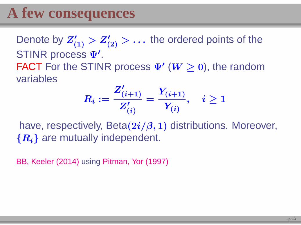
A few consequences
Denote by Z′(1) > Z′
(2) > . . . the ordered points of theSTINR process Ψ′.FACT For the STINR process Ψ′ (W ≥ 0), the randomvariables
Ri :=Z′
(i+1)
Z′(i)
=Y(i+1)
Y(i)
, i ≥ 1
have, respectively, Beta(2i/β, 1) distributions. Moreover,{Ri} are mutually independent.
BB, Keeler (2014) using Pitman, Yor (1997)
– p. 13

A few consequences, cont’d
Denote for i = 1, 2, . . .
Ai : =Z′
(1) + · · · + Z′(i)
Z′(i+1)
=Y(1) + · · · + Y(i)
Y(i+1)
. (1)
Σi : =Z′
(i+1) + Z′(i+2) + . . .
Z′i
=Y(i+1) + Y(i+2) + · · ·
Y(i)
. (2)
– p. 14

A few consequences, cont’d
Denote for i = 1, 2, . . .
Ai : =Z′
(1) + · · · + Z′(i)
Z′(i+1)
=Y(1) + · · · + Y(i)
Y(i+1)
. (1)
Σi : =Z′
(i+1) + Z′(i+2) + . . .
Z′i
=Y(i+1) + Y(i+2) + · · ·
Y(i)
. (2)
Observe that Σ−1i corresponds to SIR with
successive-interference cancellation in case W = 0.;cf. Zhang, Haenggi (2013).
– p. 14

A few consequences, cont’d
Denote for i = 1, 2, . . .
Ai : =Z′
(1) + · · · + Z′(i)
Z′(i+1)
=Y(1) + · · · + Y(i)
Y(i+1)
. (1)
Σi : =Z′
(i+1) + Z′(i+2) + . . .
Z′i
=Y(i+1) + Y(i+2) + · · ·
Y(i)
. (2)
Observe that Σ−1i corresponds to SIR with
successive-interference cancellation in case W = 0.;cf. Zhang, Haenggi (2013).Similarly,(1 +Ai−1)/Σi = (Y(1) + · · · + Y(i))/(Y(i+1) + Y(i+2) + · · · )
corresponds to SIR with signal combination in case W = 0.;cf. BB, Keeler (2015).
– p. 14

A few consequences, cont’d
For γ ≥ 0 let
φβ(γ) :=2
β
∫ ∞
1
e−γxx−2/β−1dx, (3)
ψβ(γ) := Γ(1 − 2/β)γ2/β + φβ(γ). (4)
– p. 15

A few consequences, cont’d
For γ ≥ 0 let
φβ(γ) :=2
β
∫ ∞
1
e−γxx−2/β−1dx, (3)
ψβ(γ) := Γ(1 − 2/β)γ2/β + φβ(γ). (4)
FACT Consider the STINR process Ψ′ (W ≥ 0). Then Ai−1
is distributed as the sum of i− 1 independent copies of A1,with the characteristic function E[e−γAi−1] = (φβ(γ))
i−1; Σi
is distributed as the sum of i independent copies of Σ1, withthe characteristic function E[e−γΣi] = (ψβ(γ))
−i; and Ai−1
and Σi are independent.
using Pitman, Yor (1997)
– p. 15

A few consequences, cont’d
FACT The inverse of the k th strongest STIR (W = 0) value,1/Z′
(k), has the Laplace transform
E[e−γ/Z′(k)] = e−γ(φβ(γ))
k−1(ψβ(γ))−k.
using Pitman, Yor (1997)
cf BB, Karray, Keeler (2013).
– p. 16

A few consequences, cont’d
FACT The inverse of the k th strongest STIR (W = 0) value,1/Z′
(k), has the Laplace transform
E[e−γ/Z′(k)] = e−γ(φβ(γ))
k−1(ψβ(γ))−k.
using Pitman, Yor (1997)
cf BB, Karray, Keeler (2013).
Observe, 1/Z′(k) ≤ 1/t (t ≤ 1) is equivalent to Z′
(k) ≥ t, andfurther equivalent to Z(k) ≥ t/(1 − t) (relation betweenSTINR and SINR). Consequently, the above result givesalternative approach to calculate the stationary SIR (W = 0)k-coverage probabilities pk with τ = 1/1 − t.
– p. 16

A few consequences, cont’d
FACT For the STINR process (W ≥ 0),
W/I =(
∑∞i=1 Z
′(i)
)−1
− 1, and W + I = (L/a)−β/2, with
L := limi→∞ i(Z′(i))
2/β existing almost surely.Thus, (theoretically) one can recover the values of thereceived powers and the noise from the SINRmeasurements.
using Pitman, Yor (1997)
– p. 17

“Introducing W > 0 to Poisson-Dirichlet”from STIR to STINR
– p. 18
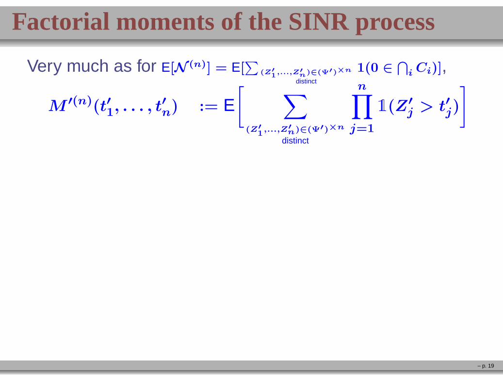
Factorial moments of the SINR process
Very much as for E[N (n)] = E[∑
(Z′1,...,Z′
n)∈(Ψ′)×n
distinct
1(0 ∈⋂
iCi)],
M ′(n)(t′1, . . . , t′n) := E
[
∑
(Z′1,...,Z′
n)∈(Ψ′)×n
distinct
n∏
j=1
1(Z′j > t′j)
]
– p. 19
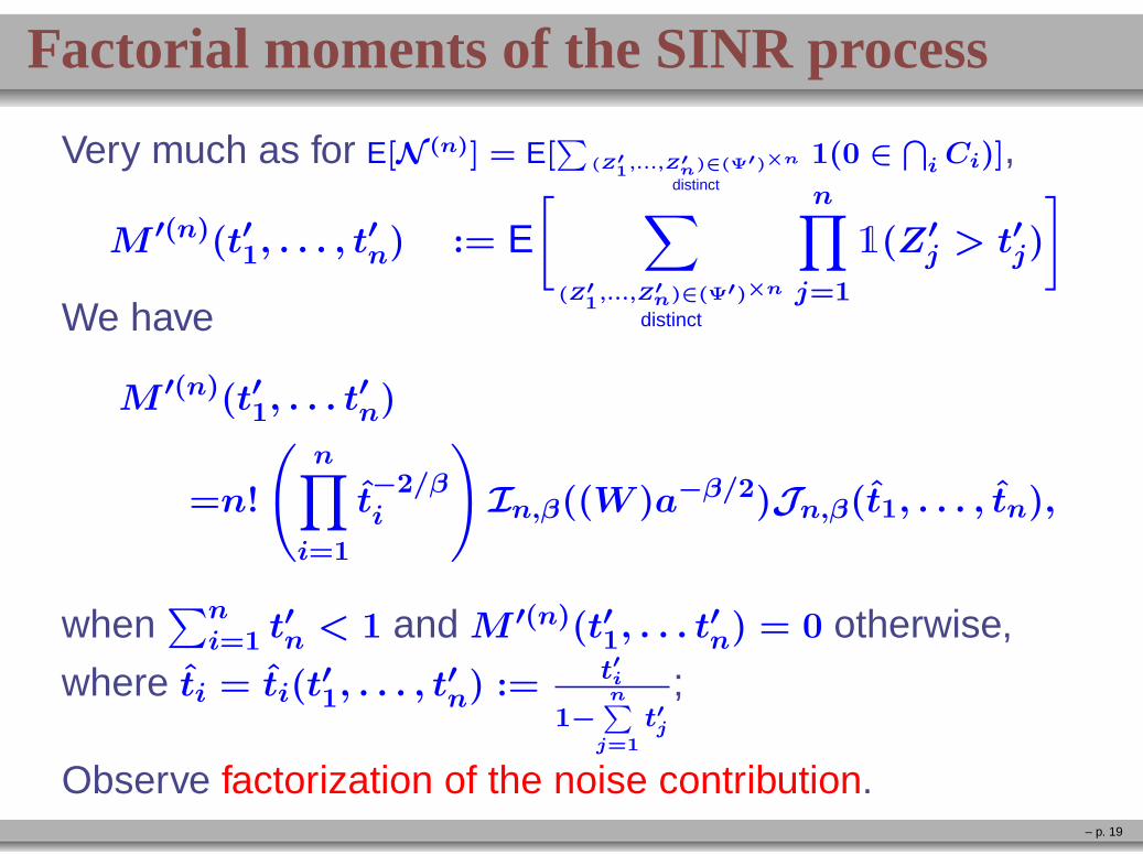
Factorial moments of the SINR process
Very much as for E[N (n)] = E[∑
(Z′1,...,Z′
n)∈(Ψ′)×n
distinct
1(0 ∈⋂
iCi)],
M ′(n)(t′1, . . . , t′n) := E
[
∑
(Z′1,...,Z′
n)∈(Ψ′)×n
distinct
n∏
j=1
1(Z′j > t′j)
]
We have
M ′(n)(t′1, . . . t′n)
=n!
(
n∏
i=1
t−2/βi
)
In,β((W )a−β/2)Jn,β(t1, . . . , tn),
when∑n
i=1 t′n < 1 and M ′(n)(t′1, . . . t
′n) = 0 otherwise,
where ti = ti(t′1, . . . , t
′n) := t′i
1−n∑
j=1
t′j
;
Observe factorization of the noise contribution.– p. 19

Factorial moments of PD processes
Very simple thanks to SB (stick-braking) representation!
– p. 20

Factorial moments of PD processes
Very simple thanks to SB (stick-braking) representation!
Indeed, for the fist moment measure MPD(dt),
∫ 1
0
f(t)MPD(dt) := E[
∑
i
f(Vi)]
= E[
∑
i
f(Vi)
ViVi
]
= E[f(V1)
V1
]
where {Vi} SBP of {Vi}
– p. 20

Factorial moments of PD processes
Very simple thanks to SB (stick-braking) representation!
Indeed, for the fist moment measure MPD(dt),
∫ 1
0
f(t)MPD(dt) := E[
∑
i
f(Vi)]
= E[
∑
i
f(Vi)
ViVi
]
= E[f(V1)
V1
]
where {Vi} SBP of {Vi}
hence MPD(dt) = 1/t× FVi(dt) and and we know that
Vi = U1 ∼ Beta(1 − α, θ + 1 × α).
– p. 20

Factorial moments of PD processes, cont’d
Similarly, by the induction, using ISBP representation of PD,the density µ(n)
PD (t1, . . . , tn) of the n th factorial momentmeasure of the PD(α, 0) process can be easily shown to be
µ(n)PD (t1, . . . , tn) = cn,2/β,0
(
n∏
i=1
(t′i)−(2/β+1)
)(
1−n∑
j=1
(t′j))2n/β−1
,
where
cn,α,θ =
n∏
i=1
Γ(θ + 1 + (i− 1)α)
Γ(1 − α)Γ(θ + iα);
(related to the Beta distributions of independent {Un} in SBmodel of PD).Handa (2009).
– p. 21
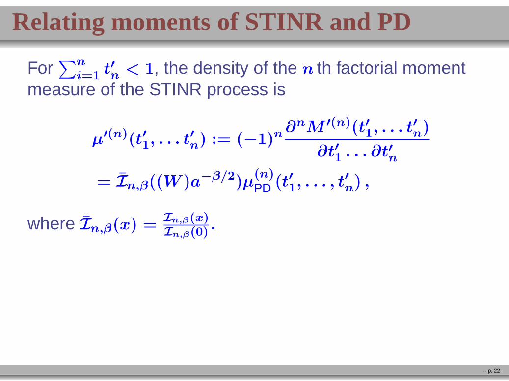
Relating moments of STINR and PD
For∑n
i=1 t′n < 1, the density of the n th factorial moment
measure of the STINR process is
µ′(n)(t′1, . . . t′n) := (−1)n
∂nM ′(n)(t′1, . . . t′n)
∂t′1 . . . ∂t′n
= In,β((W )a−β/2)µ(n)PD (t′1, . . . , t
′n) ,
where In,β(x) =In,β(x)In,β(0)
.
– p. 22

General factorial moment expansions
Expansions of general characteristics φ of the STINRprocess
E[φ(Ψ′)] = φ(∅) +∞∑
n=1
∫
(0,1)nφt′1,...,t
′nµ′(n)(t′1, . . . , t
′n) dt
′n . . . dt
′1 ,
where
φt′1 = φ({t′1}) − φ(∅)
φt′1,t′2=
1
2
(
φ({t′1, t′2}) − φ({t′1}) − φ({t′2}) + φ(∅)
)
. . .
φt′1,...,t′n=
1
n!
n∑
k=0
(−1)n−k∑
t′i1
,...,t′ik
distinct
φ({t′i1, . . . , t′ik}) .
BB (1995).– p. 23

Numerical examples
– p. 24

k-coverage probabilities
−10 −8 −6 −4 −2 0 2 40
0.2
0.4
0.6
0.8
1
τ(dB)
P(k) (τ)
k=1
k=2
k=3
β = 3
−10 −8 −6 −4 −2 0 2 40
0.2
0.4
0.6
0.8
1
τ(dB)P
(k) (τ)
k=1
k=2
k=3
β = 5
SINR k-coverage probability
– p. 25
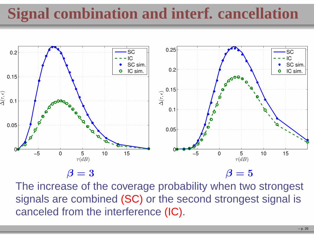
Signal combination and interf. cancellation
−5 0 5 10 150
0.05
0.1
0.15
0.2
τ(dB)
∆(τ,ǫ)
SC
IC
SC sim.
IC sim.
β = 3
−5 0 5 10 150
0.05
0.1
0.15
0.2
0.25
τ(dB)∆(τ,ǫ)
SC
IC
SC sim.
IC sim.
β = 5
The increase of the coverage probability when two strongestsignals are combined (SC) or the second strongest signal iscanceled from the interference (IC).
– p. 26

Conclusions
We have seen a Poisson-Dirichlet process in somewireless communication model, where it describes“fractions” of the SINR spectrum. But Poisson-Dirichletprocesses appear in several apparently differentcontexts.
– p. 27

Conclusions
We have seen a Poisson-Dirichlet process in somewireless communication model, where it describes“fractions” of the SINR spectrum. But Poisson-Dirichletprocesses appear in several apparently differentcontexts.
“Two-parameter” family of Poisson-Dirichlet processesappear naturally in genetic population models inequilibrium ans well as in math/economic models (whereit represents e.g. factions of the market owned bydifferent companies).
– p. 27

Conclusions, cont’d
In math/physics “our” PD(α, 0) process appears as thethermodynamic (large system) limit in the lowtemperature regime of Derrida’s random energy model(REM). It is also a key component of the so-called Ruelleprobability cascades, which are used to represent thethermodynamic limit of the Sherrington-Kirkpatrickmodel for spin glasses (types of disordered magnets).
– p. 28

Relations to the PD processes give some universality to theSINR model, initially motivated by wireless communications.This may hopefully attract some further interest to thismodel.
thank you
– p. 29