Oil & Natural Gas Technology - National Energy … Library/Research/Oil-Gas/methane... · Oil &...

Oil & Natural Gas Technology

DOE Award No.: DE-FC26-06NT42962

Material Balance Study (Topical Report)

Characterization and Quantification of the

Methane Hydrate Resource Potential Associated with the Barrow Gas Fields

Submitted by: Petrotechnical Resources of Alaska, LLC

3601 C. Street, Suite 822 Anchorage, AK 99503

Prepared for:

United States Department of Energy National Energy Technology Laboratory

March, 2008

Office of Fossil Energy

Topical Report:

Material Balance Study to Investigate Methane Hydrate Resource Potential

in the East Pool of the Barrow Gas Field

March 2008

CHARACTERIZATION AND QUANTIFICATION

OF THE METHANE HYDRATE RESOURCE POTENTIAL ASSOCIATED WITH THE

BARROW GAS FIELDS

DOE Project Number: DE-FC26-06NT42962

Awarded to

North Slope Borough, Alaska

Project Director/Manager: Kent Grinage

Principal Investigator: Thomas P. Walsh

Prepared by

Praveen Singh

University of Alaska – Fairbanks

College of Engineering & Mines

PO Box 755880

Fairbanks AK 99775-5880

and

Manmath Panda and Peter J. Stokes

Petrotechnical Resources of Alaska, LLC

3601 C. Street, Suite 822

Anchorage, AK 99503

Prepared for:

U.S. Department of Energy

National Energy Technology Laboratory

626 Cochrane Mills Road

P.O. Box 10940

Pittsburgh, PA 15236-0940

DE-FC26-06NT42962 Topical Report on Material Balance - March 2008 ii

DISCLAIMER

This report was prepared as an account of work sponsored by an agency of the United States

Government. Neither the Untied States Government nor any agency thereof, nor any of their employees,

makes any warranty, express or implied, or assumes any legal liability or responsibility for the accuracy,

completeness, or usefulness of any information, apparatus, product, or process disclosed, or represents

that its use would not infringe privately owned rights. Reference herein to any specific commercial

product, process, or service by trade name, trademark, manufacturer, or otherwise does not necessarily

constitute or imply its endorsement, recommendation, or favoring by the Untied States Government or

any agency thereof. The views and opinions of authors expressed herein do not necessarily state or

reflect those of the United States Government or any agency thereof.

DE-FC26-06NT42962 Topical Report on Material Balance - March 2008 iii

TABLE OF CONTENTS

Section Page

Table of Contents iii

List of Figures iv

Executive Summary 1

Summary of Project 1

Topical Report Introduction 4

Approach to Material Balance Analysis of East Pool, Barrow Gas Field 4

Volumetric Reservoir Analysis 4

Water Influx Analysis 6

Methane Hydrate Material Balance Analysis 7

Topical Report Conclusion 11

References 13

Appendix A: Reservoir Description of East Pool, Barrow Gas Field 14

Appendix B: Extended Material Balance Technique by West & Cochrane, 1994 19

Appendix C: Water Influx Model by Pletcher, 2002 and Ahmed & McKinney, 2005 22

Appendix D: Hydrate Material Balance Model by Gerami & Darvish, 2006 24

DE-FC26-06NT42962 Topical Report on Material Balance - March 2008 iv

LIST OF FIGURES

Figure Page

Figure 1. Map of Barrow Gas Fields in North Slope Borough of Alaska 1

Figure 2: EMB Model – P/Z vs. Gp plot for East Barrow gas reservoir 5

Figure 3: EMB Model – Pressure (P) vs. Time plot for East Barrow gas reservoir 6

Figure 4: Water in Influx Model - (GpBg + WpBw) / (Bg − Bgi) vs. Gp plot 7

Figure 5: Hydrate Model: P/Z comparison for Volumetric and Modified Darvish Model 8

Figure 6: Hydrate Model: Pressure profile for Volumetric & Darvish Model 8

Figure 7: Hydrate Model: P/Z vs. Gp for East Barrow type reservoir without hydrates 9

Figure 8: Hydrate Model: Pressure vs. Time for East Barrow type reservoir without hydrates 9

Figure 9: Hydrate Model: P/Z vs. Gp comparison for Darvish model 10

Figure 10: Hydrate Model : Pressure vs. Time comparison for Darvish model 11

DE-FC26-06NT42962 Topical Report on Material Balance - March 2008 Page 1 of 26

EXECUTIVE SUMMARY

This Topical Report details the material balance modeling that was performed to explain the production

history performance results for the East Barrow Field with either volumetric gas expansion, volumetric

gas expansion coupled with aquifer support, or hydrate dissociation, gas expansion and aquifer support.

This material balance modeling was done to ensure that the further reservoir simulation with a full field

model to describe the hydrate reservoir system was justified in Phase IB of this project.

The material balance modeling results indicated that volumetric expansion and aquifer support combined

could not explain the pressure response of the reservoir, and that hydrate dissociation must be a factor.

The material balance study confirmed the existence of a thick hydrate layer overlying the free gas zone

within East Barrow reservoir. The analysis also shows an association of a weak aquifer providing partial

pressure support to the gas reservoir. Results obtained for the hydrate-capped free gas reservoir with weak

aquifer support closely matched the production data with a maximum percentage error of 10%.

SUMMARY OF PROJECT

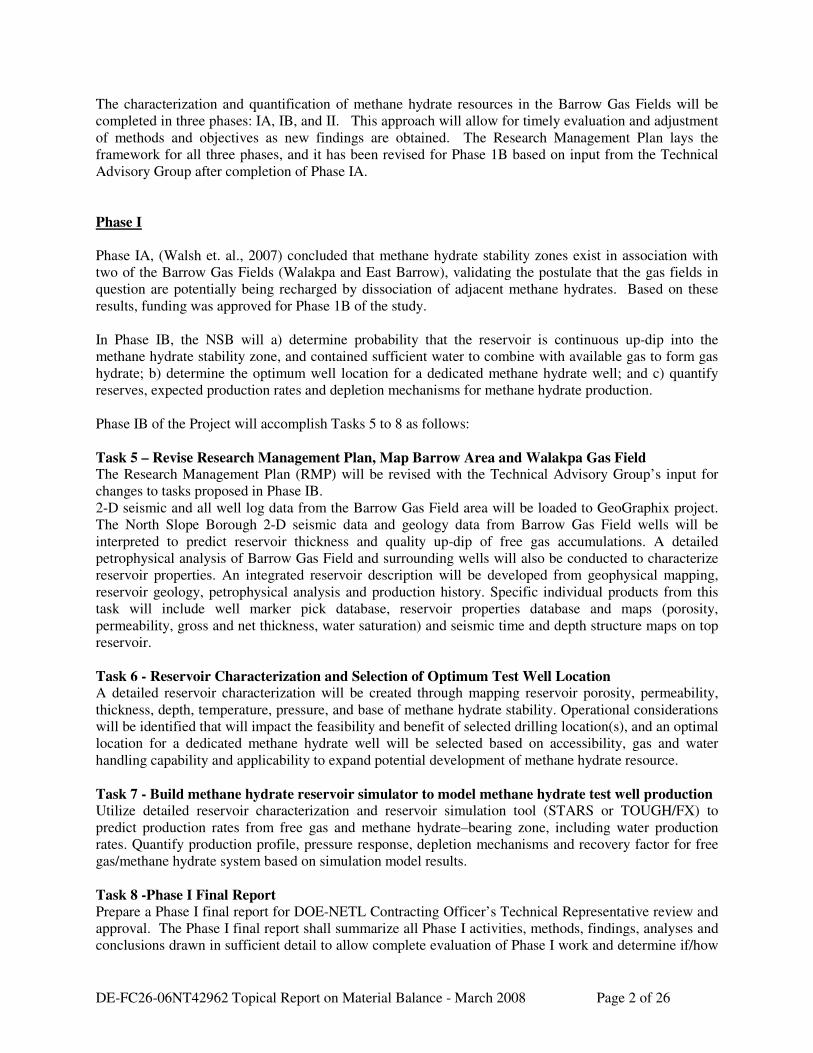
The North Slope Borough (NSB) has established a team to characterize and quantify the methane hydrate

resource potential associated with the Barrow Gas Fields, which are owned and operated by the NSB in a

permafrost region of arctic Alaska. Currently, gas from these three producing fields provides heating and

electricity for Barrow, which is the economic, transportation, and administrative center of the NSB.

Other commercially-operated producing oil and gas fields within the NSB include Prudhoe Bay, Milne

Point, Kuparuk, Alpine and Endicott. The results of this project will enhance the understanding of the

nature and occurrence of methane hydrates in the arctic environment, and specifically in the Barrow Gas

Fields, and will serve to evaluate the potential influence of gas hydrates on gas supply and production

from producing gas fields. Findings of this project will contribute significantly to understanding the role

of gas hydrate as a recharge mechanism in a producing gas field, and provide substantial commercial and

social benefits for the NSB. Figure 1 shows a map of the Barrow Area.

Figure 1: Map of Barrow Gas Fields in North Slope Borough of Alaska


The characterization and quantification of methane hydrate resources in the Barrow Gas Fields will be

completed in three phases: IA, IB, and II. This approach will allow for timely evaluation and adjustment

of methods and objectives as new findings are obtained. The Research Management Plan lays the

framework for all three phases, and it has been revised for Phase 1B based on input from the Technical

Advisory Group after completion of Phase IA.

Phase I

Phase IA, (Walsh et. al., 2007) concluded that methane hydrate stability zones exist in association with

two of the Barrow Gas Fields (Walakpa and East Barrow), validating the postulate that the gas fields in

question are potentially being recharged by dissociation of adjacent methane hydrates. Based on these

results, funding was approved for Phase 1B of the study.

In Phase IB, the NSB will a) determine probability that the reservoir is continuous up-dip into the

methane hydrate stability zone, and contained sufficient water to combine with available gas to form gas

hydrate; b) determine the optimum well location for a dedicated methane hydrate well; and c) quantify

reserves, expected production rates and depletion mechanisms for methane hydrate production.

Phase IB of the Project will accomplish Tasks 5 to 8 as follows:

Task 5 – Revise Research Management Plan, Map Barrow Area and Walakpa Gas Field The Research Management Plan (RMP) will be revised with the Technical Advisory Group’s input for

changes to tasks proposed in Phase IB.

2-D seismic and all well log data from the Barrow Gas Field area will be loaded to GeoGraphix project.

The North Slope Borough 2-D seismic data and geology data from Barrow Gas Field wells will be

interpreted to predict reservoir thickness and quality up-dip of free gas accumulations. A detailed

petrophysical analysis of Barrow Gas Field and surrounding wells will also be conducted to characterize

reservoir properties. An integrated reservoir description will be developed from geophysical mapping,

reservoir geology, petrophysical analysis and production history. Specific individual products from this

task will include well marker pick database, reservoir properties database and maps (porosity,

permeability, gross and net thickness, water saturation) and seismic time and depth structure maps on top

reservoir.

Task 6 - Reservoir Characterization and Selection of Optimum Test Well Location A detailed reservoir characterization will be created through mapping reservoir porosity, permeability,

thickness, depth, temperature, pressure, and base of methane hydrate stability. Operational considerations

will be identified that will impact the feasibility and benefit of selected drilling location(s), and an optimal

location for a dedicated methane hydrate well will be selected based on accessibility, gas and water

handling capability and applicability to expand potential development of methane hydrate resource.

Task 7 - Build methane hydrate reservoir simulator to model methane hydrate test well production Utilize detailed reservoir characterization and reservoir simulation tool (STARS or TOUGH/FX) to

predict production rates from free gas and methane hydrate–bearing zone, including water production

rates. Quantify production profile, pressure response, depletion mechanisms and recovery factor for free

gas/methane hydrate system based on simulation model results.

Task 8 -Phase I Final Report Prepare a Phase I final report for DOE-NETL Contracting Officer’s Technical Representative review and

approval. The Phase I final report shall summarize all Phase I activities, methods, findings, analyses and

conclusions drawn in sufficient detail to allow complete evaluation of Phase I work and determine if/how


to proceed with Phase II. If the decision is made not to continue to Phase II, the Phase I Final Report will

be resubmitted as the Final Scientific/Technical Report, in accordance with Attachment F, Federal

Assistance Reporting Checklist and instructions.

The results of Phase IB will determine whether or not funding will be requested for Phase II.

Transition to Phase II

If the decision is made to proceed with Phase II, the RMP will be updated and revised, with an expanded

Statement of Project Objectives (SOPO ) and definitive estimate to be approved by the DOE COR before

proceeding with Phase II work. The following information regarding Phase II tasks and objectives is

provided for strategic planning purposes, and is preliminary in nature. Estimated costs and resources

will be provided in detail if and when a decision to proceed to Phase II is reached.

Phase II

The goal of Phase II is to drill and test a dedicated methane hydrate well near Barrow. Phase II will be the

subject of future funding decisions contingent on the results of Phase I, as described above. If a decision

is made to proceed with Phase II, the scope of work will be refined during or at the end of Phase I.

Currently, the work objectives for Phase II are to:

• Design a dedicated methane hydrate well to be drilled up-dip of one of the three Barrow Gas

Fields,

• Drill and complete the well,

• Design and implement a surveillance program to analyze production from the methane hydrate

well

To satisfy these objectives, the tasks currently proposed are summarized below.

Task 9—Design and drill a well at or near the methane hydrate/free gas interface This work will take into account the associated operational complexities, commercial viability, and data

gathering needs. Consider high angle or horizontal well to improve probability of intersecting interface

and to help avoid produced water handling issues at the surface.

Task 10—Measure changes in the free gas interval Measure changes including pressure, temperature, gas composition, production rate and the methane

hydrate zone (pressure, temperature, depth of interface) to understand the depletion mechanisms and

interactions between free gas zone and methane hydrate zone.

Task 11 —Final Report Provide final report, as identified in the Federal Assistance Reporting Checklist. The report will

thoroughly detail all activities conducted under Phase I and 2 of the project. Provide detailed description

of all work undertaken, methods used to conduct work, data and information resulting from this work,

descriptive analysis of results and conclusions. Information contained in the report will cover all tasks

conducted and will include (report or appendices) all supporting documentation (e.g., software code,

drawings, maps, etc.). The final report will provide a listing of all professional publications, technical

papers and/or presentations generated as a result of project activities.


TOPICAL REPORT INTRODUCTION

Gruy, 1978 originally mapped the East Pool of the Barrow Field and determined from log analysis and

production testing that a gas oil contact was encountered in well S Barrow 17 at -2081’ SS.

Allen and Crouch, 1988 described the material balance performance of the East Barrow Pool as showing

strong aquifer support. They predicted OGIP of 6.2 BCF and that the reservoir would soon be watering

out.

Phase IA studies by Walsh, et. al., 2007 demonstrated a strong probability that portions of the East

Barrow Pool and sands up dip are in the methane hydrate stability zone. The combination of

repressurization of the reservoir and the extent of the hydrate stability zone are evidence that there is a

strong presence of insitu hydrates.

The hydrate stability model was based on temperature gradient, pressure gradient and gas analysis data. It

was assumed that the reservoir has sufficient water and gas required for hydrate formation. With an aim to

substantiate the fact that the reservoir has associated hydrates and in order to construct a detailed reservoir

model for production modeling work, material balance studies have been undertaken. The material

balance analysis can provide an insight into the reservoir drive mechanisms and help in estimating initial

free gas in place, strength, size of associated aquifer (if any), hydrate cap thickness (if any) etc. The

material balance analysis shall be able to strengthen the conclusions of the previous work and to provide a

platform from where one can develop a full scale reservoir model and simulate production modeling

scenarios.

APPROACH TO MATERIAL BALANCE ANALYSIS OF EAST POOL, BARROW GAS FIELD

Reservoir performance history matching using material balance models was done progressively as

follows:

• a volumetric reservoir with an iterative technique that was developed for tight shallow gas

reservoirs by West and Cochrane, 1994 called Extended Material Balance.

• a volumetric reservoir with aquifer support with an analysis technique developed by Pletcher,

2002 and Ahmed & McKinney, 2005.

• a volumetric reservoir with methane hydrate dissociation model used was developed by Gerami

& Darvish, 2006.

Appendix A details the reservoir properties and description of the E Barrow Pool.

VOLUMETRIC RESERVOIR ANALYSIS

Appendix B gives the detailed description of the Extended Material Balance (EMB) technique by West

and Cochrane, 1994.

The EMB methodology was applied to East Barrow gas reservoir. Several iterations were carried out to

obtain a constant deliverability coefficient (C). Z-factor and gas viscosity calculations were also

undertaken to provide accurate gas property. The best case (constant C) was obtained by assuming an

initial gas in place, G of 90 std bcf. The initial reserve obtained using this model is exceptionally high

compared to volumetric estimates of 15 std bcf (Gruy 1978).


The primary reason for higher EMB estimates is that the EMB method assumes a tight gas reservoir and

the iterations are aimed at providing a fixed value of deliverability constant which is possible only when

the average pressure within the reservoir remains close to initial pressure. This is physically possible only

when we have exceptionally high volumes of initial gas in place.

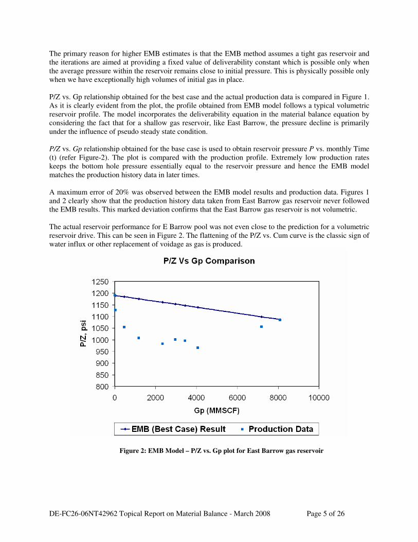
P/Z vs. Gp relationship obtained for the best case and the actual production data is compared in Figure 1.

As it is clearly evident from the plot, the profile obtained from EMB model follows a typical volumetric

reservoir profile. The model incorporates the deliverability equation in the material balance equation by

considering the fact that for a shallow gas reservoir, like East Barrow, the pressure decline is primarily

under the influence of pseudo steady state condition.

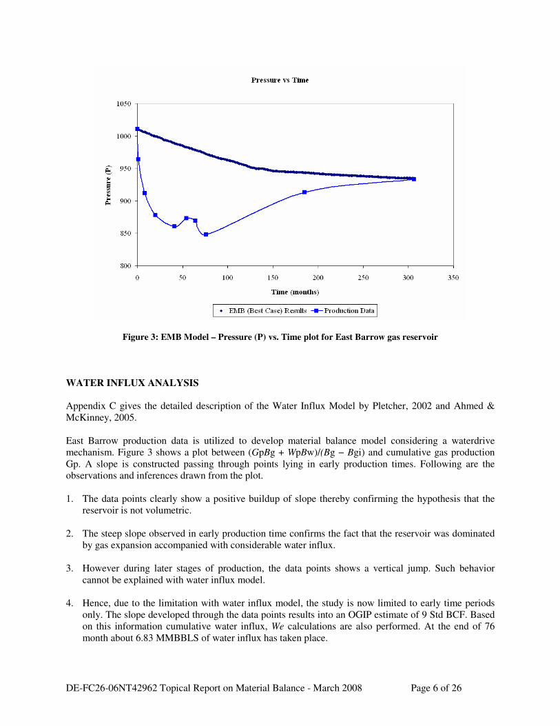
P/Z vs. Gp relationship obtained for the base case is used to obtain reservoir pressure P vs. monthly Time

(t) (refer Figure-2). The plot is compared with the production profile. Extremely low production rates

keeps the bottom hole pressure essentially equal to the reservoir pressure and hence the EMB model

matches the production history data in later times.

A maximum error of 20% was observed between the EMB model results and production data. Figures 1

and 2 clearly show that the production history data taken from East Barrow gas reservoir never followed

the EMB results. This marked deviation confirms that the East Barrow gas reservoir is not volumetric.

The actual reservoir performance for E Barrow pool was not even close to the prediction for a volumetric

reservoir drive. This can be seen in Figure 2. The flattening of the P/Z vs. Cum curve is the classic sign of

water influx or other replacement of voidage as gas is produced.

Figure 2: EMB Model – P/Z vs. Gp plot for East Barrow gas reservoir


Figure 3: EMB Model – Pressure (P) vs. Time plot for East Barrow gas reservoir

WATER INFLUX ANALYSIS

Appendix C gives the detailed description of the Water Influx Model by Pletcher, 2002 and Ahmed &

McKinney, 2005.

East Barrow production data is utilized to develop material balance model considering a waterdrive

mechanism. Figure 3 shows a plot between (GpBg + WpBw)/(Bg − Bgi) and cumulative gas production

Gp. A slope is constructed passing through points lying in early production times. Following are the

observations and inferences drawn from the plot.

1. The data points clearly show a positive buildup of slope thereby confirming the hypothesis that the

reservoir is not volumetric.

2. The steep slope observed in early production time confirms the fact that the reservoir was dominated

by gas expansion accompanied with considerable water influx.

3. However during later stages of production, the data points shows a vertical jump. Such behavior

cannot be explained with water influx model.

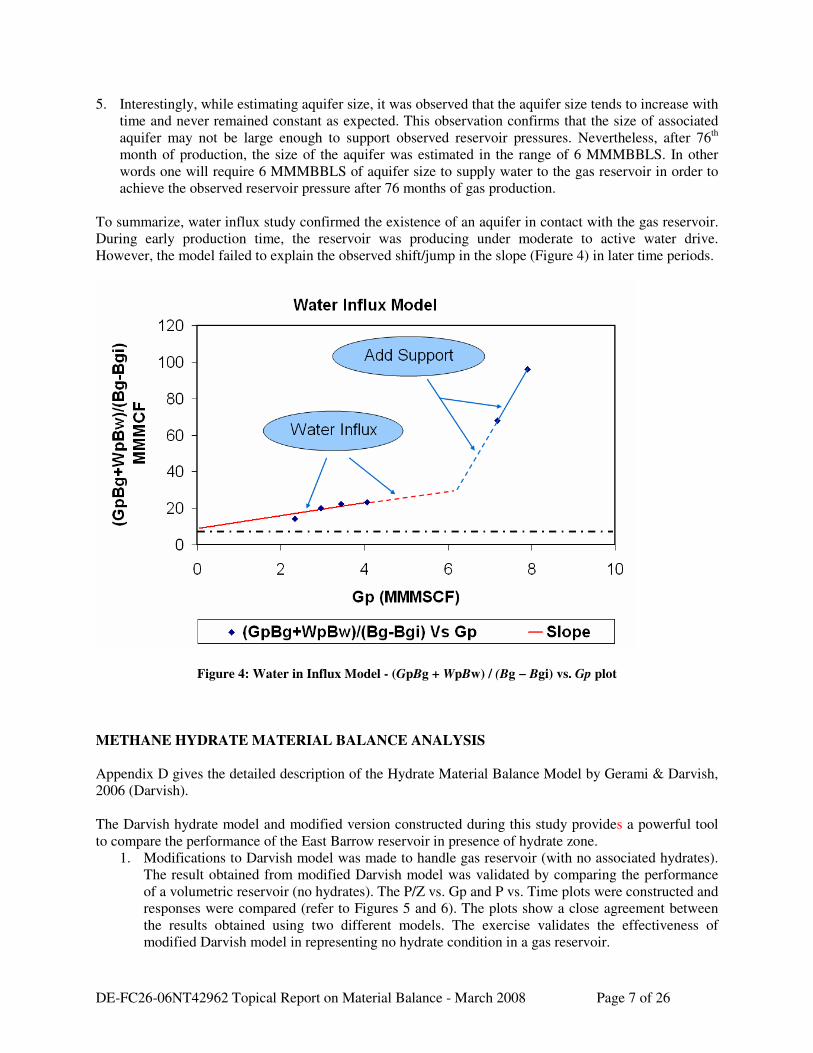
4. Hence, due to the limitation with water influx model, the study is now limited to early time periods

only. The slope developed through the data points results into an OGIP estimate of 9 Std BCF. Based

on this information cumulative water influx, We calculations are also performed. At the end of 76

month about 6.83 MMBBLS of water influx has taken place.


5. Interestingly, while estimating aquifer size, it was observed that the aquifer size tends to increase with

time and never remained constant as expected. This observation confirms that the size of associated

aquifer may not be large enough to support observed reservoir pressures. Nevertheless, after 76th

month of production, the size of the aquifer was estimated in the range of 6 MMMBBLS. In other

words one will require 6 MMMBBLS of aquifer size to supply water to the gas reservoir in order to

achieve the observed reservoir pressure after 76 months of gas production.

To summarize, water influx study confirmed the existence of an aquifer in contact with the gas reservoir.

During early production time, the reservoir was producing under moderate to active water drive.

However, the model failed to explain the observed shift/jump in the slope (Figure 4) in later time periods.

Figure 4: Water in Influx Model - (GpBg + WpBw) / (Bg − Bgi) vs. Gp plot

METHANE HYDRATE MATERIAL BALANCE ANALYSIS

Appendix D gives the detailed description of the Hydrate Material Balance Model by Gerami & Darvish,

2006 (Darvish).

The Darvish hydrate model and modified version constructed during this study provides a powerful tool

to compare the performance of the East Barrow reservoir in presence of hydrate zone.

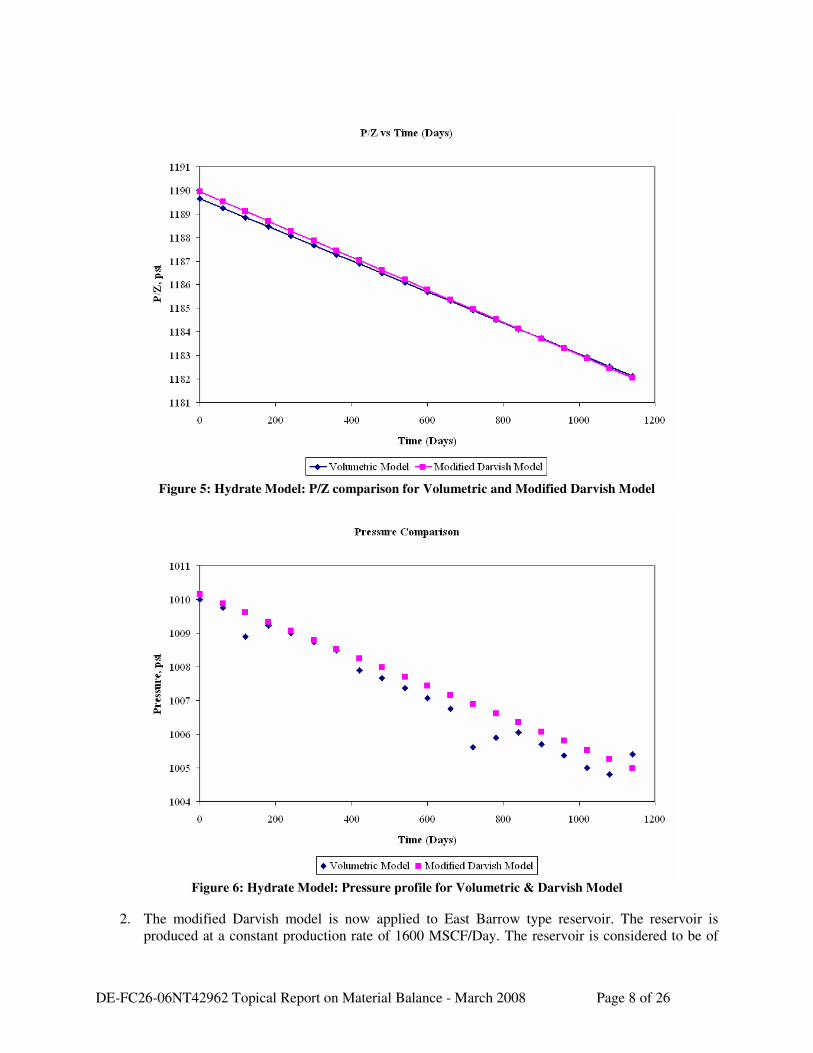
1. Modifications to Darvish model was made to handle gas reservoir (with no associated hydrates).

The result obtained from modified Darvish model was validated by comparing the performance

of a volumetric reservoir (no hydrates). The P/Z vs. Gp and P vs. Time plots were constructed and

responses were compared (refer to Figures 5 and 6). The plots show a close agreement between

the results obtained using two different models. The exercise validates the effectiveness of

modified Darvish model in representing no hydrate condition in a gas reservoir.


Figure 5: Hydrate Model: P/Z comparison for Volumetric and Modified Darvish Model

Figure 6: Hydrate Model: Pressure profile for Volumetric & Darvish Model

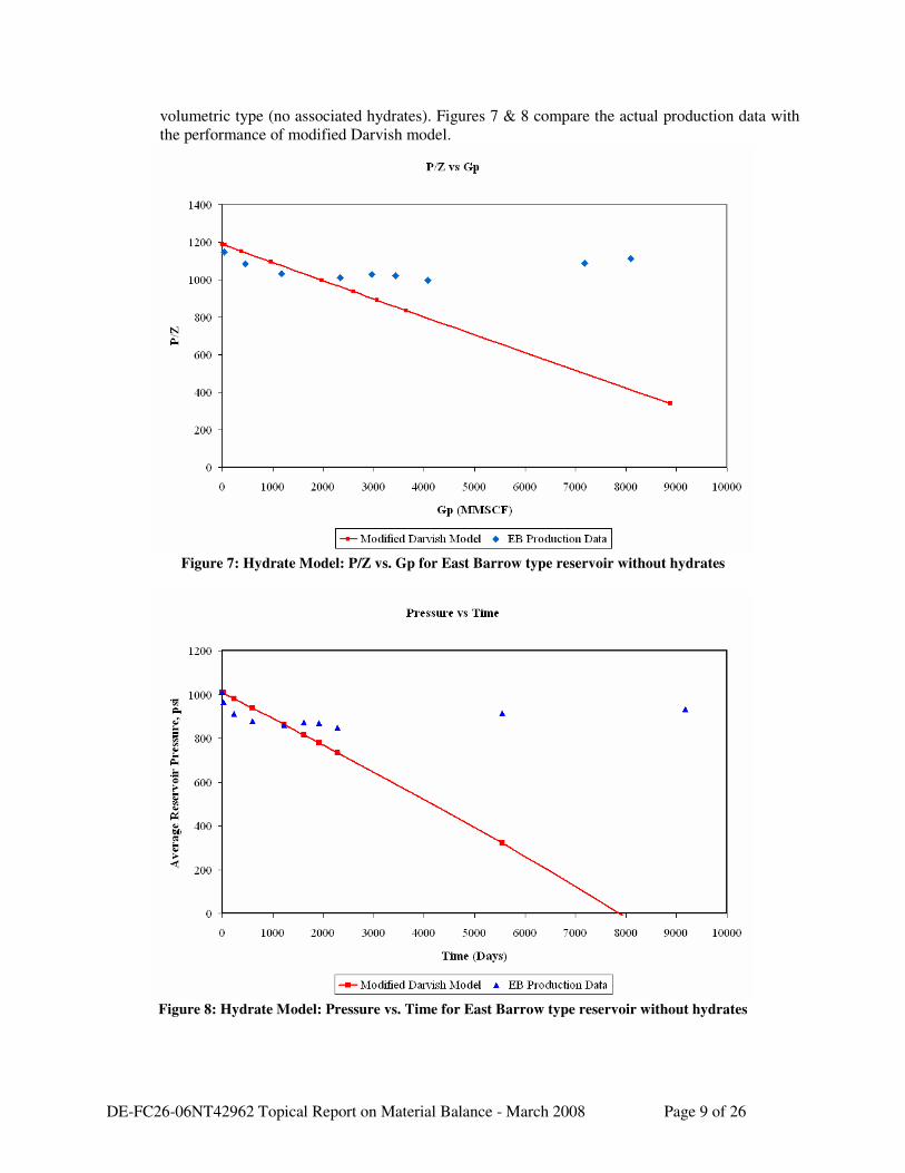
2. The modified Darvish model is now applied to East Barrow type reservoir. The reservoir is

produced at a constant production rate of 1600 MSCF/Day. The reservoir is considered to be of


volumetric type (no associated hydrates). Figures 7 & 8 compare the actual production data with

the performance of modified Darvish model.

Figure 7: Hydrate Model: P/Z vs. Gp for East Barrow type reservoir without hydrates

Figure 8: Hydrate Model: Pressure vs. Time for East Barrow type reservoir without hydrates


As expected the production data and modified Darvish results never matched during the entire

production life of the reservoir. Thus, we conclude that the reservoir is under constant pressure

support from either water influx and/or associated hydrates.

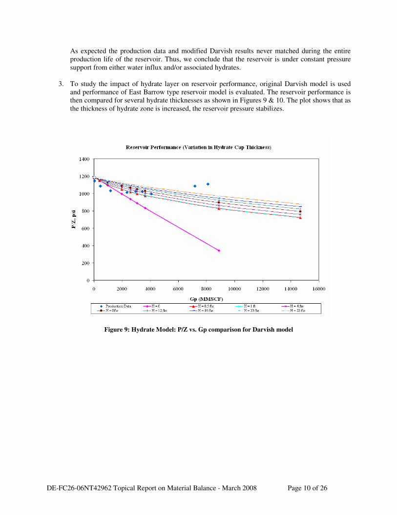
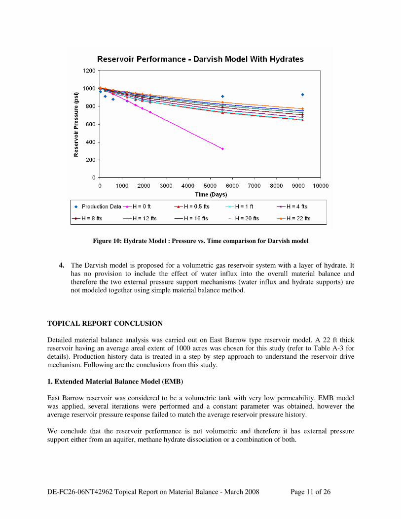
3. To study the impact of hydrate layer on reservoir performance, original Darvish model is used

and performance of East Barrow type reservoir model is evaluated. The reservoir performance is

then compared for several hydrate thicknesses as shown in Figures 9 & 10. The plot shows that as

the thickness of hydrate zone is increased, the reservoir pressure stabilizes.

Figure 9: Hydrate Model: P/Z vs. Gp comparison for Darvish model


Figure 10: Hydrate Model : Pressure vs. Time comparison for Darvish model

4. The Darvish model is proposed for a volumetric gas reservoir system with a layer of hydrate. It

has no provision to include the effect of water influx into the overall material balance and

therefore the two external pressure support mechanisms (water influx and hydrate supports) are

not modeled together using simple material balance method.

TOPICAL REPORT CONCLUSION

Detailed material balance analysis was carried out on East Barrow type reservoir model. A 22 ft thick

reservoir having an average areal extent of 1000 acres was chosen for this study (refer to Table A-3 for

details). Production history data is treated in a step by step approach to understand the reservoir drive

mechanism. Following are the conclusions from this study.

1. Extended Material Balance Model (EMB)

East Barrow reservoir was considered to be a volumetric tank with very low permeability. EMB model

was applied, several iterations were performed and a constant parameter was obtained, however the

average reservoir pressure response failed to match the average reservoir pressure history.

We conclude that the reservoir performance is not volumetric and therefore it has external pressure

support either from an aquifer, methane hydrate dissociation or a combination of both.


2. Water Influx Model

The reservoir was assumed to be under the influence of active water support. The production history data

was treated with water influx model. Results showed a constant water influx initially followed by sudden

increase in water influx rate. The occurrence of higher water influx rate cannot be explained using water

influx model alone. The initial production shows no water influx for first thirty months. With reducing

pressure, a constant water influx rate is observed between 31st and 76

th month of production. The aquifer

size calculated for first 76 month of production showed a gradual increase in the aquifer size (Wi) with

increasing water influx (We).

The water influx model clearly explains existence of a weak aquifer, supporting reservoir pressure during

initial gas production. Existence of a second slope observed in water influx model points towards the

contribution from either a big aquifer present nearby or dissociating hydrates recharging the free gas pool.

3. Gerami & Darvish Hydrate Model

Hydrate model was applied and the reservoir performance was compared with production data. Hydrate

zone thicknesses was changed to study the sensitivity. The hydrate model provided a better match

between pressure history data and model results, but it failed to explain the reservoir performance

explicitly.

The hydrate model helped us in concluding that there is significant pressure support from dissociating

hydrates and again the reservoir is not volumetric. Inability to match the pressure history with hydrate

model only clearly shows the possibility of weak aquifer support.

Based on the material balance investigation with the volumetric model, the water influx model and the

methane hydrate model, it is apparent that the pressure history can be explained by a combination of

water influx and methane hydrate dissociation. The material balance modeling justifies the next step in

modeling this reservoir using a full scale three dimensional reservoir and thermodynamic model. This will

also allow varying the strength of the aquifer and the thickness of the hydrate zone to better match the

reservoir performance.

The CMG-STARS (Computer Modeling Group – Steam Thermal & Advanced Reservoir Simulator)

model will be used to further the history matching and the planning for potential drilling and production

of the methane hydrate reservoir.


REFERENCES

1. Ahmed, T & McKinney, P D, “Advanced Reservoir Engineering”, 2005, Gulf Professional

Publishing.

2. Allen, W. W. & Crouch, W. J., 1988, “Engineering Study South and East Barrow Fields, North Slope

Alaska, Alaska”, technical report prepared for North Slope Borough Gas Development Project,

Alaska.

3. Craft & Hawkins, “Applied petroleum reservoir engineering”, 1990, Second Edition, Prentice Hall

Inc..

4. Gerami S, & Darvish P M, “Material Balance and boundary dominated flow models for hydrate

capped gas reservoirs”, 2006, SPE 102234, www.spe.org

5. Gruy, H. J., 1978, “Reservoir Engineering and Geologic Study of the East Barrow Field, National

Petroleum Reserves in Alaska”, under USGS Contract.

6. Kamath, V A & Holder, G D, “Dissociation heat transfer characteristics of methane hydrates”,

AIChE J, 33, pp.347-350,1987

7. Pletcher, J L, “Improvements to reservoir material balance methods”, 2002, SPE 75354,

www.spe.org.

8. PRA, Stokes P, & Walsh T, “South and East Barrow Reserves Study”, report submitted to North

Slope Borough, July 2007.

9. Sloan, E.D. Jr., Clathrate Hydrates of Natural Gases, Marcel Dekker Inc., New York City (1998).

10. Walsh, T P, Singh P, “Characterization and quantification of methane hydrate resource potential

associated with Barrow Gas Fields”, Phase 1 A, Final Technical Report, NETL website,

www.netl.doe.gov.

11. West, S L & Chochrane, P J R, “Reserves determination using type curve matching and EMB

methods in the Medicine Hat Shallow Gas Field”, 1994, SPE 28609, www.spe.org.


APPENDIX A: Reservoir Description of East Pool, Barrow Gas Field

Reservoir Area & Thickness

Gruy et. al., 1978 reported that the East Barrow reservoir geology mainly consists of two producing

zones. One is Upper Barrow sand and the other is Lower Barrow sand. The Upper Barrow sand in the

East Barrow field is much tighter and less well developed than Lower Barrow Sand.

The main producing zone is the Lower Barrow Gas sand. The sand is found in the lower part of the

Kingak formation. The thickness of the Lower Barrow sand averages around 18 feet in the East Barrow

field. For our study, we have considered an average Lower Barrow Sand thickness of 22 feet.

The area covered by the Upper Barrow sand is approximately 3,454 acres and contains 68,725 acre-ft of

pay zone (Gruy et. al., 1978). The area covered by the Lower Barrow Gas sand is approximately 1,771

acres and contains 32,033 acre-ft of pay. Due to the structural variation in the Lower Barrow Sand and

unavailability of detailed seismic data, an effective reservoir area of 1000 acres was chosen for material

balance study.

Gruy et. al., 1978 reported the existence of a small fault extending across the field from northwest to

southeast direction between EB #17 and the remainder of the field. Significant differences in bottom hole

pressures and gas composition between east and west areas confirmed the existence of a weak fault zone.

It was however concluded that the fault may not be of a sealing type due to its small displacement.

Allen & Crouch, 1988 analyzed seven years of production data and conducted deliverability studies

before concluding that the East Barrow field exhibited no signs that would indicate the existing faults are

effective (sealing), hence they suggested that the existence of the fault can be ignored during mapping and

material balance calculations.

Reservoir properties

Gruy et. al., 1978, conducted core analysis on core samples obtained from Lower Barrow Sand. Core

analysis was done to obtain reservoir properties like permeability and porosity.

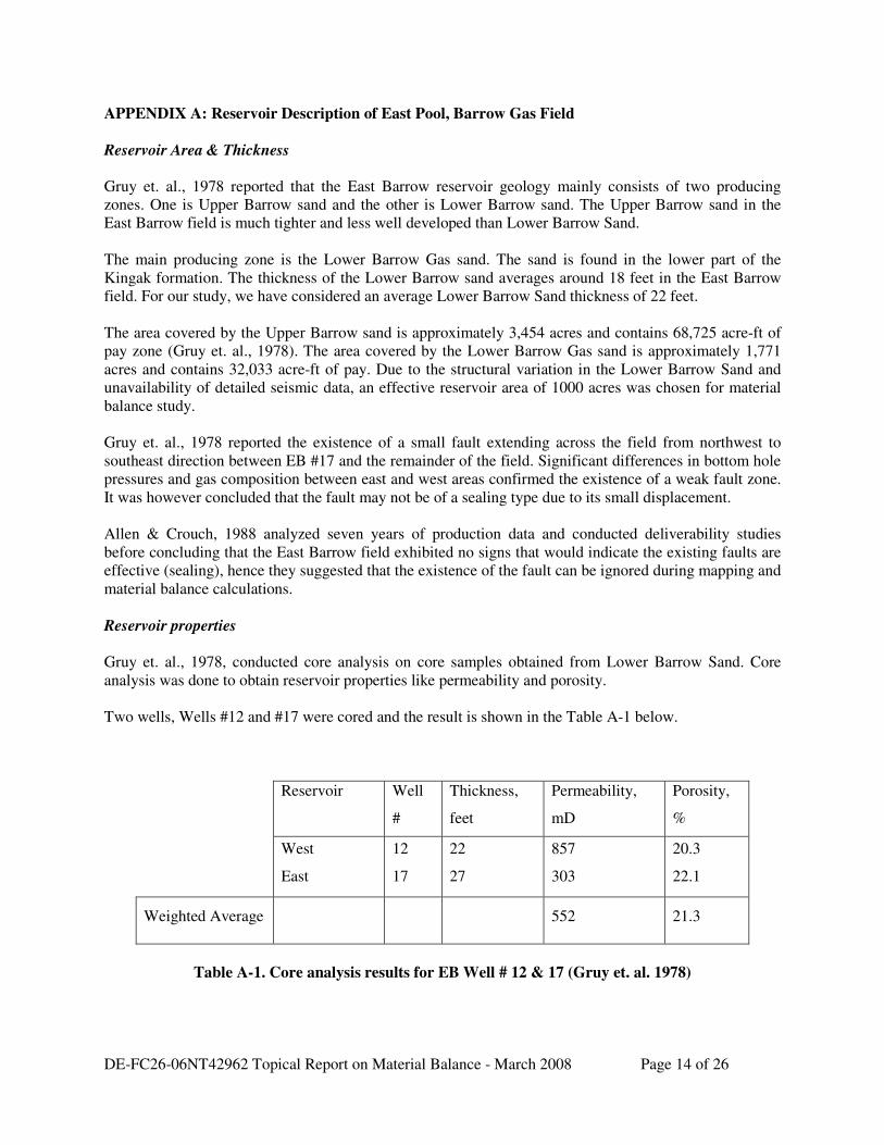
Two wells, Wells #12 and #17 were cored and the result is shown in the Table A-1 below.

Reservoir Well

#

Thickness,

feet

Permeability,

mD

Porosity,

%

West

East

12

17

22

27

857

303

20.3

22.1

Weighted Average 552 21.3

Table A-1. Core analysis results for EB Well # 12 & 17 (Gruy et. al. 1978)


The permeability results obtained from core analysis seems to be very large and possibly erroneous. Gruy

et. al., 1978 further conducted well testing analysis and obtained permeability in the range of 30-40 mD.

Hence with an element of doubt over reservoir permeability, an average reservoir permeability of 100mD

was chosen for conducting material balance study. The entire reservoir was considered isotropic with

uniform permeability in both horizontal and vertical directions.

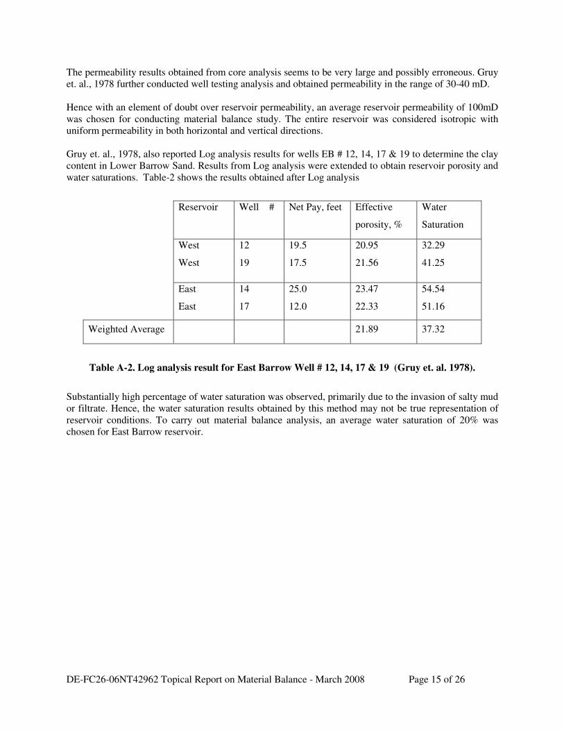
Gruy et. al., 1978, also reported Log analysis results for wells EB # 12, 14, 17 & 19 to determine the clay

content in Lower Barrow Sand. Results from Log analysis were extended to obtain reservoir porosity and

water saturations. Table-2 shows the results obtained after Log analysis

Reservoir Well # Net Pay, feet Effective

porosity, %

Water

Saturation

West

West

12

19

19.5

17.5

20.95

21.56

32.29

41.25

East

East

14

17

25.0

12.0

23.47

22.33

54.54

51.16

Weighted Average 21.89 37.32

Table A-2. Log analysis result for East Barrow Well # 12, 14, 17 & 19 (Gruy et. al. 1978).

Substantially high percentage of water saturation was observed, primarily due to the invasion of salty mud

or filtrate. Hence, the water saturation results obtained by this method may not be true representation of

reservoir conditions. To carry out material balance analysis, an average water saturation of 20% was

chosen for East Barrow reservoir.


Reservoir Pressure and Temperature

Gruy et. al., 1978, performed reservoir pressure buildup test in East Barrow wells #17 and #19. The

results shows that the original bottomhole pressure corrected to a datum of -2000 ft was found to be 1008

psia in east block in well #17 and 994 psi in the west fault block at the same datum in the well #19.

However, according to Allen and Crouch, 1988 report, the existence of fault line has no impact on the

overall performance of the reservoir. Keeping this in mind an average initial reservoir pressure of 1010

psi is considered for material balance study.

Gruy et. al., 1978, conducted bottomhole thermometer runs in South Barrow well # 13 and obtained a

reservoir temperature of 620F. However, since no similar tests were conducted in East Barrow gas

reservoir, this temperature cannot be assumed as initial reservoir temperature. Bottomhole temperature

gradient data obtained from North Slope Borough files for well EB #14 (1987), #19 (1996) & #21 (1996)

suggest that the bottomhole temperature is around 450F. Moreover, PRA in their 2007 engineering report

presented static temperature gradient for East Barrow wells #15 and #21. They obtained an average static

reservoir temperature of 500F.

Taking an average of available bottomhole temperature data and accounting for the cooling effect caused

due to continuous gas production (Joule’s Thompson effect), an average bottomhole temperature of 500F

is finally chosen as initial reservoir temperature.

Original Gas in Place (OGIP)

Gruy et. al., 1978, conducted material balance analysis to calculate initial gas in place by assuming a

volumetric gas reservoir and utilizing core and log analysis data. The reservoir was assumed to reduce to

a pressure of 235 psia. The recovery factor obtained for Lower Barrow sand is estimated to be 77%. The

Original Gas in Place (OGIP) calculated for Lower Barrow Sand is around 15 MMMCF.

In contrast to previous conclusions, Allen & Crouch 1988, reported the OGIP to be around 6.5 MMMCF.

They included the impact of strong water influx while estimating the initial gas reserves by water influx

calculations. They reported that by the end of 1988 about 91% of OGIP has already been recovered and

the rest shall be recovered within the next 2.5 years.

PRA 2007, however performed pressure tests and concluded that the reservoir pressure was 935 psia and

gas production continued with negligible water production. The reservoir has actually produced for a

much longer time than predicted for water driven mechanism. Interestingly, around 8 MMMCF of gas has

already been produced from the reservoir. This figure is much higher than previously estimated by Allen

and Crouch, 1988. PRA, 2007, explained this behavior by making a hypothesis that the reservoir pressure

stabilized due to possible gas recharge from insitu hydrates.

As the probability of finding insitu hydrates within Lower Barrow sands cannot be ruled out, thus at this

stage no estimate has been made about the OGIP for current material balance studies. This shall be

estimated by conducting detailed reservoir characterization.

Water Influx

Gruy et. al., 1978, reported presence of oil water contact below the East Barrow gas reservoir. They

concluded that the reservoir drive mechanism is primarily gas driven with negligible water influx.

However Allen and Crouch, 1988, conducted detailed water influx study based on seven years of

production history data and claimed that the entire reservoir shall be watered out by the end of 1990.


According to Allen & Crouch, 1988, the reservoir was under strong aquifer support. In contrast to

previous studies currently (2007), the reservoir is producing negligible amount of water and no well has

been plugged in due to excessive water production. Hence, the impact of an associated aquifer cannot be

claimed with certainty. Hence, for material balance study, water influx is studied as a separate scenario to

gauge its impact on reservoir performance.

Production Data

Production data constitutes a very important aspect of material balance study. PRA collected production

history data for each East Barrow well. Production data for each well is available from December 1st,

1981. The production data was logged on a monthly basis for each well and included information such as

well number, well type, gas production rate, water production rate, production days and reporting days.

This information can be extended easily to generate data like cumulative gas production and water

production with time. PRA merged the individual well data and provided a consolidated production

history data for East Barrow Pool from December 1, 1981 through May 1, 2007.

Unfortunately flowing bottomhole pressures were not reported on a regular basis. However Allen &

Crouch, 1988, reported several well shut in pressures between 1981 and 1988. Recently PRA 2007,

submitted their report on engineering study of East Barrow reservoir, they reported an average reservoir

pressure as observed on May 01, 2007. As these shut in pressures may not represent the reservoir

pressures, the actual average reservoir pressure may be within +/- 20% of the reported data. This vital

piece of information was included as part of production history data.

As expected, gas production rate never remained constant for the reservoir and hence we will have to

make some assumptions while conducting material balance analysis with water influx and hydrate

dissociation simulation studies.


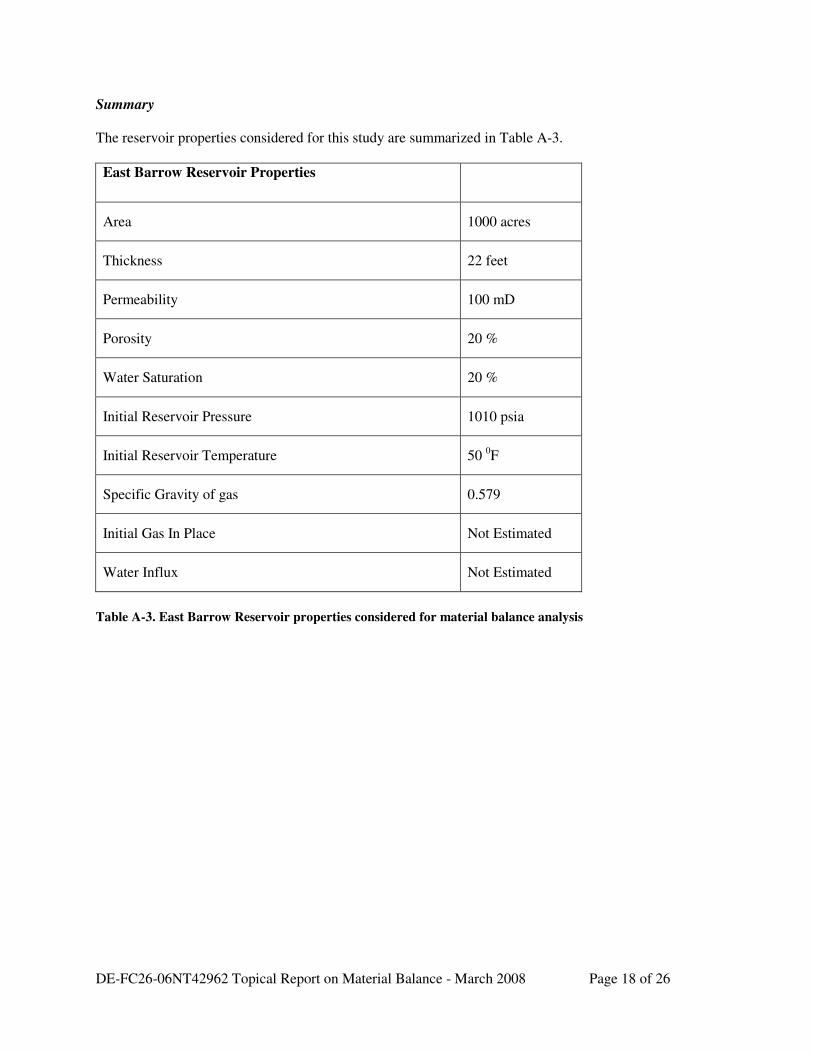
Summary

The reservoir properties considered for this study are summarized in Table A-3.

East Barrow Reservoir Properties

Area 1000 acres

Thickness 22 feet

Permeability 100 mD

Porosity 20 %

Water Saturation 20 %

Initial Reservoir Pressure 1010 psia

Initial Reservoir Temperature 50 0F

Specific Gravity of gas 0.579

Initial Gas In Place Not Estimated

Water Influx Not Estimated

Table A-3. East Barrow Reservoir properties considered for material balance analysis


APPENDIX B: Extended Material Balance Technique by West & Cochrane, 1994

Introduction

Tight, shallow gas reservoirs present a number of unique challenges in determining reserves accurately.

Traditional methods such as decline analysis and material balance are inaccurate due to the formation’s

low permeability and the usually poor-quality pressure data. The low permeabilities cause long transient

periods that are not separated early from production decline with conventional decline analysis, resulting

in lower confidence in selecting the appropriate decline characteristics which effect recovery factors and

remaining reserves significantly.

West and Cochrane, 1994, used the Medicine Hat Field in western Canada as an example of these types of

reservoirs and developed a methodology, called the Extended Material Balance technique, to evaluate gas

reserves. The Medicine Hat Field is a tight, shallow gas reservoir producing from multiple highly

interbedded, silty sand formations with poor permeabilities of less than 0.1 md. This poor permeability is

the main characteristic of these reservoirs that affects conventional decline analysis. Due to these low

permeabilities, wells experience long transient periods before they begin experiencing pseudosteady state

flow that represents the decline portion of their lives. One of the principal assumptions often neglected

when conducting decline analysis is that the pseudosteady state must have been achieved. The initial

transient production trend of a well or group of wells is not indicative of the long-term decline of the well.

Another characteristic of tight, shallow gas reservoirs that affects conventional decline analysis is that

constant reservoir conditions, an assumption required for conventional decline analysis, do not exist

because of increasing drawdown, changing operating strategies, erratic development, and deregulation.

Material balance is affected by tight, shallow gas reservoirs because the pressure data is limited, of poor

quality, and non-representative of a majority of the wells. In addition, pressure monitoring has been very

inconsistent. Varied measurement points (downhole or wellhead), inconsistent shut-in times, and different

analysis types (e.g., buildup and static gradient) make quantitative pressure tracking difficult. Both these

problems result in a scatter of data, which makes material balance extremely difficult.

West and Cochrane, 1994, developed an iterative methodology, called extended material balance “EMB”,

to determine gas reserves in 2300 wells in the Medicine Hat Field. East Barrow reservoir is a shallow gas

reservoir accompanied by lower reservoir pressures and poor reservoir permeability, this reservoir seems

to have features very similar to Medicine Hat Field. Scarcity and poor quality of pressure data and

inconsistencies in downhole pressure measurements make this field a perfect candidate for applying

Extended Material Balance analysis as proposed by West and Cochrane, 1994.

Methodology

Use of EMB method on East Barrow reservoir makes few fundamental assumptions

(1) The gas pool depletes volumetrically (i.e., no water influx) and

(2) All wells behave like an average well with the same deliverability constant, turbulence constant, and

BHFP.

The EMB technique is essentially an iterative process for obtaining a suitable p/Z vs. Gp line for a

reservoir where pressure data is inadequate. It combines the principles of volumetric gas depletion with

the gas deliverability equation. The deliverability equation for radial flow of gas describes the relationship

between the pressure differential in the wellbore and the gas flow rate from the well.

Qg = C [ P2

r - P2

wf ]n (1)


Where, Qg – gas production rate, MSCF/Day

Pr – average reservoir pressure, psia

Pwf – bottomhole flowing pressure, psia

n – flow exponent

Assuming low production rates from the wells, a laminar flow regime exists which can be described with

an exponent n = 1. The terms making up the coefficient C in equation-1 are either fixed reservoir

parameters (kh, re, rw, and T) that do not vary with time or terms that fluctuate with pressure,

temperature, and gas composition, i.e., µg and Z. The performance coefficient C is given by

C = kh 1422 TµgZ [ln(re/rw) − 0. 5] (2)

Where, C – deliverability coefficient, SCF/Day/psi2

k – reservoir permeability, mD

h – reservoir pay zone thickness, fts

T – temperature, 0F

Z – gas deviation factor at a give reservoir pressure

µ – gas viscosity, cp

re – reservoir radius, fts

rw – wellbore radius, fts

As the differences between initial and current reservoir pressures are not significant, the variation in the

pressure-dependent properties assumed to be negligible. Hence, C may be considered constant for a given

East Barrow gas reservoir over its life. With these simplifications, the deliverability equation becomes

Qg = C [ P2

r - P2

wf ] (3)

The sum of the instantaneous production rates with time will yield the relationship between Gp and

reservoir pressure, similar to the material balance equation. By use of this common relationship, with the

unknowns being initial free gas in place G and the performance coefficient C, the EMB method involves

successive iterations to find the correct p/Z vs. Gp relationship in order to achieve a constant (horizontal

line ) C with time. The proposed iterative method is applied as outlined in the following steps

Step 1: Using gas average specific gravity, initial reservoir pressure and constant reservoir temperature

(considering isothermal conditions), calculate the gas deviation factor Z based on Dranchuk and

Abou Kassem equation of state described in Craft & Hawkins, 1990 ed. Obtain Z factor as a

function of pressure and plot P/Z vs. P on a Cartesian scale.

Step 2: Using material balance equation, for volumetric gas reservoir (Craft & Hawkins, 1990), an initial

estimate for p/Z variation with Gp is made by putting the known initial pressure Pi and guessing

initial gas in place G in the equation

p/Z =pi/Zi − [m]Gp (4)

with the slope m as defined by

m = (Pi/Zi)/G (5)

Where, P – reservoir pressure at a particular time, psia

Z – corresponding gas deviation factor

Pi – initial reservoir pressure, psia

Zi – gas deviation factor at initial reservoir pressure


m – slope, psi/SCF

Gp – cumulative gas production, SCF

G – initial gas in place, SCF

Step 3: The p/Z versus time relationship is established by simply substituting the actual cumulative

production Gp into the material balance equation, other terms in the equation like slope m, initial

pressure Pi and cumulative gas production Gp is known. The reservoir pressure P can now be

generated as a function of time from the plot of p/Z as a function of p, i.e., step 1.

Step 4: No information is available about well’s bottomhole flowing pressure in the production history

data. To obtain a deliverability equation for East Barrow gas reservoir, four point deliverability

data from PRA 2007 report was used. Pseudosteady state is considered and a correlation is

developed to relate reservoir pseudo pressures, pseudo bottomhole pressure with gas production

rate. To obtain pseudo reservoir pressures from available pressure data and to convert the

calculated pseudo bottomhole pressure, gas viscosity and Z factor data are used. Gas viscosity

calculations are performed by using correlation developed by Lee, Gonzalez & Eakin (Craft &

Hawkins, 1990).

Bottomhole flowing pressure was calculated for corresponding reservoir pressure using the

deliverability equation and properties i.e. viscosity and Z factor.

Step 5: Knowing the actual production rates, Qg and BHFPs (Pwf) for each monthly time interval, and

having estimated the reservoir pressures P from step 3, C is calculated for each time interval by

rearranging Equation 3 as

C = Qg / [P2 − Pwf

2] (6)

Step 6: C is plotted versus time. If C is not constant (i.e. the plot is not a horizontal line), a new P/Z

versus Gp is guessed and the steps 2, 3 and 5 are repeated.

Step 7: Once a constant C solution is obtained, the representative P/Z relationship has been defined for

reserves determination.


APPENDIX C: Water Influx Model by Pletcher, 2002 and Ahmed & McKinney, 2005

Introduction

The plot of p/Z versus cumulative gas production Gp is a widely accepted method for solving gas material

balance under depletion drive conditions. The extrapolation of the plot to atmospheric pressure provides a

reliable estimate of the original gas-in-place. If a water drive is present the plot often appears to be linear,

but the extrapolation will give an erroneously high value for gas-in-place. If the gas reservoir has a water

drive, then there will be two unknowns in the material balance equation, even though production data,

pressure, temperature, and gas gravity are known. These two unknowns are initial gas-in-place (G) and

cumulative water influx (We). In order to use the material balance equation to calculate initial gas-in-

place and aquifer size, an independent method of estimating the cumulative water influx We, has been

developed (Pletcher, 2002, Ahmed & McKinney, 2005).

Material balance equation for a volumetric reservoir can be modified to include the effect of water influx.

Assuming a reservoir under active water drive, in presence of an associated aquifer, the material balance

equation for an isothermal reservoir can be written as,

G(Bg − Bgi) + We = GpBg + WpBw (7)

Where, G – initial gas in place, SCF

We – cumulative water influx, cuft


Bg – gas formation volume factor, cu ft / SCF at a given pressure P

Bgi - gas formation volume factor, cu ft / SCF at initial pressure Pi

Bw - water formation volume factor, cu ft / SCF at a given pressure P

The above equation can be arranged and expressed as:

(GpBg + WpBw)/(Bg − Bgi) = G + We/(Bg − Bgi) (8)

Pletcher, 2002 & Ahmed et. al., 2005 proposed plotting (GpBg + WpBw)/(Bg − Bgi), on the y-axis vs.

cumulative gas production (Gp) on the x-axis (Equation 8). If the reservoir is depletion drive (i.e., no

water influx), the water influx term (We) goes to zero, Equation - 9 and the points plot in a horizontal line

with the y-intercept equal to the original gas in place (OGIP), G.

(GpBg + WpBw)/(Bg − Bgi) = G + 0 (9)

If a water drive is present, the water influx term is not zero, and the points will plot above the depletion-

drive line (above G) with some type of slope. In other words, the existence of a sloping line vs. a

horizontal line is a valuable diagnostic tool for distinguishing between depletion drive and water drive.

Pletcher, 2002, in the paper sighted that the sloping water drive line can be extrapolated back to the y-

intercept to obtain the original gas in place (OGIP). However, the slope usually changes with each plotted

point; thus, the correct slope for extrapolation is very difficult, if not impossible, to establish, so this

method for estimating OGIP is not recommended.

The graphical technique can be further used to estimate the value of We, because at any time the

difference between the straight line (GpBg + WpBw)/(Bg − Bgi) and horizontal line (G) will give the

value of We/(Bg − Bgi). Moreover, the cumulative water influx (We) result can be extended to estimate

the size of associated aquifer.


The effectiveness of this method lies in its ability to provide qualitative information about the

performance of gas reservoir producing under aquifer support. The nature of the slope also helps in

identifying aquifer strength (Pletcher, 2002). High positive slopes are associated with strong water drives

whereas weak water drive has negative slope (Pletcher, 2002). The comparison although is purely

qualitative, still provides vital information about the aquifer size and type without quantifying it.

Methodology

To understand the behavior of East Barrow reservoir, an assumption is made that the gas reservoir is

under the influence of constant water influx from an aquifer. The associated aquifer is strong enough to

supply required amount of water to maintain the observed pressure response. Graphical technique

proposed by Pletcher, 2002, Ahmed & McKinney, 2005, shall be used to test the East Barrow reservoir in

presence of aquifer support and in this process estimate unknown parameters like initial gas in place,

cumulative water influx and aquifer size. The effect of aquifer support shall be qualitatively judged using

this technique. The entire exercise shall be a test on the production data to investigate the impact of

aquifer support, if any. In order to use water influx model, i.e. the graphical technique, following steps are

followed.

Step 1: Use Dranchuk and Abou Kassem equation of state, (described in Craft & Hawkins, 1990) to

generate Z-factor for corresponding pressures starting from reservoir initial pressure of 1010 psi.

Plot Z vs. Pressure plot and develop a linear correlation between the two parameters.

Step 2: Generate Z factor and gas formation volume factors, Bg for reservoir shut in pressures available in

the production data.

Step 3: Develop (GpBg + WpBw)/(Bg − Bgi) term by using production data. The term is time dependent,

hence generate (GpBg + WpBw)/(Bg − Bgi) as a function of Gp for available reservoir shut in

pressure, P.

Step 4: Draw a best possible slope through the data set.

Step 5: If the slope is zero (horizontal) then the reservoir is volumetric. Stop the calculations.

Step 6: If the slope is not zero, the reservoir is under active water drive, the strength of the water drive can

be qualitatively gauged by studying the slope.

Step 7: The slope cuts the y-axis at Gp = 0, that can be considered as the apparent OGIP G value for this

case. However, as discussed, this may not be an accurate estimate.

Step 8: To find the cumulative water influx, We from known OGIP (obtained above), subtract G from

(GpBg + WpBw)/(Bg − Bgi) and multiply the same by (Bg − Bgi).

Step 9: Calculate aquifer size by considering water and formation compressibility.


APPENDIX D: Hydrate Material Balance Model by Gerami & Darvish, 2006

Introduction

The geologic occurrence of gas hydrate has been known since the mid-1960s when gas hydrate

accumulations were discovered in Russia. Vast amount of hydrocarbon are estimated to be trapped in

hydrate deposits around the world (Sloan, 1998). Such deposits exist in distinct geologic formations such

as permafrost and deep marine sediments. The North Slope of Alaska has large areas of potential hydrate

deposits due to the environment of pressure and temperature within hydrate stability conditions.

Gerami & Darvish, 2006, developed a material balance model for hydrate capped reservoirs. This model

differs from conventional volumetric (depletion drive) and waterdrive type material balance models

because it includes the effect of gas generated from hydrate decomposition and related cooling effect. The

material balance equation has been developed by analytically and simultaneously solving the mass and

energy balance equations. The solution yields the average reservoir pressure and the gas generated from

hydrate decomposition as a function of cumulative gas production, for a reservoir that is produced at a

constant rate.

Hydrate dissociation is an endothermic process, gas production reduces reservoir pressure and triggers

hydrate dissociation leading to reduction in reservoir temperatures. Gas property changes continuously

due to changing pressure and temperature conditions. Gerami & Darvish 2006, considered these effects

while developing material balance model for hydrate capped systems. Their paper assumes important

requirement before carrying out material balance analysis. These assumptions are mentioned below.

1. A tank type model considered for the study implying that the temperature and pressure within the

reservoir are instantaneously uniform and are therefore only function of time.

2. Geothermal and hydrostatic gradient ignored.

3. Kinetics of hydrate decomposition neglected.

4. Reservoir is comprised of hydrates, water and gas. Reservoir considered volumetric (no water

influx).

5. Free gas temperature remains at the initial reservoir temperature.

6. The thermo-physical properties of hydrate, the reservoir, and surrounding formation (cap and

base rocks) remain constant during the production period.

Under these assumptions Gerami & Darvish, 2006, modified the gas material balance equation and

presented the following equation for hydrate-free gas system.

Pavg(t)/Z(t) = (Pi/Zi){1-(Gp(t) – Gg(t))/Gf} (10)

Pavg – average reservoir pressure at a given time, psia

Pi – initial reservoir pressure, psia

Zi – gas deviation factor at Pi

Z – gas deviation factor at Pavg


Gg – cumulative gas generation (from hydrate dissociation), SCF

Gf – initial free gas in place, SCF

To develop an equation to obtain temperature as a function of time, energy balance calculations were

performed. The governing equation of heat transfer is determined by conservation of energy using

Fourier’s law of conduction. Suitable boundary condition is imposed on the heat equation and energy

balance equation is also developed (Gerami & Darvish, 2006).


Hydrate block temperature is represented by a general equation given below,

Tse(t) = Ti – b(t)t ( Tse >= 32 0F) (11)

Where, Tse – hydrate cap temperature, 0F

Ti – initial reservoir temperature, 0F

b(t) – hydrate cap temperature parameter, 0F

It is assumed that the slow dissociation rates causes hydrate zone pressure to be in equilibrium with

reducing temperature. The changing temperature is related to the reservoir pressure by empirical equation

given by Kamath & Holder, 1987, for estimating hydrate equilibrium pressure and temperature. The

correlation was developed to estimate the hydrate stability zone in North Slope, Alaska.

P = exp(38.98-8533.80/Tse) (12)

The equations presented above are solved simultaneously to obtain hydrate cap temperature parameter

(b(t)) (Gerami & Darvish, 2006). The b(t) parameters combines the effect of hydrate dissociation and gas

production rate to estimate the temperature profile. The hydrate cap temperature parameter b(t) is a strong

function of gas production rate, reservoir volume, thermophysical properties of hydrate cap and a weak

function of production time. This temperature profile is used to obtain the reservoir pressure using

equation-12. The obtained pressure profile can then be easily compared with the production history data.

Gerami & Darvish, 2006, hydrate material balance model can be used an engineering tool for evaluating

the role of hydrates in improving the productivity and extending the life of hydrate capped gas reservoir.

Moreover, after careful validation of the model with production history data, the model can be used as a

predictive tool to estimate parameters like initial free gas in place, hydrate thickness etc.

Methodology

East Barrow gas field is a shallow gas reservoir, with an average reservoir depth around 2000’ and

reservoir temperature in the range of 500F. Previous work (Walsh et. al, 2007) has interpreted the

existence of hydrate stability zone within the East Barrow gas reservoir. Recently proposed material

balance model for hydrate capped free gas reservoir (Gerami & Darvish, 2006) has been adopted to

understand the performance expected from a hydrate associated gas reservoir.

A stepwise procedure is laid out with an aim to apply hydrate model to East Barrow gas reservoir.

Step 1: Model Validation

To carry out model validation, a gas tank was considered. The areal extent of the reservoir was

considered to be 8 acres whereas the thickness of the reservoir was considered very large (semi-

infinite system). All other reservoir properties were assumed the same as considered for East

Barrow reservoir (refer data and assumptions). The material balance exercise was performed at a

constant production rate of 5 MSCF/Day. The calculations were performed for a small production

period. This was done with an aim to keep the reservoir pressure fairly high. No temperature and

pressure gradient was considered for this case. No hydrate zone thickness was considered in this

case.


Based on the assumptions, material balance exercise was carried out by considering a volumetric

(depletion drive) gas reservoir. P/Z relation was then plotted against Gp. Reservoir pressure was

also calculated by simultaneously estimating Z-factor.

The hydrate model was then modified after several attempts to obtain a material balance model

that accounts for temperature reduction within the reservoir. Although no hydrate cap was

considered for this case, still a hydrate layer of zero ft thickness was assumed. It was further

assumed that the initial reservoir pressure is controlled by this hydrate zone. Temperature change

in the reservoir was calculated by evaluating hydrate cap temperature parameter b(t) and equation

11. In absence of hydrate zone, parameter b(t) is purely a function of gas production rate and

reservoir volume and independent of time. Thus it remains constant for a volumetric model. Due

to the adiabatic behavior of the reservoir, the material balance equation is modified and

temperature terms are retained. The material balance equation evaluated for this step takes the

form

(13)

P/Z vs. Gp is plotted against Gp using modified Darvish model. The performance of two models

is compared. Under present circumstances Darvish model must show a close match with

volumetric model. This will validate the modified version of Darvish model (without hydrates).

After model validation, we can use the modified model to compare the performance against

original Darvish model (with hydrates) easily.

Step 2: The modified Darvish model was scaled up to match East Barrow reservoir properties (refer data

and assumptions). The actual production shows variable gas production rate. This violates the

application of modified Darvish model. To obtain a similar condition a constant gas production

rate was chosen (Qg = 1600 MSCF/Day). The scaled up reservoir was still considered to have no

insitu hydrates. Under this situation, modified Darvish model was applied to obtain P/Z vs. Gp

and Pressure vs. time plots.

Step 3: Original Darvish model is now used to obtain pressure response in presence of hydrate zone. East

Barrow type reservoir is produced at a constant rate of 1600 MSCF/Day. In this case however, the

hydrate cap temperature parameter b(t) becomes function of time as well. The parameter is used

to obtain the hydrate cap temperature, changing continuously with time. Being a thin reservoir

(22fts) the hydrate cap temperature is considered to be the reservoir temperature. Kamath and

Holder, 1987, empirical correlation is used to obtain the equilibrium pressure at the

corresponding temperature. For this case the hydrate equilibrium pressure is considered as the

reservoir pressure.

The impact of hydrate zone thickness on the performance of East Barrow type reservoir model is

studied by conducting Darvish material balance analysis for different hydrate zone thickness

(varying from 0.5 feet to 22 feet).

National Energy Technology Laboratory 626 Cochrans Mill Road P.O. Box 10940 Pittsburgh, PA 15236-0940 3610 Collins Ferry Road P.O. Box 880 Morgantown, WV 26507-0880 One West Third Street, Suite 1400 Tulsa, OK 74103-3519 1450 Queen Avenue SW Albany, OR 97321-2198 2175 University Ave. South Suite 201 Fairbanks, AK 99709 Visit the NETL website at: www.netl.doe.gov Customer Service: 1-800-553-7681

Oil & Natural Gas Technology - National Energy … Library/Research/Oil-Gas/methane... · Oil &...

Documents

Transcript of Oil & Natural Gas Technology - National Energy … Library/Research/Oil-Gas/methane... · Oil &...