Rate Transient Analysis and Flowing Material Balance for ... · Rate Transient Analysis and Flowing...

POLITECNICO DI TORINO

Department of Environment, Land and Infrastructure Engineering

Master of Science in Petroleum Engineering

Rate Transient Analysis and Flowing Material Balance for Oil & Gas Reservoir

Supervisor Prof. Dario Viberti Co-Supervisor: Prof. Alberto Guadagnini Dott. Muhammad Shoaib

Candidate:

Mohamed Amr Mohamed Abdelhamid Aly [S236320]

July 2018

I

Acknowledgement

“We raise to degrees whom We please, but over all those endowed with knowledge is the All-Knowing (Allah).” Quran surah Yusuf 76 (QS 12: 76)

“You have been given of knowledge nothing except a little.”

Quran surah Al Isra 85 (QS 17: 85)

All praises to ALLAH for the strength he gave to me and his blessings to complete my thesis. My extreme gratitude goes to my supervisor Prof. Dario Viberti for giving me the opportunity to work with him and for his continuous support and guidance through the whole Master of Science program. Over the course of this program I have gained a lot from his knowledge, advice and encouragement. I am also very thankful to the support I have received from my co-supervisor Prof. Alberto Guadagnini, for the time he has dedicated into helping me. Special thanks to Dott. Muhammad Shoaib for his help and the huge efforts he made with me to finish this work.

I would like to acknowledge both KAPPA software platforms, and

Schlumberger (SLB) for using the academic license of the rate transient analysis interface (Topaze NL) and (ECLIPSE) respectively in this work.

Finally, I would like to warmly thank my parents and my siblings for their endless support and love. Many thanks to my friends and colleagues who had encouraged me all the time during my studies.

II

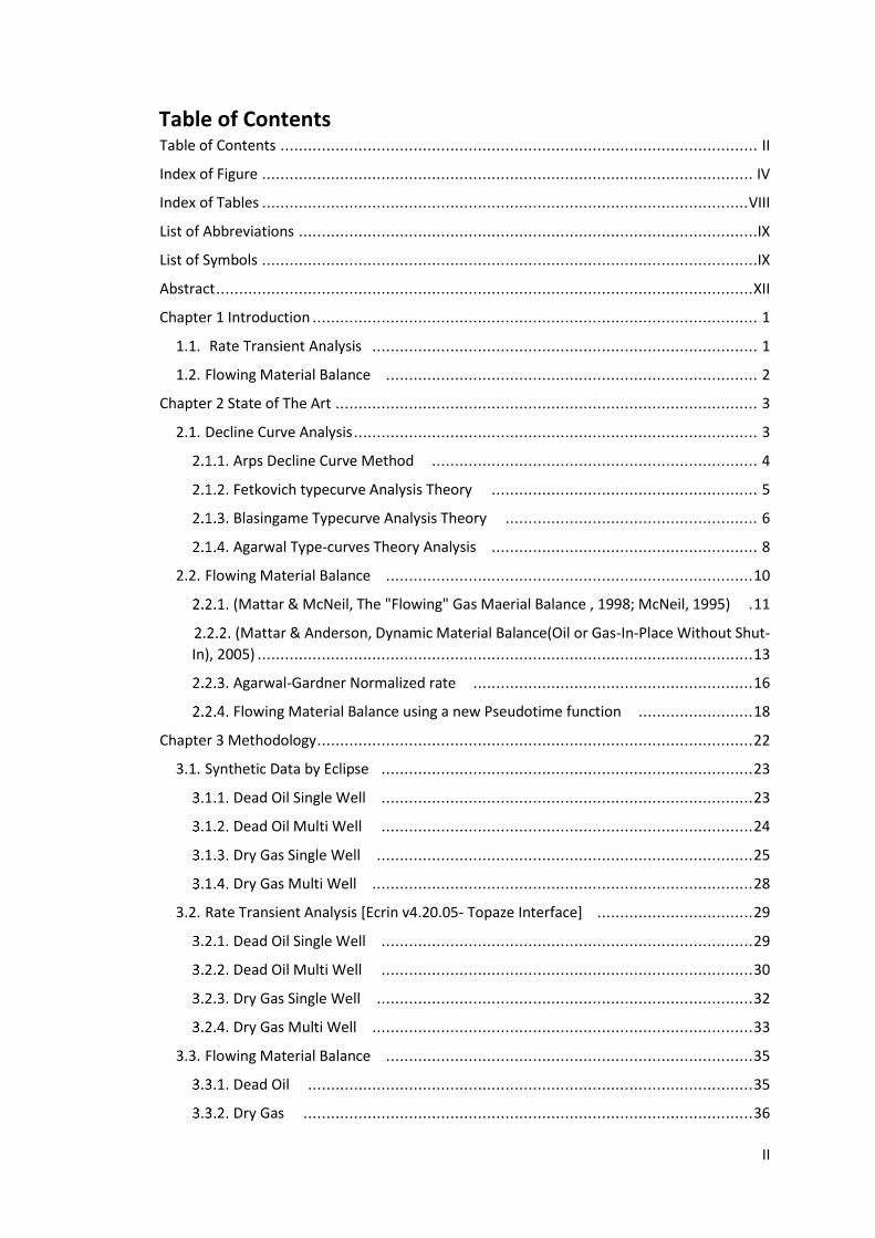
Table of Contents Table of Contents ........................................................................................................ II

Index of Figure ........................................................................................................... IV

Index of Tables .......................................................................................................... VIII

List of Abbreviations ....................................................................................................IX

List of Symbols ............................................................................................................IX

Abstract ..................................................................................................................... XII

Chapter 1 Introduction ................................................................................................. 1

1.1. .................................................................................... 1

1.2. Flowing Material Balance ................................................................................. 2

Chapter 2 State of The Art ............................................................................................ 3

2.1. Decline Curve Analysis ........................................................................................ 3

Arps Decline Curve Method ....................................................................... 4

Fetkovich typecurve Analysis Theory .......................................................... 5

Blasingame Typecurve Analysis Theory ....................................................... 6

Agarwal Type-curves Theory Analysis .......................................................... 8

2.2. Flowing Material Balance ................................................................................ 10

(Mattar & McNeil, The "Flowing" Gas Maerial Balance , 1998; McNeil, 1995) . 11

(Mattar & Anderson, Dynamic Material Balance(Oil or Gas-In-Place Without Shut-

In), 2005) ............................................................................................................ 13

Agarwal-Gardner Normalized rate ............................................................. 16

Flowing Material Balance using a new Pseudotime function ......................... 18

Chapter 3 Methodology ............................................................................................... 22

3.1. Synthetic Data by Eclipse ................................................................................. 23

Dead Oil Single Well ................................................................................. 23

Dead Oil Multi Well ................................................................................. 24

Dry Gas Single Well .................................................................................. 25

Dry Gas Multi Well ................................................................................... 28

3.2. Rate Transient Analysis [Ecrin v4.20.05- Topaze Interface] .................................. 29

Dead Oil Single Well ................................................................................. 29

Dead Oil Multi Well ................................................................................. 30

Dry Gas Single Well .................................................................................. 32

Dry Gas Multi Well ................................................................................... 33

3.3. Flowing Material Balance ................................................................................ 35

Dead Oil ................................................................................................. 35

Dry Gas .................................................................................................. 36

III

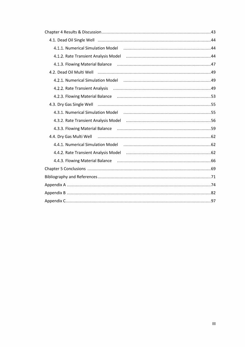
Chapter 4 Results & Discussion ..................................................................................... 43

4.1. Dead Oil Single Well ........................................................................................ 44

Numerical Simulation Model .................................................................... 44

Rate Transient Analysis Model .................................................................. 44

Flowing Material Balance ......................................................................... 47

4.2. Dead Oil Multi Well ........................................................................................ 49


Rate Transient Analysis ............................................................................ 49


4.3. Dry Gas Single Well ........................................................................................ 55




4.4. Dry Gas Multi Well ........................................................................................ 62




Chapter 5 Conclusions ................................................................................................ 69

Bibliography and References ........................................................................................ 71

Appendix A ................................................................................................................ 74

Appendix B ................................................................................................................ 82

Appendix C................................................................................................................. 97

IV

Index of Figure Figure 1: Nominal Decline at a point in time .................................................................... 4 Figure 2: How material balance time is used to change the variable rate scenario into

constant rate scenario (Fekete.com, Material Balance Time Theory) .................................. 7 Figure 3: Pi/zi plot as Parallel to Pwf/Z line in Pseudo Steady State Conditions. Flowing

Material Balance Approach. (Fekete.Com) .....................................................................11 Figure 4: (Ismadi, Kabir, & Hasan, 2012) Comparison of the two FMB approaches [Gas FMB

vs. Agarwal] for homogenous system. ...........................................................................17 Figure 5: Steps of Methodology done in this study ..........................................................22 Figure 6: Dead Oil Single Well Eclipse Model PVT data .....................................................24 Figure 7: Dead Oil Single Multi Well Model, Well Locations ..............................................24 Figure 8: Importing PVT data from Ecrin. Topaze database representing our model

parameters of Pressure and temperature ......................................................................26 Figure 9: Dry Gas Single Well Eclipse Model PVT data ......................................................27 Figure 10: Dry Gas Single Well Eclipse Model capillary pressure data ................................27 Figure 11: Dry Gas Multi Well Model, Well Locations ......................................................28 Figure 12: Dead Oil Single Well, Production rate and bottom hole flowing pressure vs. time29 Figure 13: Dead Oil Single Well PVT data input in Ecrin. Topaze ........................................29 Figure 14: Dead Oil Single Well Analytical Model Description ...........................................30 Figure 15: Dead Oil multi-well cumulative production vs. time .........................................30 Figure 16: Dead Oil Multi-well Model. Well location. ......................................................31 Figure 17: Dead Oil Multi-well Numerical Model description. ...........................................31 Figure 18: Dry Gas Single Well production and Bottom Hole Pressure Vs. Time ..................32 Figure 19: Dry Gas Single Well Analytical Model Description ............................................32 Figure 20: Dry Gas Multi-Well Cumulative production vs. time. ........................................33 Figure 21: Dry Gas Multi well Model. Well Locations. ......................................................33 Figure 22: Dry Gas Multi-well Numerical model Description .............................................34 Figure 23: Pseudo Pressure Function polynomial equation as a funcation of pressure .........37 Figure 24: Average Reservoir Pressure polynomial equation as a function of gas pseudo

pressure. ....................................................................................................................38 Figure 25: Average Reservoir Pressure Polynomial Equation as a Function of P/Z. ..............38 Figure 26: Gas Copressibility as a function of Pressure. ....................................................39 Figure 27: Gas Compressibility factor as a function of pressure. .......................................39 Figure 28: Gas viscosity as a function of pressure. ...........................................................40 Figure 29: Viscosity compressibility ratio as a function of cumulative production. ..............42 Figure 30: Dead Oil Single Well Production History Match. Rate, Cumulative production,

flowing pressure and model reservoir average pressure vs. Time. .....................................44 Figure 31: Dead Oil Single Well Log-Log Plot Match .........................................................44 Figure 32: Dead Oil Single Well Model Blasingame Plot Match. ........................................45 Figure 33: Dead Oil Single Well Model Fetkovich Plot Match. ...........................................45 Figure 34: Dead Oil Single Well Fetkovich Type-curves Match ..........................................46 Figure 35: Dead Oil Single Well Blasingame Type-curves Match. .......................................46 Figure 36: Dead Oil Single Well FMB, bpss is obtained as the Y-intercept of the straight line ..47 Figure 37: Dead Oil Single Well Flowing Material Balance using Oil Compressibility ............48 Figure 38: Dead Oil Single Well Flowing Material Balance using total Compressibility. .........48 Figure 39: Dead Oil Multi Well Cumulative Production vs. time. .......................................49

V

Figure 40: Dead Oil Multi-well Well #1 History Match. Rate, Cumulative production, flowing

pressure and model reservoir average pressure vs. Time. ................................................50 Figure 41: Dead Oil Multi-well Well #1 Log-Log Plot Match ..............................................50 Figure 42: Dead Oil Multi-well Well #1 Model Blasingame Plot Match. ..............................51 Figure 43: Dead Oil Multi-well Well #1 Model Fetkovich Plot Match. .................................51 Figure 44: Dead Oil Multi-well Well #1 Fetkovich Type-curves Match. ...............................52 Figure 45: Dead Oil Multi-well Well #1 Blasingame Type-curves Match. ............................52 Figure 46: Dead Oil Multi-well Well #1 FMB, bpss is obtained as the Y-intercept of the

straight line ................................................................................................................53 Figure 47: Dead Oil Multi-well Well #1 Flowing Material Balance using Oil Compressibility ..54 Figure 48: Dead Oil Multi-well Well #1 Flowing Material Balance using Total Compressibility.

.................................................................................................................................54 Figure 49: Dry Gas Single Well Well #4 History Match. Rate, Cumulative production, flowing

pressure and model reservoir average pressure vs. Time. ................................................56 Figure 50: Dry Gas Single Well Log-Log Plot Match. .........................................................56 Figure 51: Dry Gas Single Well Model Blasingame Plot Match. ..........................................57 Figure 52: Dry Gas Single Well Model Fetkovich Plot Match. ............................................57 Figure 53: Dry Gas Single Well Fetkovich Type-curves Match. ...........................................58 Figure 54: Dry Gas Single Well Blasingame Type-curves Match. ........................................58 Figure 55: Dry Gas Single Well FMB, bpss is obtained as the Y-intercept of the straight line ...59 Figure 56: Dry Gas Single Well, Gas Flowing Material Balance, P/z Plot. .............................60 Figure 57: Dry Gas Single Well, Agarwal Gardner Approach. .............................................60 Figure 58: Dry Gas Single Well, Using The New Pseudo Material Balance Function. .............61 Figure 59: Dry Gas Multi-well Well #1, Production Flow Rate & cumulative production vs.

Time. .........................................................................................................................62 Figure 60: Dry Gas Multi-well Well #1 History Match. Rate, Cumulative production, flowing

pressure and model reservoir average pressure vs. Time. ................................................63 Figure 61: Dry Gas Multi-well Well #1 Log-Log Plot Match. ..............................................63 Figure 62: Dry Gas Multi-well Well #1 Model Fetkovich Plot Match. ..................................64 Figure 63: Dry Gas Multi-well Well #1 Model Blasingame Plot Match. ...............................64 Figure 64: Dry Gas Multi-well Well #1 Fetkovich Type-curves Match. ................................65 Figure 65: Dry Gas Multi-well Well #1 Blasingame Type-curves Match...............................65 Figure 66: Dry Gas Multi-well Well #1 FMB, bpss is obtained as the Y-intercept of the straight

line ............................................................................................................................66 Figure 67: Dry Gas Multi-well Well #1, Gas Flowing Material Balance, P/z Plot. ..................66 Figure 68: Dry Gas Multi-well Well #1, Agarwal Gardner Approach. ..................................67 Figure 69: Dry Gas Multi-well Well #1 Using The New Pseudo Material Balance Function. ...67 Figure 70: Dead Oil Multi-well Well #2 History Match. Rate, Cumulative production, flowing

pressure and model reservoir average pressure vs. Time. ................................................82 Figure 71: Dead Oil Multi-well Well #2 Log-Log Plot Match. .............................................82 Figure 72: Dead Oil Multi-well Well #2 Model Blasingame Plot Match. ..............................83 Figure 73: Dead Oil Multi-well Well #2 Model Fetkovich Plot Match. .................................83 Figure 74: Dead Oil Multi-well Well #2 Fetkovich Type-curves Match. ...............................84 Figure 75: Dead Oil Multi-well Well #2 Blasingame Type-curves Match. ............................84 Figure 76: Dead Oil Multi-well Well #2 FMB, bpss is obtained as the Y-intercept of the

straight line. ...............................................................................................................85 Figure 77: Dead Oil Multi-well Well #2 Flowing Material Balance using Oil Compressibility ..85

VI

Figure 78: Dead Oil Multi-well Well #2 Flowing Material Balance using Total Compressibility

.................................................................................................................................86 Figure 79: Dead Oil Multi-well Well #3 History Match. Rate, Cumulative production, flowing

pressure and model reservoir average pressure vs. Time. ................................................87 Figure 80: Dead Oil Multi-well Well #3 Log-Log Plot Match. .............................................87 Figure 81: Dead Oil Multi-well Well #3 Model Blasingame Plot Match. ..............................88 Figure 82: Dead Oil Multi-well Well #3 Model Fetkovich Plot Match. .................................88 Figure 83: Dead Oil Multi-well Well #3 Fetkovich Type-curves Match. ...............................89 Figure 84: Dead Oil Multi-well Well #3 Blasingame Type-curves Match. ............................89 Figure 85: Dead Oil Multi-well Well #3 Well FMB, bpss is obtained as the Y-intercept of the

straight line ................................................................................................................90 Figure 86: Dead Oil Multi-well Well #3 Flowing Material Balance using Oil Compressibility ..90 Figure 87: Dead Oil Multi-well Well #3 Flowing Material Balance using Total Compressibility.

.................................................................................................................................91 Figure 88: Dead Oil Multi-well Well #4 History Match. Rate, Cumulative production, flowing

pressure and model reservoir average pressure vs. Time. ................................................92 Figure 89: Dead Oil Multi-well Well #4 Log-Log Plot Match. .............................................92 Figure 90: Dead Oil Multi-well Well #4 Model Blasingame Plot Match. ..............................93 Figure 91: Dead Oil Multi-well Well #4 Well Model Fetkovich Plot Match. .........................93 Figure 92: Dead Oil Multi-well Well #4 Fetkovich Type-curves Match. ...............................94 Figure 93: Dead Oil Multi-well Well #4 Blasingame Type-curves Match. ............................94 Figure 94: Dead Oil Multi-well Well #4 FMB, bpss is obtained as the Y-intercept of the straight

line. ...........................................................................................................................95 Figure 95: Dead Oil Multi-well Well #4 Flowing Material Balance using Oil Compressibility. .95 Figure 96: Dead Oil Multi-well Well #4 Flowing Material Balance using Total Compressibility.

.................................................................................................................................96 Figure 97: Dry Gas Multi-well Well #2 History Match. Rate, Cumulative production, flowing

pressure and model reservoir average pressure vs. Time. ................................................97 Figure 98: Dry Gas Multi-well Well #2 Log-Log Plot Match. ..............................................97 Figure 99: Dry Gas Multi-well Well #2 Model Fetkovich Plot Match. ..................................98 Figure 100: Dry Gas Multi-well Well #2 Model Blasingame Plot Match. .............................98 Figure 101: Dry Gas Multi-well Well #2 Fetkovich Type-curves Match. ..............................99 Figure 102: Dry Gas Multi-well Well #2 Blasingame Type-curves Match. ............................99 Figure 103: Dry Gas Multi-well Well #2 FMB, bpss is obtained as the Y-intercept of the

straight line .............................................................................................................. 100 Figure 104: Dry Gas Multi-well Well #2, Gas Flowing Material Balance, P/z Plot. .............. 100 Figure 105: Dry Gas Multi-well Well #2, Agarwal Gardner Approach. .............................. 101 Figure 106: Dry Gas Multi-well Well #2 Using The New Pseudo Material Balance Function.101 Figure 107: Dry Gas Multi-well Well #3 History Match. Rate, Cumulative production, flowing

pressure and model reservoir average pressure vs. Time. .............................................. 102 Figure 108: Dry Gas Multi-well Well #3 Log-Log Plot Match. ........................................... 102 Figure 109: Dry Gas Multi-well Well #3 Model Fetkovich Plot Match. .............................. 103 Figure 110: Dry Gas Multi-well Well #3 Model Blasingame Plot Match. ........................... 103 Figure 111: Dry Gas Multi-well Well #3 Fetkovich Type-curves Match. ............................ 104 Figure 112: Dry Gas Multi-well Well #3 Blasingame Type-curves Match. .......................... 104 Figure 113: Dry Gas Multi-well Well #3 FMB, bpss is obtained as the Y-intercept of the straight

line .......................................................................................................................... 105 Figure 114: Dry Gas Multi-well Well #3, Gas Flowing Material Balance, P/z Plot. .............. 105

VII

Figure 115: Dry Gas Multi-well Well #3, Agarwal Gardner Approach. .............................. 106 Figure 116: Dry Gas Multi-well Well #3 Using The New Pseudo Material Balance Function.106 Figure 117: Dry Gas Multi-well Well #4 History Match. Rate, Cumulative production, flowing

pressure and model reservoir average pressure vs. Time. .............................................. 107 Figure 118: Dry Gas Multi-well Well #4 Log-Log Plot Match. ........................................... 107 Figure 119: Dry Gas Multi-well Well #4 Model Fetkovich Plot Match. .............................. 108 Figure 120: Dry Gas Multi-well Well #4 Model Blasingame Plot Match. ........................... 108 Figure 121: Dry Gas Multi-well Well #4 Fetkovich Type-curves Match. ............................ 109 Figure 122: Dry Gas Multi-well Well #4 Blasingame Type-curves Match. .......................... 109 Figure 123: Dry Gas Multi-well Well #4 FMB, bpss is obtained as the Y-intercept of the straight

line .......................................................................................................................... 110 Figure 124: Dry Gas Multi-well Well #4, Gas Flowing Material Balance, P/z Plot. .............. 110 Figure 125: Dry Gas Multi-well Well #4, Agarwal Gardner Approach. .............................. 111 Figure 126: Dry Gas Multi-well Well #4 Using The New Pseudo Material Balance Function.111

VIII

Index of Tables

Table 1: Advantages and Disadvantages of Arps Decline Curve Analysis ............................. 4 Table 2: Comparison between Transient and Pseudo Steady State Conditions in Rate-Time

Type-curves, Based on Drainage Area A .......................................................................... 9 Table 3: Comparison between Transient and Pseudo Steady State Conditions in Rate-Time

Type-curves, Based on Effective Well Radius rwa2 ............................................................. 9

Table 4: Comparison between Transient and Pseudo Steady State Conditions in Rate-

Cumulative Production Type-curves, Based on Drainage Area A ........................................ 9 Table 5: Comparison between Transient and Pseudo Steady State Conditions in Rate-

Cumulative Production Type-curves, Based on Effective Well Radius rwa2 ..........................10

Table 6: Comparison between Transient and Pseudo Steady State Conditions in Cumulative

Production-Time Type-curves, Based on Effective Well Radius rwa2 ...................................10

Table 7: (Choudhury & Gomes, 2000) Gas in Place Estimates and the status of J sand .........12 Table 8: (Choudhury & Gomes, 2000) Comparison of Gas in Place estimates by different

methods ....................................................................................................................12 Table 9: (Guzman, Arevalo, & Espinola, 2014) Summary of OGIP (MMSCF) Calculation by

Different Studies .........................................................................................................13 Table 11: Flowing Material Balance Approach introduced by (Mohammed & Enty, 2013) ....21 Table 12: Dead Oil Singe Well Model Description ............................................................23 Table 13: Dry Gas Single Well Model Description ............................................................25 Table 14: Comparison between results obtained by Fetkovich Type-curves match and

Numerical Simulation Model. .......................................................................................46 Table 15: Dead Oil Single Well PVT Data used in RTA & FMB ............................................47 Table 16: Dead Oil Single Well, reservoir permeability using FMB approach. ......................47 Table 17: Dead Oil Single Well OOIP comparison between the different approaches. ..........49 Table 18: Dead Oil Multi-well Well #1 Well PVT Data used in RTA & FMB ..........................53 Table 19: Dead Oil Multi-well Well #1, reservoir permeability using FMB approach. ...........54 Table 20: Dead Oil Multi-well OOIP comparison between the different approaches. ...........55 Table 21: Dry Gas Single Well reservoir permeability using FMB approach. ........................59 Table 22: Dry Gas Single Well OGIP comparison between the different approaches. ...........61 Table 23: Dry Gas Multi-well Well #1, reservoir permeability using FMB approach. ............66 Table 24: Dry Gas Multi-well OGIP comparison between the different approaches. ............68 Table 25: Dead Oil Multi-well Well #2, reservoir permeability using FMB approach. ...........85 Table 26: Dead Oil Multi-well Well #3, reservoir permeability using FMB approach. ...........90 Table 27: Dead Oil Multi-well Well #4, reservoir permeability using FMB approach. ...........95 Table 28: Dry Gas Multi-well Well #2, reservoir permeability using FMB approach. .......... 100 Table 29: Dry Gas Multi-well Well #3, reservoir permeability using FMB approach. .......... 105 Table 30: Dry Gas Multi-well Well #4, reservoir permeability using FMB approach. .......... 110

IX

List of Abbreviations DCA Decline Curve Analysis

DMB Dynamic Material Balance

FBHP Flowing Bottom Hole Pressure

FMB Flowing Material Balance

MBE Material Balance Equation

PA Production Analysis

Pavg Average Reservoir Pressure

PDA Production Data Analysis

PDG Permanent Downhole Gauges

PTA Pressure Transient Analysis

PVT Pressure Volume Temperature

RTA Rate Transient Analysis

List of Symbols

(𝒕)𝒄 Characteristic time (second)

𝒄𝒈̅̅ ̅ Gas compressibility at average (static) reservoir pressure (psia-1)

𝝁𝒈̅̅̅̅ Gas viscosity at average (static) reservoir pressure (cp)

𝑩𝒈 Gas Formation Volume factor (SCF/STB)

𝑩𝒐 Oil Formation Volume Factor (bbl/ STB)

𝑪𝑨 Dietz shape Factor (-)

𝑮𝒑 Cumulative gas production (MSCF)

𝑮𝒑𝒏 Normalized pseudo cumulative function (MSCF)

𝑵𝒑 Cumulative oil production (STB)

𝑵𝒑𝒂 Ultimate recovery (STB)

𝑷𝒔𝒄 Pressure at standard conditions (psia)

𝑷𝒕𝒉 Tubing head pressure (psia)

𝑸𝑫𝑨 Dimensionless cumulative production based on area A (-)

𝑸𝒂𝑫 Dimensionless cumulative production based on rwa2 (-)

𝑺𝒈𝒊 Initial Gas saturation (-)

𝑻𝒂 New Material Balance Pseudo time function (second)

𝑻𝒔𝒄 Temperature at standard conditions (R)

𝑽𝑷 Pore Volume (ft3)

𝒁𝒊 Initial gas compressibility factor (-)

X

𝒃𝒂,𝒑𝒔𝒔 Pseudo steady state constant for gas (psia/MSCF/s)

𝒃𝒑𝒔𝒔 Pseudo steady state constant for oil (psia/STB/s)

𝒄𝒈 Gas Compressibility (psia -1)

𝒄𝒈𝒊 Initial gas Compressibility (psia -1)

𝒄𝒐 Oil Compressibility (psia -1)

𝒄𝒐𝒊 Initial Oil compressibility (psia -1)

𝒄𝒕 Total Compressibility (psia -1)

𝒄𝒕𝒊 Initial total compressibility (psia -1)

𝒎(𝒑𝒊) Initial reservoir pseudo pressure function (psia2/cp)

�̅� Reservoir Static (Average) Pressure (psia)

𝒑𝑫 Dimensionless Pressure (-)

𝒑𝒊 Initial Pressure (psia)

𝒑𝒘𝑫 Dimensionless wellbore pressure used by Agarwal (-)

𝒑𝒘𝑫′ Dimensionless wellbore pressure derivative used by Agarwal (-)

𝒑𝒘𝒇 Bottom hole Flowing Pressure (psia)

𝒒𝑫𝒅 Fetkovich Dimensionless rate (-)

𝒒𝒈 Gas flow rate at surface conditions (MSCF/d)

𝒒𝒐 Oil flow rate at stock tank (STB/d)

𝒓𝑫 Dimensionless diameter (-)

𝒓𝒆 Drainage radius (ft)

𝒓𝒆𝑫 Dimensionless outer diameter (-)

𝒓𝒘 Wellbore radius (ft)

𝒓𝒘𝒂 Effective Wellbore radius (ft)

𝒕𝑫 Dimensionless time (-)

𝒕𝑫𝑨 Dimensionless time based on the drainage area (-)

𝒕𝑫𝒅 Fetkovich Dimensionless time (-)

𝒕𝒄 Material Balance time for oil (second)

𝒕𝒄𝒂 Material Balance pseudo time function for gas (second)

𝒕𝒄𝒈 Material Balance time for gas (second)

𝒕𝒔 Stabilization time (second)

𝝁𝒈 Gas Viscosity (cp)

XI

𝝁𝒈𝒊 Initial gas Viscosity (cp)

𝝁𝒐 Oil Viscosity (cp)

∆𝒑 Pressure difference between initial and bottom hole flowing pressures (psia)

𝑩 Formation Volume Factor (bbl/STB)

𝑫 Nominal decline rate (second-1)

𝑭 MBH Function (-)

𝑮 Initial Gas In-Place (MSCF)

𝑵 Initial Oil In-Place (STB)

𝑺 Skin (-)

𝑻 Reservoir Temperature (R)

𝒁 Gas compressibility factor (-)

𝒉 Net pay thickness (ft)

𝒌 Effective Permeability (mD)

𝒎(�̅�)𝒏 Static (Average) normalized pseudo pressure (psia)

𝒎(�̅�) Static (Average) reservoir pseudo pressure function (psia2/cp)

𝒎(𝒑)𝒏 Normalized pseudo pressure (psia)

𝒎(𝒑𝒘𝒇) Bottom hole pseudo pressure function (psia2/cp)

𝒎(𝒑) Gas pseudo-pressure function (psia2/cp)

𝒏 Decline Exponent (-)

𝒑 Pressure (psiaa)

𝒒 Flow Rate (STB/d)

𝒕 Time (second)

𝜸 Euler's Constant (-)

𝜼 Diffusivity constant (mD/s)

𝝁 Viscosity (cp)

𝝓 Porosity (-)

XII

Abstract Rate Transient Analysis and Flowing Material Balance for Oil & Gas Reservoirs

By: Mohamed Amr Aly

Estimation of initial hydrocarbon in place is a critical step for any investment in the oil and

gas industry, based on which revenues and further developments are planned and designed.

The conventional ways of estimating the hydrocarbon initially in place are Material Balance

Equation, Volumetric Methods, and Numerical Simulation Models.

Material Balance Equation and numerical simulation models are based on dynamic data

analysis and simulation and therefore require the availability of a significant amount of

historical production data (such as produced volumes of oil, gas, and water at the reference

thermodynamic conditions) and periodic measurements or estimation of reservoir pressure

typically provided by well testing. However, in most of the cases, for reasons related to the

market and to the definition of the strategies of an oil company, a preliminary reservoir (or

filed) development plan has to be defined within the first or the second year of production

life of a reservoir when the amount of available information is limited. Furthermore, the

costs of well test operations (i.e.: the time down when the well being shut in and the

corresponding loss of production; the time needed to stabilize the bottom hole pressure

reservoir) has an impact on the pressure data availability. Therefore, the amount of available

production and pressure data reduces the reliability of the conventional material balance

method during the first years of production life of a reservoir. The problem is emphasized in

unconventional reservoir, or in general, in scenarios characterized by low permeability, high

viscosity liquids, etc.

Reservoir Engineers have tools to be coupled and integrated to the Pressure Transient

Analysis (Well testing) and other conventional approaches. In this view Production Analysis

(PA) or Rate Transient Analysis (RTA) were developed for the interpretation of production

data to obtain information about reservoir characteristics, well completion effectiveness and

hydrocarbon initially in place. What signifies RTA is that this approach aims to analyze rate

as well as pressure. Pressure can be measured during the production by permanent down-

hole gauges (PDG) that provide a continuous record of pressure in time. The high cost of

PDG installation for each well led to converting wellhead pressure into bottom hole pressure

using VLPs for pressure surveillance.

Production Analysis was first introduced by Arps as Decline Curve Analysis (DCA) to

empirically estimate the ultimate production recovery. However, Arps Type-curves are only

applicable after the transient period i.e. in pseudo-steady-state conditions when the bottom

hole pressure is fairly constant. Later in 1980, Fetkovich introduced a type-curve combining

the Arps decline curve with the fluid flow behavior in a closed reservoir to provide a

technique valid for both the two periods, transient and boundary dominated flow periods.

However, this is still only applicable under the condition of constant bottom hole flowing

pressure. This was the limitation until the introduction of the material balance time by

Blasingame and McCary to transform the variable rate/variable pressure solution into an

equivalent constant pressure or constant rate solution.

Flowing Material Balance (FMB) was introduced as a recent approach of Production Analysis

in which production data (flow rate and measured or calculated bottom-hole pressure) is

used through an iterative approach to estimate the initial hydrocarbon in place. Through the

XIII

development of these different approaches, reservoir engineers succeed to exploit the

production data in an easier way to overcome the limitations of the conventional methods.

The thesis work provides a validation on the production data analysis approaches used to

estimate the initial hydrocarbon in place (RTA & FMB) by developing synthetic data on 4

different cases (Dry gas & Dead oil, Single & Multi-well Models) and comparing the results

obtained with the numerical simulation models results. The study demonstrates the

importance of PVT in Production analysis by importing PVT data represents our models from

the PVT tables in Production Analysis software programs to be implemented in the FMB

approaches and see how this will affect the obtained results. Analysis of results showed

good agreement between the values of Hydrocarbon initially in place estimated through

RTA, FMB and the numerical simulation model.

Keywords

Production Analysis, Rate Transient Analysis, Decline Curve Analysis, Flowing Material

Balance, Original Hydrocarbon in Place, Reservoir Characterization.

Mohamed Amr Aly

S236320

1

Chapter 1 Introduction The process of estimating hydrocarbon reserves for a producing reservoir is a continuous

process through the life of the reservoir. However, there is always uncertainty in the

obtained values from the different methods. This uncertainty is affected by some factors

like:

The type of reservoir,

The source of Energy (Depletion, Water drive, Gas in solution, Gas Cap),

Geological and geophysical data and its quality,

Assumptions adopted in the process,

Available technology.

There are different approaches for estimating hydrocarbon in place:

Volumetric Method: considers the real extent of the reservoir, the rock pore volume and

the fluid content within the pores to provide an estimate of the amount of hydrocarbons-in-

place. Then the ultimate recovery could be estimated by applying a recovery factor.

Decline Curve Analysis: uses the production data to be compared by decline curves

previously established on empirical equations to calculate the expected ultimate recovery of

the reservoir.

Material balance: is a well-established methodology in reservoir engineering for the

estimation of Hydrocarbon Originally In-Place (HOIP) and identify drive mechanisms. The

methodology is based on production and pressure data only and does not require

petrophysical data, etc.

The issue about Conventional Material Balance Equation (MBE) is the need to have a static

pressure profile over a long period to be able to roughly estimate the OOIP, OGIP and even

to know the drive mechanism and evaluate the volume of the aquifer.

For many complexities related to the reservoir characteristics (e.g. low permeability) or the

type of fluid (e.g. heavy oil.), it becomes harder to shut the well to have a reading of the

average reservoir static pressure. Hence, the need to have an alternative valid approach

could be used to determine the estimate of Hydrocarbon-in-Place without the need to shut

the wells to obtain the static pressure or stabilize the reservoir is important and in this thesis

work we validate two approaches:

1.1. The software Ecrin [Topaze 4.20.05] commercialized by Kappa Engineering was adopted to

analyze the production data and validate the results though a comparison with those

obtained by the numerical reservoir simulation model [generated using the software Eclipse

commercialized by Schlumberger]. The production data were numerically generated for 4

synthetic reservoir models:

Dry Gas single Well

Dry Gas Multi Well

Dead Oil Single Well

Dead Oil Multi-well

Mohamed Amr Aly

S236320

2

PVT data set for the numerical simulation model was extracted from Topaze database. Data

was integrated with Fetkovich, and Blasingame Type-curves to obtain the decline

parameters, reservoir extension, permeability and initial hydrocarbon in place.

1.2. Flowing Material Balance Flowing Material Balance is an analytical approach by which the reservoir engineers could

have an initial appropriate estimate of the in-place hydrocarbon volumes without the need

to shut in the well to record the static reservoir pressure.

The Flowing Material Balance approach is mainly an iterative approach in which we use the

production data (Flowing Bottom Hole Pressure and corresponding flow rates in addition to

fluid properties and rock properties) to get an analytical set of equations used in a specific

order by assuming a parameter (Initial G or N for instance or Pavg) on which the other

parameters are dependent and we iterate until we reach an acceptable convergence.

Production data was then tested by FMB approaches for the four models to validate the

results obtained by both numerical simulation models and the RTA.

Dead Oil FMB: PVT data (Compressibility and viscosity) were set as constant during the

production profile. In addition, a sensitivity analysis was performed to compare the results

between case using the compressibility of oil and case using total compressibility in the

equation for depletion of the oil.

Dry Gas FMB: The main challenge for developing the FMB for gas was the PVT data and how

to correlate PVT data with the corresponding flowing data (Q, Pwf). The other challenge was

how to calculate the pseudo function parameters for the gas based on these PVT data.

For Gas, it is necessary to convert the pressure and the time into a pseudo function to

consider the change of the gas properties while production.

The results obtained by the two approaches showed a good agreement in terms of the

hydrocarbon in place and of the reservoir properties such as permeability..

Mohamed Amr Aly

S236320

3

Chapter 2 State of The Art Production Data Analysis basically means the use of production date (Flow rate and flowing

pressure) to do some analysis aiming to have information about the reservoir characteristics.

Production Data Analysis has been developing through time starting from the explicit

concept of PA (Production Analysis) to PTA (Pressure Transient Analysis) , RTA (Rate

Transient Analysis) and FMB (Flowing Material Balance).

Here we provide a closer focus on RTA starting from the discussion of Decline curve Analysis

started by Arps in 1945 and developed by Fetkovich and Blasingame to provide type-curves

working for different production scenarios and then the development of these type-curves

by (Agarwal, Gardner, Kleinsteiber, & Fussell, 1998).

The introduction of flowing material balance by Blasingame converted the constant flowing

pressure production scenario into constant flow rate production conditions. It was the

turning point of production data analysis, not only for decline curve analysis but this concept

also showed a great effect for the development of Flowing Material Balance concepts

(Fekete.com, Material Balance Time Theory).

Flowing Material Balance was first introduced by (McNeil, 1995) and it was an approach to

use flowing data to estimate Gas-in-Place without shutting the well-in and overcome the

production loss and time down needed to stabilize the reservoir. The main limitation was to

keep the flow rate constant. Then the FMB has been extended not only to variable rate dry

gas production but also for variable dead oil single well or multi-well production scenarios.

The main point of the two approaches is to confirm how production data could be only used

to provide an estimation of hydrocarbon initially in place when the conventional Material

balance is not applicable in the first few years.

2.1. Decline Curve Analysis The concept is mainly estimating the expected ultimate recovery (EUR) by monitoring the

performance of the well in the past and extrapolate it in the future based on the assumption

that what affects the production in the past will continue to affect it in the future. This is

done by building the production performance on a plot using: Flow rate (Dependent

Variable) vs. Time or Cumulative Production (Independent Variables). (Fekete.com,

Traditional Decline Theory)

These plots are empirical and do not depend on the fluid flow physics in the porous medium.

The most common curve used is daily rate vs. month.

The Production Analysis started in 1920 with a pure motive to find the best decline function

by which it is possible to predict the revenue of the production in the future on an empirical

basis with no technical background in it. Then (Arps , 1945) formulated the constant

pressure exponential, hyperbolic and harmonic rate decline. In 1960, Type-curves were first

introduced, still assuming constant flowing pressure by Fetkovich. These type-curves have

two families one related the transient flowing period and the other for the late boundary-

dominated flow. In late 80s and early 90s, (Palacio & Blasingame, 1993) introduces the

variable rate/variable pressure type-curves as a log-log plot of productivity index vs. material

balance time.

Mohamed Amr Aly

S236320

4

Arps Decline Curve Method

Based on empirical rate-time and associated cumulative-time equation. (DIATI, 2018)

Table 1: Advantages and Disadvantages of Arps Decline Curve Analysis

Advantages Limitations

Simplicity Fairly constant bottom-hole pressure.

Conservative reserve estimation Constant well behavior

Applicable to closed reservoir (Exponential

Decline)

Constant drainage area

Transient behavior

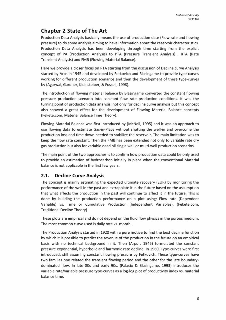
The decline curve analysis theory starts with the concept of the nominal decline rate (D).

Nominal Decline (D) is defined as the fractional change in rate per unit time which is the

negative slope of natural logarithm of the production rate Q vs. time t as shown in

Equation 2-1

𝐷 = −𝑑𝑙𝑛(𝑞)

𝑑𝑡= −

𝑑𝑞/𝑑𝑡

𝑞 Equation 2-1

Another way of representing the decline rate is based on rate (q) and the decline exponent

constant n.

𝐷 = 𝐾𝑞𝑛 Equation 2-2

Production data could follow different behaviors depending on the attitude the nominal

decline with rate. These behaviors are characterized by the decline exponent constant (n).

Exponential — n = 0

Hyperbolic — n is a value between 0 and 1

Harmonic — n = 1

Figure 1: Nominal Decline at a point in time

Mohamed Amr Aly

S236320

5

Arps’ typecurve analysis was basically used for boundary dominated flow with fairly

constant bottom hole flowing pressure. We first define the n power, initial nominal decline

rate, abandonment time ta and then the ultimate recovery Npa.

Fetkovich typecurve Analysis Theory

(Fetkovich, 1980) explained that Arps are not valid for early time production data (Transient)

and therefore he used the analytical equation for the transient flow to generate type-curves

for transient flow that are combined with the type-curves of the Arps. Using the concepts of

well testing with the empirical equations Arps used in his type-curves.

He used in his study a model of well centered producing well in a circular reservoir with

constant flowing bottom-hole pressure with the same standard assumptions used in

describing the reservoir in well testing. (Fekete.com, Fetkovich Theory)

He used the (Van Everdingen & Hurst, 1949) solution to solve the problem in developing the

equation for the transient period and proving that boundary dominated flow period solution

described by Arps had a theoretical background.

He defined a new term of dimensionless rate and dimensionless time by which he succeeded

to make the new type-curves that has two parts.

𝑞𝐷𝑑 = 𝑞𝐷 [ln (𝑟𝑒𝑟𝑤𝑎

) −1

2] Equation 2-3

𝑡𝐷𝑑 =

𝑡𝐷12 [ln (

𝑟𝑒𝑟𝑤𝑎

)2−12] [ln (

𝑟𝑒𝑟𝑤𝑎

) −12]

Equation 2-4

The left part of Fetkovich type-curves describes the transient dominated flow. This part is

different from qD vs tD type-curves where transient flow was represented only with one cure.

Instead, in Fetkovich type-curves the transient flow was represented by a stem of curves

representing the different reservoir sizes re/rw. From this part we can define the reservoir

characteristics (Permeability, skin and well effective radius rwa). (Fetkovich, 1980)

The right part of Fetkovich type-curves describes the boundary dominated flow in which

Fetkovich succeeded to combine his solution with Arps empirical equation using the new

dimensionless rate and dimensionless time he defined and showed that depending less on

the reservoir size, dimensionless rate is exponentially depending on dimensionless time.

𝑞𝐷𝑑 = 𝑒−𝑡𝐷𝑑

This is exactly the same exponential equation of Arps for exponential decline regime where

b=0. Then he extended this solution to cover the hyperbolic decline and include all possible

decline types that could happen in the boundary dominated flow.

A match will decide the type of decline defined here by (b) which is equal to (n) in Arps

decline curves. In addition, the match will provide with the values of re (Drainage radius), kh,

Di and qi and therefore the reservoir pore volume can be calculated. With knowledge of PVT

and reservoir characteristics we could define the Initial hydrocarbon in place.

Mohamed Amr Aly

S236320

6

Blasingame Typecurve Analysis Theory

(Fekete.com, Blasingame Theory) The previous techniques introduced by Arps and Fetkovich

do not account for variations in bottom-hole flowing pressure and also the change in the

PVT properties of gas with the change of pressure caused by production (Depletion).

(Fetkovich, 1980) believed that the exponent "b" could vary between 0 and 1 and that can

be correlated with fluid properties and recovery mechanism. As a proof; single phase oil flow

would align the exponential decline curve where b=0 (Exponential). However, Single phase

gas flow would exhibit b>0 because of the change in gas properties with production.

(Palacio & Blasingame, 1993) used the concept introduced by Fraim and Wattenbarger of

pseudo time that accounts for the change of gas fluid properties. Therefore, boundary

dominated gas flow against a constant back pressure would exhibit the same behavior that

an oil reservoir would (Exponential Decline b=0).

(Palacio & Blasingame, 1993) introduced a function that would change the variable-

pressure/variable-rates solution into an equivalent constant pressure or constant rate

solutions. They reported that using a pressure-normalized flow rate when the bottom hole

pressure varied significantly is not a remedy of the problem, refereeing to variable

rate/variable pressure situation. They introduced two time functions, tcr the constant rate

time function and tcp for constant pressure. Plotting the pressure normalized rate vs. tcr on a

log-log scale will result in a negative unit slope line for boundary dominated flow.

Later, (Palacio & Blasingame, 1993) introduced a superposition time function that accounts

for the variable rate/variable pressure production conditions to appear as constant rate

production regime and what used to match the exponential decline on Fetkovich would

match the harmonic decline on Blasingame type-curves. This time function is called Material

Balance time.

Using Material Balance time by Blasingame allowed depletion at a constant pressure to

appear as it was depletion at constant flow rate. In fact, (Palacio & Blasingame, 1993) have

shown that boundary dominated flow with both declining pressure and rates appear as

pseudo-steady state depletion at a constant rate provided that the pressure and rate decline

monotonically. This would follow the harmonic decline instead of exponential and

hyperbolic decline curves.

The significance was readily evident by considering the inverse of the flowing pressure

plotted against time, pseudo-steady state depletion at constant flow rate follows a harmonic

decline trend.

(Fekete.com, Blasingame Theory) Blasingame, McCary and Placio developed type-curves

which follow the analytical transient stems as Fetkovich type-curves but with harmonic

decline stem. In addition to overcome the noise of production data and smoothen it to

match the type-curves, they introduced other two functions: Rate Integral and Rate Integral

Derivative.

Mohamed Amr Aly

S236320

7

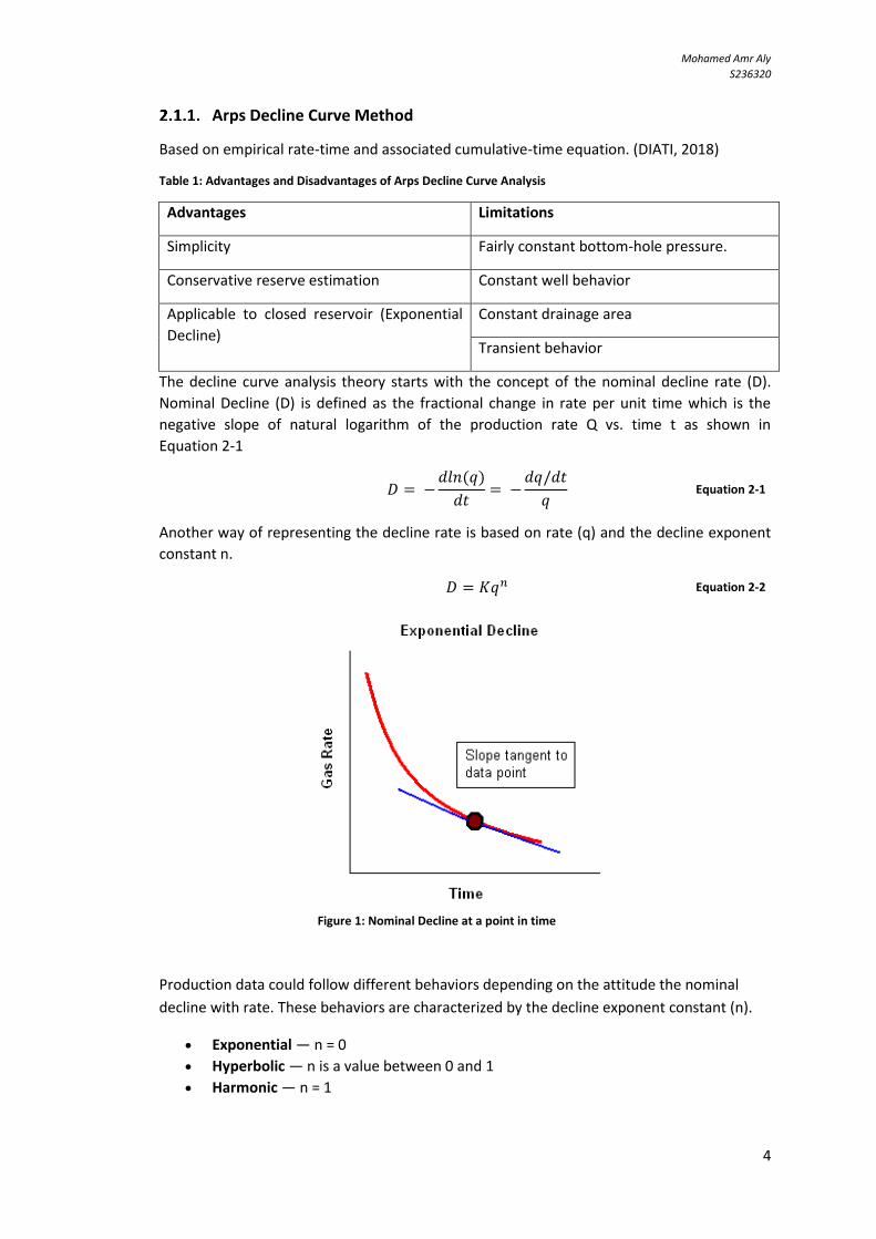
Material Balance Time Theory

(Fekete.com) defined the material balance time as the time needed to produce this

cumulative production amount with the instantaneous flow rate value. Figure 2 shows how

variable rate/variable pressure production scenarios can be transformed into a constant rate

production scenario. (Fekete.com, Material Balance Time Theory)

Material Balance time for Oil:

𝑡𝑐 =𝑁𝑝

𝑞𝑜 Equation 2-5

Material Balance for Gas:

𝑡𝑐𝑔 =𝐺𝑝𝑞𝑔

Equation 2-6

The introduction of material balance time to gas production is different because of the

effect of gas properties change with production. Hence, the concept of oil material balance

time is limitedly used to gas production scenarios. The precise formulation of gas material

balance time is defined as material balance pseudo time (Fekete.com, Material Balance Time

Theory):

𝑡𝑐𝑎 = (𝜇𝑔𝑐𝑔)𝑖𝑞𝑔

∫𝑞𝑔

𝜇𝑔𝑐𝑔̅̅ ̅̅ ̅̅

𝑡

0

𝑑𝑡 Equation 2-7

Figure 2: How material balance time is used to change the variable rate

scenario into constant rate scenario (Fekete.com, Material Balance Time

Theory)

Mohamed Amr Aly

S236320

8

Which in some cases is defined in terms of total compressibility to account for other fluids

compressibilities and the compressibility of rocks:

𝑡𝑐𝑎 = (𝜇𝑔𝑐𝑡)𝑖𝑞𝑔

∫𝑞𝑔

𝜇𝑔𝑐𝑡̅̅ ̅̅ ̅̅

𝑡

0


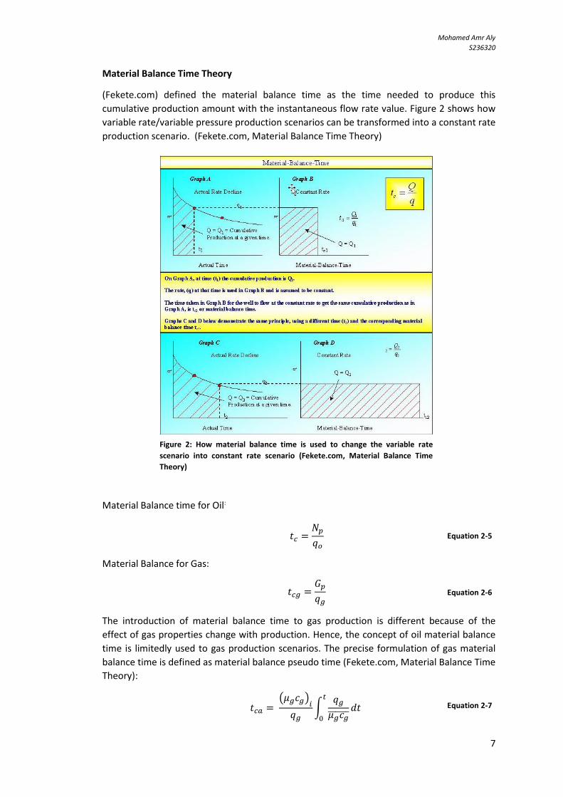
Agarwal Type-curves Theory Analysis

(Agarwal, Gardner, Kleinsteiber, & Fussell, 1998) used the concept developed by Fetkovich,

Palacio and Blasingame of equalizing the constant rate and constant pressure solutions to

introduce the decline type-curves to analyze production data. The dimensionless variables

used by Agarwal and Gardner were built on the conventional well testing definition instead

the ones Fetkovich presented and used by Blasingame. (Fekete.com, Agarwal-Gardner

Theory)

In addition, they included derivative plots (Primary derivative and inverse semi log

derivative) used to illustrate some features between transient and PSS flow in decline

analysis. Moreover, they presented their decline type-curves in additional formats: the rate

vs. cumulative, and cumulative vs. time analysis type-curves. (Fekete.com, Agarwal-Gardner

Theory)

Dimensionless variables used by Agarwal: The dimensionless variables used in type-curves

for pressure transient analysis are dimensionless pressure PwD and its derivative with respect

to dimensionless time 𝑑𝑃𝑤𝐷

𝑑𝑡𝐷 and with respect to log of dimensionless time

𝑑𝑃𝑤𝐷

𝑑𝑙𝑛𝑡𝐷 . To make a

type-curve appear like a decline curve we should use the reciprocal of PwD to produce a

graph of 1

𝑃𝑤𝐷 and

1

𝑑𝑃𝑤𝐷

𝑑𝑙𝑛𝑡𝐷 plotted against dimensionless time. (Agarwal, Gardner, Kleinsteiber,

& Fussell, 1998)

Production Decline Type-curves are represented in three types:

Rate – Time

Rate – Cumulative production

Cumulative production – time.

Mohamed Amr Aly

S236320

9

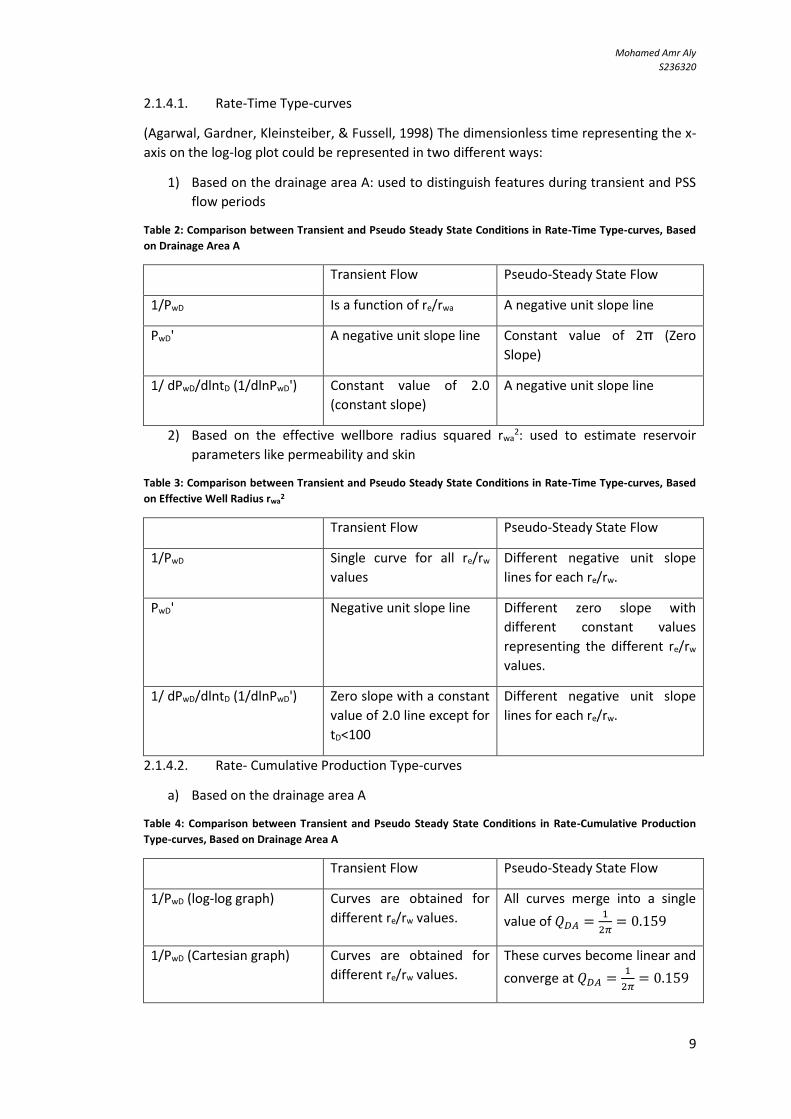
2.1.4.1. Rate-Time Type-curves

(Agarwal, Gardner, Kleinsteiber, & Fussell, 1998) The dimensionless time representing the x-

axis on the log-log plot could be represented in two different ways:

1) Based on the drainage area A: used to distinguish features during transient and PSS

flow periods

Table 2: Comparison between Transient and Pseudo Steady State Conditions in Rate-Time Type-curves, Based

on Drainage Area A

Transient Flow Pseudo-Steady State Flow

1/PwD Is a function of re/rwa A negative unit slope line

PwD' A negative unit slope line Constant value of 2π (Zero

Slope)

1/ dPwD/dlntD (1/dlnPwD') Constant value of 2.0

(constant slope)

A negative unit slope line

2) Based on the effective wellbore radius squared rwa2: used to estimate reservoir

parameters like permeability and skin

Table 3: Comparison between Transient and Pseudo Steady State Conditions in Rate-Time Type-curves, Based

on Effective Well Radius rwa2


1/PwD Single curve for all re/rw

values

Different negative unit slope

lines for each re/rw.

PwD' Negative unit slope line Different zero slope with

different constant values

representing the different re/rw

values.

1/ dPwD/dlntD (1/dlnPwD') Zero slope with a constant

value of 2.0 line except for

tD<100

Different negative unit slope

lines for each re/rw.

2.1.4.2. Rate- Cumulative Production Type-curves

a) Based on the drainage area A

Table 4: Comparison between Transient and Pseudo Steady State Conditions in Rate-Cumulative Production

Type-curves, Based on Drainage Area A


1/PwD (log-log graph) Curves are obtained for

different re/rw values.

All curves merge into a single

value of 𝑄𝐷𝐴 =1

2𝜋= 0.159

1/PwD (Cartesian graph) Curves are obtained for

different re/rw values.

These curves become linear and

converge at 𝑄𝐷𝐴 =1

2𝜋= 0.159

Mohamed Amr Aly

S236320

11

(Agarwal, Gardner, Kleinsteiber, & Fussell, 1998) The significance of that feature that an

approximate estimation of the Initial Hydrocarbon in Place would fit the production data at

the anchor point 𝑄𝐷𝐴 =1

2𝜋= 0.159. Optimistic estimation would undershoot the anchor

point and a pessimistic estimate will overshoot the anchor point.

b) Based on the effective wellbore radius squared rwa2

Table 5: Comparison between Transient and Pseudo Steady State Conditions in Rate-Cumulative Production

Type-curves, Based on Effective Well Radius rwa2


1/PwD One curve with a negative

slope for all re/rwa values

Different seemingly vertical

lines for different values of

re/rwa

PwD' One negative unit slope

curve

Positive different positive unit

slope curves for different values

of re/rwa

(Agarwal, Gardner, Kleinsteiber, & Fussell, 1998) The feature of this graph is that 1/PwD and

the derivative forms an envelope with a vertical tangent corresponding to the Initial

Hydrocarbon in Place.

2.1.4.3. Cumulative Production- Time Type-curves

Based on the effective wellbore radius squared rwa2

Table 6: Comparison between Transient and Pseudo Steady State Conditions in Cumulative Production-Time

Type-curves, Based on Effective Well Radius rwa2


QaD Vs. tD (Log-Lg graph) Single Curve is obtained

for all re/rwa values with a

unit slope except for

tD<100

The curves stabilize and

become flat at different times

according to the value of re/rwa

(Agarwal, Gardner, Kleinsteiber, & Fussell, 1998) These type-curves allow us to use

production data with the absence of transient data and would be a useful tool to

characterize some reservoir parameters (Permeability, skin and reserves).

2.2. Flowing Material Balance When Flowing Material was first introduced for gas production in pseudo steady state

conditions where the pressure decline at any point in the reservoir at the same rate and

therefore, ∆𝑝𝑤𝑓 = ∆𝑝𝑎𝑣𝑔 and then by plotting 𝑃𝑤𝑓

𝑍 vs 𝐺𝑝 we will get a line. Knowing Pi we

can draw a line from 𝑃𝑖

𝑍 parallel to

𝑃𝑤𝑓

𝑍 that intersect the x-axis in G. This was the main

concept introduced by (McNeil, 1995) as the Flowing Material Concept.

This approach was verified in some case studies, and the results of Initial Gas in Place were

not far from the values obtained by conventional Material Balance or numerical simulation

models. (Fekete.com, Flowing Material Balance Theory)

Mohamed Amr Aly

S236320

11

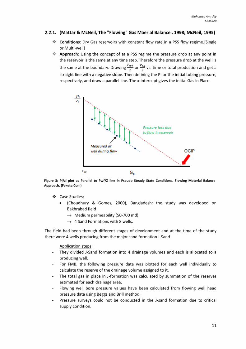
(Mattar & McNeil, The "Flowing" Gas Maerial Balance , 1998; McNeil, 1995)

Conditions: Dry Gas reservoirs with constant flow rate in a PSS flow regime.[Single

or Multi-well]

Approach: Using the concept of at a PSS regime the pressure drop at any point in

the reservoir is the same at any time step. Therefore the pressure drop at the well is

the same at the boundary. Drawing 𝑃𝑤𝑓

𝑍 or

𝑃𝑡ℎ

𝑍 vs. time or total production and get a

straight line with a negative slope. Then defining the Pi or the initial tubing pressure,

respectively, and draw a parallel line. The x-intercept gives the initial Gas in Place.

Case Studies:

(Choudhury & Gomes, 2000), Bangladesh: the study was developed on

Bakhrabad field

Medium permeability (50-700 md)

4 Sand Formations with 8 wells.

The field had been through different stages of development and at the time of the study

there were 4 wells producing from the major sand formation J-Sand.

Application steps:

- They divided J-Sand formation into 4 drainage volumes and each is allocated to a

producing well.

- For FMB, the following pressure data was plotted for each well individually to

calculate the reserve of the drainage volume assigned to it.

- The total gas in place in J-formation was calculated by summation of the reserves

estimated for each drainage area.

- Flowing well bore pressure values have been calculated from flowing well head

pressure data using Beggs and Brill method.

- Pressure surveys could not be conducted in the J-sand formation due to critical

supply condition.

Figure 3: Pi/zi plot as Parallel to Pwf/Z line in Pseudo Steady State Conditions. Flowing Material Balance

Approach. (Fekete.Com)

Mohamed Amr Aly

S236320

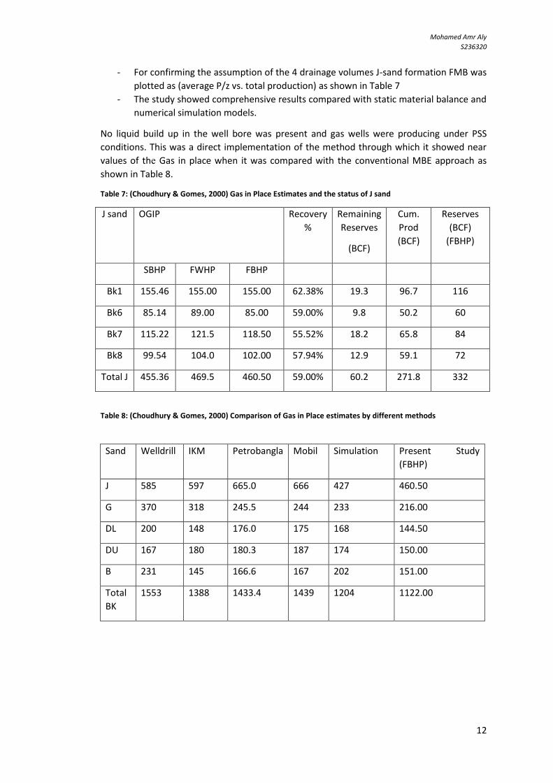
12

- For confirming the assumption of the 4 drainage volumes J-sand formation FMB was

plotted as (average P/z vs. total production) as shown in Table 7

- The study showed comprehensive results compared with static material balance and

numerical simulation models.

No liquid build up in the well bore was present and gas wells were producing under PSS

conditions. This was a direct implementation of the method through which it showed near

values of the Gas in place when it was compared with the conventional MBE approach as

shown in Table 8.

Table 7: (Choudhury & Gomes, 2000) Gas in Place Estimates and the status of J sand

J sand OGIP Recovery

% Remaining

Reserves

(BCF)

Cum.

Prod

(BCF)

Reserves

(BCF)

(FBHP)

SBHP FWHP FBHP

Bk1 155.46 155.00 155.00 62.38% 19.3 96.7 116

Bk6 85.14 89.00 85.00 59.00% 9.8 50.2 60

Bk7 115.22 121.5 118.50 55.52% 18.2 65.8 84

Bk8 99.54 104.0 102.00 57.94% 12.9 59.1 72

Total J 455.36 469.5 460.50 59.00% 60.2 271.8 332

Table 8: (Choudhury & Gomes, 2000) Comparison of Gas in Place estimates by different methods

Sand Welldrill IKM Petrobangla Mobil Simulation Present Study

(FBHP)

J 585 597 665.0 666 427 460.50

G 370 318 245.5 244 233 216.00

DL 200 148 176.0 175 168 144.50

DU 167 180 180.3 187 174 150.00

B 231 145 166.6 167 202 151.00

Total

BK

1553 1388 1433.4 1439 1204 1122.00

Mohamed Amr Aly

S236320

13

(Guzman, Arevalo, & Espinola, 2014) provided a case study of implementing

FMB for estimating on two Dry Gas reservoirs in Mexico.

A (22 producing well, 4 with downhole sensors).

B (7 producing wells, 2 with downhole sensors).

For some wells it was possible to have information about static and dynamic pressure

profiles.

Table 9: (Guzman, Arevalo, & Espinola, 2014) Summary of OGIP (MMSCF) Calculation by Different Studies

Study

Volumetric

Decline

Curve

Analysis

Conventional

Material

Balance

Reservoir

Numerical

Simulation

Flowing

Gas

Maerial

Balance

Difference

FDMB vs

Numerical

Simulation

Reservoir

1 Field A

552 424.6 701 510 499 2.2%

Reservoir

1 Field B

97 69 81 86 93 8%

However, for the ones that lack information, data was modeled through tubing head

pressure and a multiphase flow simulator.

The large difference between conventional and flowing material balance for field A in Table

9 was due to the lack of shut-in pressure.

Results in Figure 9 showed error that did not exceed 10% that could be acceptable in case of

the need of estimating the initial Gas in place with no shut-in pressure.

(Mattar & Anderson, Dynamic Material Balance(Oil or Gas-In-Place Without

Shut-In), 2005)

Conditions: For under saturated oil reservoir and Dry Gas reservoir both constant or

variable flow rate scenarios. Boundary Dominated flow should be existing.

Approach: this method uses the flowing data at any point to convert the measure

flowing pressure to the average pressure that exists at the reservoir at this time.

Then, using the calculated average pressure and the corresponding cumulative

production we can calculate the original volume in place by the conventional

material balance method.

a) FMB [Constant Rate, Gas]: The use of the previously explained method of

(McNeil, 1995) and (Mattar & McNeil, 1998)

b) FMB [Constant rate, Oil]: Using the Pseudo Steady State equation with the

depletion equation of under-saturated oil reservoir we reach this equation:

𝑃𝑖 − 𝑃𝑤𝑓 =𝑞𝑜𝑡

𝐶𝑜𝑁+ 141.2 𝑞𝑜𝐵𝑜𝜇𝑜

𝑘ℎ[ln (

𝑟𝑒𝑟𝑤) −

3

4] Equation 2-9

This can be written as: 𝑃𝑖 − 𝑃𝑤𝑓 =𝑞𝑜𝑡

𝐶𝑜𝑁+ 𝑏𝑝𝑠𝑠 𝑞𝑜 Equation 2-10

Mohamed Amr Aly

S236320

14

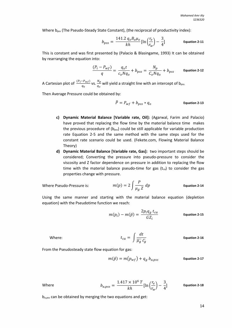
Where bpss (The Pseudo-Steady State Constant), (the reciprocal of productivity index):

𝑏𝑝𝑠𝑠 = 141.2 𝑞𝑜𝐵𝑜𝜇𝑜

𝑘ℎ[ln (


3

4] Equation 2-11

This is constant and was first presented by (Palacio & Blasingame, 1993) It can be obtained

by rearranging the equation into:

(𝑃𝑖 − 𝑃𝑤𝑓)

𝑞=

𝑞𝑜𝑡

𝑐𝑜𝑁𝑞𝑜+ 𝑏𝑝𝑠𝑠 =

𝑁𝑝𝐶𝑜𝑁𝑞o

+ 𝑏𝑝𝑠𝑠 Equation 2-12

A Cartesian plot of (𝑃𝑖−𝑃𝑤𝑓)

𝑞0 vs.

𝑁𝑝

𝑞𝑜 will yield a straight line with an intercept of bpss.

Then Average Pressure could be obtained by:

�̅� = 𝑃𝑤𝑓 + 𝑏𝑝𝑠𝑠 ∗ 𝑞𝑜 Equation 2-13

c) Dynamic Material Balance [Variable rate, Oil]: (Agarwal, Farim and Palacio)

have proved that replacing the flow time by the material balance time makes

the previous procedure of (bpss) could be still applicable for variable production

rate Equation 2-5 and the same method with the same steps used for the

constant rate scenario could be used. (Fekete.com, Flowing Material Balance

Theory)

d) Dynamic Material Balance [Variable rate, Gas]: two important steps should be

considered; Converting the pressure into pseudo-pressure to consider the

viscosity and Z factor dependence on pressure in addition to replacing the flow

time with the material balance pseudo-time for gas (tca) to consider the gas

properties change with pressure.

Where Pseudo-Pressure is: 𝑚(𝑝) = 2∫𝑃

𝜇𝑔 𝑍 𝑑𝑝 Equation 2-14

Using the same manner and starting with the material balance equation (depletion

equation) with the Pseudotime function we reach:

𝑚(𝑝𝑖) − 𝑚(�̅�) = 2𝑝𝑖𝑞𝑔 𝑡𝑐𝑎

𝐺𝑍𝑖 Equation 2-15

Where: 𝑡𝑐𝑎 = ∫𝑑𝑡

𝜇𝑔̅̅ ̅ 𝑐�̅� Equation 2-16

From the Pseudosteady state flow equation for gas:

𝑚(�̅�) = 𝑚(𝑝𝑤𝑓) + 𝑞𝑔 𝑏𝑎,𝑝𝑠𝑠 Equation 2-17

Where 𝑏𝑎,𝑝𝑠𝑠 = 1.417 × 106 𝑇

𝑘ℎ[ln (


3

4] Equation 2-18

ba,pss can be obtained by merging the two equations and get:

Mohamed Amr Aly

S236320

15

∆𝑚(𝑝) =24 ∗ 2348 ∗ 𝑇 𝑞𝑔 𝑡𝑐𝑎

𝜋 𝜙 𝜇𝑔𝑖 𝑐𝑔𝑖 𝑟𝑒2 ℎ

+1.417 ∗ 106 𝑇 𝑞

𝑘ℎ[ln (


3

4]

Equation 2-19

Then average pseudo pressure can be calculated through Equation 2-17 that would be

converted to average pressure to plot the gas P/z plot vs Gp

(Mattar & Anderson, 2005)) provided the steps of the "Dynamic Material Balance" for gas

production a variable flow rate are:

1. Convert initial pressure and the flowing pressures to pseudo pressures, 𝑚(𝑝𝑖),

𝑚(𝑝𝑤𝑓)

2. Assume an initial value for G to calculate the average reservoir pressure values

corresponding to the cumulative production.

3. Calculate Pseudotime function tca based on the gas properties estimated at the

average pressure values.

4. Plot ∆𝑚(𝑝)

𝑞𝑔 vs. pseudo material balance time 𝑡𝑐𝑎 and the intercept gives ba,pss.

5. Calculate the average pseudo-pressure

6. Convert the average pseudo-pressure to average reservoir pressure

7. Calculate P/z values and plot them against Gp just like conventional MBE and get

the intercept, G

8. Iterate until reaching a good convergence for the G value.

**Note: When Equation 2-15 was compared with other literature it showed that the

dominator misses the gas viscosity and compressibility

𝑚(𝑝𝑖) − 𝑚(�̅�) =2𝑝𝑖𝑞 𝑡𝑐𝑎𝐺𝑍𝑖

Equation 2-20

In our thesis work we will call the Dynamic Material Balance for a variable gas rate

production as the Gas Flowing Material Balance Approach to generalize the concept

and to be easier compared with the other approaches implemented.

Mohamed Amr Aly

S236320

16

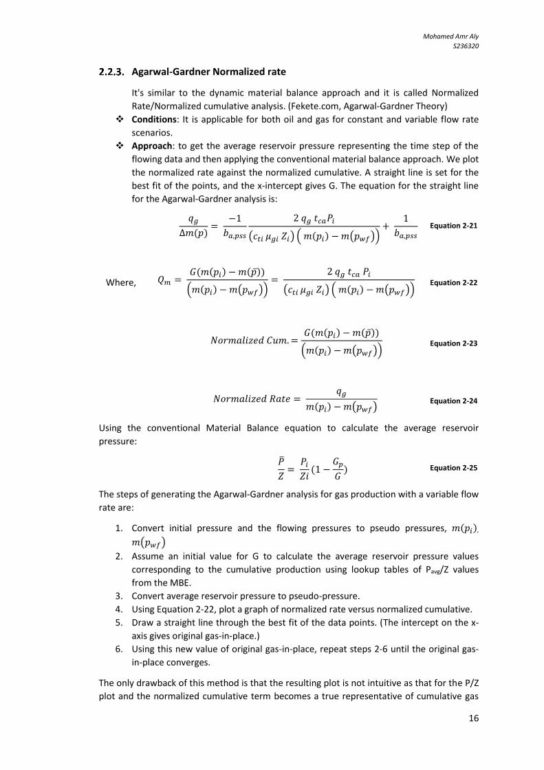
Agarwal-Gardner Normalized rate

It's similar to the dynamic material balance approach and it is called Normalized

Rate/Normalized cumulative analysis. (Fekete.com, Agarwal-Gardner Theory)

Conditions: It is applicable for both oil and gas for constant and variable flow rate

scenarios.

Approach: to get the average reservoir pressure representing the time step of the

flowing data and then applying the conventional material balance approach. We plot

the normalized rate against the normalized cumulative. A straight line is set for the

best fit of the points, and the x-intercept gives G. The equation for the straight line

for the Agarwal-Gardner analysis is:

𝑞𝑔

∆𝑚(𝑝)=

−1

𝑏𝑎,𝑝𝑠𝑠

2 𝑞𝑔 𝑡𝑐𝑎𝑃𝑖

(𝑐𝑡𝑖 𝜇𝑔𝑖 𝑍𝑖) ( 𝑚(𝑝𝑖) −𝑚(𝑝𝑤𝑓))+

1

𝑏𝑎,𝑝𝑠𝑠 Equation 2-21

Where, 𝑄𝑚 = 𝐺(𝑚(𝑝𝑖) − 𝑚(�̅�))

(𝑚(𝑝𝑖) − 𝑚(𝑝𝑤𝑓))=

2 𝑞𝑔 𝑡𝑐𝑎 𝑃𝑖

(𝑐𝑡𝑖 𝜇𝑔𝑖 𝑍𝑖) ( 𝑚(𝑝𝑖) −𝑚(𝑝𝑤𝑓)) Equation 2-22

𝑁𝑜𝑟𝑚𝑎𝑙𝑖𝑧𝑒𝑑 𝐶𝑢𝑚.=𝐺(𝑚(𝑝𝑖) − 𝑚(�̅�))

(𝑚(𝑝𝑖) − 𝑚(𝑝𝑤𝑓)) Equation 2-23

𝑁𝑜𝑟𝑚𝑎𝑙𝑖𝑧𝑒𝑑 𝑅𝑎𝑡𝑒 = 𝑞𝑔

𝑚(𝑝𝑖) − 𝑚(𝑝𝑤𝑓) Equation 2-24

Using the conventional Material Balance equation to calculate the average reservoir

pressure:

�̅�

𝑍= 𝑃𝑖𝑍𝑖(1 −

𝐺𝑝𝐺) Equation 2-25

The steps of generating the Agarwal-Gardner analysis for gas production with a variable flow

rate are:

1. Convert initial pressure and the flowing pressures to pseudo pressures, 𝑚(𝑝𝑖),

𝑚(𝑝𝑤𝑓)

2. Assume an initial value for G to calculate the average reservoir pressure values

corresponding to the cumulative production using lookup tables of Pavg/Z values

from the MBE.

3. Convert average reservoir pressure to pseudo-pressure.

4. Using Equation 2-22, plot a graph of normalized rate versus normalized cumulative.

5. Draw a straight line through the best fit of the data points. (The intercept on the x-

axis gives original gas-in-place.)

6. Using this new value of original gas-in-place, repeat steps 2-6 until the original gas-

in-place converges.

The only drawback of this method is that the resulting plot is not intuitive as that for the P/Z

plot and the normalized cumulative term becomes a true representative of cumulative gas

Mohamed Amr Aly

S236320

17

production only when the material balance line intercept the cumulative gas production line

and nowhere else.

Case Study: (Ismadi, Kabir, & Hasan, 2012) provided a case study that compares the

two approaches (Dynamic Material Balance of Gas by (Mattar & Anderson, 2005)

and Agarwal – Gardner Analysis in estimating the original gas initially in place. The

difference between the two methods was in calculating the average reservoir

pressure by which the conventional material balance is applied. The DMB by (Mattar

& Anderson, 2005) showed more iterative steps and values of Initial Gas in place

were not similar to the ones calculated by the actual static pressure data with

conventional MBE as shown in Figure 4: (Ismadi, Kabir, & Hasan, 2012) Comparison

of the two FMB approaches [Gas FMB vs. Agarwal] for homogenous system. The

reason is that any variations happen in the flowing data is reflected in ba,pss and then

in calculating the average reservoir pressure. However, Agarwal's method includes a

combined approach of static material balance with his normalized rate/normalized

cumulative in calculating average reservoir pressure and then G.

Figure 4: (Ismadi, Kabir, & Hasan, 2012) Comparison of the two FMB approaches [Gas FMB vs. Agarwal] for

homogenous system.

Mohamed Amr Aly

S236320

18

Flowing Material Balance using a new Pseudotime function

This approach was presented by (Mohammed & Enty, 2013) in their paper of Analysis of Gas

Production Using Flowing Material Balance Method where:

- Provided a derivation for a new pseudotime material balance function through which he

proved the theoretical background of the material balance time and it is not just intuitive as

it has been considered for years.

- They also provided a flow equation based on this new pseudotime function that represents

the flow rate normalized pseudo cumulative that has been first introduced by (Callard &

Schenewerk, 1995), but not used for this approach.

- Provided a simpler approach to calculate Gas-In-Place after defining PSS regime using type-

curves.

- Provided a method to validate computed initial gas in place calculated by any method.

Between The Material Pseudotime and The new Pseudotime Functions

Material Balance Pseudotime (tca) has gained a widespread acceptance as it has the ability

to handle the variable pressure or variable rate scenarios and it also considers the variations

of gas properties (Viscosity and compressibility) with the average reservoir pressure change.

Although it’s suitable to handle long term boundary dominated flow and it's rigorous for real

gas, it's dependent on time step size and it's not suitable for shut in periods and requires the

knowledge of average reservoir pressure or indirectly Gas-in-place.

It has first introduced by Palacio and Blasingame (1993) and used by Agarwal (1999) and

Mattar and Anderson (2005) included in the gas flow equations applied for Flowing Material

Balance approaches.

The New Pseudotime Function (Ta) is not sensitive to the time step size and offers a simpler

approach to handle the viscosity-compressibility variations as viscosity-compressibility ratio

is a function of the cumulative production. Viscosity-Compressibility variation showed a

sensitive impact on the flowing material balance field data that have been plotted. It

appeared as a fluctuation in the late-time boundary dominated flow data that caused a

change in the slop of the straight line.

It is defined as: 𝑇𝑎 = 1

𝑞𝑔∫

(𝜇𝑔𝑐𝑡)𝑖𝜇𝑔̅̅ ̅̅ 𝑐�̅�

𝐺𝑝0

𝑑𝐺𝑝 Equation 2-26

(Mohammed & Enty, 2013) provided a simple approach to include the new material balance

pseudo time in the general flow equation for variable rate or variable pressure scenarios.

They started from the general expression for 𝑑�̅� is given by (Farim and Wattenbarger 1987):

𝑑�̅� = −𝑞𝑔𝐵𝑔

𝑉𝑃𝑆𝑔𝑖𝑐�̅� 𝑑𝑡 Equation 2-27

Where the relation between gas cumulative production and gas flow rate is given by:

𝑞𝑔 = 𝑑𝐺𝑝


Combining Equation 2-27 and Equation 2-28 yields:

Mohamed Amr Aly

S236320

19

𝑑�̅� = −𝐵𝑔

𝑉𝑃𝑆𝑔𝑖𝐶�̅�𝑑𝐺𝑝 Equation 2-29

Knowing that formation volume factor can be expressed as:

𝐵𝑔 = �̅�𝑇 𝑃𝑠𝑐

�̅�𝑇𝑠𝑐 Equation 2-30

Therefore, by substitution in Equation 2-29 we have:

𝑑�̅� = − �̅�𝑇

𝑃(𝑃𝑠𝑐𝑇𝑠𝑐) [

1

𝑉𝑃𝑆𝑔𝑖𝐶�̅�] 𝑑𝐺𝑃 Equation 2-31

Here, we introduce the normalized pseudopressure given by (Meunier, Kabir, & Wittmann,

1987) and (Palacio & Blasingame, 1993):

𝑚(�̅�)𝑛 =(𝜇𝑔𝑍)𝑖𝑃𝑖

∫�̅�

�̅��̅�𝑑�̅�

𝑃

0

Equation 2-32

This is differentiated to give:

𝑑𝑚(�̅�)𝑛 =(𝜇𝑔𝑍)𝑖𝑃𝑖

�̅�

�̅��̅�𝑑�̅� Equation 2-33

Now we substitute Equation 2-31 into Equation 2-33 and we get:

−𝑑𝑚(�̅�)𝑛 = [𝑇

𝑉𝑃𝑆𝑔𝑖 (𝑃𝑖𝑍𝑖⁄ )

(𝑃𝑠𝑐𝑇𝑠𝑐)]

𝜇𝑔𝑖

𝜇𝑔̅̅ ̅𝐶�̅� 𝑑𝐺𝑝 Equation 2-34

Initial Gas in Place is expressed as:

𝐺 = 𝑉𝑃𝑆𝑔𝑖 (

𝑃𝑖𝑍𝑖⁄ )

𝑇 (𝑇𝑠𝑐𝑃𝑠𝑐) Equation 2-35

We combine Equation 2-34 & Equation 2-35to have:

−𝑑𝑚(�̅�)𝑛 = [𝜇𝑔𝑖

𝐺]1

𝜇𝑔̅̅ ̅𝐶�̅� 𝑑𝐺𝑝 Equation 2-36

We can now integrate Equation 2-36 from the initial normalized pseudopressure, which

corresponds to zero cumulative, to any given average reservoir pressure, which corresponds

to a cumulative production of GP. In other words, we are integrating from initial time (i.e.,

t=0) to any given time, t, to reach:

− ∫ 𝑑𝑚(�̅�)𝑛𝑚(�̅�)𝑛𝑚(𝑃𝑖)𝑛

= 1

𝐺𝐶𝑡𝑖∫

(𝜇𝑔𝑖𝐶𝑡𝑖)

𝜇𝑔̅̅ ̅̅ 𝐶𝑡̅̅ ̅ 𝑑𝐺𝑝

𝐺𝑝0

Equation 2-37

Which then becomes: 𝑚(𝑃𝑖)𝑛 − 𝑚(�̅�)𝑛 = 1

𝐺𝐶𝑡𝑖∫


𝜇𝑔̅̅ ̅𝐶�̅� 𝑑𝐺𝑝

𝐺𝑝

0

Equation 2-38

Here, we introduce the pseudocumulative function given by (Callard & Schenewerk, 1995)

Mohamed Amr Aly

S236320

21

𝐺𝑝𝑛 = ∫(𝜇𝑔𝑖𝐶𝑡𝑖)


𝐺𝑝

0

Equation 2-39

Therefore, 𝑚(�̅�)𝑛 = 𝑚(𝑃𝑖)𝑛 − 1

𝐺𝐶𝑡𝑖 𝐺𝑝𝑛 Equation 2-40

This equation is similar now to the liquid material balance given by (Dake):

�̅� = 𝑃𝑖 − 1

𝑁𝐶𝑡𝑁𝑝 Equation 2-41

Using normalized pseudo pressure instead of actual pressure and pseudocumulative instead

of actual cumulative linearizes the single phase gas flow equation and this allows us to solve

single phase problems with the liquid solution.

Including gas flow equation during Pseudosteady state (PSS) flow regime is given by (Palacio

& Blasingame, 1993):

𝑚(�̅�)𝑛 −𝑚(𝑃𝑤𝑓) = 𝑞𝑔𝑏𝑎,𝑝𝑠𝑠 Equation 2-42

Then we combine Equation 2-38 and Equation 2-42 to have:

𝑚(𝑃𝑖)𝑛− 𝑚(𝑃𝑤𝑓)𝑛

𝑞𝑔= [

1

𝐺𝐶𝑡𝑖∫

1

𝑞𝑔


𝜇𝑔̅̅ ̅̅ 𝐶𝑡̅̅ ̅ 𝑑𝐺𝑝

𝐺𝑝0

] + 𝑏𝑎,𝑝𝑠𝑠 Equation 2-43

And the expression in the bracket on the right hand side (RHS) of Equation 2-46 becomes our

basis for defining the new material balance Pseudotime function Ta in Equation 2-26

𝑚(𝑃𝑖)𝑛− 𝑚(𝑃𝑤𝑓)𝑛

𝑞𝑔=

1

𝐺𝐶𝑡𝑖𝑇𝑎 + 𝑏𝑎,𝑝𝑠𝑠 Equation 2-44

Equation 2-44 shows that both the material balance pseudotime function and the new

function have sound theoretical proof and they are equivalent.

𝑚(𝑃𝑖)𝑛 − 𝑚(𝑃𝑤𝑓)𝑛

𝑞𝑔=

1

𝐺𝐶𝑡𝑖

𝐺𝑝𝑛𝑞𝑔

+ 𝑏𝑎,𝑝𝑠𝑠 Equation 2-45

By Plotting Equation 2-45 we get the x-intercept as G*Cti

𝑞𝑔

∆𝑚(𝑝)𝑛= −

1

𝑏𝑎,𝑝𝑠𝑠 𝐺𝐶𝑡𝑖

𝐺𝑝𝑛∆𝑚(𝑝)𝑛

+1

𝑏𝑎,𝑝𝑠𝑠 Equation 2-46

(Mohammed & Enty, 2013) Stated the steps for the FMB approach using the new material

balance pseudo function using the normalized pseudo cumulative function:

1. Make a polynomial plot of viscosity-compressibility ratio against actual cumulative production at least to the third degree and set the intercept to 1. In our study for more accurate we developed it to the fifth order.

2. Integrate the resulting polynomial equation with respect to the actual cumulative production.

3. Substitute each actual cumulative production data point into the integral expression to obtain the corresponding pseudocumulative.

4. Make an approximate plot using Gp instead of Gpn in the previous equation. If data did not follow one straight line and two segments are observed (i.e., early and late time

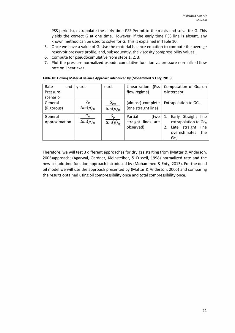
Mohamed Amr Aly

S236320

21

PSS periods), extrapolate the early time PSS Period to the x-axis and solve for G. This yields the correct G at one time. However, if the early time PSS line is absent, any known method can be used to solve for G. This is explained in Table 10.

5. Once we have a value of G. Use the material balance equation to compute the average reservoir pressure profile, and, subsequently, the viscosity compressibility values.

6. Compute for pseudocumulative from steps 1, 2, 3. 7. Plot the pressure normalized pseudo cumulative function vs. pressure normalized flow

rate on linear axes. Table 10: Flowing Material Balance Approach introduced by (Mohammed & Enty, 2013)

Rate and Pressure scenario

y-axis x-axis Linearization (Pss flow regime)

Computation of Gcti on x-intercept

General (Rigorous)

𝑞𝑔

∆𝑚(𝑝)𝑛


(almost) complete (one straight line)

Extrapolation to GCti

General Approximation

𝑞𝑔

∆𝑚(𝑝)𝑛

𝐺𝑝∆𝑚(𝑝)𝑛

Partial (two straight lines are observed)

1. Early Straight line extrapolation to Gcti

2. Late straight line overestimates the Gcti

Therefore, we will test 3 different approaches for dry gas starting from (Mattar & Anderson,

2005)approach; (Agarwal, Gardner, Kleinsteiber, & Fussell, 1998) normalized rate and the

new pseudotime function approach introduced by (Mohammed & Enty, 2013). For the dead

oil model we will use the approach presented by (Mattar & Anderson, 2005) and comparing

the results obtained using oil compressibility once and total compressibility once.

Mohamed Amr Aly

S236320

22

Synthetic Data

[Eclipse]

• Dry Gas: Single Well & Multi Well

• Dead Oil: Single Well & Multi Well

RTA

[Ecrin-Topaze 4.2]

• Model Matching

• Fetkovich & Blasingame Type-curves matching.

FMB

• Dead Oil: Oil compressibility & Total Compressibility

• Dry Gas: Pseudo Material Balance time function, Agarwal - Gardner approach & New Material Balance Function.

Chapter 3 Methodology Studying the two proposed approaches needs to have production data and our study mainly

based on synthetic data developed by Eclipse Simulator. Having the production data enables

us to start analyzing them by Topaze (RTA Interface of Ecrin v4.20.05) by first model

matching and then RTA. The last step is to build Flowing Material Balance approaches to

obtain the Hydrocarbon in place estimation using flowing data.

Figure 5: Steps of Methodology done in this study

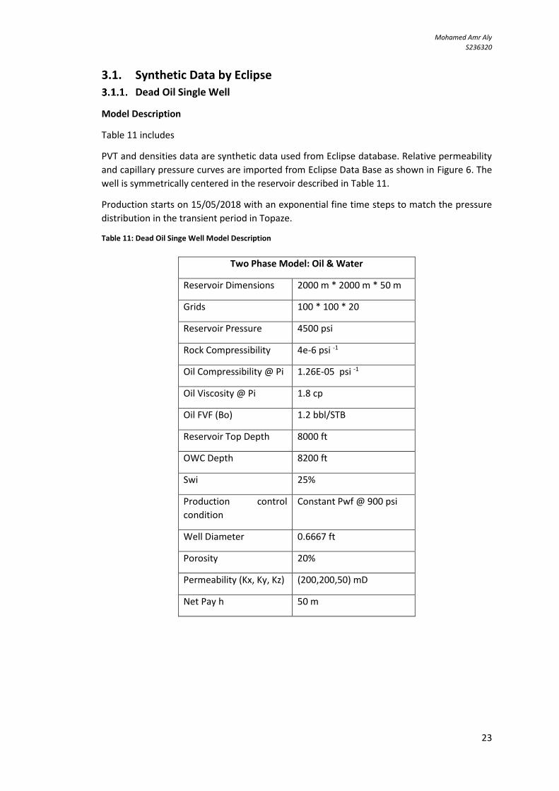
Mohamed Amr Aly

S236320

23

3.1. Synthetic Data by Eclipse


Model Description

Table 11 includes

PVT and densities data are synthetic data used from Eclipse database. Relative permeability

and capillary pressure curves are imported from Eclipse Data Base as shown in Figure 6. The

well is symmetrically centered in the reservoir described in Table 11.

Production starts on 15/05/2018 with an exponential fine time steps to match the pressure

distribution in the transient period in Topaze.

Table 11: Dead Oil Singe Well Model Description

Two Phase Model: Oil & Water

Reservoir Dimensions 2000 m * 2000 m * 50 m

Grids 100 * 100 * 20

Reservoir Pressure 4500 psi

Rock Compressibility 4e-6 psi -1

Oil Compressibility @ Pi 1.26E-05 psi -1

Oil Viscosity @ Pi 1.8 cp

Oil FVF (Bo) 1.2 bbl/STB

Reservoir Top Depth 8000 ft

OWC Depth 8200 ft

Swi 25%

Production control

condition

Constant Pwf @ 900 psi

Well Diameter 0.6667 ft

Porosity 20%

Permeability (Kx, Ky, Kz) (200,200,50) mD

Net Pay h 50 m

Mohamed Amr Aly

S236320

24

Dead Oil Multi Well

For Multi-well we have the same model. The main difference is the number and the location

of the wells. In this model we have 4 wells, symmetrically located. The grid numbers of each

well are shown in Figure 7.

Figure 6: Dead Oil Single Well Eclipse Model PVT data

Figure 7: Dead Oil Single Multi Well Model, Well Locations

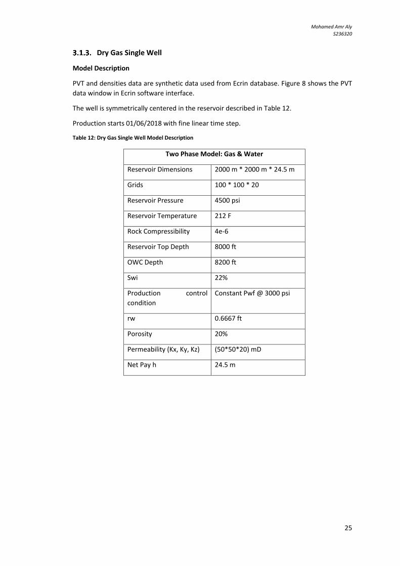
Mohamed Amr Aly

S236320

25

Dry Gas Single Well

Model Description

PVT and densities data are synthetic data used from Ecrin database. Figure 8 shows the PVT

data window in Ecrin software interface.

The well is symmetrically centered in the reservoir described in Table 12.

Production starts 01/06/2018 with fine linear time step.

Table 12: Dry Gas Single Well Model Description

Two Phase Model: Gas & Water

Reservoir Dimensions 2000 m * 2000 m * 24.5 m

Grids 100 * 100 * 20

Reservoir Pressure 4500 psi

Reservoir Temperature 212 F

Rock Compressibility 4e-6

Reservoir Top Depth 8000 ft

OWC Depth 8200 ft

Swi 22%

Production control

condition

Constant Pwf @ 3000 psi

rw 0.6667 ft

Porosity 20%

Permeability (Kx, Ky, Kz) (50*50*20) mD

Net Pay h 24.5 m

Mohamed Amr Aly

S236320

26

Exporting PVT data (Viscosity, Density, Z factor, Gas FVF, Compressibility). As shown in

the figure below, reservoir pressure is set as 4500 psia and reservoir temperature as 212

F. By importing the PVT we could obtain the PVT as a function of pressure at any point.

Therefore we could create PVT table for the Eclipse model from the imported data. Data

imported and used for Eclipse are shown in Figure 9.

Figure 8: Importing PVT data from Ecrin. Topaze database representing our model parameters of Pressure and

temperature

Mohamed Amr Aly

S236320

27

For the relative permeability and capillary pressure curves, data is imported from Eclipse

Database where the SGWFN keyword is used for the two phase model (Water and gas) and

columns represent respectively (Gas saturations, Gas relative permeability values

representing the saturation values, water relative permeability values representing these

saturations and capillary pressure values at these saturations). (Ltd., 2014, p. 2104)

Figure 9: Dry Gas Single Well Eclipse Model PVT data

Figure 10: Dry Gas Single Well Eclipse Model capillary pressure data

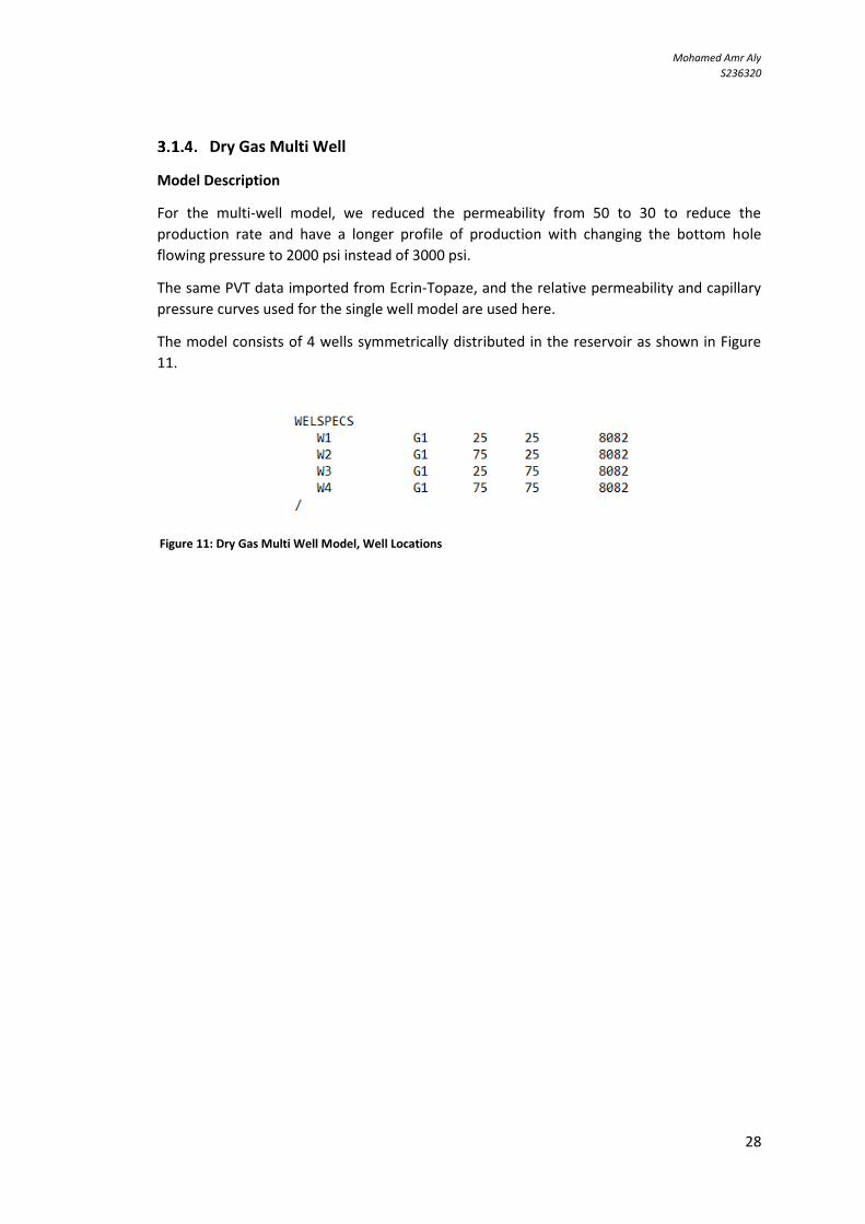
Mohamed Amr Aly

S236320

28

Dry Gas Multi Well

Model Description

For the multi-well model, we reduced the permeability from 50 to 30 to reduce the

production rate and have a longer profile of production with changing the bottom hole

flowing pressure to 2000 psi instead of 3000 psi.

The same PVT data imported from Ecrin-Topaze, and the relative permeability and capillary

pressure curves used for the single well model are used here.

The model consists of 4 wells symmetrically distributed in the reservoir as shown in Figure

11.

Figure 11: Dry Gas Multi Well Model, Well Locations

Mohamed Amr Aly

S236320

29

0

40000

80000

Liquid

rate

[STB

/D]

Prod

uctio

n [ST

B/D]

0 10000 20000 30000 40000 50000 60000 70000Time [hr]

1500

2500

3500

Pres

sure

[psia]

Pres

sure

[psia

]

Liquid rate [STB/D], Pressure [psia] vs Time [hr]

3.2. Rate Transient Analysis [Ecrin v4.20.05- Topaze Interface] After running the model on Eclipse we get the .RSM file with the production data and we

input the production flowing data (Pwf, Qo) in Ecrin for each model. After this we build the

model. For the single well model, we used the analytical approach and for the multi well we

used the numerical model to compare the results of the two approaches.


Figure 13 shows PVT as described in the Eclipse Model. The PVT data are considered

constant for the production profile.

Figure 13: Dead Oil Single Well PVT data input in Ecrin. Topaze

Figure 12: Dead Oil Single Well, Production rate and bottom hole flowing pressure vs. time

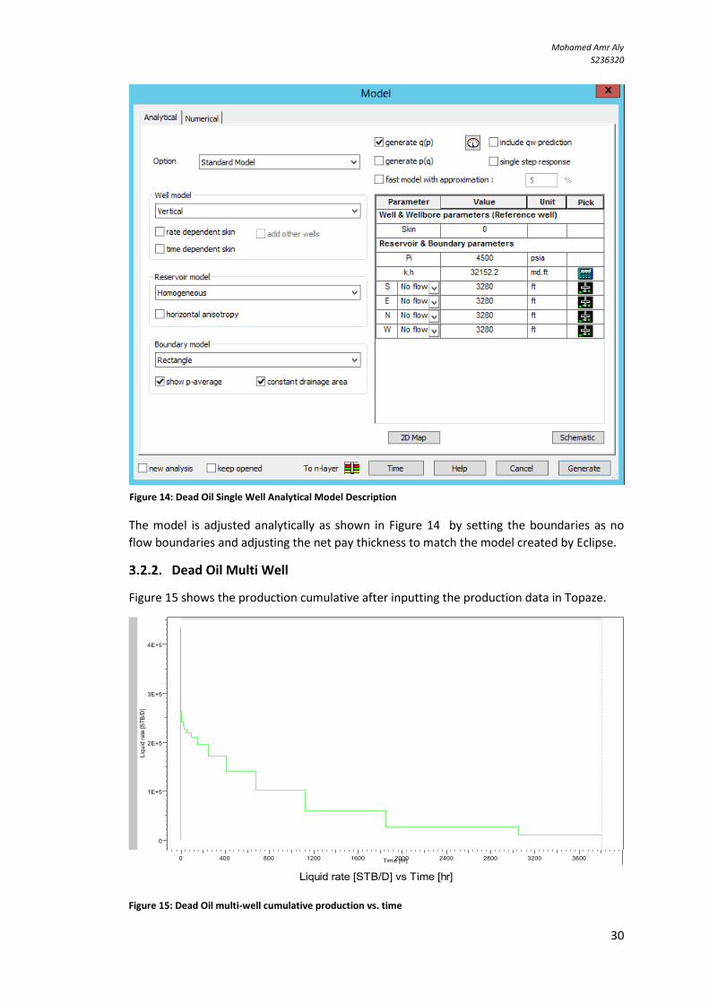
Mohamed Amr Aly

S236320

31

The model is adjusted analytically as shown in Figure 14 by setting the boundaries as no

flow boundaries and adjusting the net pay thickness to match the model created by Eclipse.

Dead Oil Multi Well

Figure 15 shows the production cumulative after inputting the production data in Topaze.

Figure 15: Dead Oil multi-well cumulative production vs. time

0

1E+5

2E+5

3E+5

4E+5

Liqu

id ra

te [S

TB/D

]

Prod

uctio

n [S

TB/D

]

0 400 800 1200 1600 2000 2400 2800 3200 3600Time [hr]

Liquid rate [STB/D] vs Time [hr]

Figure 14: Dead Oil Single Well Analytical Model Description

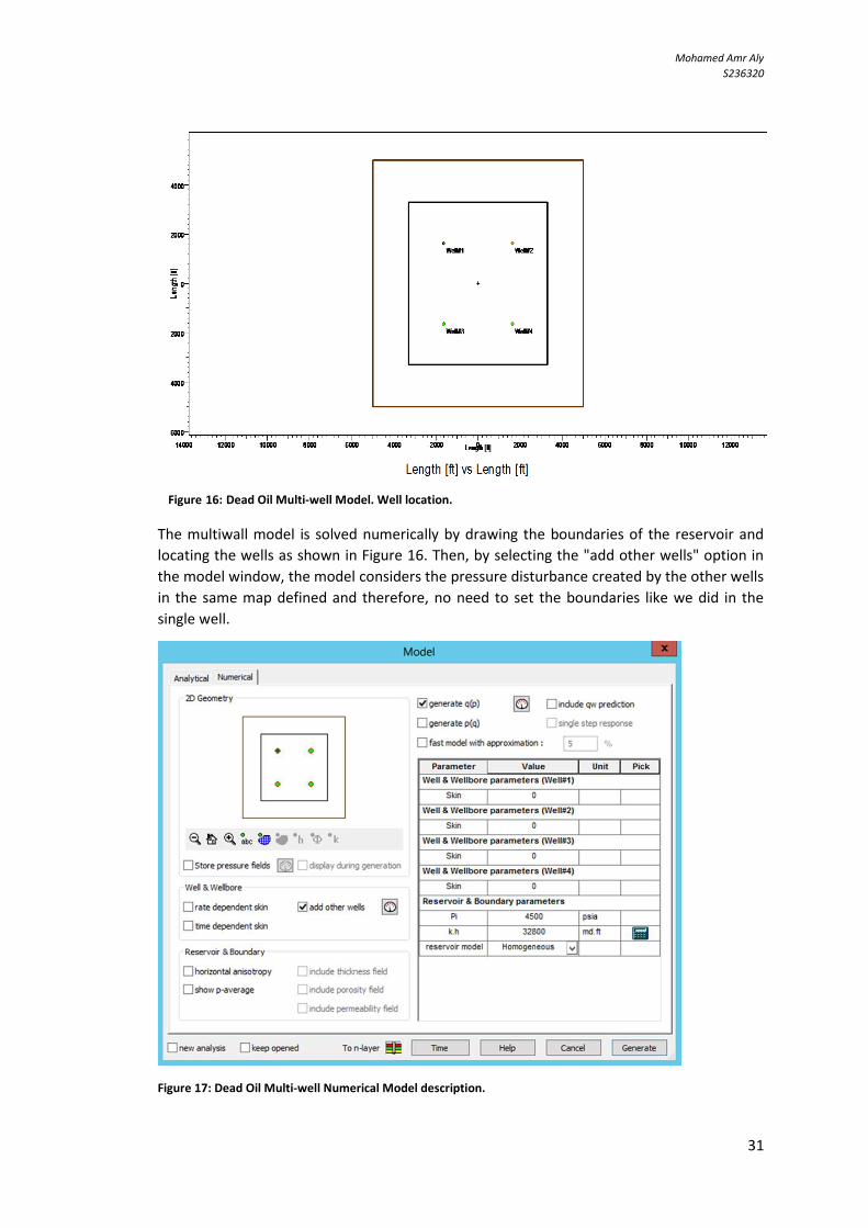
Mohamed Amr Aly

S236320

31

The multiwall model is solved numerically by drawing the boundaries of the reservoir and

locating the wells as shown in Figure 16. Then, by selecting the "add other wells" option in

the model window, the model considers the pressure disturbance created by the other wells

in the same map defined and therefore, no need to set the boundaries like we did in the

single well.

Figure 17: Dead Oil Multi-well Numerical Model description.

Figure 16: Dead Oil Multi-well Model. Well location.

Mohamed Amr Aly

S236320

32

Dry Gas Single Well

Figure 18: Dry Gas Single Well production and Bottom Hole Pressure Vs. Time

After inputting the production data for the dingle well model as shown in Figure 18, we need

to define the PVT data as shown in Figure 8. And before extraction the data, we define the

model. For single well model the solution of analytical or numerical model are equivalent.

However, it is easier for single well to set the model analytically by defining the boundaries

and and their locations from the well as shown in Figure 19.

Figure 19: Dry Gas Single Well Analytical Model Description

0

2E+5

4E+5

6E+5

Gas r

ate

[Msc

f/D]

Prod

uctio

n [M

scf/D

]

0 5000 10000 15000 20000 25000 30000 35000 40000 45000Time [hr]

3100

3600

4100

Pres

sure

[psia

]

Pres

sure

[psi

a]

Gas rate [Mscf/D], Pressure [psia] vs Time [hr]

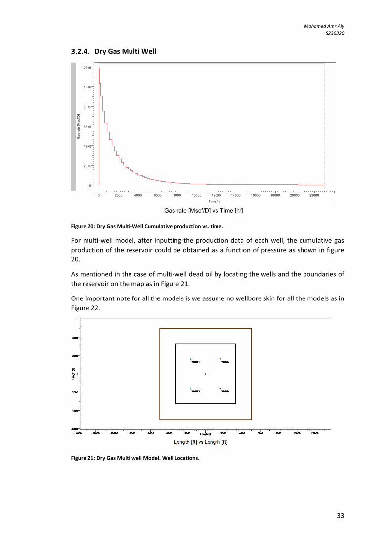
Mohamed Amr Aly

S236320

33

Dry Gas Multi Well

Figure 20: Dry Gas Multi-Well Cumulative production vs. time.

For multi-well model, after inputting the production data of each well, the cumulative gas

production of the reservoir could be obtained as a function of pressure as shown in figure

20.

As mentioned in the case of multi-well dead oil by locating the wells and the boundaries of

the reservoir on the map as in Figure 21.

One important note for all the models is we assume no wellbore skin for all the models as in

Figure 22.

Figure 21: Dry Gas Multi well Model. Well Locations.

0

2E+5

4E+5

6E+5

8E+5

1E+6

1.2E+6

Gas

rate

[Msc

f/D]

Prod

uctio

n [M

scf/D

]

0 2000 4000 6000 8000 10000 12000 14000 16000 18000 20000 22000

Time [hr]

Gas rate [Mscf/D] vs Time [hr]

Mohamed Amr Aly

S236320

34

The model in multiwell case is set numerically.

Figure 22: Dry Gas Multi-well Numerical model Description

Mohamed Amr Aly

S236320

35

3.3. Flowing Material Balance

Dead Oil

To establish the FMB for dead oil we use the approach introduced by (Mattar & Anderson,

2005). This Approach is valid for constant/variable flow rate conditions in which he replaced

the production time with the material balance time previously introduced by (Palacio &

Blasingame, 1993). The approach aims to estimate the original oil in place using the fluid

flow equation in pseudo steady state conditions and combining it with the depletion

equation for dead oil reservoirs.

Starting from liquid flow equation in Porous medium in Pseudo-Steady State Conditions, See

Appendix A:

𝑝𝑤𝑓 = �̅� − 𝑞o 𝜇𝑜4 𝜋𝑘ℎ

[ln 2.25 𝐴

𝐶𝐴𝑟𝑤2 ] Equation 3-1

Setting Dietz factor for a single well symmetrically located in a rectangular drainage area as

30.9

Using the Material Balance equation for dead oil reservoir above bubble point (Depletion

Equation):

𝑝𝑖 − �̅� =𝑞𝑜𝑡

𝑐𝑜𝐴ℎ𝜙 Equation 3-2

𝑝𝑖 − �̅� =𝑞𝑜𝑡

𝑁𝑐𝑜 Equation 3-3

By combining the two equations we reach


𝑐𝑜𝑁+ 141.2 𝑞𝑜𝐵𝑜𝜇𝑜

𝑘ℎ[ln 2.25

𝐴


This can be written as:


𝑐𝑜𝑁+ 𝑏𝑝𝑠𝑠 𝑞𝑜 Equation 3-5

Where bpss (The Pseudo-Steady State Constant), (the reciprocal of productivity index):

𝑏𝑝𝑠𝑠 = 141.2 𝐵𝑜𝜇𝑜

𝑘ℎ[ln 2.25

𝐴


This is constant and was first presented by Blasingame. It can be obtained by rearranging the

equation into:


𝑞𝑜=

𝑞𝑜𝑡

𝑐𝑜𝑁𝑞𝑜+ 𝑏𝑝𝑠𝑠 =

𝑁𝑝𝑐𝑜𝑁𝑞𝑜


This equation is only valid for constant flow rate, however by replacing the production time

with Material Balance time Equation 2-5


𝑞𝑜=

𝑞𝑜𝑡𝑐𝑐𝑜𝑁𝑞𝑜

+ 𝑏𝑝𝑠𝑠 = 𝑡𝑐𝑐𝑜𝑁


Mohamed Amr Aly

S236320

36

A Cartesian plot of (𝑃𝑖−𝑃𝑤𝑓)

𝑞𝑜 vs. 𝑡𝑐 will yield a straight line with an intercept of bpss. Then

Average Pressure could be obtained by:

�̅� = 𝑃𝑤𝑓 + 𝑏𝑝𝑠𝑠 ∗ 𝑞𝑜 Equation 3-9

A Cartesian plot of (𝑝𝑖 − �̅�) vs. 𝑁𝑝

𝐶𝑜 will yield a straight line with a slope equal to

1

𝑁.

Anderson 2005 used the compressibility of the oil 𝑐𝑜. However, further developments of the

flowing material balance showed the same approach but using the total compressibility 𝑐𝑡

instead of the oil compressibility. In this study we developed the oil in place using the two

approaches to study the effect of the compressibility on the total oil in place.

Note that in the Flowing Material Balance for oil, the fluid properties over the production life

(Production period) are assumed to be constant.

For single well, the production data is analyzed and fully representing the whole reservoir.

Therefore, N represents the Initial Oil in place of whole reservoir.

For Multi well, the production data is obtained from four different wells. Therefore, the N

from the analysis of one set of production data represents the approximate drainage area of

this well. In the development of multi-well approach, we assumed that the production of the

4 wells started at the same, wells are symmetrically distributed in the reservoir boundary

and boundary is constant, hence pressure disturbance is uniform.

Dry Gas

In reality, the production data is obtained from the daily flow rate at the surface and

Permanent Down Hole Gauges (PDG) in front of the perforation just to have a valid correct

representing bottom-hole pressure for the representing production flow rate. The use of

Downhole Gauges helped reservoir engineers to establish the way for Rate Transient

Analysis and deep analysis of production data. However, the use of permanent downhole

Gauges are not widely used because of its cost. Other ways of obtaining the bottom-hole

pressure from the well head pressure have showed their applicability as well using

correlations and pressure loss equations to estimate Pwf.

The development of the Flowing material balance for gas reservoir does not only require the

production flowing data, but also the representing PVT data for each production data to

account for the change of the gas properties change with the continuous production. That is

why (Mattar & Anderson, 2005) introduced another function called the material balance

pseudo time to account for gas properties change with time. Equation 2-8

𝑡𝑐𝑎 = (𝜇𝑔𝑐𝑡)𝑖𝑞𝑔

∫𝑞𝑔

𝜇𝑔𝑐𝑡̅̅ ̅̅ ̅̅

𝑡

0


To overcome this point, we have used the PVT data imported from Ecrin database related to

the reservoir and gas properties (Pi, T, Gas Gravity and Gas composition) to build polynomial

equations representing each property as a function of pressure, therefore we could have a

representing set of PVT for the production data at each time step.

The another difference between FMB gas and FMB oil is the use of the pseudo pressure

function instead of the pressure when it comes to gas, hence, the building of polynomial

Mohamed Amr Aly

S236320

37

y = -4.1080E-03x3 + 5.8980E+01x2 + 9.0673E+04x - 1.0519E+08

0

200000000

400000000

600000000

800000000

1E+09

1.2E+09

1.4E+09

0 1000 2000 3000 4000 5000 6000

m(p

), (

Psi

2/c

p)

Pressure (psia)

Pseudo Pressure Function

Figure 23: Pseudo Pressure Function polynomial equation as a funcation of pressure

equations between pressure and pseudo pressure function to be easily able to have values

of m(p) at different P values and vice versa.

The estimation of the fluid properties at the representing time step or the production points

needs to have the average pressure value. However, the method introduced aims to

overcome the main obstacle of conventional material balance which is obtaining the average

reservoir pressure by shutting the well in. Therefore we build an iterative method based on

initial assumption of the G value from which we can further obtain the average reservoir

pressure at the different cumulative production using the conventional gas material balance

equation and then we calculate the gas properties to be able to estimate the gas pseudo

material balance function to implement the FMB for gas and obtain the initial Gas in place.

We iterate until we reach a final value of G that represents the Gas initial in place for the

reservoir.

Generating PVT data represents the production data at each time step

To convert the Pressure values into pseudo pressure function m (p), from the Ecrin PVT

Import option we have a P & m (p) values representing our reservoir. Therefore, we build a

polynomial equation to be able to get m (p) at any value of P.

We chose only the range of pressure we are interested in to have the best fit and we

developed a polynomial equation from the third order for better approximation.

After obtaining 𝑚(�̅�) from the FMB plot, we need to convert it to average pressure to build

the conventional Material Balance equation for Gas. We us the polynomial equation

developed in Figure 24.

Mohamed Amr Aly

S236320

38

y = 3.142E-25x3 - 1.098E-15x2 + 3.964E-06x + 9.880E+02

0

1000

2000

3000

4000

5000

6000

0 500000000 1E+09 1.5E+09

Pre

ssu

re (

psi

a)

m(p), (psia2/cp)

Pseudo Pressure Function

Figure 24: Average Reservoir Pressure polynomial equation as a function of gas pseudo

pressure.

y = 1.177E-04x2 + 2.175E-01x + 9.549E+02

0

500

1000

1500

2000

2500

3000

3500

4000

4500

5000

0 1000 2000 3000 4000 5000

P

P/z

P/Z vs P

Figure 25: Average Reservoir Pressure Polynomial Equation as a Function of P/Z.

From Step (2) in the Gas FMB procedure, we obtain P/Z values at different Gp values.

However, we need to obtain the average pressure to calculate the gas properties at this

value. Therefore, again from the PVT data imported from Ecrin Database representing our

reservoir. We get P/z values and then build a function of P from these P/z values as shown in

Figure 25. We chose on the range of pressure in our interest for better fitting the polynomial

equation (2500: 4600 Pisa).

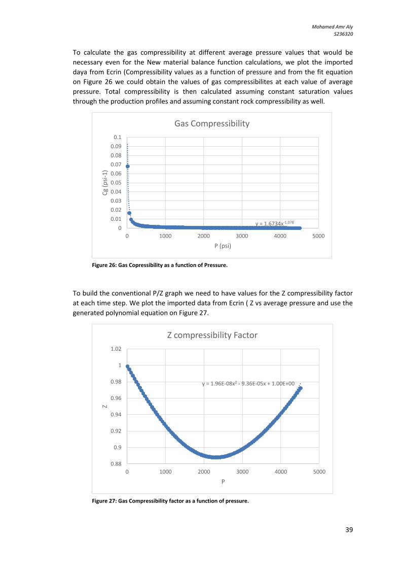
Mohamed Amr Aly

S236320

39

Figure 26: Gas Copressibility as a function of Pressure.

Figure 27: Gas Compressibility factor as a function of pressure.

y = 1.6734x-1.078

0

0.01

0.02

0.03

0.04

0.05

0.06

0.07

0.08

0.09

0.1

0 1000 2000 3000 4000 5000

Cg

(psi

-1)

P (psi)

Gas Compressibility

y = 1.96E-08x2 - 9.36E-05x + 1.00E+00

0.88

0.9

0.92

0.94

0.96

0.98

1

1.02

0 1000 2000 3000 4000 5000

Z

P

Z compressibility Factor

To calculate the gas compressibility at different average pressure values that would be

necessary even for the New material balance function calculations, we plot the imported

daya from Ecrin (Compressibility values as a function of pressure and from the fit equation

on Figure 26 we could obtain the values of gas compressibilites at each value of average

pressure. Total compressibility is then calculated assuming constant saturation values

through the production profiles and assuming constant rock compressibility as well.

To build the conventional P/Z graph we need to have values for the Z compressibility factor

at each time step. We plot the imported data from Ecrin ( Z vs average pressure and use the

generated polynomial equation on Figure 27.

Mohamed Amr Aly

S236320

41

y = -5E-14x3 + 6E-10x2 + 1E-06x + 0.0129

0

0.005

0.01

0.015

0.02

0.025

0.03

0 1000 2000 3000 4000 5000

Vis

cosi

ty M

ug

(cp

)

Pressure (Psi)

Gas Viscosity

For the gas viscosity, the same technique is also developed and the polynomial equation

representing the range we are interested in on Figure 28 is used for generating the gas

viscosity values at different average pressure values.

3.3.2.1. Gas Flowing Material Balance

The method used is based on driving the FMB equation from the fluid flow equation and

combining it with the conventional material balance equation as proposed by (Mattar &

Anderson, 2005).

The first approach introduced by (McNeil, 1995) needs to have valid PVT data representing

the production points because it is mainly Pwf/Z plotting vs Gp. Therefore, the approach we

used to assume an initial G and with the help of the correlation built using PVT database on

Ecrin will not be an appropriate method and might gibe high error.

Starting from the gas flow equation in a porous medium in pseudo steady conditions in

Appendix A

𝑚(𝑝𝑤𝑓 ) = 𝑚(�̅�) −𝑞𝑔 𝑇

2𝜋 𝑘 ℎ (𝑃𝑠𝑐𝑇𝑠𝑐) [ln 2.25

𝐴


Setting Dietz factor for a single well symmetrically located in a rectangular drainage area as

30.9 Using the material balance equation for gas introduced (Mattar & Anderson, 2005)*

𝑚(𝑝𝑖) − 𝑚(�̅�) =2𝑝𝑖𝑞𝑔 𝑡𝑐𝑎

𝐺𝑍𝑖𝐶𝑡𝑖𝜇𝑔𝑖 Equation 3-11

Equation 3-11 mentioned in literature without the term (C𝜇𝑖) in the dominator. However,

the same equation was found in other literatures (Morad & Clarkson, 2006) indicating to the

missing term.

Figure 28: Gas viscosity as a function of pressure.

Mohamed Amr Aly

S236320

41

Combining the two equations we reach:

𝑚(𝑝𝑖) − 𝑚(𝑝𝑤𝑓) = 2𝑝𝑖𝑞𝑔 𝑡𝑐𝑎

𝐺𝑍𝑖𝐶𝑡𝑖𝜇𝑔𝑖+

𝑞𝑔 𝑇


𝐴


𝑚(𝑝𝑖) −𝑚(𝑝𝑤𝑓)

𝑞𝑔=

2𝑝𝑖 𝑡𝑐𝑎𝐺𝑍𝑖𝐶𝑡𝑖𝜇𝑖

+ 𝑏𝑎,𝑝𝑠𝑠 Equation 3-13

𝑚(�̅�) = 𝑚(𝑝𝑤𝑓) + 𝑞𝑔 𝑏𝑎,𝑝𝑠𝑠 Equation 3-14

Where, 𝑏𝑎,𝑝𝑠𝑠 = 𝑇


𝐴


From 𝑏𝑝𝑠𝑠, we can have an estimation of the gas effective permeability k if we know h.

By plotting 𝑚(𝑝𝑖)−𝑚(𝑝𝑤𝑓)

𝑞𝑔 vs 𝑡𝑐𝑎 we get 𝑏𝑎,𝑝𝑠𝑠 as intercept. Then we get 𝑚(�̅�). Which is

converted to Pavg to build the conventional P/z plot.

𝑡𝑐𝑎 , here is developed from the explicit Pseudo material balance function. Equation 2-8

Comparison between the two methods is developed to see the effect on calculating the

permeability and the gas in place.

Gas FMB Steps in the thesis work:

1) Assume an initial value of G. This depends on the production profile. Assume that

total Gp=30% of G.

2) Use Conventional Material Balance (P/Z) Equation for Gas to obtain the average

reservoir pressure at each time step.

3) Calculate the gas properties at this Pavg (Viscosity & Gas compressibility)

4) Calculate the material balance time function tca.

5) Convert all pressures in pseudo pressure function (Pwf & Pavg).

6) Plot 𝑚(𝑝𝑖)−𝑚(𝑝𝑤𝑓)

𝑞𝑔 𝑣𝑠 𝑡𝑐𝑎 to obtain ba,pss as an intercept

7) Get 𝑚(�̅�) = 𝑚(𝑝𝑤𝑓) + 𝑞𝑔𝑏𝑎,𝑝𝑠𝑠

8) Convert 𝑚(�̅�) into P avg and build the Pavg/Z graph o obtain Gi.

9) Repeat until we reach the real value of G.

3.3.2.2. Agarwal Gardner Method

By Plotting the normalize flow rate vs the normalized cumulative to have the initial gas in

place as the intercept of x-axis. Equation 2-23 & Equation 2-24.

3.3.2.3. New Pseudo Material Balance time function

This approach needs to convert the pseudo pressure function into normalized pseudo

pressure function.

Mohamed Amr Aly

S236320

42

𝑑𝑚(�̅�)𝑛 =(𝜇𝑔𝑍)𝑖𝑃𝑖

�̅�

�̅��̅�𝑑�̅� Equation 3-16

Then plotting 𝑞𝑔

𝑚(𝑃𝑖)𝑛− 𝑚(𝑃𝑤𝑓)𝑛 vs

𝑞𝑔

𝐺𝑝𝑛 we obtain 𝐺 as intercept. See Flowing Material Balance

using a new Pseudotime function

𝑇𝑎 = 1

𝑞𝑔∫

(𝜇𝑔𝑐𝑡)𝑖𝜇𝑔̅̅ ̅𝑐�̅�

𝐺𝑝

0

𝑑𝐺𝑝 Equation 3-17

𝐺𝑝𝑛 = ∫(𝜇𝑔𝑖𝐶𝑡𝑖)


𝐺𝑝

0

Equation 3-18

𝑇𝑎 =𝐺𝑝𝑛

𝑞𝑔 Equation 3-19

𝑇𝑎, is defined as the new pseudo material balance function. The calculating of 𝐺𝑝𝑛is done by

fitting the polynomial equation of the (𝜇𝑔𝑖𝐶𝑡𝑖)

𝜇𝑔̅̅ ̅̅ 𝐶𝑡̅̅ ̅ term at different pressures as a function of the

cumulative production as shown in Figure 29.

Figure 29: Viscosity compressibility ratio as a function of cumulative production.

The steps were followed as explained in the Flowing Material Balance using a new

Pseudotime function section (P. 20 & 21).

The comparison between the three methods of FMB introduced here is performed with a

close comparison on the effect on the different calculation approaches of pseudo material

balance function and the pseudo normalized cumulative function.

Mohamed Amr Aly

S236320

43

Chapter 4 Results & Discussion The main purpose of the study is to estimate the Initial Hydrocarbon in place for the

different models by validating two approaches; Rate Transient Analysis & Flowing Material

Balance to prove that Production Data could be used to estimate the hydrocarbon in place

without the need to shut the well in and implementing the conventional methods. These

approaches aim to show how close the results obtained from these approaches to the most

valid one (Numerical simulation model).

RTA provides us with information about the boundaries of the reservoir and when

stabilization occurs. This helps us to make sure that we are in pseudo steady state conditions

as the flowing Material balance is valid when the production reaches the pseudo steady

conditions when all boundaries are touched and depletion starts to occur. One important

note is here we are working on single phase production in explicit depletion conditions (No

water drive, no gas in solution or gas cap expansion).

The results we have from this study are:

Numerical simulation model HOIP estimation.

Rate Transient Analysis (RTA):

Ecrin, Topaze Model Match

Fetkovich Type-curves Match

Blasingame Type-curves Match

Flowing Material Balance (FMB):

Dead Oil: using Material balance time

- Using total compressibility

- Using oil compressibility

Dry Gas:

- Using Pseudo Material Balance Function

- Using Normalized Rate – Normalized Cumulative Approach

- Using Normalized Pseudo Cumulative Function

Comparing these results will tell us how far we are from the exact value and what the error

percentage for each case is.

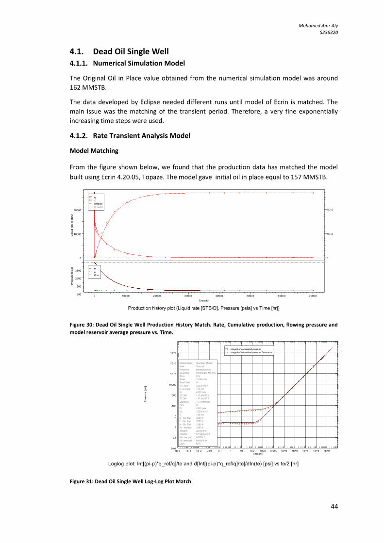
Mohamed Amr Aly

S236320

44

4.1. Dead Oil Single Well

Numerical Simulation Model

The Original Oil in Place value obtained from the numerical simulation model was around

162 MMSTB.

The data developed by Eclipse needed different runs until model of Ecrin is matched. The

main issue was the matching of the transient period. Therefore, a very fine exponentially

increasing time steps were used.

Rate Transient Analysis Model

Model Matching

From the figure shown below, we found that the production data has matched the model

built using Ecrin 4.20.05, Topaze. The model gave initial oil in place equal to 157 MMSTB.

Figure 30: Dead Oil Single Well Production History Match. Rate, Cumulative production, flowing pressure and

model reservoir average pressure vs. Time.

Figure 31: Dead Oil Single Well Log-Log Plot Match

0

40000

80000

Liqu

id ra

te [S

TB/D

]

0

4E+6

8E+6

Liqu

id v

olum

e [S

TB]

q

Q

q model

Q model

0 10000 20000 30000 40000 50000 60000 70000

Time [hr]

500

1500

2500

3500

Pres

sure

[psi

a] Pi

p

Pbar

Production history plot (Liquid rate [STB/D], Pressure [psia] vs Time [hr])

1E-5 1E-4 1E-3 0.01 0.1 1 10 100 1000 10000 1E+5 1E+6 1E+7 1E+8 1E+9Time [hr]

0.01

0.1

1

10

100

1000

10000

1E+5

1E+6

1E+7

Pres

sure

[psi

]

Integral of normalized pressure

Integral of normalized pressure Derivative

Model Option Standard Model

Well Vertical

Reservoir Homogeneous

Boundary Rectangle, No flow

Tmin 0 hr

Tmax 70149.4 hr

Total Skin 0

k.h, total 32200 md.ft

k, average 196 md

Pi 4500 psia

STOIIP 157 MMSTB

STOIP 147 MMSTB

Qo(tmax) 10.7 MMSTB

Skin 0

Pi 4500 psia

k.h 32200 md.ft

k 196 md

S - No flow 3280 ft

E - No flow 3280 ft

N - No flow 3280 ft

W - No flow 3280 ft

TMatch 22700 [hr]-1

PMatch 0.194 [psia]-1

Ab. rate (qa) 0 STB/ D

Ab. time (ta) 69069.8 hr

Q(ta) N/ A

Loglog plot: Int[(pi-p)*q_ref/q]/te and d[Int[(pi-p)*q_ref/q]/te]/dln(te) [psi] vs te/2 [hr]

Mohamed Amr Aly

S236320

45

This graph shows that the late part of the data is already in the pseudo steady state

conditions that we are in interest of. The log-log plot of the integral of the normalized

pressure and its derivative also confirms the same results obtained from the model.

Figure 32: Dead Oil Single Well Model Blasingame Plot Match.

Figure 33: Dead Oil Single Well Model Fetkovich Plot Match.

From the Fetkovich Plot of the model we can confirm that Pseudo Steady State conditions

already reached after around 2000 hr of the production.

The model shows around 3.00% of error between the numerical simulation model and the

RTA model.

1E-4 1E-3 0.01 0.1 1 10 100 1000 10000 1E+5 1E+6 1E+7 1E+8 1E+9 1E+10Time [hr]

1E-9

1E-8

1E-7

1E-6

1E-5

1E-4

1E-3

0.01

0.1

Pres

sure

-1 [[

psi]-

1]

PI

PI Int.

PI Int. Derivative


Well Vertical



Tmin 0 hr

Tmax 70149.4 hr

Total Skin 0


k, average 196 md

Pi 4500 psia

STOIIP 157 MMSTB

STOIP 147 MMSTB

Qo(tmax) 10.7 MMSTB

Skin 0

Pi 4500 psia

k.h 32200 md.ft

k 196 md

S - No flow 3280 ft

E - No flow 3280 ft

N - No flow 3280 ft

W - No flow 3280 ft

TMatch 22700 [hr]-1




Q(ta) N/ A

Blasingame plot: q/q_ref/(pi-p), Int[q/q_ref/(pi-p)]/te and d[Int[q/q_ref/(pi-p)]/te]/dlnte [[psi]-1] vs te [hr]

1E-4 1E-3 0.01 0.1 1 10 100 1000 10000 1E+5 1E+6Time [hr]

0.01

0.1

1

10

100

1000

10000

1E+5

Liqu

id ra

te [S

TB/D

]

1

10

100

1000

10000

1E+5

1E+6

1E+7

Liqu

id v

olum

e [S

TB]


Well Vertical



Tmin 0 hr

Tmax 70149.4 hr

Total Skin 0


k, average 196 md

Pi 4500 psia

STOIIP 157 MMSTB

STOIP 147 MMSTB

Qo(tmax) 10.7 MMSTB

Skin 0

Pi 4500 psia

k.h 32200 md.ft

k 196 md

S - No flow 3280 ft

E - No flow 3280 ft

N - No flow 3280 ft

W - No flow 3280 ft

TMatch 22700 [hr]-1




Q(ta) N/ A

Fetkovich plot: q [STB/D], Q [STB] vs dt [hr]

Mohamed Amr Aly

S236320

46


Figure 34: Dead Oil Single Well Fetkovich Type-curves Match

From the match of the production data with Fetkovich Type-curves, we obtain OOIP as

around 160 MMSTB with permeability 198 mD. Comparing these results with the numerical

simulation model;

Table 13: Comparison between results obtained by Fetkovich Type-curves match and Numerical Simulation

Model.

Models OOIP (MMSTB) Permeability (md)

Numerical Simulation 162 200

Fetkovich Type-curves 160 198

Comparing the results with the numerical simulation values, we obtain an error ~ 1.25 %.

Blasingame Type-curves Match

Figure 35: Dead Oil Single Well Blasingame Type-curves Match.

1E-4 1E-3 0.01 0.1 1 10Not a unit

1E-3

0.01

0.1

1

Not

a u

nit

Re/ rwa=10

Re/ rwa=20

Re/ rwa=50

Re/ rwa=100

Re/ rwa=200

Re/ rwa=1000

Re/ rwa=10000

Re/ rwa=100000

exp(-tDd)

b=0

b=0.1

b=0.2

b=0.3

b=0.4

b=0.5

b=0.6

b=0.7

b=0.8

b=0.9

b=1

b 0

Di 0.00461 [Day]-1

qi 50200 STB/ D

UR 10.9 MMSTB

pwf 900 psia

k.h 32500 md.ft

k 198 md

Re 3730 ft

rwa 1.07 ft

Skin -0.474

PV 255 MMB

STOIIP 160 MMSTB

STOIP 149 MMSTB

Fetkovich type curve plot: qDd and QDd vs tDd

1E-4 1E-3 0.01 0.1 1 10 100Not a unit

0.01

0.1

1

10

Not

a u

nit

Re/ rwa=4

Re/ rwa=12

Re/ rwa=28

Re/ rwa=80

Re/ rwa=160

Re/ rwa=800

Re/ rwa=5598.42

Re/ rwa=10000

qDd

qDdi

qDdid

STOIIP 163 MMSTB

STOIP 152 MMSTB

Re 3770 ft

rwa 0.673 ft

k.h 35900 md.ft

k 219 md

Skin -0.00929

Blasingame type curve plot: qDd, qDdi and qDdid vs tDd

Mohamed Amr Aly

S236320

47

Figure 36: Dead Oil Single Well FMB, bpss is obtained as the Y-intercept of the straight line

y = 4.362E-04x + 5.191E-02

0

2000

4000

6000

8000

10000

12000

0 5000000 10000000 15000000 20000000 25000000

Pi-

Pw

f/q

Material Balance Time tc

Estimation of bpss

The match of the production data with Blasingame’s Type-curves showed OOIP as ~163

MMSTB with an over estimation of permeability as 219 mD (Which still in the same order of

magnitude).

Flowing Material Balance

For Dead Oil, the most critical issue is to have a valid PVT data representing the production

data of your reservoir. As we have mentioned that for Dead Oil FMB the PVT data is

considered constant over the production profile. Therefore, the oil compressibility, oil

viscosity and oil formation volume factor are considered constants.

Table 14: Dead Oil Single Well PVT Data used in RTA & FMB

Pi (psia) 4500

viscosity (cp) 1.8

co psia-1 1.26E-05

ct psia-1 1.42E-05

Bo 1.2

Our area is represented by a rectangle (2000m*2000m) with a net pay thickness of 50 m.

Therefore with setting a well in the center we get a Dietz Shape factor as 30.9. This is

important in calculating the reservoir permeability from the Pseudo Steady State Constant

(bpss).

From the graph we get:

Table 15: Dead Oil Single Well, reservoir permeability using FMB approach.

bpss 5.19E-02 psia/STB/D

Kh 3.94E+04 mD.ft

k 240 mD

Mohamed Amr Aly

S236320

48

Figure 37: Dead Oil Single Well Flowing Material Balance using Oil Compressibility

y = 5.602E-09x

0

500

1000

1500

2000

2500

3000

3500

4000

0.00E+00 2.00E+11 4.00E+11 6.00E+11 8.00E+11

Pi-

Pav

g (p

si)

Np/Co

Flowing Material Balance Oil [Oil Compressibility]

y = 6.314E-09x

0

500

1000

1500

2000

2500

3000

3500

4000

0.00E+00 2.00E+11 4.00E+11 6.00E+11 8.00E+11

Pi-

Pav

g (p

si)

Np/ct

Flowing Material Balance [Total Compressibility]

We notice that the value of the permeability from the Flowing material balance approach is

over estimated by around 20%

From bPss we get Pavg to plot 𝑃𝑖−�̅�

𝑞 vs

𝑁𝑝

𝑐 to get the Original Oil in place as

1

𝑠𝑙𝑜𝑝𝑒 . The first

values representing the transient period where they do not follow the straight line.

From Figure 37, we get the slope as 1/N which gives N equal to 178.5 MMSTB

Figure 38 shows theat the slope increased when using the total compressibility which in

return gives N as 158.5 MMSTB. This value is more reliable comparing with the numerical

simulation model.

Figure 38: Dead Oil Single Well Flowing Material Balance using total Compressibility.

Mohamed Amr Aly

S236320

49

Table 16: Dead Oil Single Well OOIP comparison between the different approaches.

Therefore, we see that the approach introduced by (Mattar & Anderson, 2005) that using

total compressibility instead of the oil compressibility gives better estimation of the oil in

place.

4.2. Dead Oil Multi Well Numerical Simulation Model

The same model with the same parameters have been used for the multi-well case.

Therefore, the same value of OOIP from the numerical simulation model was obtained as ~

162 MMSTB.

The same time steps used for the single model was also implemented in this case to match

the cumulative production cure in Topaze in the transient period.

Rate Transient Analysis

Model Matching

The model built using Topaze for the 4 wells matched the production data and gave the

same result provided by the single well as ~ 157 MMSTB.

Figure 39: Dead Oil Multi Well Cumulative Production vs. time.

0

50000

1E+5

1.5E+5

2E+5

2.5E+5

Liqu

id ra

te [S

TB/D

]

Prod

uctio

n [S

TB/D

]

0 400 800 1200 1600 2000 2400 2800 3200 3600

Time [hr]

Liquid rate [STB/D] vs Time [hr]


RTA Model Blasingame type-curve plot

Fetkovich type-curve plot

FMB Total C

OOIP 162 MMSTB 157 MMSTB 163 MMSTB 160 MMSTB 158.5

K 200 mD 198 mD 219 mD 196 mD 240

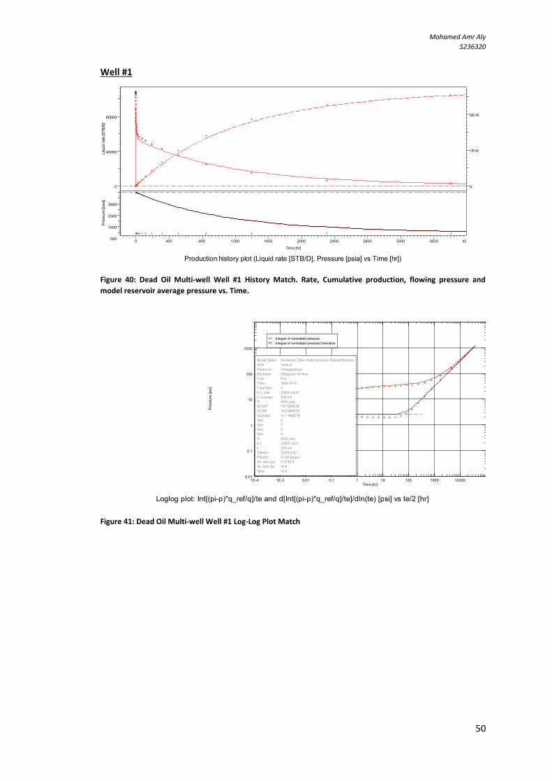
Mohamed Amr Aly

S236320

51

Well #1

Figure 40: Dead Oil Multi-well Well #1 History Match. Rate, Cumulative production, flowing pressure and


Figure 41: Dead Oil Multi-well Well #1 Log-Log Plot Match

0

40000

80000

Liqu

id ra

te [S

TB/D

]

0

1E+6

2E+6

Liqu

id v

olum

e [S

TB]

0 400 800 1200 1600 2000 2400 2800 3200 3600 4000

Time [hr]

500

1500

2500

3500

Pres

sure

[psi

a]


1E-4 1E-3 0.01 0.1 1 10 100 1000 10000Time [hr]

0.01

0.1

1

10

100

1000

Pres

sure

[psi

]



Model Option Numerical, Other Wells Included, Material Balance

Well Vertical


Boundary Polygonal, No flow

Tmin 0 hr

Tmax 3804.97 hr

Total Skin 0


k, average 200 md

Pi 4500 psia

STOIIP 157 MMSTB

STOIP 147 MMSTB

Qo(tmax) 10.1 MMSTB

Skin 0

Skin 0

Skin 0

Skin 0

Pi 4500 psia

k.h 32800 md.ft

k 200 md

TMatch 23200 [hr]-1



Ab. time (ta) N/ A

Q(ta) N/ A


Mohamed Amr Aly

S236320

51

Figure 42: Dead Oil Multi-well Well #1 Model Blasingame Plot Match.

Figure 43: Dead Oil Multi-well Well #1 Model Fetkovich Plot Match.

From both the Log-Log Plot and Fetkovich plot match of the model we confirm that the late

period of production for the well is already in the pseudo steady state conditions.

In our study we focus only on how the production data could be analyzed to provide

estimation on the hydrocarbon in place, therefore skin is set equal to zero.

The Match of the model plots (Log-Log, Blasingame, Fetkovich) with the production data

confirms the validation of the model built with the production data of each well and also the

estimation of the OOIP.

1E-4 1E-3 0.01 0.1 1 10 100 1000 10000Time [hr]

1E-5

1E-4

1E-3

0.01

0.1

Pres

sure

-1 [[

psi]-

1]

PI

PI Int.

PI Int. Derivative


Well Vertical



Tmin 0 hr

Tmax 3804.97 hr

Total Skin 0


k, average 200 md

Pi 4500 psia

STOIIP 157 MMSTB

STOIP 147 MMSTB

Qo(tmax) 10.1 MMSTB

Skin 0

Skin 0

Skin 0

Skin 0

Pi 4500 psia

k.h 32800 md.ft

k 200 md

TMatch 23200 [hr]-1



Ab. time (ta) N/ A

Q(ta) N/ A


1E-7 1E-6 1E-5 1E-4 1E-3 0.01 0.1 1 10 100 1000 10000 1E+5Time [hr]

10

100

1000

10000

1E+5

1E+6

1E+7

Liqu

id ra

te [S

TB/D

]

1

10

100

1000

10000

1E+5

1E+6

Liqu

id v

olum

e [S

TB]


Well Vertical



Tmin 0 hr

Tmax 3804.97 hr

Total Skin 0


k, average 200 md

Pi 4500 psia

STOIIP 157 MMSTB

STOIP 147 MMSTB

Qo(tmax) 10.1 MMSTB

Skin 0

Skin 0

Skin 0

Skin 0

Pi 4500 psia

k.h 32800 md.ft

k 200 md

TMatch 23200 [hr]-1



Ab. time (ta) N/ A

Q(ta) N/ A


Mohamed Amr Aly

S236320

52


Figure 44: Dead Oil Multi-well Well #1 Fetkovich Type-curves Match.

From Fetkovich Type-curves match we obtain the OOIP in the drainage area of each well. For

well #1 we obtain ~ 38.7 MMSTB

Blasingame Type-curves

Figure 45: Dead Oil Multi-well Well #1 Blasingame Type-curves Match.

The match of the Blasingame type-curve gives an estimation of the OOIP stored in the

drainage area covered by each well. For Well #1, it gives ~ 39.7 MMSTB

1E-4 1E-3 0.01 0.1 1 10Not a unit

1E-3

0.01

0.1

1

Not

a u

nit

Re/ rwa=10

Re/ rwa=20

Re/ rwa=50

Re/ rwa=100

Re/ rwa=200

Re/ rwa=1000

Re/ rwa=10000

Re/ rwa=100000

exp(-tDd)

b=0

b=0.1

b=0.2

b=0.3

b=0.4

b=0.5

b=0.6

b=0.7

b=0.8

b=0.9

b=1 b 0

Di 0.0208 [Day]-1

qi 54700 STB/ D

UR 2.64 MMSTB

pwf 900 psia

k.h 35700 md.ft

k 218 md

Re 1840 ft

rwa 0.501 ft

Skin 0.286

PV 61.9 MMB

STOIIP 38.7 MMSTB

STOIP 28.6 MMSTB


1E-4 1E-3 0.01 0.1 1 10 100Not a unit

0.01

0.1

1

10

Not

a u

nit

Re/ rwa=4

Re/ rwa=12

Re/ rwa=28

Re/ rwa=80

Re/ rwa=160

Re/ rwa=800

Re/ rwa=3177.13

Re/ rwa=10000

qDd

qDdi

qDdid

STOIIP 39.7 MMSTB

STOIP 29.6 MMSTB

Re 1860 ft

rwa 0.586 ft

k.h 37100 md.ft

k 226 md

Skin 0.129


Mohamed Amr Aly

S236320

53


The same approach used for single well is implemented for the production data of each well separately to give an estimation of the OOIP covered by the drainage area of each well.

The PVT data for the single well with the same assumption of constant PVT over the production period are considered.

Table 17: Dead Oil Multi-well Well #1 Well PVT Data used in RTA & FMB

The only difference in this analytical approach is the Dietz Shape factor regarding the

multiwall case as in the single well it was only a symmetrically centered well in a rectangular

area. However, here we have 4 wells; considering the new Dietz Shape factor 17.7 for each

well.

Pi (psia) 4500

viscosity (cp) 1.8

co psia-1 1.26E-05

ct psia-1 1.42E-05

Bo 1.2

Figure 46: Dead Oil Multi-well Well #1 FMB, bpss is obtained as the Y-intercept of the straight

line

Mohamed Amr Aly

S236320

54

Figure 47: Dead Oil Multi-well Well #1 Flowing Material Balance using Oil Compressibility

Figure 48: Dead Oil Multi-well Well #1 Flowing Material Balance using Total Compressibility.

Table 18: Dead Oil Multi-well Well #1, reservoir permeability using FMB approach.

bpss 0.0483 psia/STB/D

Kh 44123.43 mD.ft

k 269.0 mD

The permeability estimated by the flowing material balance is over estimated and this might

be because of the neglecting of the skin effect.


𝑞 vs

𝑁𝑝


1



N1= 44.8 MMSTB

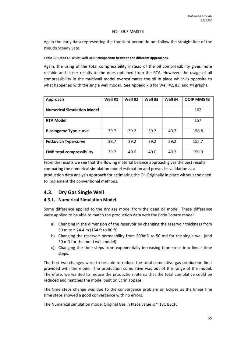
Mohamed Amr Aly

S236320

55

N1= 39.7 MMSTB

Again the early data representing the transient period do not follow the straight line of the

Pseudo Steady Sate.

Table 19: Dead Oil Multi-well OOIP comparison between the different approaches.

Again, the using of the total compressibility instead of the oil compressibility gives more

reliable and closer results to the ones obtained from the RTA. However, the usage of oil

compressibility in the multiwall model overestimates the oil in place which is opposite to

what happened with the single well model. See Appendix B for Well #2, #3, and #4 graphs.

From the results we see that the flowing material balance approach gives the best results

comparing the numerical simulation model estimation and proves its validation as a

production data analysis approach for estimating the Oil Originally in place without the need

to implement the conventional methods.

4.3. Dry Gas Single Well


Some difference applied to the dry gas model from the dead oil model. These difference

were applied to be able to match the production data with the Ecrin Topaze model.

a) Changing in the dimension of the reservoir by changing the reservoir thickness from

50 m to ~ 24.4 m (164 ft to 80 ft)

b) Changing the reservoir permeability from 200mD to 50 md for the single well (and

30 mD for the multi well model).

c) Changing the time steps from exponentially increasing time steps into linear time

steps.

The first two changes were to be able to reduce the total cumulative gas production limit

provided with the model. The production cumulative was out of the range of the model.

Therefore, we wanted to reduce the production rate so that the total cumulative could be

reduced and matches the model built on Ecrin Topaze.

The time steps change was due to the convergence problem on Eclipse as the linear fine

time steps showed a good convergence with no errors.

The Numerical simulation model Original Gas in Place value is ~ 131 BSCF.

Approach Well #1 Well #2 Well #3 Well #4 OOIP MMSTB

Numerical Simulation Model 162

RTA Model 157

Blasingame Type-curve 39.7 39.2 39.2 40.7 158.8

Fetkovich Type-curve 38.7 39.2 39.2 39.2 155.7

FMB total compressibility 39.7 40.0 40.0 40.2 159.9

Mohamed Amr Aly

S236320

56


Model Matching

The match of the analytical model on Ecrin, Topaze showed that the reservoir has ~135

BSCF. For single well model, the analytical or the numerical model Ecri. Topaze will give the

same values. However, for multiwall model it is better to use the numerical model.

Figure 49: Dry Gas Single Well Well #4 History Match. Rate, Cumulative production, flowing pressure and


Again from the log-log plot we confirm that the reservoir has reached the pseudo steady

state conditions when the integral and the integral derivative merge in a straight line with a

unit slope. This is also easily confirmed from the Fetkovich plot. And that is what we need to

confirm to be able to continue our further analysis using the flowing material balance as

well.

Figure 50: Dry Gas Single Well Log-Log Plot Match.

0

1E+5

2E+5

3E+5

Gas

rate

[Msc

f/D]

0

1E+10

2E+10

3E+10

Gas

vol

ume

[scf

]

q

Q

q model

Q model

0 5000 10000 15000 20000 25000 30000 35000 40000 45000 50000

Time [hr]

3200

3700

4200

Pres

sure

[psi

a] Pi

p

Pbar

Production history plot (Gas rate [Mscf/D], Pressure [psia] vs Time [hr])

0.01 0.1 1 10 100 1000 10000 1E+5 1E+6 1E+7 1E+8Time [hr]

100

1000

10000

1E+5

1E+6

1E+7

1E+8

Gas

pot

entia

l [ps

i2/c

p]



Model Option Standard Model, Material Balance

Well Vertical



Tmin 0 hr

Tmax 48000 hr

Total Skin -0.0512


k, average 47.9 md

Pi 4500 psia

STGIIP 149 bscf

STGIP 110 bscf

Qg(tmax) 38.8 bscf

Skin -0.0512

Pi 4500 psia

k.h 3840 md.ft

k 47.9 md

S - No flow 3490 ft

E - No flow 3490 ft

N - No flow 3490 ft

W - No flow 3490 ft

TMatch 41000 [hr]-1

PMatch 0.00132 [psi2/ cp]-1

Ab. rate (qa) 0 Mscf/ D


Q(ta) N/ A

Loglog plot: Int[(m(pi)-m(p))*q_ref/q]/te and d[Int[(m(pi)-m(p))*q_ref/q]/te]/dln(te) [psi2/cp] vs te/2 [hr]

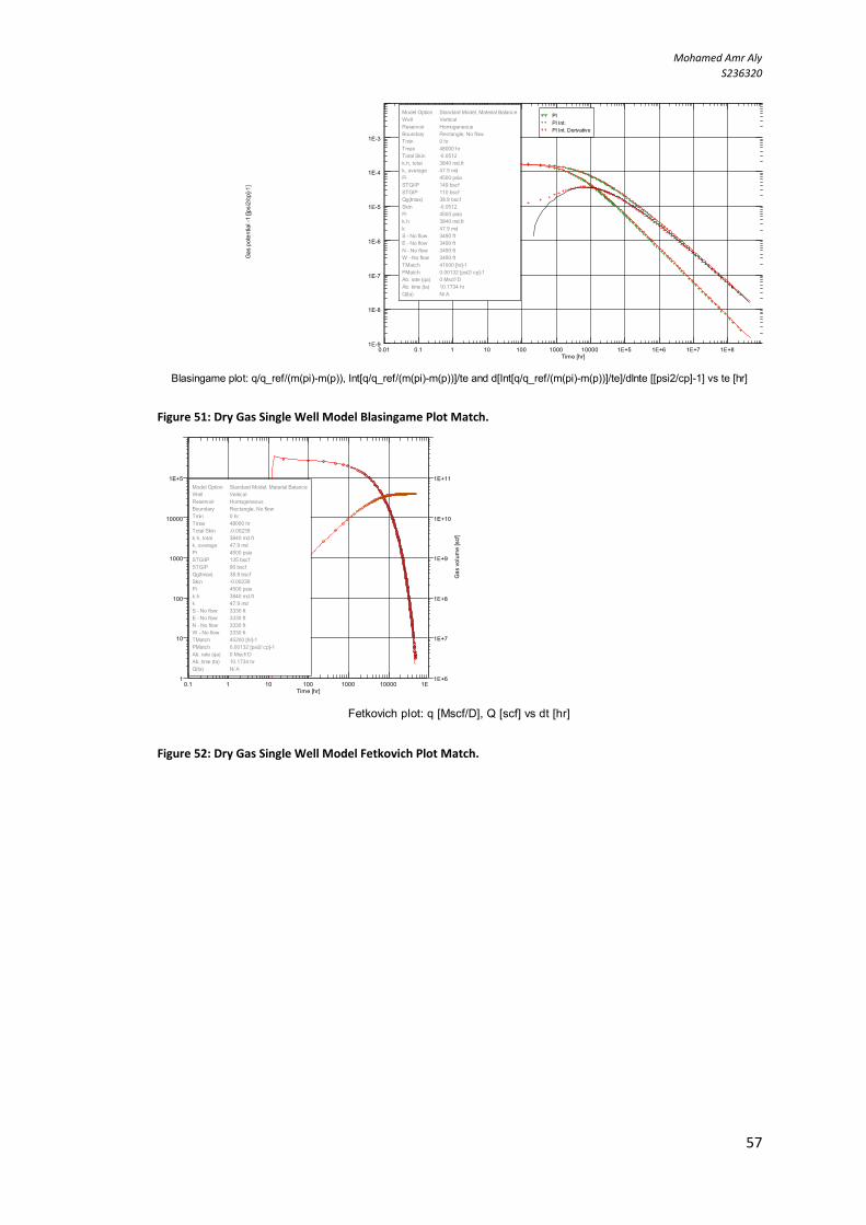
Mohamed Amr Aly

S236320

57

Figure 51: Dry Gas Single Well Model Blasingame Plot Match.

Figure 52: Dry Gas Single Well Model Fetkovich Plot Match.

0.01 0.1 1 10 100 1000 10000 1E+5 1E+6 1E+7 1E+8Time [hr]

1E-9

1E-8

1E-7

1E-6

1E-5

1E-4

1E-3

Gas

pot

entia

l -1

[[psi

2/cp

]-1]

PI

PI Int.

PI Int. Derivative


Well Vertical



Tmin 0 hr

Tmax 48000 hr

Total Skin -0.0512


k, average 47.9 md

Pi 4500 psia

STGIIP 149 bscf

STGIP 110 bscf

Qg(tmax) 38.8 bscf

Skin -0.0512

Pi 4500 psia

k.h 3840 md.ft

k 47.9 md

S - No flow 3490 ft

E - No flow 3490 ft

N - No flow 3490 ft

W - No flow 3490 ft

TMatch 41000 [hr]-1




Q(ta) N/ A

Blasingame plot: q/q_ref/(m(pi)-m(p)), Int[q/q_ref/(m(pi)-m(p))]/te and d[Int[q/q_ref/(m(pi)-m(p))]/te]/dlnte [[psi2/cp]-1] vs te [hr]

0.1 1 10 100 1000 10000 1E+5Time [hr]

1

10

100

1000

10000

1E+5

Gas

rate

[Msc

f/D]

1E+6

1E+7

1E+8

1E+9

1E+10

1E+11

Gas

vol

ume

[scf

]


Well Vertical



Tmin 0 hr

Tmax 48000 hr

Total Skin -0.00239


k, average 47.9 md

Pi 4500 psia

STGIIP 135 bscf

STGIP 96 bscf

Qg(tmax) 38.8 bscf

Skin -0.00239

Pi 4500 psia

k.h 3840 md.ft

k 47.9 md

S - No flow 3330 ft

E - No flow 3330 ft

N - No flow 3330 ft

W - No flow 3330 ft

TMatch 45200 [hr]-1




Q(ta) N/ A

Fetkovich plot: q [Mscf/D], Q [scf] vs dt [hr]

Mohamed Amr Aly

S236320

58


Figure 53: Dry Gas Single Well Fetkovich Type-curves Match.

The match of the production data on Fetkovich Type-curves showed an estimation of OGIP

as ~ 131 BSCF.

Blaingame Type-curves

Figure 54: Dry Gas Single Well Blasingame Type-curves Match.

Also the match of the production data on Blasingame Type-curves gave the same result as ~

131 BSCF which confirms the validation of the RTA as an approach for dry gas reservoir to

give an estimation of the OGIP.

1E-4 1E-3 0.01 0.1 1 10Not a unit

1E-3

0.01

0.1

1

Not

a u

nit

Re/ rwa=10

Re/ rwa=20

Re/ rwa=50

Re/ rwa=100

Re/ rwa=200

Re/ rwa=1000

Re/ rwa=10000

Re/ rwa=100000

exp(-tDd)

b=0

b=0.1

b=0.2

b=0.3

b=0.4

b=0.5

b=0.6

b=0.7

b=0.8

b=0.9

b=1

b 0.2

Di 0.00869 [Day]-1

qi 2.67E+5 Mscf/ D

UR 38.3 bscf

pwf 3000 psia

k.h 3810 md.ft

k 47.6 md

Re 3710 ft

rwa 0.738 ft

Skin -0.102

PV 123 MMB

STGIIP 131 bscf

STGIP 92.7 bscf


1E-4 1E-3 0.01 0.1 1 10 100Not a unit

0.01

0.1

1

10

Not

a u

nit

Re/ rwa=4

Re/ rwa=12

Re/ rwa=28

Re/ rwa=80

Re/ rwa=160

Re/ rwa=800

Re/ rwa=5558.25

Re/ rwa=10000

qDd

qDdi

qDdid

STGIIP 131 bscf

STGIP 92.6 bscf

Re 3710 ft

rwa 0.576 ft

k.h 4000 md.ft

k 50 md

Skin 0.147

Mohamed Amr Aly

S236320

59

Figure 55: Dry Gas Single Well FMB, bpss is obtained as the Y-intercept of the straight line


As we mentioned in the Methodology chapter that in our study we tried to provide the

different approaches stated in the literature with a comparison on the results of these

methods.

The main issue of the gas FMB is the change of gas properties with the production or with

pressure decline therefore the development of material balance time for gas has not only

solved the problem of the constant/variable flow rate but also it consider the gas properties

change in its function to be the material balance pseudo function for gas.

For gas Flowing material balance we have used 3 approaches that agree on the same

concept of assuming an initial value of G that would be used in the conventional gas material

balance to evaluate the static (reservoir average) pressure at the corresponding Pwf and

therefore correlate the PVT data at these static pressure values. However, they only differ in

the final step of estimating the OGIP.

Gas Flowing Material Balance

By calculating the pseudo material balance function, tca and plotting 𝑚(𝑝𝑖)−𝑚(𝑝𝑤𝑓)

𝑞𝑠𝑐 vs 𝑡𝑐𝑎 to

calculate the 𝑏𝑝𝑠𝑠.

Table 20: Dry Gas Single Well reservoir permeability using FMB approach.

After getting 𝑏𝑎,𝑝𝑠𝑠 we calculate the m(Pavg) that would be transformed in Pavg to plot the

conventional P/z plot.

ba,pss 2215

kh 3402 md.ft

k 43 md

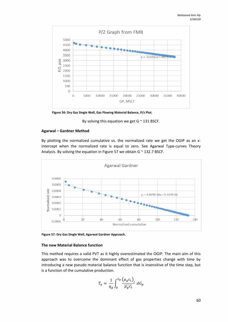
Mohamed Amr Aly

S236320

61

Figure 56: Dry Gas Single Well, Gas Flowing Material Balance, P/z Plot.

By solving this equation we get G ~ 131 BSCF.

Agarwal – Gardner Method

By plotting the normalized cumulative vs. the normalized rate we get the OGIP as an x-

intercept when the normalized rate is equal to zero. See Agarwal Type-curves Theory

Analysis. By solving the equation in Figure 57 we obtain G ~ 132.7 BSCF.

The new Material Balance function

This method requires a valid PVT as it highly overestimated the OGIP. The main aim of this

approach was to overcome the dominant effect of gas properties change with time by

introducing a new pseudo material balance function that is insensitive of the time step, but

is a function of the cumulative production.

𝑇𝑎 = 1

𝑞𝑔∫

(𝜇𝑔𝑐𝑡)𝑖𝜇𝑔̅̅ ̅𝑐�̅�

𝐺𝑝

0

𝑑𝐺𝑝

Figure 57: Dry Gas Single Well, Agarwal Gardner Approach.

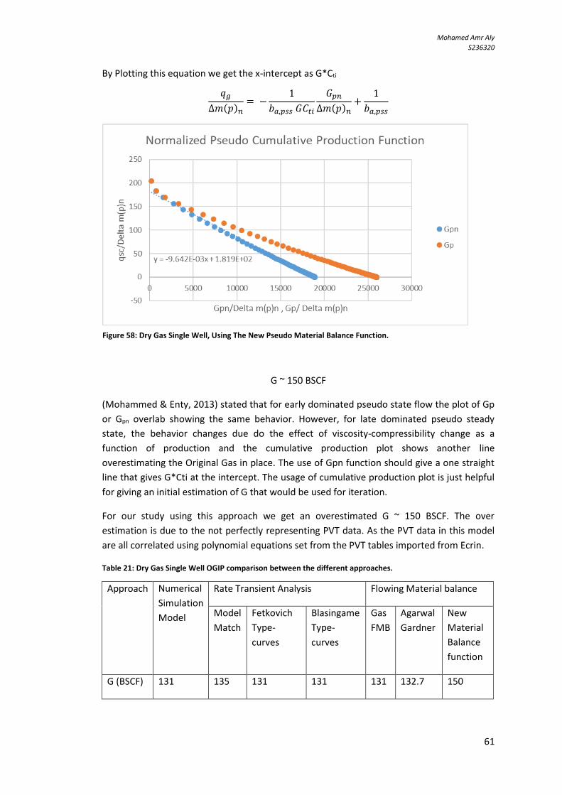
Mohamed Amr Aly

S236320

61

By Plotting this equation we get the x-intercept as G*Cti

𝑞𝑔

∆𝑚(𝑝)𝑛= −

1

𝑏𝑎,𝑝𝑠𝑠 𝐺𝐶𝑡𝑖


+1

𝑏𝑎,𝑝𝑠𝑠

G ~ 150 BSCF

(Mohammed & Enty, 2013) stated that for early dominated pseudo state flow the plot of Gp

or Gpn overlab showing the same behavior. However, for late dominated pseudo steady

state, the behavior changes due do the effect of viscosity-compressibility change as a

function of production and the cumulative production plot shows another line

overestimating the Original Gas in place. The use of Gpn function should give a one straight

line that gives G*Cti at the intercept. The usage of cumulative production plot is just helpful

for giving an initial estimation of G that would be used for iteration.

For our study using this approach we get an overestimated G ~ 150 BSCF. The over

estimation is due to the not perfectly representing PVT data. As the PVT data in this model

are all correlated using polynomial equations set from the PVT tables imported from Ecrin.

Table 21: Dry Gas Single Well OGIP comparison between the different approaches.

Approach Numerical

Simulation

Model

Rate Transient Analysis Flowing Material balance

Model

Match

Fetkovich

Type-

curves

Blasingame

Type-

curves

Gas

FMB

Agarwal

Gardner

New

Material

Balance

function

G (BSCF) 131 135 131 131 131 132.7 150

Figure 58: Dry Gas Single Well, Using The New Pseudo Material Balance Function.

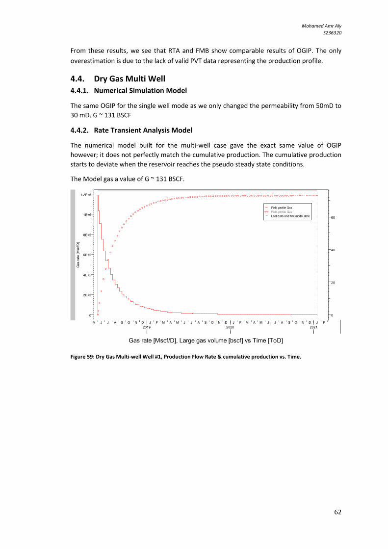
Mohamed Amr Aly

S236320

62

From these results, we see that RTA and FMB show comparable results of OGIP. The only

overestimation is due to the lack of valid PVT data representing the production profile.

4.4. Dry Gas Multi Well Numerical Simulation Model

The same OGIP for the single well mode as we only changed the permeability from 50mD to

30 mD. G ~ 131 BSCF


The numerical model built for the multi-well case gave the exact same value of OGIP

however; it does not perfectly match the cumulative production. The cumulative production

starts to deviate when the reservoir reaches the pseudo steady state conditions.

The Model gas a value of G ~ 131 BSCF.

Figure 59: Dry Gas Multi-well Well #1, Production Flow Rate & cumulative production vs. Time.

0

2E+5

4E+5

6E+5

8E+5

1E+6

1.2E+6

Gas

rate

[Msc

f/D]

0

20

40

60

Larg

e ga

s vo

lum

e [b

scf]

Field profile Gas

Field profile Gas

Last data and first model date

Prod

uctio

n [M

scf/D

]

M J J A S O N D J F M A M J J A S O N D2019

J F M A M J J A S O N D2020

J F2021

Gas rate [Mscf/D], Large gas volume [bscf] vs Time [ToD]

Mohamed Amr Aly

S236320

63

Well #1

Model Match

Figure 60: Dry Gas Multi-well Well #1 History Match. Rate, Cumulative production, flowing pressure and model

reservoir average pressure vs. Time.

Figure 61: Dry Gas Multi-well Well #1 Log-Log Plot Match.

0

1E+5

2E+5

3E+5

4E+5

Gas

rate

[Msc

f/D]

0

5E+9

1E+10

1.5E+10

Gas

vol

ume

[scf

]

q

Q

q model

Q model

0 2000 4000 6000 8000 10000 12000 14000 16000 18000 20000 22000 24000

Time [hr]

2500

3500

Pres

sure

[psi

a] Pi

p

Pbar


1E-6 1E-5 1E-4 1E-3 0.01 0.1 1 10 100 1000 10000 1E+5 1E+6 1E+7 1E+8Time [hr]

10

100

1000

10000

1E+5

1E+6

1E+7

1E+8

1E+9

Gas

pot

entia

l [ps

i2/c

p]




Well Vertical



Tmin 0 hr

Tmax 23040 hr

Total Skin 0


k, average 30 md

Pi 4500 psia

STGIIP 131 bscf

STGIP 113 bscf

Qg(tmax) 18.1 bscf

Skin 0

Skin 0

Skin 0

Skin 0

Pi 4500 psia

k.h 2400 md.ft

k 30 md

TMatch 28300 [hr]-1

PMatch 8.23E-4 [psi2/ cp]-1


Ab. time (ta) N/ A

Q(ta) N/ A


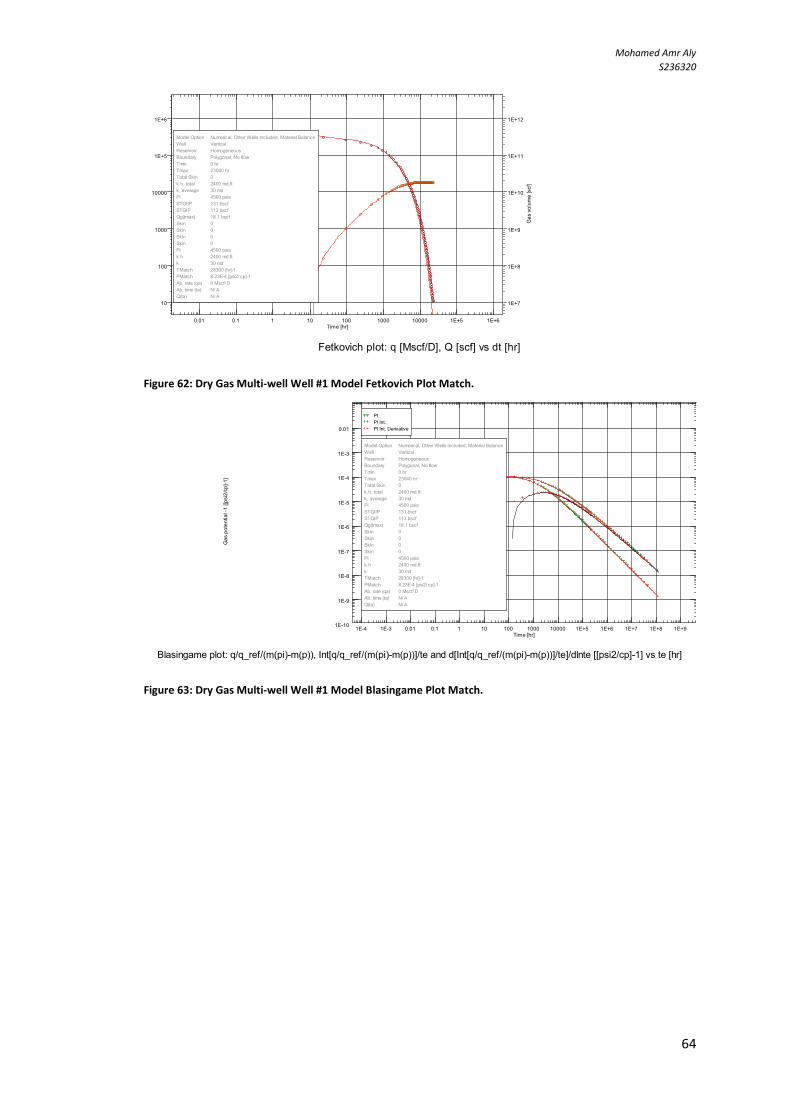
Mohamed Amr Aly

S236320

64

Figure 62: Dry Gas Multi-well Well #1 Model Fetkovich Plot Match.

Figure 63: Dry Gas Multi-well Well #1 Model Blasingame Plot Match.

0.01 0.1 1 10 100 1000 10000 1E+5 1E+6Time [hr]

10

100

1000

10000

1E+5

1E+6

Gas

rate

[Msc

f/D]

1E+7

1E+8

1E+9

1E+10

1E+11

1E+12

Gas

vol

ume

[scf

]


Well Vertical



Tmin 0 hr

Tmax 23040 hr

Total Skin 0


k, average 30 md

Pi 4500 psia

STGIIP 131 bscf

STGIP 113 bscf

Qg(tmax) 18.1 bscf

Skin 0

Skin 0

Skin 0

Skin 0

Pi 4500 psia

k.h 2400 md.ft

k 30 md

TMatch 28300 [hr]-1



Ab. time (ta) N/ A

Q(ta) N/ A


1E-4 1E-3 0.01 0.1 1 10 100 1000 10000 1E+5 1E+6 1E+7 1E+8 1E+9Time [hr]

1E-10

1E-9

1E-8

1E-7

1E-6

1E-5

1E-4

1E-3

0.01

Gas

pot

entia

l -1

[[psi

2/cp

]-1]

PI

PI Int.

PI Int. Derivative


Well Vertical



Tmin 0 hr

Tmax 23040 hr

Total Skin 0


k, average 30 md

Pi 4500 psia

STGIIP 131 bscf

STGIP 113 bscf

Qg(tmax) 18.1 bscf

Skin 0

Skin 0

Skin 0

Skin 0

Pi 4500 psia

k.h 2400 md.ft

k 30 md

TMatch 28300 [hr]-1



Ab. time (ta) N/ A

Q(ta) N/ A


Mohamed Amr Aly

S236320

65

Fetkovich Type-curves

Figure 64: Dry Gas Multi-well Well #1 Fetkovich Type-curves Match.

From Fetkovich Type-curves match, we can have an estimation of the Gas in place in the

drainage area covered by well #1

G1 ~ 32.6 BSCF


Figure 65: Dry Gas Multi-well Well #1 Blasingame Type-curves Match.

From Blasingame Type-curves match we obtain G1 ~33 BSCF

1E-6 1E-5 1E-4 1E-3 0.01 0.1 1 10 100 1000Not a unit

1E-5

1E-4

1E-3

0.01

0.1

1

10

100

Not

a u

nit

Re/ rwa=10

Re/ rwa=20

Re/ rwa=50

Re/ rwa=100

Re/ rwa=200

Re/ rwa=1000

Re/ rwa=10000

Re/ rwa=100000

exp(-tDd)

b=0

b=0.1

b=0.2

b=0.3

b=0.4

b=0.5

b=0.6

b=0.7

b=0.8

b=0.9

b=1

b 0.4

Di 0.0252 [Day]-1

qi 3E+5 Mscf/ D

UR 19.8 bscf

pwf 2000 psia

k.h 2740 md.ft

k 34.3 md

Re 1850 ft

rwa 0.36 ft

Skin 0.617

PV 30.5 MMB

STGIIP 32.6 bscf

STGIP 14.5 bscf


1E-5 1E-4 1E-3 0.01 0.1 1 10 100 1000 10000Not a unit

1E-4

1E-3

0.01

0.1

1

10

Not

a u

nit

Re/ rwa=4

Re/ rwa=12

Re/ rwa=28

Re/ rwa=80

Re/ rwa=160

Re/ rwa=800

Re/ rwa=2785.43

Re/ rwa=10000

qDd

qDdi

qDdid

STGIIP 33 bscf

STGIP 14.9 bscf

Re 1860 ft

rwa 0.542 ft

k.h 2540 md.ft

k 31.8 md

Skin 0.207


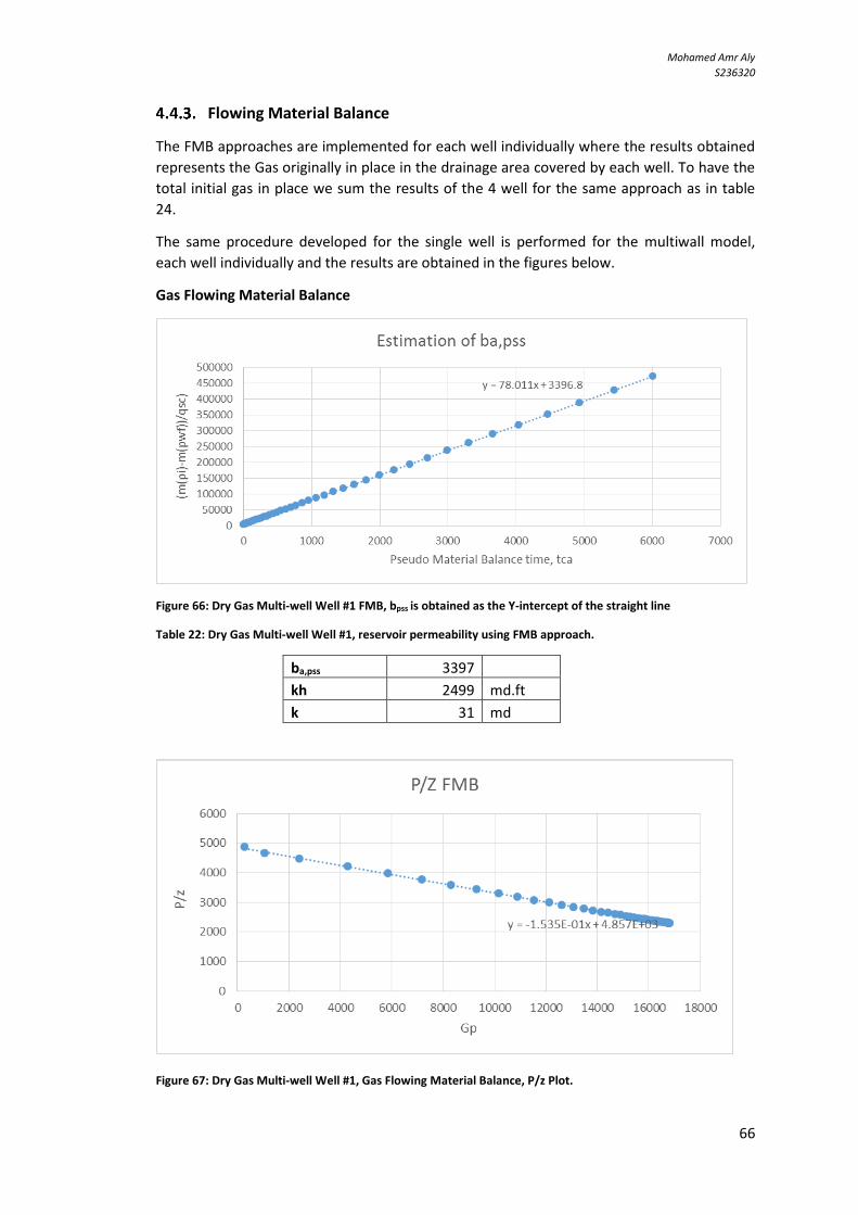
Mohamed Amr Aly

S236320

66


The FMB approaches are implemented for each well individually where the results obtained

represents the Gas originally in place in the drainage area covered by each well. To have the

total initial gas in place we sum the results of the 4 well for the same approach as in table

24.

The same procedure developed for the single well is performed for the multiwall model,

each well individually and the results are obtained in the figures below.


Figure 66: Dry Gas Multi-well Well #1 FMB, bpss is obtained as the Y-intercept of the straight line

Table 22: Dry Gas Multi-well Well #1, reservoir permeability using FMB approach.

ba,pss 3397

kh 2499 md.ft

k 31 md

Figure 67: Dry Gas Multi-well Well #1, Gas Flowing Material Balance, P/z Plot.

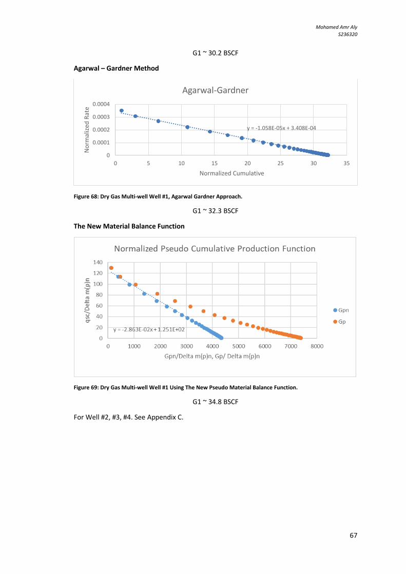
Mohamed Amr Aly

S236320

67

G1 ~ 30.2 BSCF

Agarwal – Gardner Method

Figure 68: Dry Gas Multi-well Well #1, Agarwal Gardner Approach.

G1 ~ 32.3 BSCF

The New Material Balance Function

Figure 69: Dry Gas Multi-well Well #1 Using The New Pseudo Material Balance Function.

G1 ~ 34.8 BSCF

For Well #2, #3, #4. See Appendix C.

y = -1.058E-05x + 3.408E-04

0

0.0001

0.0002

0.0003

0.0004

0 5 10 15 20 25 30 35

No

rmal

ized

Rat

e

Normalized Cumulative

Agarwal-Gardner

Mohamed Amr Aly

S236320

68

Table 23: Dry Gas Multi-well OGIP comparison between the different approaches.

Approach

Numerical

Simulation

Model

Rate Transient Analysis Flowing Material Balance

Model

Fetkovich

Type

Curves

Blasingame

Type

Curves

Gas

FMB

Agarwal-

Gardner

New

Material

Balance

Function

Well #1 - - 32.6 33 30.2 32.3 34.8

Well #2 - - 32.1 32.8 30.5 32.5 34.9

Well #3 - - 32.7 32.4 30.5 32.6 34.9

Well #4 - - 32.7 32.5 30.8 32.8 35.1

G (BSCF) 131 131 130.1 130.7 122 130 139.7

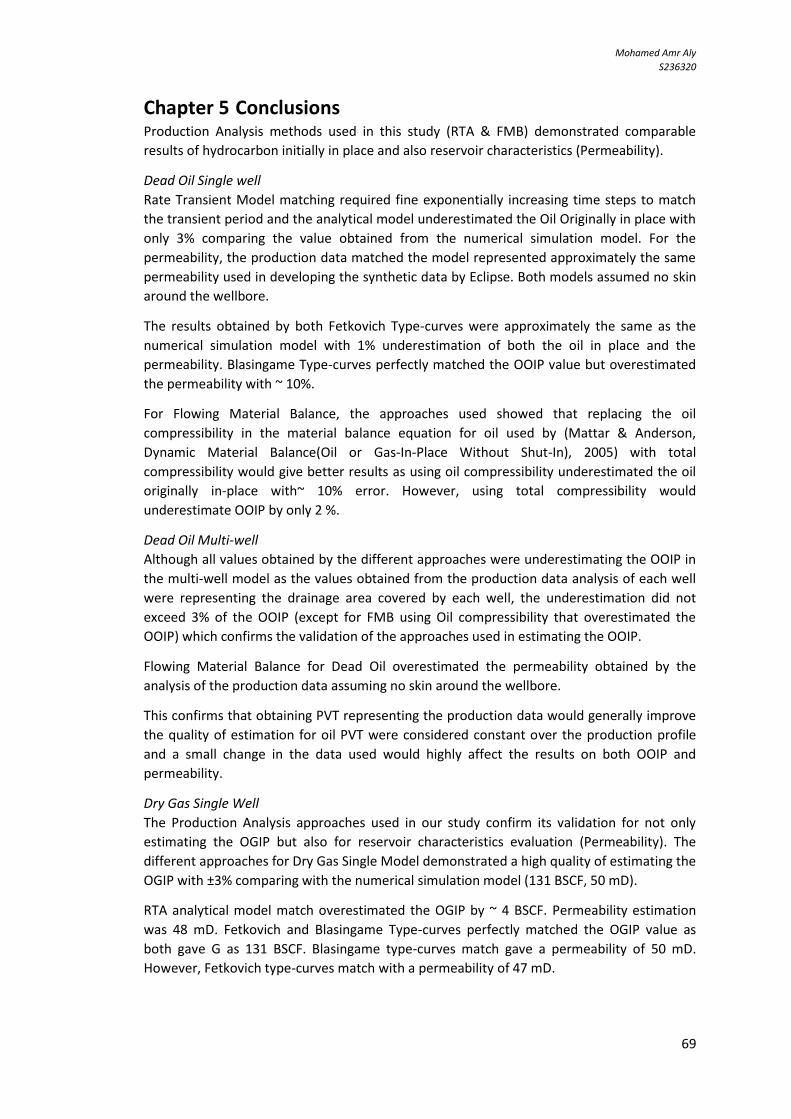
Mohamed Amr Aly

S236320

69

Chapter 5 Conclusions Production Analysis methods used in this study (RTA & FMB) demonstrated comparable

results of hydrocarbon initially in place and also reservoir characteristics (Permeability).

Dead Oil Single well

Rate Transient Model matching required fine exponentially increasing time steps to match

the transient period and the analytical model underestimated the Oil Originally in place with

only 3% comparing the value obtained from the numerical simulation model. For the

permeability, the production data matched the model represented approximately the same

permeability used in developing the synthetic data by Eclipse. Both models assumed no skin

around the wellbore.

The results obtained by both Fetkovich Type-curves were approximately the same as the

numerical simulation model with 1% underestimation of both the oil in place and the

permeability. Blasingame Type-curves perfectly matched the OOIP value but overestimated

the permeability with ~ 10%.

For Flowing Material Balance, the approaches used showed that replacing the oil

compressibility in the material balance equation for oil used by (Mattar & Anderson,

Dynamic Material Balance(Oil or Gas-In-Place Without Shut-In), 2005) with total

compressibility would give better results as using oil compressibility underestimated the oil

originally in-place with~ 10% error. However, using total compressibility would

underestimate OOIP by only 2 %.

Dead Oil Multi-well

Although all values obtained by the different approaches were underestimating the OOIP in

the multi-well model as the values obtained from the production data analysis of each well

were representing the drainage area covered by each well, the underestimation did not

exceed 3% of the OOIP (except for FMB using Oil compressibility that overestimated the

OOIP) which confirms the validation of the approaches used in estimating the OOIP.

Flowing Material Balance for Dead Oil overestimated the permeability obtained by the

analysis of the production data assuming no skin around the wellbore.

This confirms that obtaining PVT representing the production data would generally improve

the quality of estimation for oil PVT were considered constant over the production profile

and a small change in the data used would highly affect the results on both OOIP and

permeability.

Dry Gas Single Well

The Production Analysis approaches used in our study confirm its validation for not only

estimating the OGIP but also for reservoir characteristics evaluation (Permeability). The

different approaches for Dry Gas Single Model demonstrated a high quality of estimating the

OGIP with ±3% comparing with the numerical simulation model (131 BSCF, 50 mD).

RTA analytical model match overestimated the OGIP by ~ 4 BSCF. Permeability estimation

was 48 mD. Fetkovich and Blasingame Type-curves perfectly matched the OGIP value as

both gave G as 131 BSCF. Blasingame type-curves match gave a permeability of 50 mD.

However, Fetkovich type-curves match with a permeability of 47 mD.

Mohamed Amr Aly

S236320

71

Flowing Material Balance approaches used in this study strongly confirmed its validation as

the new method of estimating OGIP using production data. The newly introduced iterative

method gave comparable results from the second iterative step.

For Gas FMB and Agarwal – Gardner approaches, both required to iterate the assumed value

of G in two steps to reach the representing value of G for the single well model. However,

the results did not confirm what demonstrated in study of (Ismadi, Kabir, & Hasan, 2012)

based on comparing the two approaches. They showed that Agarwal – Gardner approach

should give more accurate results than the Gas FMB approach as evaluating the average

pressure in the first approach (Agarwal – Gardner) depends on the conventional MBE.

However in the later (Gas FMB), the evaluation uses the fluid flow equation after estimating

the pseudo-steady state constant bpss. In our study, we observed that Gas FMB perfectly

gave the OGIP value estimated by the numerical simulation model and Agarwal – Gardner

method overestimated the value. Nevertheless, the difference is less than 1 % of the

numerical simulation model.

On the other hand, using the new material balance function introduced by (Mohammed &

Enty, 2013) and was confirmed later by (Molokwu & Onyekonwu, 2016) highly

overestimated the OGIP value.

The reason of this unexpected overestimation could be due to the quality of the PVT data

generated for this approach. The calculation of the normalized pseudo cumulative function

depends on the viscosity compressibility ratio values at the representing cumulative

production values. This is developed by fitting a polynomial equation that showed a

considerable error that could be clearly seen in Figure 29 as the first value of the viscosity

compressibility should be equal to 1. This error because of the consecutive usage of

polynomial equations of for generating compressibility and viscosity values from the PVT

data imported from Ecrin.

Dry Gas Multi-Well

The match of the numerical model of RTA on Topaze, Fetkovich type-curve and Blasingame

type-curves gave the value of Gas in place in the drainage areas covered by the wells and the

summation of these values gave a strong agreement with the OGIP value estimated by the

numerical simulation model.

For Flowing Material Balance approaches, the contrary of what was experienced in the

single well model happened. The Agarwal – Gardner approach showed its validation for

estimating OGIP over the FMB approach using material balance time. Although the

normalized pseudo cumulative function showed its equivalence with the material balance

time function or it is even better as it is not sensitive to the time step and the gas properties

change is considered as a function of the cumulative production, not as a function of time,

the application of the new material balance approach using the normalized pseudo

cumulative function still overestimated the OGIP and again this is a result of the PVT data.

To sum up, Production Data Analysis approaches could give reliable results for the

estimation of the initial hydrocarbon in place and the reservoir characteristics. Flowing

Material Balance is a valid approach for estimating the Original Hydrocarbon in Place. PVT

data surveillance during production is crucial for production analysis in general and for FMB

in specific.

Mohamed Amr Aly

S236320

71

Bibliography and References Agarwal, R. G., Gardner, D. C., Kleinsteiber, S. W., & Fussell, D. D. (1998). Analyzing Well

Production Data Using Combined Type Curve and Decline Curve Analysis Concepts. .

Ahmed, T. (2010). Reservoir engineering handbook, Fourth edition. Elsvier.

Arps , J. J. (1945). Analysis of Decline Curves. . Society of Petroleum Engineers.

Aziz , K., & Settari , A. (1979). Petroleum Reservoir Simulation . In Petroleum Reservoir

Simulation . Amesterdam: Elsevier Applied Science Publisher .

Callard, J. G., & Schenewerk, P. A. (1995). Reservoir Performance History Matching Using

Rate/Cumulative Type-Curves. Society of Petroleum Engineers.

Choudhury, Z., & Gomes, E. (2000). Material Balance Study of Gas Reservoirs by Flowing Well

Method: A Case Study of Bakhrabad Gas Field. Society of Petroleum Engineers.

Dake, L. (n.d.). Fundamentals of Reservoir Engineering. The Netherlands: Shell Internationale

Petroleum Maatschappij B. V.The Hague.

Damoah, L. O., Mohammed, S., & Enty, G. S. (2015). Utilizing early time boundary-dominated

flow data to make an initial estimate of gas-in-place: An aid to computing material

balance pseudotime. Society of Petroleum Engineers .

DIATI, P. (2018). Reservoir Engineering Lectures. Turin.

Elgmati , A. R. (2015). Analysis of production and pressure data to characterize the

performance of oil and gas reservoir. Society of Petroleum Engineers .

Fekete.com. (n.d.). Agarwal-Gardner Theory. Retrieved June 3, 2018, from

http://www.fekete.com/SAN/WebHelp/FeketeHarmony/Harmony_WebHelp/Conte

nt/HTML_Files/Reference_Material/Analysis_Method_Theory/Agarwal-

Gardner_Theory.htm

Fekete.com. (n.d.). Blasingame Theory. Retrieved June 5, 2018, from


nt/HTML_Files/Reference_Material/Analysis_Method_Theory/Blasingame_Theory.h

tm

Fekete.com. (n.d.). Fetkovich Theory. Retrieved June 2, 2018, from


nt/HTML_Files/Reference_Material/Analysis_Method_Theory/Fetkovich_Theory.ht

m

Fekete.com. (n.d.). Flowing Material Balance Theory. Retrieved June 30, 2018, from

http://fekete.com/SAN/TheoryAndEquations/HarmonyTheoryEquations/Content/HT

ML_Files/Reference_Material/Analysis_Method_Theory/FMB_Theory.htm

Fekete.com. (n.d.). Material Balance Time Theory. Retrieved May 30, 2018, from


nt/HTML_Files/Reference_Material/General_Concepts/Material_Balance_Time_The

ory.htm

Mohamed Amr Aly

S236320

72

Fekete.com. (n.d.). Traditional Decline Theory. Retrieved June 25, 2018, from


nt/HTML_Files/Reference_Material/Analysis_Method_Theory/Traditional_Decline_T

heory.htm

Fetkovich, M. J. (1980). Decline curve analysis using type curves. Society of Petroleum

Engineers.

Guzman, J. D., Arevalo, J. A., & Espinola, O. (2014). Reserves evaluation of dry gas reservoirs

through flowing pressure material balance method. Society of Petroleum Engineers .

Harold Vance Department of Petroleum Engineering. (n.d.). Introduction to Petroleum

Engineering. Texas A&M University.

Institute of Petroleum Engineering, . (n.d.). Reservoir Simulation Book. United Kingdom:

Heriot-Watt University.

Ismadi, D., Kabir, C. S., & Hasan, R. (2012). The use of combined static- and dynamic-

material-balance methods with real-time surveillance data in volumetric gas

reservoirs. Society of Petroleum Engineers.

Istayeva, U., & King, G. (2014). Application of the extended dynamic material balance

method to a super-giant carbonate oilfield. Society of Petroleum Engineers.

Ltd., S. (2014). Eclipse Reference Manual Version 2014.1. Schlumberger Ltd.

Mattar , L., & Anderson, D. (2005). Dynamic Material Balance(Oil or Gas-In-Place Without

Shut-In). Petroleum Society of Canada.

Mattar , L., & McNeil, R. (1998). The "Flowing" Gas Maerial Balance . Petroleum Society of

Canada .

McNeil, R. (1995). The "Flowing" Material Balance Procedure. Petroleum Society of Canda.

Meunier, D. F., Kabir, C. S., & Wittmann, M. J. (1987). Gas Well Test Analysis: Use of

Normalized Pseudovariables. Society of Petroleum Engineers.

Mohammed, S., & Enty, G. S. (2013). Analysis of Gas Production Data Using Flowing Material

Balance Method. Society of Petroleum Engineers .

Molokwu, V. C., & Onyekonwu, M. O. (2016). A Nonlinear Flowing Material Balance for

Analysis of Gas Well Production Data. Society of Petroleum Engineers.

Morad , K., & Clarkson, C. R. (2006). Application of Flowing P/z* Material Balance for Dry

Coalbed-Methane Reservoirs . Society of Petroleum Engineers .

Nnaemeka, E. (2011). Petroleum Reservoir Engineering Practice . USA .

Ojo, K. P., & Osisanya, S. O. (2006). Material Balance Revisited. Sociey of Petroleum

Engineers.

Ojo, K. P., Tiab, D., & Osisanya, S. O. (2006). Dynamic Material Balance Equation and Solution

Technique Using Production and PVT Data. Society of Petroleum Engineers .

Mohamed Amr Aly

S236320

73

Oliver, H., Didier , V., Ole, S. F., & et al. (2013). The theory and practice of pressure transient,

Production analysis, Well performance analysis, Production logging and the use of

permanent downhole gauge data. KAPPA V.4.20.2015.

Palacio, J. C., & Blasingame, T. A. (1993). Decline-Curve Analysis With Type Curves - Analysis

of Gas Well Production Data. Society of Petroleum Engineers .

Ukauku, I., Johnson, A., Olatunji, B., Korubo, W., Olugbenga, D., Nwashinemere, U., &

Iledare, W. (2017). Flowing material balance and rate transient analysis modeling

with augmented non-continuous permanent downhole gauge data. Society of

Petroleum Engineers .

Van Everdingen, A. F., & Hurst, W. (1949). The Application of the Laplace Transformation to

Flow Problems in Reservoirs. Society of Petroleum Engineers .

Mohamed Amr Aly

S236320

74

Appendix A Fluid Flow Equations in Porous medium for different flow regimes (DIATI, 2018)

In this part we develop the derivation of the fluid flow equations that would be further used

in the FMB approaches.

We start from the solution to the diffusivity equation. The diffusivity equation is a

differential equation obtained by combining continuity equation that governs the

conservation of mass, flaw law and state equations. It's a Partial differential equation that

describes the change of the pressure in space in time in the reservoir.

Assuming Monophasic flow of a slightly compressible fluid (Liquid) through a homogeneous

and Isotropic porous medium, pressure gradients are small and Darcy's law applies we

reach:

∇2𝑝 = 𝜇𝜙𝑐𝑡𝑘

𝜕𝑝

𝜕𝑡= 1

𝜂

𝜕𝑝

𝜕𝑡 Equation A-1

Where 𝜂 is defined as Diffusivity constant

𝜂 =𝑘

𝜇𝜙𝑐𝑡 Equation A-2

Developing the equation for radial flow we reach:

Steady State Flow

𝜕2𝑝

𝜕𝑟2+1

𝑟

𝜕𝑝

𝜕𝑟= 0 Equation A-3

Defining the initial and boundary conditions: {𝜕𝑝

𝜕𝑡= 0 ∀𝑟, ∀𝑡

𝑝 = 𝑝𝑖 = 𝑐𝑜𝑛𝑠𝑡. 𝑟 = 𝑟𝑒

Solving the diffusivity equation we get MUSKAT Equation where

𝑞 = 2 𝜋𝑘ℎ

𝜇 𝑝𝑖 − 𝑝𝑤

ln𝑟𝑒𝑟𝑤

Equation A-4

which also can be written as:

𝑝𝑤𝑓 = 𝑝𝑖 −𝑞 𝜇

2 𝜋𝑘ℎ ln

𝑟𝑒𝑟𝑤

Equation A-5

Introducing the skin factor we reach

𝑝𝑤𝑓 = 𝑝𝑖 −𝑞 𝜇

2 𝜋𝑘ℎ ln (

𝑟𝑒𝑟𝑤+ 𝑆) Equation A-6

Knowing that this in the SI units we can get this equation in Oil-field units as:

𝑝𝑤𝑓 = 𝑝𝑖 −141.27 𝑞 𝐵𝜇

𝑘ℎ ln (

𝑟𝑒𝑟𝑤+ 𝑆) Equation A-7

Mohamed Amr Aly

S236320

75

Where,

p (psi)

q (STB/d)

𝜇 (cP)

K (mD)

h (ft)

re, rw (ft)

B (bbl/STB) , S (-)

Transient Flow

𝜕2𝑝

𝜕𝑟2+1

𝑟

𝜕𝑝

𝜕𝑟= 𝜇𝜙𝑐𝑡𝑘

𝜕𝑝


Initial and boundary conditions:

{

𝑡 = 𝑜, 𝑝 = 𝑝𝑖 ∀𝑟

𝑡 > 0 {𝑝 = 𝑝𝑖 𝑟 = 𝑟𝑒

𝜕𝑝

𝜕𝑟= 𝑐𝑜𝑛𝑠𝑡𝑎𝑛𝑡 𝑟 = 𝑟𝑤

𝐶𝑜𝑛𝑠𝑡𝑎𝑛𝑡 𝑇𝑒𝑟𝑚𝑖𝑛𝑎𝑙 𝑅𝑎𝑡𝑒

Solving the diffusivity equation we reach

𝑝(𝑟𝑤, 𝑡) = 𝑝𝑖 −𝑞 𝜇

2 𝜋𝑘ℎ 𝑃 (

𝑟

𝑟𝑤, 𝑡𝐷) Equation A-9

Before we proceed, we would like to define what is called dimensionless variables.

Dimensionless Variables have been used in well testing to solve the unsteady-state flow

equation and to simply the diffusivity equation and its solution. Hence, reduce the number

of unknowns by combining the reservoir parameters (Such as permeability, Porosity).

(Ahmed, 2010)

Dimensionless Pressure Variable PD:

𝑃𝐷 = 2 𝜋 𝑘 ℎ

𝑞 𝜇∆𝑝 Equation A-10

In the oil field units:

𝑃𝐷 = 𝑘ℎ

141.27 𝑞 𝐵 𝜇 ∆𝑝 =

0.007082 𝑘ℎ

𝑞 𝐵 𝜇 ∆𝑝 Equation A-11

Dimensionless Time Variable tD:

𝑡𝐷 =𝑡

𝑡𝑐=

𝑘𝑡

𝜇𝜙𝑐𝑡𝑟𝑤2

Equation A-12

Mohamed Amr Aly

S236320

76

Where tc is the characteristic time:

(𝑡)𝑐 =𝜇𝜙𝑐𝑡𝑟𝑤

2

𝑘 Equation A-13

In the oil field units:

𝑡𝐷 =𝑡

(𝑡)𝑐=0.0002637 𝑘𝑡


Equation A-14

Dimensionless Outer Boundary Radius Variable reD:

𝑟𝑒𝐷 =𝑟𝑒𝑟𝑤

Equation A-15

Dimensionless Radius Variable rD:

𝑟𝑒𝐷 =𝑟𝑒𝑟𝑤

Equation A-16

Back to the solution of the diffusivity equation, the solution of the term 𝑃 (𝑟

𝑟𝑤, 𝑡𝐷) was

found in literature as:

𝑃 (𝑟

𝑟𝑤, 𝑡𝐷) = −

1

2𝐸𝑖 (−

𝑟2

4 𝜂𝑡 ) Equation A-17

Where,

𝐸𝑖 (−𝑟2

4 𝜂𝑡 ) = ln (

4

𝑒𝛾𝑡𝐷) = ln(2.25 𝑡𝐷) = ln(2.25


𝑘𝑡 )

Equation A-18

Where 𝛾 = 0.57721 is defined as Euler's Constant

Therefore, 𝑝 (𝑟𝑤 , 𝑡) = 𝑝𝑖 −𝑞 𝜇

2 𝜋𝑘ℎ (−

1

2ln(2.25


𝑘𝑡 )) Equation A-19

𝑝 (𝑟𝑤, 𝑡) = 𝑝𝑖 −𝑞 𝜇

4 𝜋𝑘ℎ ln (2.25

𝑘𝑡

𝜇𝜙𝑐𝑡𝑟𝑤2 ) = 𝑝𝑖 −

𝑞 𝜇

4 𝜋𝑘ℎ ln(2.25𝑡𝐷) Equation A-20

Introducing the skin factor


4 𝜋𝑘ℎ ln (2.25

𝑘𝑡

𝜇𝜙𝑐𝑡𝑟𝑤2+ 2𝑆 ) Equation A-21

𝑝 (𝑟𝑤 , 𝑡) = 𝑝𝑖 −𝑞 𝜇

4 𝜋𝑘ℎ ln(2.25𝑡𝐷 + 2𝑆 ) Equation A-22

Mohamed Amr Aly

S236320

77

In the Oil-Field Units

𝑝 (𝑟𝑤 , 𝑡) = 𝑝𝑖 −70.64 𝑞 𝐵 𝜇

𝑘ℎ ln (2.25

𝑘𝑡

𝜇𝜙𝑐𝑡𝑟𝑤2+ 2𝑆 ) Equation A-23

𝑝 (𝑟𝑤, 𝑡) = 𝑝𝑖 −70.64 𝑞 𝐵 𝜇

𝑘ℎ ln(2.25𝑡𝐷 + 2𝑆 ) Equation A-24

Pseudo-Steady State Flow

𝜕2𝑝

𝜕𝑟2+1

𝑟

𝜕𝑝

𝜕𝑟= 𝜇𝜙𝑐𝑡𝑘

𝜕𝑝


Initial and boundary conditions:

{

𝑡 = 𝑜, 𝑝 = 𝑝𝑖 𝑟 = 𝑟𝑒

𝑡 > 0 {

𝑑𝑝

𝑑𝑡= 𝑐𝑜𝑛𝑠𝑡 ∀ 𝑟

𝜕𝑝

𝜕𝑟= 0 𝑟 = 𝑟𝑒

A Pseudo-Steady State condition is reached when all boundaries of the reservoir is touched

and the reservoir is acting as enclosed system where the pressure starts to drop with the

same rate at each point in the reservoir.

From the flow equation of the transient flow, we can define the time to reach the pseudo-

steady state (Stabilization time) as:

𝑡𝑠 =1

2.25

𝜇𝜙𝑐𝑡𝑟𝑒2

𝑘 Equation A-26

However, the reservoir boundaries rarely take a regular shape and therefore the well is

probably asymmetrically located in a bounded, irregularly shaped drainage area which

makes the flow equations we have developed in a porous medium are no longer valid

because of the additional pressure drop of due to the reflection of the pressure disturbances

on the boundaries.

Applying the superposition in space and assuming a linear boundary we get:


2 𝜋𝑘ℎ (1

2ln(2.25𝑡𝐷) + 𝑃 (

𝑑

𝑟𝑤, 𝑡𝐷)) Equation A-27

As d is the distance between the well and the boundary at which the pressure disturbance

will reflect. Therefore,

𝑃 (𝑑

𝑟𝑤, 𝑡𝐷) = −

1

2𝐸𝑖 (−

𝑑2

4 𝜂𝑡 ) Equation A-28

Mohamed Amr Aly

S236320

78

However, the well could be affected by the reflections of infinite number of boundaries each

according to the distance from the well and therefore:


4 𝜋𝑘ℎ [ln 2.25𝑡𝐷 − ∑𝐸𝑖 (−

𝑑𝑗2

4 𝜂𝑡 )

∞

𝑗=1

] Equation A-29

To solve this newly introduced term we introduce another dimensionless variable.

Dimensionless time Variable with respect to the drainage are tDA:

𝑡𝐷𝐴 = 𝑘𝑡

𝜇𝜙𝑐𝑡𝐴= 𝑡𝐷

𝑟𝑤2

𝐴 Equation A-30

In addition (Matthews, Brons, Hazeborek) introduced a function called MBH or F function

that depends on {𝑇𝑖𝑚𝑒

𝑆ℎ𝑎𝑝𝑒 𝑜𝑓 𝑡ℎ𝑒 𝐷𝑟𝑎𝑖𝑛𝑎𝑔𝑒 𝑎𝑟𝑒𝑎 𝑊𝑒𝑙𝑙 𝐿𝑜𝑐𝑎𝑡𝑖𝑜𝑛

that will be used to solve this term where:

𝐹 = 4 𝜋 𝑡𝐷𝐴 + ∑𝐸𝑖 (−𝑑𝑗2

4 𝜂𝑡 )

∞

𝑗=1

Equation A-31

This gives us the general flow equation that is also used in late transient flow to address the

influence of the boundaries of the drainage as:


4 𝜋𝑘ℎ [ln 2.25𝑡𝐷 + 4 𝜋 𝑡𝐷𝐴 − 𝐹 ] Equation A-32

When Pseudo-Steady State (PSS) it's found that F function stabilizes and becomes linear

𝐹 = ln𝐶𝐴𝑡𝐷𝐴 Equation A-33

Where CA is defined as Dietz Shape Factor that depends on the shape of the drainage are and

on the well location within it.


4 𝜋𝑘ℎ [ln 2.25𝑡𝐷 + 4 𝜋 𝑡𝐷𝐴 − 𝐹 ] Equation A-34


4 𝜋𝑘ℎ [ln 2.25𝑡𝐷 + 4 𝜋 𝑡𝐷𝐴 − ln𝐶𝐴𝑡𝐷𝐴 ] Equation A-35


4 𝜋𝑘ℎ [ln 2.25

𝐴

𝐶𝐴𝑟𝑤2+ 4 𝜋 𝑡𝐷𝐴 ] Equation A-36

In the meanwhile, if the reservoir conditions reached PSS this means that depletion started

to occur. Depletion energy is completely driven by the compressibility of the fluid in the

pores of the reservoir roc and from the definition of the compressibility:

𝑐 =1

𝑉

∆𝑉

∆𝑃 Equation A-37

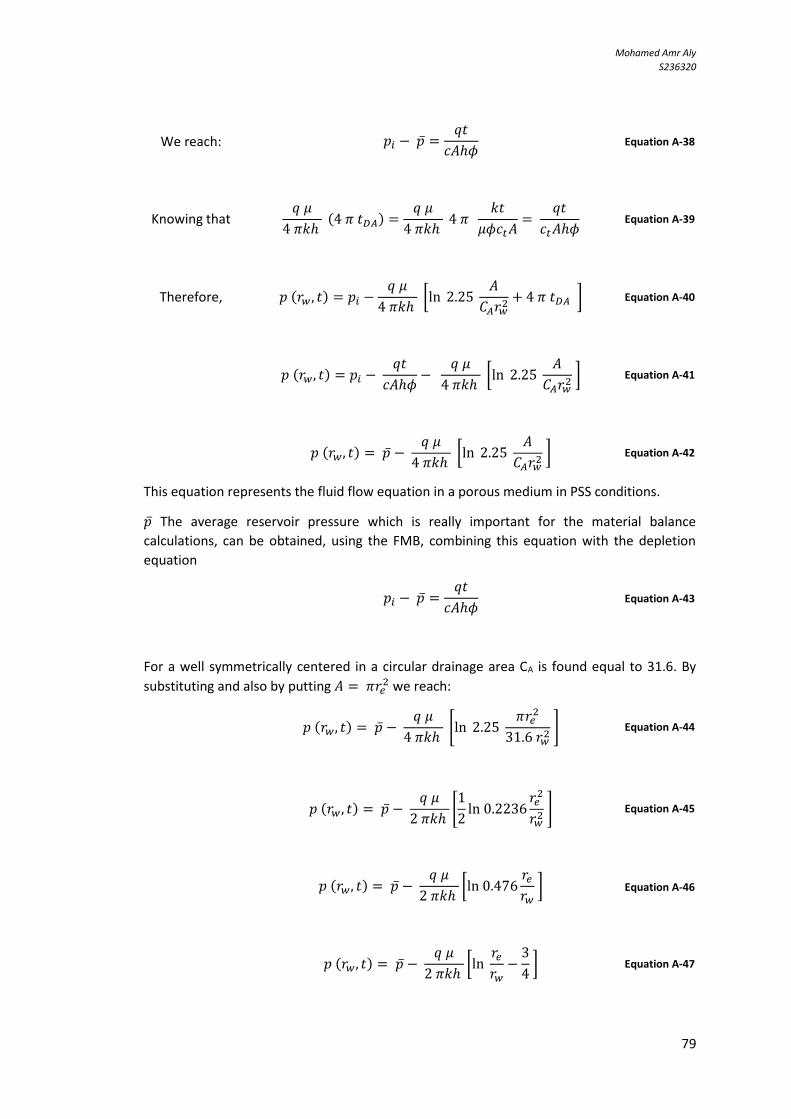
Mohamed Amr Aly

S236320

79

We reach: 𝑝𝑖 − �̅� =𝑞𝑡

𝑐𝐴ℎ𝜙 Equation A-38

Knowing that 𝑞 𝜇

4 𝜋𝑘ℎ (4 𝜋 𝑡𝐷𝐴) =

𝑞 𝜇

4 𝜋𝑘ℎ 4 𝜋

𝑘𝑡

𝜇𝜙𝑐𝑡𝐴=

𝑞𝑡

𝑐𝑡𝐴ℎ𝜙 Equation A-39

Therefore, 𝑝 (𝑟𝑤 , 𝑡) = 𝑝𝑖 −𝑞 𝜇

4 𝜋𝑘ℎ [ln 2.25

𝐴


𝑝 (𝑟𝑤, 𝑡) = 𝑝𝑖 − 𝑞𝑡

𝑐𝐴ℎ𝜙−

𝑞 𝜇

4 𝜋𝑘ℎ [ln 2.25

𝐴

𝐶𝐴𝑟𝑤2 ] Equation A-41

𝑝 (𝑟𝑤, 𝑡) = �̅� − 𝑞 𝜇

4 𝜋𝑘ℎ [ln 2.25

𝐴


This equation represents the fluid flow equation in a porous medium in PSS conditions.

�̅� The average reservoir pressure which is really important for the material balance

calculations, can be obtained, using the FMB, combining this equation with the depletion

equation

𝑝𝑖 − �̅� =𝑞𝑡

𝑐𝐴ℎ𝜙 Equation A-43

For a well symmetrically centered in a circular drainage area CA is found equal to 31.6. By

substituting and also by putting 𝐴 = 𝜋𝑟𝑒2 we reach:

𝑝 (𝑟𝑤, 𝑡) = �̅� − 𝑞 𝜇

4 𝜋𝑘ℎ [ln 2.25

𝜋𝑟𝑒2

31.6 𝑟𝑤2 ] Equation A-44

𝑝 (𝑟𝑤 , 𝑡) = �̅� − 𝑞 𝜇

2 𝜋𝑘ℎ [1

2ln 0.2236

𝑟𝑒2

𝑟𝑤2 ] Equation A-45

𝑝 (𝑟𝑤, 𝑡) = �̅� − 𝑞 𝜇

2 𝜋𝑘ℎ [ln 0.476

𝑟𝑒𝑟𝑤 ] Equation A-46

𝑝 (𝑟𝑤, 𝑡) = �̅� − 𝑞 𝜇

2 𝜋𝑘ℎ [ln

𝑟𝑒𝑟𝑤−3

4 ] Equation A-47

Mohamed Amr Aly

S236320

81

This is the liquid flow equation in a porous medium in a PSS conditions for an asymmetrically

centered well in a circular drainage area.

Liquid Flow Equations:

1) General equation: This equation is used in late transient conditions.

𝑝𝑤𝑓 = 𝑝𝑖 −𝑞𝑜 𝜇𝑜4 𝜋𝑘ℎ

[ln 2.25𝑡𝐷 + 4 𝜋 𝑡𝐷𝐴 − 𝐹 + 2𝑆 ] Equation A-48

2) Early Transient conditions (where no boundary is felt) and in RTA is called Infinite

Acting Radial Flow

𝑝𝑤𝑓 = 𝑝𝑖 −𝑞𝑜 𝜇𝑜4 𝜋𝑘ℎ

ln(2.25𝑡𝐷 + 2𝑆 ) Equation A-49

3) Pseudo-Steady State Conditions:

𝑝𝑤𝑓 = �̅� − 𝑞𝑜 𝜇𝑜4 𝜋𝑘ℎ

[ln 2.25 𝐴


Gas Flow Equations:

Instead of derivation all equations again for the gas, we use the dimensionless terms.

Recall the dimensionless pressure variable Equation A-10:

∆𝑝 = 𝑞 𝜇

2 𝜋 𝑘 ℎ 𝑃𝐷 = 𝑝𝑖 − 𝑝(𝑟𝑤 , 𝑡) Equation A-51

Therefore we could express the dimensionless pressure variable according to the flow

regime

General Equation (Always Valid)

𝑃𝐷 = 1

2 [ln 2.25𝑡𝐷 + 4 𝜋 𝑡𝐷𝐴 − 𝐹] Equation A-52

Early Transient Conditions

𝑃𝐷 =1

2 ln(2.25𝑡𝐷 ) Equation A-53

Pseudo-Steady State Conditions

𝑃𝐷 =1

2[ln 2.25

𝐴


Pseudo Steady State conditions (Well symmetrically centered in a circular drainage

area)

𝑃𝐷 = 2𝜋𝑡𝐷𝐴 + [ln 𝑟𝑒

𝑟𝑤−3

4 ] Equation A-55

Mohamed Amr Aly

S236320

81

This found in literature expressed as:

𝑃𝐷 = 2 𝑡𝐷

𝑟𝑒𝐷2 + ln(𝑟𝑒𝐷) −

3

4 Equation A-56

Using these equations gives the same equations with only two changes:

The Pseudo Pressure Function instead of the Pressure to account for the change of

compressibility factor Z and viscosity of the gas with the change of pressure.

In literature, the pseudo-pressure function could be found expressed as:

𝑚(𝑝) = 2∫𝑝

𝑍𝜇𝑑𝑝

𝑝

𝑝𝑜

Equation A-57

The proportionality in the dimensionless parameters equation

For Liquid Flow equation we found in Equation A-10

∆𝑝 = 𝑞 𝜇

2 𝜋 𝑘 ℎ 𝑃𝐷

However, for gas flow equations with introducing the pseudo pressure function to have the

rigorous solution of the diffusivity equation, it is found that:

∆𝑚(𝑝) = 𝑞𝑔 𝑇

𝜋 𝑘 ℎ (𝑃𝑠𝑐𝑇𝑠𝑐) 𝑃𝐷 Equation A-58

1) General equation: This equation is used in late transient conditions.

𝑚(𝑝𝑤𝑓) = 𝑚(𝑝𝑖) −𝑞𝑔 𝑇

2𝜋 𝑘 ℎ (𝑃𝑠𝑐𝑇𝑠𝑐) [ln 2.25𝑡𝐷 + 4 𝜋 𝑡𝐷𝐴 − 𝐹 + 2𝑆 ] Equation A-59

2) Early Transient conditions (where no boundary is felt) and in RTA is called Infinite

Acting Radial Flow

𝑚(𝑝𝑤𝑓 ) = 𝑚(𝑝𝑖) −𝑞𝑔 𝑇

2𝜋 𝑘 ℎ (𝑃𝑠𝑐𝑇𝑠𝑐) ln(2.25𝑡𝐷 + 2𝑆 ) Equation A-60

3) Pseudo-Steady State Conditions:

𝑚(𝑝𝑤𝑓) = 𝑚(�̅�) −𝑞𝑔 𝑇


𝐴


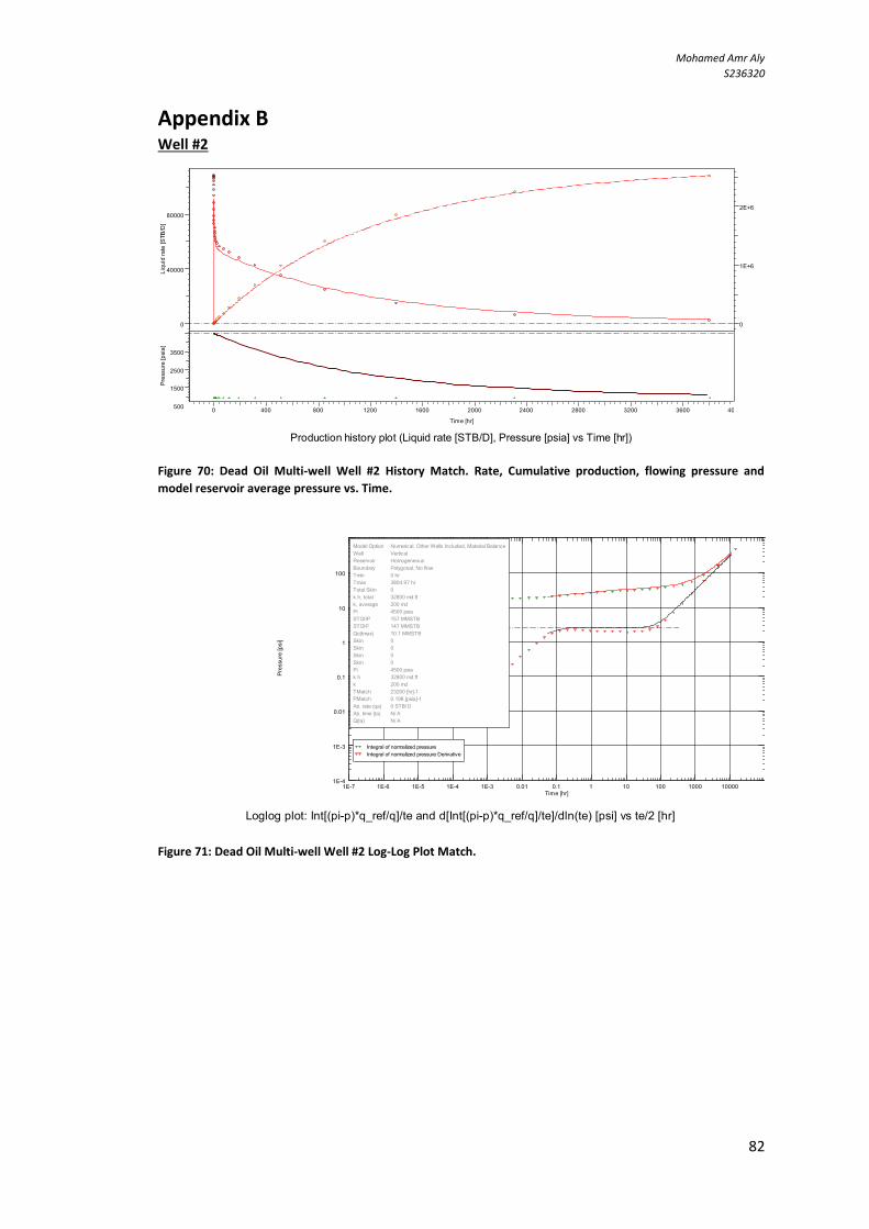
Mohamed Amr Aly

S236320

82

Appendix B Well #2



Figure 71: Dead Oil Multi-well Well #2 Log-Log Plot Match.

0

40000

80000

Liqu

id ra

te [S

TB/D

]

0

1E+6

2E+6

Liqu

id v

olum

e [S

TB]

0 400 800 1200 1600 2000 2400 2800 3200 3600 4000

Time [hr]

500

1500

2500

3500

Pres

sure

[psi

a]


1E-7 1E-6 1E-5 1E-4 1E-3 0.01 0.1 1 10 100 1000 10000Time [hr]

1E-4

1E-3

0.01

0.1

1

10

100

Pres

sure

[psi

]




Well Vertical



Tmin 0 hr

Tmax 3804.97 hr

Total Skin 0


k, average 200 md

Pi 4500 psia

STOIIP 157 MMSTB

STOIP 147 MMSTB

Qo(tmax) 10.1 MMSTB

Skin 0

Skin 0

Skin 0

Skin 0

Pi 4500 psia

k.h 32800 md.ft

k 200 md

TMatch 23200 [hr]-1



Ab. time (ta) N/ A

Q(ta) N/ A


Mohamed Amr Aly

S236320

83



1E-6 1E-5 1E-4 1E-3 0.01 0.1 1 10 100 1000 10000Time [hr]

1E-5

1E-4

1E-3

0.01

0.1

Pres

sure

-1 [[

psi]-

1]

PI

PI Int.

PI Int. Derivative


Well Vertical



Tmin 0 hr

Tmax 3804.97 hr

Total Skin 0


k, average 200 md

Pi 4500 psia

STOIIP 157 MMSTB

STOIP 147 MMSTB

Qo(tmax) 10.1 MMSTB

Skin 0

Skin 0

Skin 0

Skin 0

Pi 4500 psia

k.h 32800 md.ft

k 200 md

TMatch 23200 [hr]-1



Ab. time (ta) N/ A

Q(ta) N/ A


1E-8 1E-7 1E-6 1E-5 1E-4 1E-3 0.01 0.1 1 10 100 1000 10000Time [hr]

10

100

1000

10000

1E+5

1E+6

1E+7

Liqu

id ra

te [S

TB/D

]

1

10

100

1000

10000

1E+5

1E+6

Liqu

id v

olum

e [S

TB]


Well Vertical



Tmin 0 hr

Tmax 3804.97 hr

Total Skin 0


k, average 200 md

Pi 4500 psia

STOIIP 157 MMSTB

STOIP 147 MMSTB

Qo(tmax) 10.1 MMSTB

Skin 0

Skin 0

Skin 0

Skin 0

Pi 4500 psia

k.h 32800 md.ft

k 200 md

TMatch 23200 [hr]-1



Ab. time (ta) N/ A

Q(ta) N/ A


Mohamed Amr Aly

S236320

84







The match of the Blasingame type-curve give an estimation of the OOIP stored in the

drainage area covered by each well. For Well #2 it gives ~ 39.2 MMSTB

1E-4 1E-3 0.01 0.1 1 10Not a unit

1E-3

0.01

0.1

1

Not

a u

nit

Re/ rwa=10

Re/ rwa=20

Re/ rwa=50

Re/ rwa=100

Re/ rwa=200

Re/ rwa=1000

Re/ rwa=10000

Re/ rwa=100000

exp(-tDd)

b=0

b=0.1

b=0.2

b=0.3

b=0.4

b=0.5

b=0.6

b=0.7

b=0.8

b=0.9

b=1

b 0

Di 0.0206 [Day]-1

qi 55200 STB/ D

UR 2.67 MMSTB

pwf 900 psia

k.h 36200 md.ft

k 221 md

Re 1850 ft

rwa 0.483 ft

Skin 0.323

PV 62.8 MMB

STOIIP 39.2 MMSTB

STOIP 29.1 MMSTB


1E-4 1E-3 0.01 0.1 1 10 100Not a unit

0.01

0.1

1

10

Not

a u

nit

Re/ rwa=4

Re/ rwa=12

Re/ rwa=28

Re/ rwa=80

Re/ rwa=160

Re/ rwa=800

Re/ rwa=2772.54

Re/ rwa=10000

qDd

qDdi

qDdid

STOIIP 39.2 MMSTB

STOIP 29.1 MMSTB

Re 1850 ft

rwa 0.449 ft

k.h 38600 md.ft

k 235 md

Skin 0.396


Mohamed Amr Aly

S236320

85




Kh 44123.43 mD.ft

k 269.0 mD




𝑞 vs

𝑁𝑝


1




Figure 76: Dead Oil Multi-well Well #2 FMB, bpss is obtained as the Y-intercept of the straight

line.

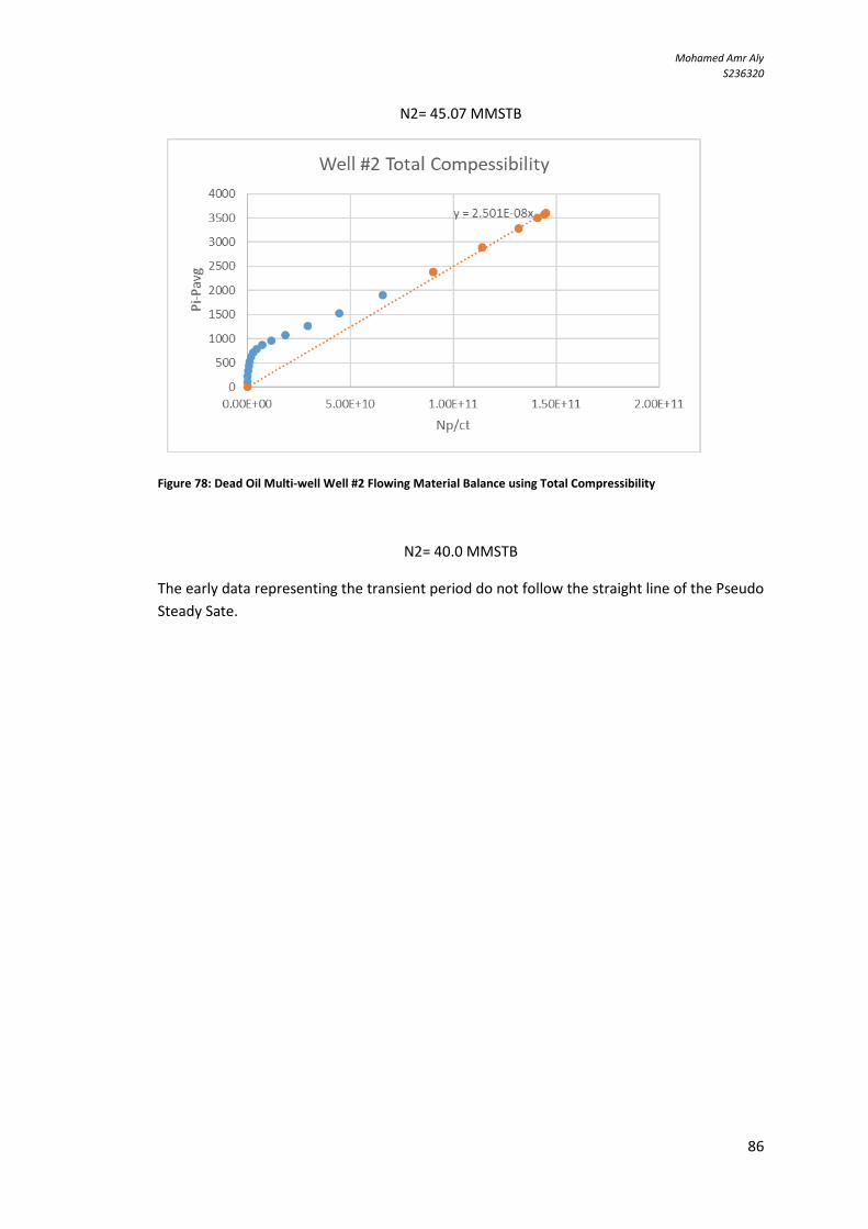
Mohamed Amr Aly

S236320

86

N2= 45.07 MMSTB

Figure 78: Dead Oil Multi-well Well #2 Flowing Material Balance using Total Compressibility

N2= 40.0 MMSTB

The early data representing the transient period do not follow the straight line of the Pseudo

Steady Sate.

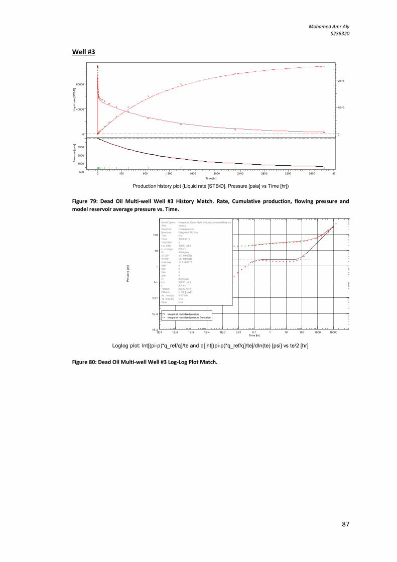
Mohamed Amr Aly

S236320

87

Well #3




0

40000

80000

Liqu

id ra

te [S

TB/D

]

0

1E+6

2E+6

Liqu

id v

olum

e [S

TB]

0 400 800 1200 1600 2000 2400 2800 3200 3600 4000

Time [hr]

500

1500

2500

3500

Pres

sure

[psi

a]


1E-7 1E-6 1E-5 1E-4 1E-3 0.01 0.1 1 10 100 1000 10000Time [hr]

1E-4

1E-3

0.01

0.1

1

10

100

Pres

sure

[psi

]




Well Vertical



Tmin 0 hr

Tmax 3804.97 hr

Total Skin 0


k, average 200 md

Pi 4500 psia

STOIIP 157 MMSTB

STOIP 147 MMSTB

Qo(tmax) 10.1 MMSTB

Skin 0

Skin 0

Skin 0

Skin 0

Pi 4500 psia

k.h 32800 md.ft

k 200 md

TMatch 23200 [hr]-1



Ab. time (ta) N/ A

Q(ta) N/ A


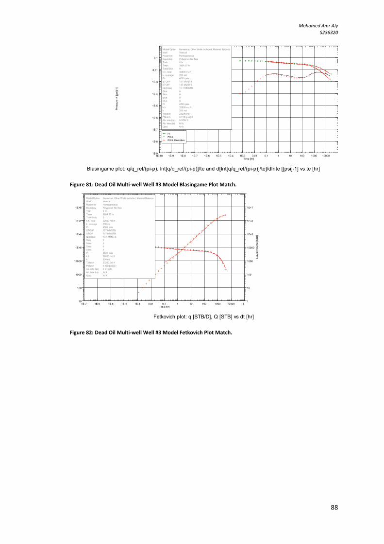
Mohamed Amr Aly

S236320

88



1E-10 1E-9 1E-8 1E-7 1E-6 1E-5 1E-4 1E-3 0.01 0.1 1 10 100 1000 10000Time [hr]

1E-9

1E-8

1E-7

1E-6

1E-5

1E-4

1E-3

0.01

0.1

Pres

sure

-1 [[

psi]-

1]

PI

PI Int.

PI Int. Derivative


Well Vertical



Tmin 0 hr

Tmax 3804.97 hr

Total Skin 0


k, average 200 md

Pi 4500 psia

STOIIP 157 MMSTB

STOIP 147 MMSTB

Qo(tmax) 10.1 MMSTB

Skin 0

Skin 0

Skin 0

Skin 0

Pi 4500 psia

k.h 32800 md.ft

k 200 md

TMatch 23200 [hr]-1



Ab. time (ta) N/ A

Q(ta) N/ A


1E-7 1E-6 1E-5 1E-4 1E-3 0.01 0.1 1 10 100 1000 10000 1E+5Time [hr]

10

100

1000

10000

1E+5

1E+6

1E+7

1E+8

Liqu

id ra

te [S

TB/D

]

1

10

100

1000

10000

1E+5

1E+6

1E+7

Liqu

id v

olum

e [S

TB]


Well Vertical



Tmin 0 hr

Tmax 3804.97 hr

Total Skin 0


k, average 200 md

Pi 4500 psia

STOIIP 157 MMSTB

STOIP 147 MMSTB

Qo(tmax) 10.1 MMSTB

Skin 0

Skin 0

Skin 0

Skin 0

Pi 4500 psia

k.h 32800 md.ft

k 200 md

TMatch 23200 [hr]-1



Ab. time (ta) N/ A

Q(ta) N/ A


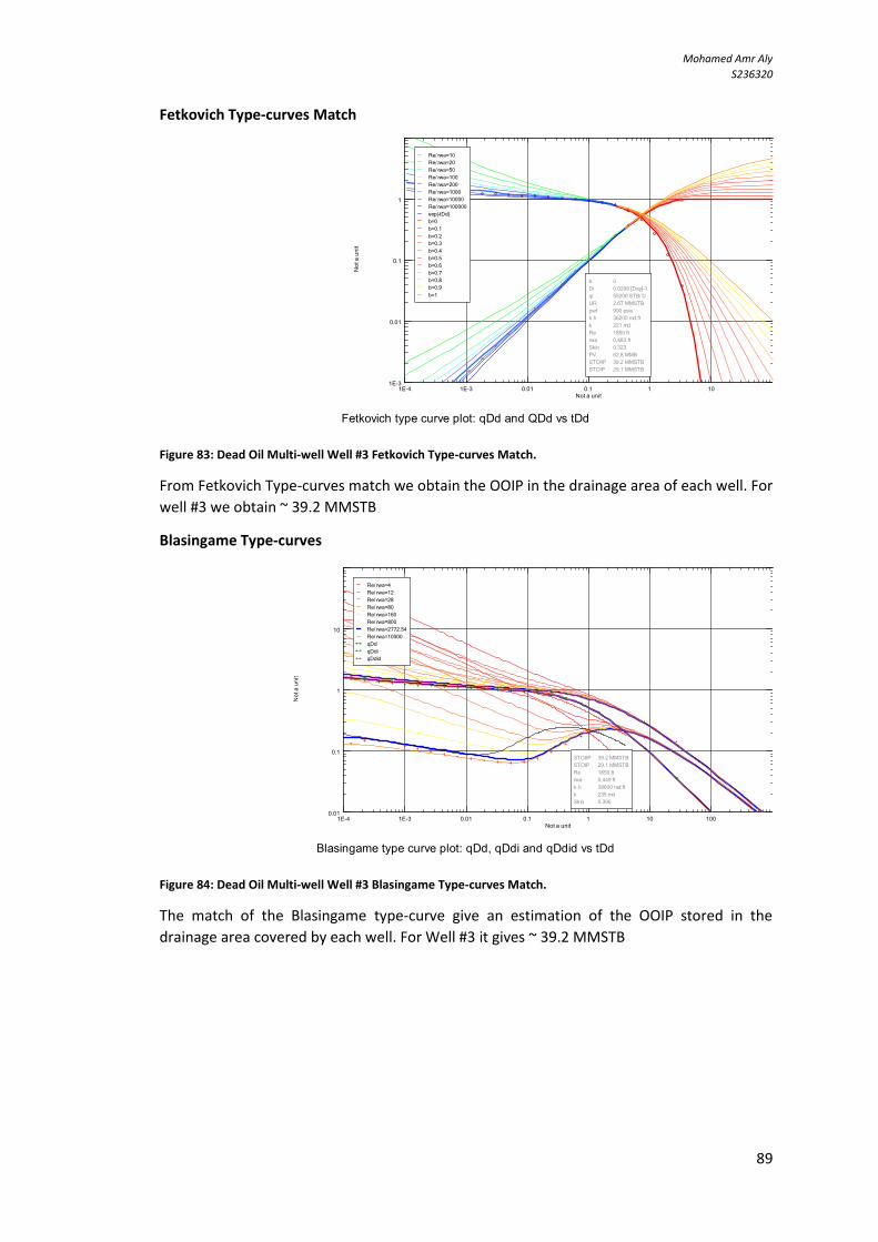
Mohamed Amr Aly

S236320

89









1E-4 1E-3 0.01 0.1 1 10Not a unit

1E-3

0.01

0.1

1

Not

a u

nit

Re/ rwa=10

Re/ rwa=20

Re/ rwa=50

Re/ rwa=100

Re/ rwa=200

Re/ rwa=1000

Re/ rwa=10000

Re/ rwa=100000

exp(-tDd)

b=0

b=0.1

b=0.2

b=0.3

b=0.4

b=0.5

b=0.6

b=0.7

b=0.8

b=0.9

b=1

b 0

Di 0.0206 [Day]-1

qi 55200 STB/ D

UR 2.67 MMSTB

pwf 900 psia

k.h 36200 md.ft

k 221 md

Re 1850 ft

rwa 0.483 ft

Skin 0.323

PV 62.8 MMB

STOIIP 39.2 MMSTB

STOIP 29.1 MMSTB


1E-4 1E-3 0.01 0.1 1 10 100Not a unit

0.01

0.1

1

10

Not

a u

nit

Re/ rwa=4

Re/ rwa=12

Re/ rwa=28

Re/ rwa=80

Re/ rwa=160

Re/ rwa=800

Re/ rwa=2772.54

Re/ rwa=10000

qDd

qDdi

qDdid

STOIIP 39.2 MMSTB

STOIP 29.1 MMSTB

Re 1850 ft

rwa 0.449 ft

k.h 38600 md.ft

k 235 md

Skin 0.396


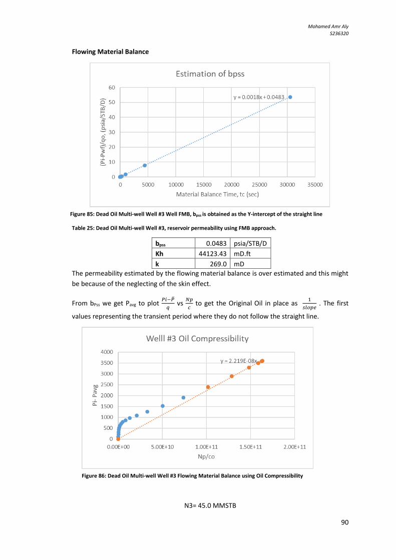
Mohamed Amr Aly

S236320

91

Figure 85: Dead Oil Multi-well Well #3 Well FMB, bpss is obtained as the Y-intercept of the straight line





Kh 44123.43 mD.ft

k 269.0 mD




𝑞 vs

𝑁𝑝


1



N3= 45.0 MMSTB

Mohamed Amr Aly

S236320

91


N3 = 40.0 MMSTB


Steady Sate.

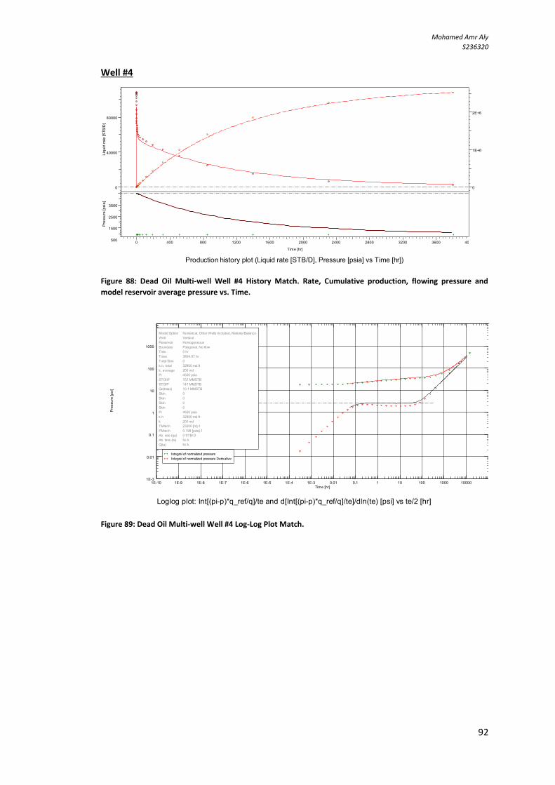
Mohamed Amr Aly

S236320

92

Well #4




0

40000

80000

Liqu

id ra

te [S

TB/D

]

0

1E+6

2E+6

Liqu

id v

olum

e [S

TB]

0 400 800 1200 1600 2000 2400 2800 3200 3600 4000

Time [hr]

500

1500

2500

3500

Pres

sure

[psi

a]


1E-10 1E-9 1E-8 1E-7 1E-6 1E-5 1E-4 1E-3 0.01 0.1 1 10 100 1000 10000Time [hr]

1E-3

0.01

0.1

1

10

100

1000

Pres

sure

[psi

]




Well Vertical



Tmin 0 hr

Tmax 3804.97 hr

Total Skin 0


k, average 200 md

Pi 4500 psia

STOIIP 157 MMSTB

STOIP 147 MMSTB

Qo(tmax) 10.1 MMSTB

Skin 0

Skin 0

Skin 0

Skin 0

Pi 4500 psia

k.h 32800 md.ft

k 200 md

TMatch 23200 [hr]-1



Ab. time (ta) N/ A

Q(ta) N/ A


Mohamed Amr Aly

S236320

93


Figure 91: Dead Oil Multi-well Well #4 Well Model Fetkovich Plot Match.

1E-7 1E-6 1E-5 1E-4 1E-3 0.01 0.1 1 10 100 1000 10000Time [hr]

1E-5

1E-4

1E-3

0.01

0.1

Pres

sure

-1 [[

psi]-

1]

PI

PI Int.

PI Int. Derivative


Well Vertical



Tmin 0 hr

Tmax 3804.97 hr

Total Skin 0


k, average 200 md

Pi 4500 psia

STOIIP 157 MMSTB

STOIP 147 MMSTB

Qo(tmax) 10.1 MMSTB

Skin 0

Skin 0

Skin 0

Skin 0

Pi 4500 psia

k.h 32800 md.ft

k 200 md

TMatch 23200 [hr]-1



Ab. time (ta) N/ A

Q(ta) N/ A


1E-6 1E-5 1E-4 1E-3 0.01 0.1 1 10 100 1000 10000Time [hr]

10

100

1000

10000

1E+5

1E+6

1E+7

Liqu

id ra

te [S

TB/D

]

1

10

100

1000

10000

1E+5

1E+6

Liqu

id v

olum

e [S

TB]


Well Vertical



Tmin 0 hr

Tmax 3804.97 hr

Total Skin 0


k, average 200 md

Pi 4500 psia

STOIIP 157 MMSTB

STOIP 147 MMSTB

Qo(tmax) 10.1 MMSTB

Skin 0

Skin 0

Skin 0

Skin 0

Pi 4500 psia

k.h 32800 md.ft

k 200 md

TMatch 23200 [hr]-1



Ab. time (ta) N/ A

Q(ta) N/ A


Mohamed Amr Aly

S236320

94









1E-4 1E-3 0.01 0.1 1 10Not a unit

1E-3

0.01

0.1

1

Not

a u

nit

Re/ rwa=10

Re/ rwa=20

Re/ rwa=50

Re/ rwa=100

Re/ rwa=200

Re/ rwa=1000

Re/ rwa=10000

Re/ rwa=100000

exp(-tDd)

b=0

b=0.1

b=0.2

b=0.3

b=0.4

b=0.5

b=0.6

b=0.7

b=0.8

b=0.9

b=1

b 0

Di 0.021 [Day]-1

qi 56200 STB/ D

UR 2.67 MMSTB

pwf 900 psia

k.h 36900 md.ft

k 225 md

Re 1850 ft

rwa 0.483 ft

Skin 0.323

PV 62.8 MMB

STOIIP 39.2 MMSTB

STOIP 29.1 MMSTB


1E-4 1E-3 0.01 0.1 1 10 100Not a unit

0.01

0.1

1

10

Not

a u

nit

Re/ rwa=4

Re/ rwa=12

Re/ rwa=28

Re/ rwa=80

Re/ rwa=160

Re/ rwa=800

Re/ rwa=2772.54

Re/ rwa=10000

qDd

qDdi

qDdid

STOIIP 40.7 MMSTB

STOIP 30.6 MMSTB

Re 1880 ft

rwa 0.457 ft

k.h 38600 md.ft

k 235 md

Skin 0.378


Mohamed Amr Aly

S236320

95

Figure 94: Dead Oil Multi-well Well #4 FMB, bpss is obtained as the Y-intercept of the straight line.

Figure 95: Dead Oil Multi-well Well #4 Flowing Material Balance using Oil Compressibility.




Kh 44214.98 mD.ft

k 269.6 mD




𝑞 vs

𝑁𝑝


1



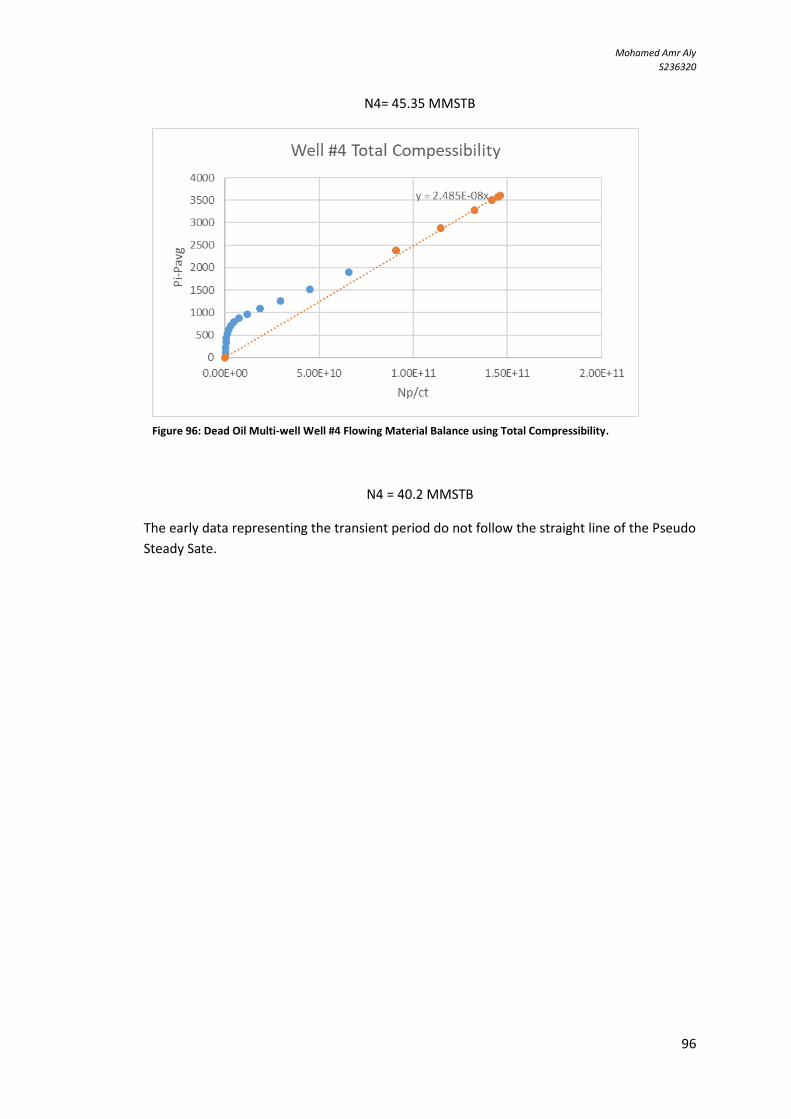
Mohamed Amr Aly

S236320

96


N4= 45.35 MMSTB

N4 = 40.2 MMSTB


Steady Sate.

Mohamed Amr Aly

S236320

97

Appendix C Dry Gas Multi-Well Results

Well #2

Model Match

Figure 97: Dry Gas Multi-well Well #2 History Match. Rate, Cumulative production, flowing pressure and model

reservoir average pressure vs. Time.


0

1E+5

2E+5

3E+5

4E+5

Gas

rate

[Msc

f/D]

0

1E+10

Gas

vol

ume

[scf

]

q

Q

q model

Q model

0 2000 4000 6000 8000 10000 12000 14000 16000 18000 20000 22000 24000

Time [hr]

2500

3500

Pres

sure

[psi

a] Pi

p

Pbar


1E-5 1E-4 1E-3 0.01 0.1 1 10 100 1000 10000 1E+5 1E+6 1E+7Time [hr]

10

100

1000

10000

1E+5

1E+6

1E+7

1E+8

Gas

pot

entia

l [ps

i2/c

p]


Well Vertical



Tmin 0 hr

Tmax 23040 hr

Total Skin 0


k, average 30 md

Pi 4500 psia

STGIIP 131 bscf

STGIP 113 bscf

Qg(tmax) 18.2 bscf

Skin 0

Skin 0

Skin 0

Skin 0

Pi 4500 psia

k.h 2400 md.ft

k 30 md

TMatch 28300 [hr]-1



Ab. time (ta) N/ A

Q(ta) N/ A


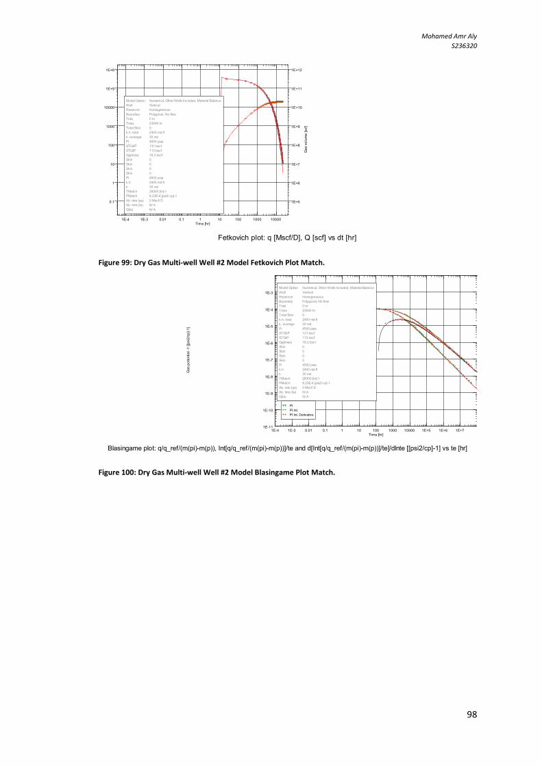
Mohamed Amr Aly

S236320

98



1E-4 1E-3 0.01 0.1 1 10 100 1000 10000Time [hr]

0.1

1

10

100

1000

10000

1E+5

1E+6

Gas

rate

[Msc

f/D]

1E+5

1E+6

1E+7

1E+8

1E+9

1E+10

1E+11

1E+12

Gas

vol

ume

[scf

]


Well Vertical



Tmin 0 hr

Tmax 23040 hr

Total Skin 0


k, average 30 md

Pi 4500 psia

STGIIP 131 bscf

STGIP 113 bscf

Qg(tmax) 18.2 bscf

Skin 0

Skin 0

Skin 0

Skin 0

Pi 4500 psia

k.h 2400 md.ft

k 30 md

TMatch 28300 [hr]-1



Ab. time (ta) N/ A

Q(ta) N/ A


1E-4 1E-3 0.01 0.1 1 10 100 1000 10000 1E+5 1E+6 1E+7Time [hr]

1E-11

1E-10

1E-9

1E-8

1E-7

1E-6

1E-5

1E-4

1E-3

Gas

pot

entia

l -1

[[psi

2/cp

]-1]

PI

PI Int.

PI Int. Derivative


Well Vertical



Tmin 0 hr

Tmax 23040 hr

Total Skin 0


k, average 30 md

Pi 4500 psia

STGIIP 131 bscf

STGIP 113 bscf

Qg(tmax) 18.2 bscf

Skin 0

Skin 0

Skin 0

Skin 0

Pi 4500 psia

k.h 2400 md.ft

k 30 md

TMatch 28300 [hr]-1



Ab. time (ta) N/ A

Q(ta) N/ A


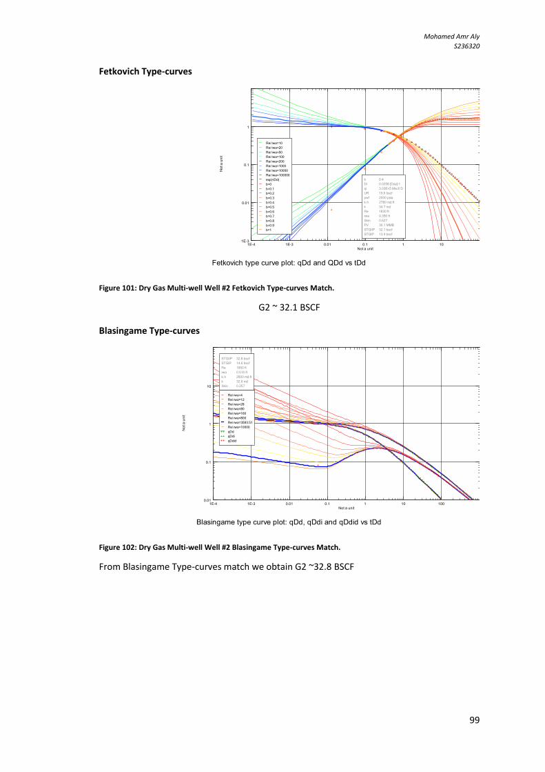
Mohamed Amr Aly

S236320

99



G2 ~ 32.1 BSCF



From Blasingame Type-curves match we obtain G2 ~32.8 BSCF

1E-4 1E-3 0.01 0.1 1 10Not a unit

1E-3

0.01

0.1

1

Not

a u

nit

Re/ rwa=10

Re/ rwa=20

Re/ rwa=50

Re/ rwa=100

Re/ rwa=200

Re/ rwa=1000

Re/ rwa=10000

Re/ rwa=100000

exp(-tDd)

b=0

b=0.1

b=0.2

b=0.3

b=0.4

b=0.5

b=0.6

b=0.7

b=0.8

b=0.9

b=1

b 0.4

Di 0.0258 [Day]-1

qi 3.03E+5 Mscf/ D

UR 19.6 bscf

pwf 2000 psia

k.h 2780 md.ft

k 34.7 md

Re 1830 ft

rwa 0.356 ft

Skin 0.627

PV 30.1 MMB

STGIIP 32.1 bscf

STGIP 13.9 bscf


1E-4 1E-3 0.01 0.1 1 10 100Not a unit

0.01

0.1

1

10

Not

a u

nit

Re/ rwa=4

Re/ rwa=12

Re/ rwa=28

Re/ rwa=80

Re/ rwa=160

Re/ rwa=800

Re/ rwa=3593.51

Re/ rwa=10000

qDd

qDdi

qDdid

STGIIP 32.8 bscf

STGIP 14.6 bscf

Re 1850 ft

rwa 0.515 ft

k.h 2600 md.ft

k 32.6 md

Skin 0.257


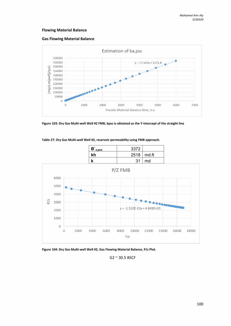
Mohamed Amr Aly

S236320

111





B`a,pss 3372 kh 2518 md.ft k 31 md


G2 ~ 30.5 BSCF

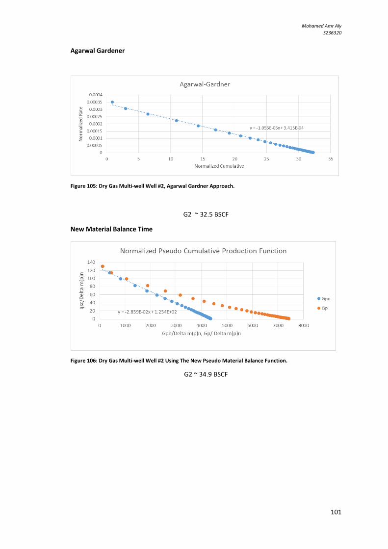
Mohamed Amr Aly

S236320

111

Agarwal Gardener


G2 ~ 32.5 BSCF

New Material Balance Time


G2 ~ 34.9 BSCF

Mohamed Amr Aly

S236320

112

Well #3

Model Match

Figure 107: Dry Gas Multi-well Well #3 History Match. Rate, Cumulative production, flowing pressure and



0

1E+5

2E+5

3E+5

4E+5

Gas

rate

[Msc

f/D]

0

1E+10

Gas

vol

ume

[scf

]

q

Q

q model

Q model

0 2000 4000 6000 8000 10000 12000 14000 16000 18000 20000 22000 24000

Time [hr]

2500

3500

Pres

sure

[psi

a] Pi

p

Pbar


1E-9 1E-8 1E-7 1E-6 1E-5 1E-4 1E-3 0.01 0.1 1 10 100 1000 100001E+5 1E+6 1E+7Time [hr]

1E-3

0.01

0.1

1

10

100

1000

10000

1E+5

1E+6

1E+7

1E+8

1E+9

1E+10

1E+11

Gas

pot

entia

l [ps

i2/c

p]




Well Vertical



Tmin 0 hr

Tmax 23040 hr

Total Skin 0


k, average 30 md

Pi 4500 psia

STGIIP 131 bscf

STGIP 113 bscf

Qg(tmax) 18.2 bscf

Skin 0

Skin 0

Skin 0

Skin 0

Pi 4500 psia

k.h 2400 md.ft

k 30 md

TMatch 28300 [hr]-1



Ab. time (ta) N/ A

Q(ta) N/ A


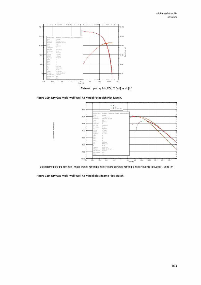
Mohamed Amr Aly

S236320

113



1E-3 0.01 0.1 1 10 100 1000 10000 1E+5Time [hr]

10

100

1000

10000

1E+5

1E+6

Gas

rate

[Msc

f/D]

1E+7

1E+8

1E+9

1E+10

1E+11

1E+12

Gas

vol

ume

[scf

]


Well Vertical



Tmin 0 hr

Tmax 23040 hr

Total Skin 0


k, average 30 md

Pi 4500 psia

STGIIP 131 bscf

STGIP 113 bscf

Qg(tmax) 18.2 bscf

Skin 0

Skin 0

Skin 0

Skin 0

Pi 4500 psia

k.h 2400 md.ft

k 30 md

TMatch 28300 [hr]-1



Ab. time (ta) N/ A

Q(ta) N/ A


1E-5 1E-4 1E-3 0.01 0.1 1 10 100 1000 10000 1E+5 1E+6 1E+7Time [hr]

1E-10

1E-9

1E-8

1E-7

1E-6

1E-5

1E-4

1E-3

Gas

pot

entia

l -1

[[psi

2/cp

]-1]

PI

PI Int.

PI Int. Derivative


Well Vertical



Tmin 0 hr

Tmax 23040 hr

Total Skin 0


k, average 30 md

Pi 4500 psia

STGIIP 131 bscf

STGIP 113 bscf

Qg(tmax) 18.2 bscf

Skin 0

Skin 0

Skin 0

Skin 0

Pi 4500 psia

k.h 2400 md.ft

k 30 md

TMatch 28300 [hr]-1



Ab. time (ta) N/ A

Q(ta) N/ A


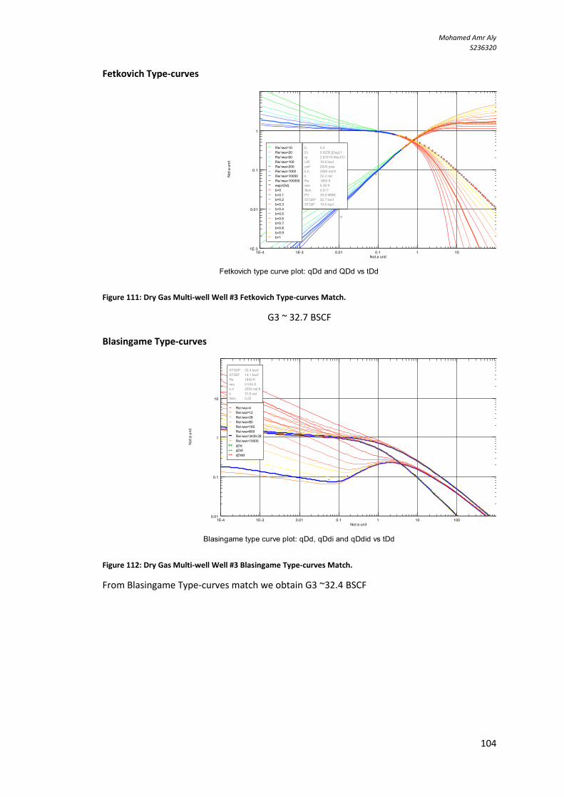
Mohamed Amr Aly

S236320

114



G3 ~ 32.7 BSCF




1E-4 1E-3 0.01 0.1 1 10Not a unit

1E-3

0.01

0.1

1

Not

a u

nit

Re/ rwa=10

Re/ rwa=20

Re/ rwa=50

Re/ rwa=100

Re/ rwa=200

Re/ rwa=1000

Re/ rwa=10000

Re/ rwa=100000

exp(-tDd)

b=0

b=0.1

b=0.2

b=0.3

b=0.4

b=0.5

b=0.6

b=0.7

b=0.8

b=0.9

b=1

b 0.4

Di 0.0235 [Day]-1

qi 2.81E+5 Mscf/ D

UR 19.9 bscf

pwf 2000 psia

k.h 2580 md.ft

k 32.2 md

Re 1850 ft

rwa 0.36 ft

Skin 0.617

PV 30.6 MMB

STGIIP 32.7 bscf

STGIP 14.5 bscf


1E-4 1E-3 0.01 0.1 1 10 100Not a unit

0.01

0.1

1

10

Not

a u

nit

Re/ rwa=4

Re/ rwa=12

Re/ rwa=28

Re/ rwa=80

Re/ rwa=160

Re/ rwa=800

Re/ rwa=3439.28

Re/ rwa=10000

qDd

qDdi

qDdid

STGIIP 32.4 bscf

STGIP 14.1 bscf

Re 1840 ft

rwa 0.535 ft

k.h 2550 md.ft

k 31.9 md

Skin 0.22


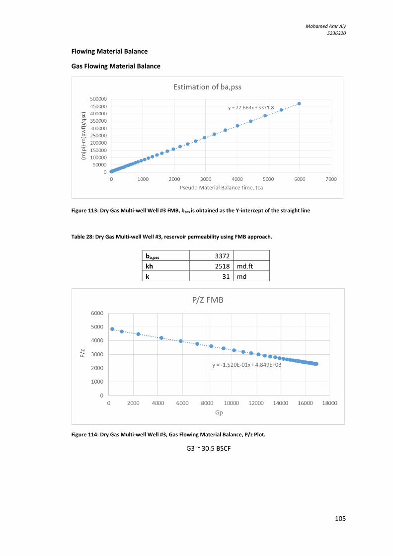
Mohamed Amr Aly

S236320

115






G3 ~ 30.5 BSCF

ba,pss 3372

kh 2518 md.ft

k 31 md

Mohamed Amr Aly

S236320

116

Agarwal Gardener


G3 ~ 32.6 BSCF



G2 ~ 34.9 BSCF

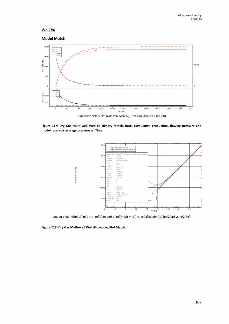
Mohamed Amr Aly

S236320

117

Well #4

Model Match

Figure 117: Dry Gas Multi-well Well #4 History Match. Rate, Cumulative production, flowing pressure and



0

1E+5

2E+5

3E+5

4E+5

Gas

rate

[Msc

f/D]

0

1E+10

Gas

vol

ume

[scf

]

q

Q

q model

Q model

0 2000 4000 6000 8000 10000 12000 14000 16000 18000 20000 22000 24000

Time [hr]

2500

3500

Pres

sure

[psi

a] Pi

p

Pbar


0.01 0.1 1 10 100 1000 10000 1E+5 1E+6Time [hr]

1000

10000

1E+5

1E+6

1E+7

1E+8

Gas

pot

entia

l [ps

i2/c

p]




Well Vertical



Tmin 0 hr

Tmax 23040 hr

Total Skin 0


k, average 30 md

Pi 4500 psia

STGIIP 131 bscf

STGIP 113 bscf

Qg(tmax) 18.3 bscf

Skin 0

Skin 0

Skin 0

Skin 0

Pi 4500 psia

k.h 2400 md.ft

k 30 md

TMatch 28300 [hr]-1



Ab. time (ta) N/ A

Q(ta) N/ A


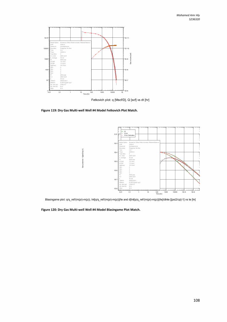
Mohamed Amr Aly

S236320

118



0.01 0.1 1 10 100 1000 10000 1E+5Time [hr]

1

10

100

1000

10000

1E+5

Gas

rate

[Msc

f/D]

1E+6

1E+7

1E+8

1E+9

1E+10

1E+11

Gas

vol

ume

[scf

]


Well Vertical



Tmin 0 hr

Tmax 23040 hr

Total Skin 0


k, average 30 md

Pi 4500 psia

STGIIP 131 bscf

STGIP 113 bscf

Qg(tmax) 18.3 bscf

Skin 0

Skin 0

Skin 0

Skin 0

Pi 4500 psia

k.h 2400 md.ft

k 30 md

TMatch 28300 [hr]-1



Ab. time (ta) N/ A

Q(ta) N/ A


0.01 0.1 1 10 100 1000 10000 1E+5 1E+6Time [hr]

1E-8

1E-7

1E-6

1E-5

1E-4

1E-3

0.01

Gas

pot

entia

l -1

[[psi

2/cp

]-1]

PI

PI Int.

PI Int. Derivative


Well Vertical



Tmin 0 hr

Tmax 23040 hr

Total Skin 0


k, average 30 md

Pi 4500 psia

STGIIP 131 bscf

STGIP 113 bscf

Qg(tmax) 18.3 bscf

Skin 0

Skin 0

Skin 0

Skin 0

Pi 4500 psia

k.h 2400 md.ft

k 30 md

TMatch 28300 [hr]-1



Ab. time (ta) N/ A

Q(ta) N/ A


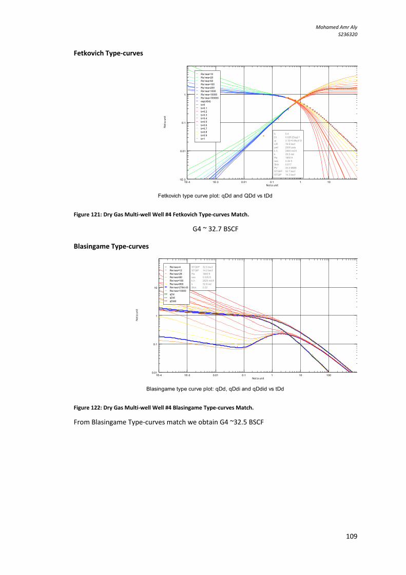
Mohamed Amr Aly

S236320

119



G4 ~ 32.7 BSCF




1E-4 1E-3 0.01 0.1 1 10Not a unit

1E-3

0.01

0.1

1

Not

a u

nit

Re/ rwa=10

Re/ rwa=20

Re/ rwa=50

Re/ rwa=100

Re/ rwa=200

Re/ rwa=1000

Re/ rwa=10000

Re/ rwa=100000

exp(-tDd)

b=0

b=0.1

b=0.2

b=0.3

b=0.4

b=0.5

b=0.6

b=0.7

b=0.8

b=0.9

b=1

b 0.4

Di 0.026 [Day]-1

qi 3.1E+5 Mscf/ D

UR 19.9 bscf

pwf 2000 psia

k.h 2840 md.ft

k 35.5 md

Re 1850 ft

rwa 0.36 ft

Skin 0.617

PV 30.6 MMB

STGIIP 32.7 bscf

STGIP 14.3 bscf


1E-4 1E-3 0.01 0.1 1 10 100Not a unit

0.01

0.1

1

10

Not

a u

nit

Re/ rwa=4

Re/ rwa=12

Re/ rwa=28

Re/ rwa=80

Re/ rwa=160

Re/ rwa=800

Re/ rwa=2764.43

Re/ rwa=10000

qDd

qDdi

qDdid

STGIIP 32.5 bscf

STGIP 14.2 bscf

Re 1840 ft

rwa 0.535 ft

k.h 2620 md.ft

k 32.8 md

Skin 0.22


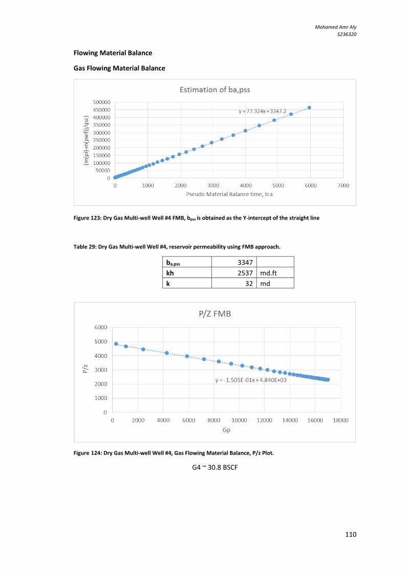
Mohamed Amr Aly

S236320

111





ba,pss 3347

kh 2537 md.ft

k 32 md


G4 ~ 30.8 BSCF

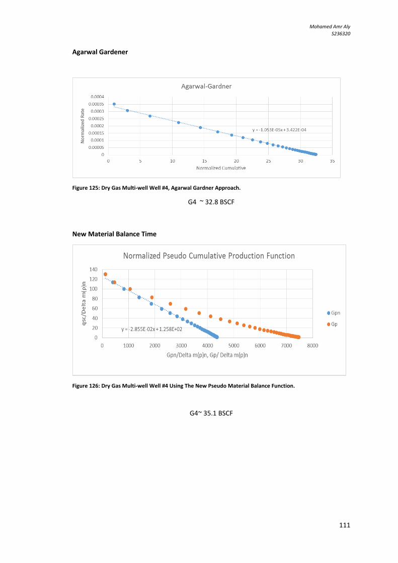
Mohamed Amr Aly

S236320

111

Agarwal Gardener


G4 ~ 32.8 BSCF



G4~ 35.1 BSCF

Rate Transient Analysis and Flowing Material Balance for ... · Rate Transient Analysis and Flowing...

Documents

Transcript of Rate Transient Analysis and Flowing Material Balance for ... · Rate Transient Analysis and Flowing...