OFDM SYSTEMS IN VEHICULAR ENVIRONMENT · stesso dovuta all’efietto Doppler. Negli algoritmi di...
156
UNIVERSIT ` A DEGLI STUDI DI PADOVA FACOLT ` A DI INGEGNERIA CORSO DI LAUREA IN INGEGNERIA DELLE TELECOMUNICAZIONI TESI DI LAUREA SPECIALISTICA DATA DECODING AIDED CHANNEL ESTIMATION TECHNIQUES FOR OFDM SYSTEMS IN VEHICULAR ENVIRONMENT Relatore: Ch.mo Prof. Silvano Pupolin Correlatori: Massimiliano Siti, Antonio Assalini Laureando: Andrea Agnoletto Padova, 8 Marzo 2010
Transcript of OFDM SYSTEMS IN VEHICULAR ENVIRONMENT · stesso dovuta all’efietto Doppler. Negli algoritmi di...

UNIVERSITA DEGLI STUDI DI PADOVA
FACOLTA DI INGEGNERIA
CORSO DI LAUREA IN INGEGNERIA DELLE TELECOMUNICAZIONI
TESI DI LAUREA SPECIALISTICA
DATA DECODING AIDED
CHANNEL ESTIMATION TECHNIQUES FOR
OFDM SYSTEMS IN VEHICULAR ENVIRONMENT
Relatore: Ch.mo Prof. Silvano Pupolin
Correlatori: Massimiliano Siti, Antonio Assalini
Laureando: Andrea Agnoletto
Padova, 8 Marzo 2010

e-mail: [email protected]

Prefazione
L’oggetto del presente lavoro di tesi e costituito dallo studio e sviluppo di algoritmi di
inseguimento di canale per sistemi basati su una modulazione di tipo Orthogonal Fre-
quency Division Multiplexing (OFDM), con riferimento allo standard IEEE802.11p
per comunicazioni mobili di tipo Wireless Local Area Network (WLAN), tra veicolo e
veicolo e tra veicolo e infrastruttura. La caratteristica principale dei sistemi wireless
in ambiente veicolare e la presenza dell’effetto Doppler dovuto alla velocita relativa
tra trasmettitore e ricevitore che rende il canale wireless tempo variante.
I primi capitoli della presente tesi sono dedicati all’analisi delle caratteristiche e
della modellizzazione del canale wireless in ambiente veicolare, del sistema OFDM,
dello standard IEEE 802.11p proposto per comunicazioni wireless in ambiente ve-
icolare. I capitoli conclusivi invece presentano rispettivamente il lavoro compiuto
riguardo alcune differenti opzioni di algoritmi di stima di canale per sistemi OFDM,
e l’analisi e implementazione di tecniche di stima dell’effetto Doppler presente negli
ambienti veicolari.
I due principali schemi di stima e inseguimento di canale investigati sono basati
sull’utilizzo del decodificatore di Viterbi per ricostruire il simbolo OFDM ricevuto e
utilizzarlo nella stima di canale. Il primo schema, di tipo iterativo, e piu complesso
dal punto di vista computazionale e implementativo rispetto a schemi di stima e
inseguimento di canale che non utilizzano il decodificatore: per ogni simbolo OFDM
ricevuto sono effettuate due iterazioni del decodificatore di Viterbi (che e il blocco
computazionalmente piu oneroso): in tale schema, i dati in uscita dalla prima iter-
azione di decodifica di Viterbi sono utilizzati per ricostruire la sequenza di simboli
complessi trasmessa, i quali a loro volta servono per ripetere la stima di canale da
utilizzare per una successiva e finale equalizzazione e decodifica (seconda passata di
Viterbi) del simbolo OFDM in oggetto.
Il secondo schema proposto e di tipo non iterativo, ovvero prevede una sola iter-
azione del decodificatore di Viterbi. per decodificare i bit di informazione corrispon-
denti al simbolo OFDM ricevuto all’istante sotto osservazione, e al tempo stesso per
ricostruire la sequenza di simboli complessi trasmessi da utilizzare per raffinare la
stima di canale, che sara’ utilizzata per l’equalizzazione del simbolo OFDM succes-
sivo. Ne risulta uno schema con impatto di complessita computazionale confrontabile
con gli schemi che non utilizzano il decodificatore di Viterbi nella stima di canale.
Le simulazioni di prestazione ottenute con i due schemi mostrano che lo schema
iii

non iterativo produce risultati confrontabili con gli stessi ottenuti nel caso iterativo,
peggioramenti maggiori di 1 dB di rapporto segnale-rumore si osservano solo negli
scenari simulati con velocita relative tra trasmettitore e ricevitore molto elevate. Dai
risultati ottenuti si osserva in particolare che entrambi gli schemi inseguono molto
bene il canale e significative perdite in termini di rapporto segnale-rumore rispetto al
caso di conoscenza ideale del canale si notano solo in un ristretto numero di scenari
simulati, caratterizzati da alti bitrate e alte velocita relative.
A completamento del capitolo in oggetto sono state descritte ulteriori analisi sugli
errori residui in uscita dal decodificatore di Viterbi. In entrambi gli algoritmi men-
zionati, la equalizzazione di partenza del simbolo OFDM in oggetto e effettuata a
partire dalla stima di canale derivata all’istante di tempo precedente, e percio gen-
eralmente affetta da degradazione dovuta all’effetto Doppler. Questa considerazione
ha motivato l’ultimo argomento del capitolo in esame, ovvero la analisi e simulazione
di metodi di predizione della stima di canale per compensare la degradazione dello
stesso dovuta all’effetto Doppler.
Negli algoritmi di inseguimento di canale citati sopra, la stima di canale viene
ripetuta per ogni simbolo OFDM ricevuto. Con l’obiettivo di ridurre il consumo
di energia, e stato analizzata la possibilita di ridurre la frequenza di aggiornamento
della stima di canale senza degradare significativamente le prestazioni. L’ultimo
capitolo e pertanto dedicato alla presentazione di metodi per la derivazione di un
valore di frequenza di aggiornamento in funzione della velocita relativa, per una
massima degradazione tollerabile delle prestazioni, imposta a priori. Prerequisito
per l’applicabilita’ di tale idea e la conoscenza al ricevitore della velocita relativa tra
trasmettitore e ricevitore. Allo scopo, due differenti algoritmi di stima della velocita
in banda base sono stati modellati con applicazione ai sistemi veicolari, e confrontati.
Previa l’introduzione di una opportuna modifica rispetto a quanto presentato in let-
teratura, simulazioni di stima della velocita’ relativa hanno mostrato che uno dei due
metodi analizzati e’ potenzialmente adeguato allo scopo. A conclusione del capitolo
sono riportate le curve di prestazione in termini di tasso di errore di pacchetto WLAN
verso rapporto segnale-rumore, in cui la frequenza di aggiornamento della stima di
canale e determinata a partire dalla stima di velocita ottenuta utilizzando lo stima-
tore di velocita ritenuto piu idoneo all’utilizzo in ambiente veicolare.
Contents
Introduction vii
1 The Wireless Channel 1
1.1 Introduction . . . . . . . . . . . . . . . . . . . . . . . . . . . . . . . . 1
1.1.1 Path loss . . . . . . . . . . . . . . . . . . . . . . . . . . . . . . 2
1.1.2 Shadowing effect . . . . . . . . . . . . . . . . . . . . . . . . . 3
1.1.3 Doppler spread . . . . . . . . . . . . . . . . . . . . . . . . . . 5
1.1.4 Statistical multipath channels . . . . . . . . . . . . . . . . . . 7
1.2 Wireless channel models . . . . . . . . . . . . . . . . . . . . . . . . . 9
1.2.1 Tapped-delay-line channel model . . . . . . . . . . . . . . . . 9
1.2.2 Wireless channel models for Vehicular Environment . . . . . . 11
2 Orthogonal Frequency Division Multiplexing 17
2.1 OFDM systems . . . . . . . . . . . . . . . . . . . . . . . . . . . . . . 17
2.1.1 System model . . . . . . . . . . . . . . . . . . . . . . . . . . . 18
2.2 OFDM System with cyclic prefix . . . . . . . . . . . . . . . . . . . . 20
2.2.1 Equalization in OFDM systems . . . . . . . . . . . . . . . . . 24
3 IEEE 802.11p Standard for WLAN in Vehicular Environment 29
3.1 Introduction . . . . . . . . . . . . . . . . . . . . . . . . . . . . . . . . 29
3.2 IEEE 802.11p Physical layer . . . . . . . . . . . . . . . . . . . . . . . 30
3.2.1 General description . . . . . . . . . . . . . . . . . . . . . . . . 30
3.2.2 OFDM parameters . . . . . . . . . . . . . . . . . . . . . . . . 32
3.2.3 Frame structure . . . . . . . . . . . . . . . . . . . . . . . . . . 33
3.2.4 Scrambling, coding, interleaving and mapping . . . . . . . . . 39
3.2.5 Implemented MATLAB model of IEEE 802.11p . . . . . . . . 45
v

vi Contents
4 Channel estimation algorithms for OFDM systems 47
4.1 Channel estimation algorithms . . . . . . . . . . . . . . . . . . . . . . 47
4.1.1 Least Square channel estimation . . . . . . . . . . . . . . . . . 48
4.1.2 TD-LS reduced rank channel estimation . . . . . . . . . . . . 49
4.1.3 Modified reduced rank LS channel estimation . . . . . . . . . 51
4.1.4 MMSE channel estimation . . . . . . . . . . . . . . . . . . . . 52
4.2 Channel length estimation . . . . . . . . . . . . . . . . . . . . . . . . 55
5 Decision directed channel estimation for mobile OFDM systems 57
5.1 Introduction . . . . . . . . . . . . . . . . . . . . . . . . . . . . . . . . 57
5.1.1 Vehicular channel time invariance assessments . . . . . . . . . 58
5.1.2 Channel tracking algorithms . . . . . . . . . . . . . . . . . . . 59
5.2 Decision directed channel estimation . . . . . . . . . . . . . . . . . . 60
5.3 Data decoding aided channel estimation . . . . . . . . . . . . . . . . 63
5.3.1 First scheme: iterative data decoding aided CE . . . . . . . . 63
5.3.2 Second scheme: non-iterative data decoding aided CE . . . . . 65
5.3.3 Performance results . . . . . . . . . . . . . . . . . . . . . . . . 67
5.4 Linear prediction . . . . . . . . . . . . . . . . . . . . . . . . . . . . . 90
5.4.1 Linear MMSE prediction . . . . . . . . . . . . . . . . . . . . . 90
5.4.2 AR(N) model . . . . . . . . . . . . . . . . . . . . . . . . . . . 97
5.4.3 Kalman filter . . . . . . . . . . . . . . . . . . . . . . . . . . . 100
6 Doppler estimation techniques for OFDM-based vehicular systems107
6.1 Problem definition: impact of CE occurrence on PHY performance . 108
6.2 Techniques for Doppler spread estimation . . . . . . . . . . . . . . . . 114
6.2.1 Hybrid autocorrelation-based Doppler spread estimator . . . . 114
6.2.2 Doppler spread estimation based on ZCR measurement . . . . 127
6.3 Performance curves with variable CE occurrence . . . . . . . . . . . . 131
7 Conclusions 139
Bibliography 141

Introduction
During the last two decades wireless communications have become one of the key
sectors in worldwide economy and everyday life. Examples of this arise from wireless
local area networks (WLANs) to mobile phones, Bluetooth personal devices and
satellite television broadcasting; all these technologies have become fundamental and
new fields of application for wireless communications are continuously emerging.
Providing wireless communications in high mobility scenarios is the new challenge
derived from the necessity to guarantee wireless access in the most practical real
situations.
In this contest Wireless Access in Vehicular Environment (WAVE) is a technology
that provides connectivity in the Dedicated Short Range Communications (DSRC)
frequencies for applications suitable in the area of the Intelligent Transport System
(ITS). An official classification of ITS applications does not exist. However, poten-
tially a vast set of applications can be provided, ranging from driver safety increase,
which is the main purpose of these networks, to traffic flow monitoring and congestion
mitigation, or electronic tolling collection. The grant of WAVE is to provide wireless
low latency, geographically local, high data rate, and high mobility communications
whose typical applications are in the area of ITS.
This kind of applications are considered critical for the next future: during the last
years safety in vehicular context has been greatly improved with new technologies
including various kind of sensors that continuously monitor the road to prevent
accidents. The continuous increase of the number of vehicles, and consequently of
collisions, underlines the importance of inter-vehicle communications, considered a
key-factor in future preventing accidents and increasing safety.
A contextualization to the vehicular environment in the sense of wireless com-
munications is given by wireless local area networks (WLANs). Typical scenarios in
which WAVE is supposed to focus are small aggregates of vehicles. In this context
the IEEE 802.11 set of Standards for WLANs has been extended with IEEE 802.11p
vii

viii Introduction
that is a proposed enhancement to IEEE 802.11 in order to guarantee reliable data
exchange between high-speed vehicles and between vehicles and the roadside infras-
tructure in the licensed ITS band of 5.9 GHz (5.85-5.925 GHz). Based on the Or-
thogonal Frequency Division Multiplexing (OFDM) system, IEEE 802.11p provides
physical and Medium Access Control (MAC) layers specifications.
Aim of this thesis is the study of the issues related to the wireless channel es-
timation in a time-varying frequency-selective contest for OFDM systems. Starting
from the pre-existent work, the focus will be on the decision-directed channel estima-
tion (DD-CE) techniques. After a review on the existent work, DD-CE algorithms
with forward error correction (FEC) will be investigated by a comparison in terms of
performance and complexity. DD-CE with FEC shows great improvements in perfor-
mance even in high-mobility scenarios with respect to the DD-CE schemes without
FEC, but at the cost of higher system complexity.
Despite that, two further improvements to the investigated channel tracking al-
gorithms have been evaluated. The first, is motivated by the performance gap still
observable compared to the ideal case for very challenging scenarios like high rela-
tive speed (≥ 120 Km/h), long WLAN packets (≥ 400 byte), high modulation orders
(64-QAM). Linear prediction of the channel estimate is considered in order to com-
pensate the degradation of the channel estimation due to the Doppler effect with
comparisons between optimal and sub-optimal well-known algorithms.
As a second improvement to the data decoding-aided DD-CE scheme, the selec-
tion of the CE occurrence as a function of the estimated relative speed between trans-
mitter and receiver is discussed. This may be useful in practical portable systems to
reduce processing time and/or power consumption. In particular it will be presented
a strategy to select the CE occurrence based on the relative speed between transmit-
ter and receiver and a maximum (set a-priori by the designer) tolerable degradation
of the SNR seen at the receiver, due to the Doppler effect.
The relative speed between transmitter and receiver is a function of the Doppler
spread; this motivates the assessment of the state-of-the-art Doppler spread estima-
tion algorithms and their application to vehicular systems. The most effective in
vehicular environment will be then taken into account. Finally, the performance re-
sults obtained with decreased CE occurrence based on the estimated relative speed,
obtained with the selected Doppler spread estimator, will be presented.
This thesis is organized as follows.

Introduction ix
Chapter 1. This chapter deals with the description of the time-varying frequency
selective wireless channel. The concepts of path loss, shadowing effect, Doppler shift
and multipath fading are investigated. The modeling of the discrete-time wireless
channel is presented. Finally, wireless channel models suitable for vehicular environ-
ment are presented.
Chapter 2. In this chapter Orthogonal Frequency Division Multiplexing (ODFM)
system is analyzed: the general OFDM system and a simplified model employing
prototype filters are presented. The filterless OFDM system with cyclic prefix is
described: under the assumption of absence of noise, it guarantees the reconstruction
of the transmitted symbol with a simple zero-forcing equalization even for frequency-
selective channels.
Chapter 3. This chapter describes the Wireless Access in Vehicular Environment
technology as the system considered to provide wireless connectivity in vehicular
environment. In this chapter the description of the IEEE 802.11p physical layer is
also included together with the generation procedure of the physical layer data unit.
Chapter 4. Chaper 4 deals with channel estimation (CE) techniques. First a
brief general subdivision of the various CE techniques is given. Then various CE
techniques suitable for IEEE 802.11p are presented together with the evaluation of
the relative CE error. The eviewed approaches are reported in increasing order of
complexity.
Chapter 5. This chapter deals with DD-CE techniques with particular focus on
the DD-CE algorithms with forward error-correction (FEC) due to the decoder. The
improvements in performance with respect to the case with no FEC are shown. Two
FEC aided DD-CE algorithms are proposed and compared in terms of complexity
and performance. Moreover linear prediction of the channel is studied; a comparison
in terms of performance and complexity between the optimal and a sub-optimal
approach is also included.
Chapter 6. In this chapter the problem of evaluating the impact of CE occurrence
on link performance is presented. It is shown that the time variation of the channel
due to the relative speed between transmitter and receiver is related to the Doppler
x Chapter 0. Introduction
spread, and consequently to the relative speed between transmitter and receiver. A
strategy to decrease the CE occurrence as a function of the relative speed between
transmitter and receiver is presented, in order to reduce processing time and power
consumption. Consequently two different Doppler spread estimation algorithms are
studied and reviewed. The most effective in vehicular environment will be then taken
into account. Finally simulation results with decreased CE occurrence, selected as
a function of the estimated relative speed and a maximum tolerable degradation of
the signal-to-noise ratio seen at the receiver, are presented.
Chapter 7. Chapter 7 reports a brief conclusion of this thesis.
Chapter 1
The Wireless Channel
1.1 Introduction
In wireless communications the wireless radio channel is the source of the various
degradations such as attenuation, noise and interferences that afflict the signal at
the receiver with respect to the transmitted signal. These elements have a nature
intrinsically difficult to predict. Moreover in vehicular environment all these degra-
dations of the signal are not static: the time-varying nature of the scenario causes
a continuous variation of the wireless channel characteristics. To better understand
and model the time-varying wireless channel the different aspects of attenuation,
noise contribution, interference and time-varying effects will be analyzed.
The additive white Gaussian noise (AWGN) is the main source of noise in a
wireless system and is the model for the thermal noise generated at the receiver.
The various degradations that afflict the received signal are typical grouped in two
main categories:
• large-scale fading takes into account the attenuation caused by the distance
between the transmitter and the receiver that is usually defined path loss and
the slow fluctuation of the receiver power due to large obstacles (with respect
to the wavelength) between the receiver and the transmitter as buildings and
hills, typically referred to as shadowing ; these degradations of the received
signal are usually frequency independent;
• small-scale fading takes into account the reflection and scattering introduced
by small obstacles (with a spatial scale of the order of the wavelength) as
1

2 Chapter 1. The Wireless Channel
vehicles or small objects; these kind of interferences are typically frequency
selective.
The time-varying nature of the wireless channel is given by the movement of
either the transmitter or the receiver or of the reflectors in the transmission paths.
The consequence is a change in the amplitude, distortion and time of arrival of the
different rays seen at the receiver. This effect is known as Doppler shift.
In vehicular environment these non-static elements do not generally afflict the
large-scale fading: the comprehensive geometry of large obstacles is almost static in
the transmission time considered for the typically achievable relative speeds. On the
contrary small-scale fading has a time-varying nature: the variations of the scattering
and reflections generated by small obstacles is not negligible in vehicular scenarios.
Under these assumptions the wireless channel has a time-varying frequency-
selective nature. In the following these aspects introduced will be investigated in
order to model the wireless channel in vehicular environment.
1.1.1 Path loss
The simplest scenario for wireless communication is the free space: a transmitter
and a receiver at distance d from each other with no obstacles. In this assumption
the signal propagates along a straight line and no distortion occurs. The channel
model associated with this transmission is called a line-of-sight (LOS) channel, and
the corresponding received signal is called the LOS signal or ray. Free space path
loss attenuates the transmitted signal by the factor:
Pr
Pt
= G1G2
(λ
4πd
)2
(1.1)
where Pt [W] and Pr [W] are, respectively, the power of the transmitted and received
signals, G1 and G2 are the gains of the transmitting and receiving antennas and λ
[m] is the wavelength of the radio wave. Therefore, the received signal power falls
off inversely proportional to the square of the distance d [m] between the transmit
and receive antennas.
Equation (1.1) holds for non-LOS components too tacking into account that
d represents the total distance covered by the ray. The received signal power is
also proportional to the square of the signal wavelength, so as the carrier frequency
increases, the received power decreases.

1.1. Introduction 3
Environment γ range
Urban macro cells 3.7− 6.5
Urban micro cells 2.7− 3.5
Office Building (same floor) 1.6− 3.5
Office Building (multiple floors) 2− 6
Store 1.8− 2.2
Factory 1.6− 3.3
Home 3
Table 1.1: Typical Path Loss Exponents
In cases of multipath propagation ray tracing can be useful to study the attenu-
ation of the received power due to the combined path-loss; for example the two ray
tracing model sums the effect of the LOS component with the one reflected by the
ground.
A number of path loss models have been developed to describe free-space atten-
uation in typical wireless environments such as large urban macro cells and urban
micro cells. These models are mainly based on empirical measurements over a given
distance in a given frequency range and a particular geographical area or building.
The complexity of signal propagation in wireless mobile environments makes very
difficult to obtain a general model that characterizes path loss accurately across
different environments. However, for general trade-off analysis of various system
designs it is sometimes convenient to use a simpler model such as the following:
a(d) =Pr
Pt
= Ka
(d0
d
)γ
(1.2)
where Ka is a constant that depends on the antenna characteristics and on the
average channel attenuation, d0 [m] is a reference distance for the antenna far-field
region, and γ depends on the type of environment. In table 1.1.1 are reported some
examples of measured values of γ for different scenarios [2].
1.1.2 Shadowing effect
Big obstacles between the transmitter and the receiver as buildings or hills cause a
random attenuation of the signal with respect to the average received power. This
effect is commonly referred to as shadowing. When the attenuation is very strong,

4 Chapter 1. The Wireless Channel
the signal can be severely attenuated.
In order to model the shadowing effect the ratio of transmit-to-receive power is
defined as ψ(t) = Pt(t)/Pr(t). With this notation the power attenuation due to the
shadowing effect at time t is Pr(t)/Pt(t) = 1/ψ(t).
From empirical studies it turned out that the shadowing is distributed accord-
ing to a log-normal distribution, and this is the most common model for this phe-
nomenon. The distribution of these fluctuations of the power attenuation ψ is given
by [2]:
p(ψ) =10/ ln 10
ψ√
2πσ2ψdB
exp
−(10 log10 ψ − µψdB
)2
2σψ2dB
ψ > 0 (1.3)
where µψdBis the expectation of ψdB = 10 log10(ψ) in dB and σ2
ψdBis the standard
deviation of ψ, also in dB. The expectation can be based on an analytical model or
empirical measurements. The expectation of ψ(t) can be obtained from 1.3 as:
µψ = E [ψ(t)] = exp
[µψdB
10/ ln 10+
σ2ψdB
2(10/ ln 10)2
](1.4)
and the conversion from the linear mean (in dB) to the log mean is:
10 log10 µψ = µψdB+
σ2ψdB
20/ ln 10. (1.5)
After a change of variables it results that the distribution of the dB value of ψ(t) is
Gaussian with mean µψdBand standard deviation σ2
ψdB,
p(ψdB) =1√
2πσ2ψdB
exp
−(ψdB − µψdB
)2
2σ2ψdB
(1.6)
The combined effect of path loss and shadowing plays a fundamental role in
wireless systems design. In fact, usually, there is a minimum received power level
Pmin, below which the performance becomes unacceptable. The outage probabil-
ity poutage(Pmin, d) under path loss and shadowing is defined as the probability
that the received power at a given distance d, Pr(d, t) is lower than Pmin, that is
poutage(Pmin, d, t) = P [Pr(d, t) < Pmin]. Pmin also depends on the sensitivity of the
receiver. Combining path loss and shadowing model, the outage probability be-
comes [2]

1.1. Introduction 5
Figure 1.1: Illustration of the Doppler spread
poutage = P [Pr(d, t) < Pmin] =
1−Q
(Pmin − (Pt(t)− 10 log10 Ka − 10γ log10(d/d0))
σψdB
)(1.7)
where
Q(z) = p(x > z) =
+∞∫
z
1
2πe−y2/2dy (1.8)
is the complementary Gaussian distribution function.
1.1.3 Doppler spread
Doppler spread, or Doppler shift, is the frequency shift that the receiver undergoes
with respect to the transmitted frequency. This is caused by the relative motion
between transmitter and receiver.
With reference to Figure 1.1 let TX be the transmitter and RX the receiver that
moves from a point P to a point Q with speed v. The variation of distance between
the two equipments is ∆l = v∆t cos θ where ∆t is the time the receiver takes to go
from P to Q, θ is the angle of incidence of the signal with respect to the direction
of motion and v cos θ is the relative speed between the transmitter and the receiver.
The phase variation due to this difference in the path length is
∆φ =2π∆l
λ=
2πv∆t cos θ
λ(1.9)
where λ is the wavelength of the transmitted signal. The Doppler frequency is then
given by the relation
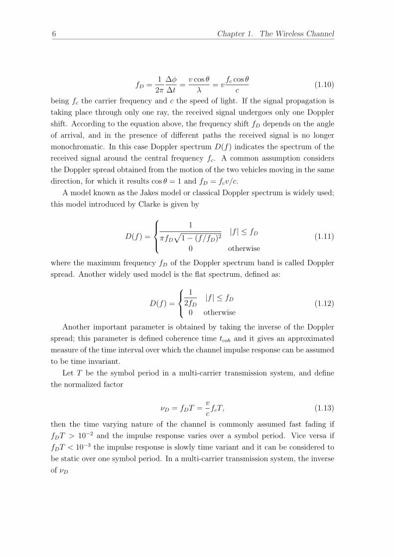
6 Chapter 1. The Wireless Channel
fD =1
2π
∆φ
∆t=
v cos θ
λ= v
fc cos θ
c(1.10)
being fc the carrier frequency and c the speed of light. If the signal propagation is
taking place through only one ray, the received signal undergoes only one Doppler
shift. According to the equation above, the frequency shift fD depends on the angle
of arrival, and in the presence of different paths the received signal is no longer
monochromatic. In this case Doppler spectrum D(f) indicates the spectrum of the
received signal around the central frequency fc. A common assumption considers
the Doppler spread obtained from the motion of the two vehicles moving in the same
direction, for which it results cos θ = 1 and fD = fcv/c.
A model known as the Jakes model or classical Doppler spectrum is widely used;
this model introduced by Clarke is given by
D(f) =
1
πfD
√1− (f/fD)2
|f | ≤ fD
0 otherwise
(1.11)
where the maximum frequency fD of the Doppler spectrum band is called Doppler
spread. Another widely used model is the flat spectrum, defined as:
D(f) =
1
2fD
|f | ≤ fD
0 otherwise(1.12)
Another important parameter is obtained by taking the inverse of the Doppler
spread; this parameter is defined coherence time tcoh and it gives an approximated
measure of the time interval over which the channel impulse response can be assumed
to be time invariant.
Let T be the symbol period in a multi-carrier transmission system, and define
the normalized factor
νD = fDT =v
cfcT, (1.13)
then the time varying nature of the channel is commonly assumed fast fading if
fDT > 10−2 and the impulse response varies over a symbol period. Vice versa if
fDT < 10−3 the impulse response is slowly time variant and it can be considered to
be static over one symbol period. In a multi-carrier transmission system, the inverse
of νD

1.1. Introduction 7
NS =1
νD
=1
fDT(1.14)
gives an approximated number of consecutive symbols where the channel can be
considered time invariant.
1.1.4 Statistical multipath channels
When a pulse is transmitted over a time-dispersive channel the received signal will
be viewed as a train of pulses, where a pulse corresponds to either the LOS compo-
nent, or a distinct path associated with a scatterer or cluster of scatterers. A very
important characteristic of a multipath environment is the time delay spread. The
delay spread equals the time interval between the arrival of the first and last ray [1].
The baseband expression of a multipath channel impulse response seen at time t
in response to an impulse applied at time t − τ with Lch paths seen at the receiver
is:
h(t, τ) =
Lch−1∑
l=0
hl(t)δ(τ − τl(t)) (1.15)
where δ(·) is the Dirac pulse, hl(t) is the complex valued gain of the l−th path seen
at the receiver with delay τl(t) and t ∈ R is the observation time.
The presented path loss and shadowing models can be grouped together and then
the wireless channel model becomes:
h(t, τ) =√
(1/ψ(t))√
a(d)
Lch−1∑
l=0
hl(t)δ(τ − τl(t)) (1.16)
where a(d) is the path loss attenuation (1.2) and d is the distance between transmitter
and receiver in meters at time t. Through the model (1.16) the transmission link
is modeled as a linear filter with a time-varying impulse response; the non-static
behavior of the channel is caused by changes in the environment as the relative
motion between transmitter and receiver.
In case time variations can be neglected for the system of interest, i.e. hl(t) ' hl
and τl(t) ' τl, the model is referred to as slow fading. On the other hand, the Doppler
effect introduced in subsection 1.1.3 must be taken into account for vehicular systems,
as shown in 3.1.

8 Chapter 1. The Wireless Channel
In a digital transmission system the effect of multipath depends on the duration
of the symbol period compared to the length of the channel impulse response. If the
duration of the channel impulse response is very low compared to the duration of
the symbol period, then a model with only one path is adeguate and results in a flat
fading channel. In more general conditions, a suitable model has to include several
paths. A typical statistical description of the gains hl(t) is given by [1]:
hl(t) =
C + h0(t) l = 0
hl(t) l = 1, . . . , Lch − 1(1.17)
where C is a real-valued constant which takes into account the LOS component
and hl(t) are complex-valued Gaussian random variables with zero mean. The phase
of hl(t) is uniformly distributed in [0, 2π). Therefore the first path contains a deter-
ministic component added to a random one. The other paths are assumed to be ran-
dom. The distribution of |h0| results a Rice distribution while |hi|, i = 1, . . . , Lch−1
have Rayleigh distribution. In particular defining
hl(t) =hl(t)√
E[|hl(t)|2](1.18)
it turns that
p|h0|(ψ) = 2(1 + K)ψ exp[−K − (1 + K)ψ2]I0
(2ψ
√K(1 + K)
)1(ψ)
p|hl|(ψ) = 2ψe−ψ2
1(ψ)(1.19)
where I0(·) is the modified Bessel function of the first type and zero-th order and
1(ψ) equal to 1 for ψ > 0 and to 0 for ψ < 0. In presence of the LOS component
the parameter K = C2/ E[|h0|2], known as Rice factor, is equal to the ratio between
the power of the LOS component and the power of the reflected component. For a
model with several paths, Lch > 1, K is defined as K = C2/Mc, where Mc is the
statistical power of all reflected and/or scattered components. Assuming that the
power delay profile (PDP) of the channel is normalized, that is
Lch−1∑i=0
E[|hi(t)|2] =
Lch−1∑i=0
σ2hi
= 1 (1.20)
it results that C =√
K/(K + 1). If the LOS component is absent, C = 0 and all
gains have a Rayleigh distribution. Typical values of K are 3 and 10 dB, if no LOS
exists then K = 0.
1.2. Wireless channel models 9
1.2 Wireless channel models
1.2.1 Tapped-delay-line channel model
In order to introduce a time-varying frequency-selective channel model in discrete
time it is firstly described a continuous time channel model that takes into account
all the aspects presented previously.
Assuming that signal propagation occurs through a large number of paths, it has
been shown that the baseband equivalent channel impulse response can be repre-
sented with good approximation as a time-varying complex-valued Gaussian random
process h(t, τ) where h(t, τ) is the output of the channel at instant t in response to
an ideal impulse applied at instant t− τ .
A widely used statistical model is the wide-sense stationary uncorrelated scat-
tering (WSS-US) channel model. The WSS property implies that the second-order
statistics of the channel are stationary; US model means that the paths that ar-
rive with different delays are uncorrelated. In this way the cross-correlation of the
channel evaluated for delays τ, τ −∆τ at time instants t and t−∆t is
rh(t, t−∆t; τ −∆τ) = E[h(t, τ)h∗(t−∆t, τ −∆τ)] = rh(∆t, τ)δ(∆τ). (1.21)
This means that the autocorrelation of the channel is zero for impulse responses
considered at different delays. Moreover, as h(t, τ) is stationary in t, the autocorrela-
tion depends only on the difference of the times at which the two impulse responses
are evaluated. Imposing ∆t = 0 the power delay profile can be defined as:
M(τ) = E[|h(τ)|2] (1.22)
and it represents the power behavior of the channel impulse response for a given
delay. In presence of multipath, another useful parameter is the root-mean square
time delay spread τrms, given by
τ 2rms =
∫(u− τ)2M(u)du∫
M(u)du=
∫u2M(u)du∫M(u)du
− τ 2 (1.23)
with
τ =
∫uM(u)du∫M(u)du
(1.24)
that expresses the channel dispersion in the time domain. It stands out that (1.23)
expresses the average root-mean square time delay spread τrms as the squared root of

10 Chapter 1. The Wireless Channel
the second-order central moment of the power delay profile. For a Rayleigh channel
model, typical curves for M(τ) can be Gaussian unilateral or Exponential unilateral.
The inverse of the root-mean square time delay spread τrms is proportional to the
coherence bandwidth of the channel; it is often approximated as Bcoh∼= 1/(5τrms)
that is a measure of the frequency selectivity of the channel. In particular, if Bcoh
is lower than the transmission rate of the system, then the channel is considered
frequency selective, otherwise it is said to be a flat fading channel.
For many purposes, it is useful to approximate the continuous time wireless link
by a discrete-time channel with sampling period Tc, often assumed equal to the chip
period of the multicarrier transmission, that is Tc = 1/B where B is the transmission
bandwidth of the multicarrier system.
The discrete time model is obtained by sampling M(τ) with sampling period
Tc and by truncating the channel impulse response so that it includes only a finite
number of propagation paths, where the less significant paths can be neglected. For a
fixed t, the time axis is divided into equal intervals of duration Tc. With reference to
(1.15) the paths are restricted to lie in one of the time interval bins. If Lch represents
the number of significant paths, then the multipath spread of this discrete model is
(Lch − 1)Tc.
Thus, in the discrete time domain the multipath wireless channel is modeled as
a time-varying discrete WSS-US channel having Tc spaced taps components as
h(kTc,mTc) =
Lch−1∑
l=0
hl(kTc)δ(mTc − lTc). (1.25)
and the autocorrelation function of h(kTc,mTc) for delays ∆t, ∆τ is
rh(kTc, kTc −∆t; mTc,mTc −∆τ) = rh(∆t; ∆τ) =
Lch−1∑
l=0
rhl(∆t)δ(∆τ − lTc) (1.26)
where rhl(∆t) is the autocorrelation function of the l−th tap evaluated for a delay
∆t. If the transmitter and the receiver are in a static position, that is v = 0, then all
the taps are constant during the transmission. In a mobile system, if a NLOS model
is considered, all the taps hl(kTc) are complex-valued Gaussian stationary processes
with zero mean. The Doppler spectrum results the Fourier transform of rhl(∆t):
D(f) =
+∞∫
−∞
rhl(∆t)e−j2πf∆tdf. (1.27)
1.2. Wireless channel models 11
A widely considered Doppler spectrum in outdoor scenario is the Jakes model
(1.11) that is applied independently to every tap.
The overall power is normalized to
Lch−1∑
l=0
E[|hl(kTc)|2] =
Lch−1∑
l=0
σ2hl
= 1 (1.28)
where σ2hl
is the variance of each tap.
Let the channel impulse response at time instant kTc be defined in the M × 1
vector form as h(kTc) = [h0(kTc), h1(kTc), . . . , hLch−1(kTc), 0, . . . , 0]T , where the first
Lch entries corresponds to the non-zero taps and the last M − Lch are set to zero.
Let FM be the M ×M discrete Fourier transform (DFT) matrix, with the (m,n)th
entry equals to [FM ]m,n = exp(−j2πmn/M). Then, the channel frequency response
(CFR), in vector form, is given by
H(kTc) = FMh(kTc) (1.29)
From equation (1.29), the M×1 vector H(kTc) must be interpreted as the CFR of
the channel observed at time kTc. For any m = 0, 1, . . . ,M−1 the m−th component
of H can be modeled with a complex Gaussian random variable with zero mean and
variance
σ2H =
Lch−1∑
l=0
σ2hl
= 1 (1.30)
and this implies that the channel frequency response samples Hm, m = 0, . . . , M−1,
are identically distributed, Gaussian, with zero mean and variance σ2H .
1.2.2 Wireless channel models for Vehicular Environment
In literature various channel models suitable for vehicular environment have been
proposed, some of them are based on extensive measurements taken in outdoor en-
vironment. In [5] six small-scale fading channel models for wireless communication
systems in vehicular environment are proposed from Georgia Tech university and are
characterized by LOS scenarios. These models have been cited in IEEE 802.11p as
informative examples but not as official reference models for the standard.
Nevertheless, in vehicular environment there may be conditions in which a LOS
component is not present, which are also the most critical for the physical layer

12 Chapter 1. The Wireless Channel
performance. Therefore, it is important to take into account also non-LOS (NLOS)
scenarios when evaluating the communication system performance.
For this reason in the following evaluations indoor NLOS scenarios proposed by
ETSI have been taken into account.
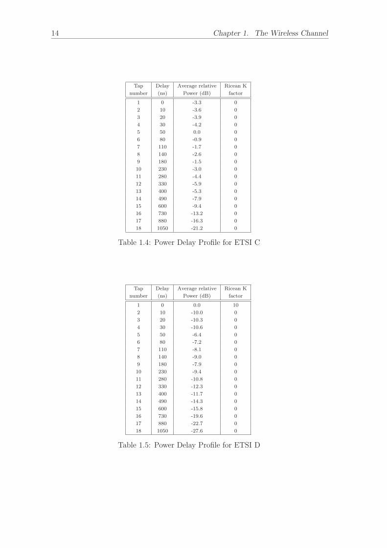
ETSI channel models As an example of propagation scenarios with NLOS com-
ponent the channel models by ETSI [6], [7] have been considered. Those models are
of reference for indoor wireless local area networks and imply an independent Jakes
Doppler spectrum on each tap. Summarizing, they and are characterized by:
• ETSI A: NLOS conditions and 50 ns average rms delay spread, corresponding
to a typical office environment;
• ETSI B: NLOS conditions and 100 ns average rms delay spread, corresponding
to a typical large open space and office environment;
• ETSI C: NLOS conditions and 150 ns average rms delay spread, corresponding
to a typical large open space;
• ETSI D: LOS conditions, same as ETSI C but with a 10 dB spike at zero delay
and 140 ns average rms delay spread;
• ETSI E: NLOS conditions and 250 ns average rms delay spread, corresponding
to a typical large open space.
The corresponding power delay profiles are reported in tables 1.2 to 1.6.

1.2. Wireless channel models 13
Tap Delay Average relative Ricean K
number (ns) Power (dB) factor
1 0 0.0 0
2 10 -0.9 0
3 20 -1.7 0
4 30 -2.6 0
5 40 -3.5 0
6 50 -4.3 0
7 60 -5.2 0
8 70 -6.1 0
9 80 -6.9 0
10 90 -7.8 0
11 110 -4.7 0
12 140 -7.3 0
13 170 -9.9 0
14 200 -12.5 0
15 240 -13.7 0
16 290 -18.0 0
17 340 -22.4 0
18 390 -26.7 0
Table 1.2: Power Delay Profile for ETSI A
Tap Delay Average relative Ricean K
number (ns) Power (dB) factor
1 0 -2.6 0
2 10 -3.0 0
3 20 -3.5 0
4 30 -3.9 0
5 50 0.0 0
6 80 -1.3 0
7 110 -2.6 0
8 140 -3.9 0
9 180 -3.4 0
10 230 -5.6 0
11 280 -7.7 0
12 330 -9.9 0
13 380 -12.1 0
14 430 -14.3 0
15 490 -15.4 0
16 560 -18.4 0
17 640 -20.7 0
18 730 -24.6 0
Table 1.3: Power Delay Profile for ETSI B
14 Chapter 1. The Wireless Channel
Tap Delay Average relative Ricean K
number (ns) Power (dB) factor
1 0 -3.3 0
2 10 -3.6 0
3 20 -3.9 0
4 30 -4.2 0
5 50 0.0 0
6 80 -0.9 0
7 110 -1.7 0
8 140 -2.6 0
9 180 -1.5 0
10 230 -3.0 0
11 280 -4.4 0
12 330 -5.9 0
13 400 -5.3 0
14 490 -7.9 0
15 600 -9.4 0
16 730 -13.2 0
17 880 -16.3 0
18 1050 -21.2 0
Table 1.4: Power Delay Profile for ETSI C
Tap Delay Average relative Ricean K
number (ns) Power (dB) factor
1 0 0.0 10
2 10 -10.0 0
3 20 -10.3 0
4 30 -10.6 0
5 50 -6.4 0
6 80 -7.2 0
7 110 -8.1 0
8 140 -9.0 0
9 180 -7.9 0
10 230 -9.4 0
11 280 -10.8 0
12 330 -12.3 0
13 400 -11.7 0
14 490 -14.3 0
15 600 -15.8 0
16 730 -19.6 0
17 880 -22.7 0
18 1050 -27.6 0
Table 1.5: Power Delay Profile for ETSI D

1.2. Wireless channel models 15
Tap Delay Average relative Ricean K
number (ns) Power (dB) factor
1 0 -4.9 0
2 10 -5.1 0
3 20 -5.2 0
4 40 -0.8 0
5 70 -1.3 0
6 100 -1.9 0
7 140 -0.3 0
8 190 -1.2 0
9 240 -2.1 0
10 320 0.0 0
11 430 -1.9 0
12 560 -2.8 0
13 710 -5.4 0
14 880 -7.3 0
15 1070 -10.6 0
16 1280 -13.4 0
17 1510 -17.4 0
18 1760 -20.9 0
Table 1.6: Power Delay Profile for ETSI E

16
Chapter 2
Orthogonal Frequency Division
Multiplexing
2.1 OFDM systems
Wireless channels in vehicular environment can exhibit high signal attenuation during
transmission and have a frequency-selective nature. In this scenario, if a single carrier
modulation system is used, channel equalization and data detection become difficult
tasks.
A popular wireless modulation technique is represented by orthogonal frequency
division multiplexing (OFDM). OFDM systems correspond to dividing the overall
information stream to be transmitted into many lower data rate streams, each one
modulating a different sub-carrier of the main frequency carrier. Equivalently, the
overall bandwidth is divided into many sub-bands centered on the sub-carriers. This
operation makes data communication more robust under wireless multi-path fading
channel and simplifies frequency equalization operations.
In the present chapter the filterless OFDM system with cyclic prefix extension
will also be introduced, which is used by many digital communication systems as
some standards of the IEEE 802.11 family, WiMax and the DVB Standard. The
particularity of this OFDM system is the efficient implementation and the simplicity
of equalization of the received symbol under frequency-selective wireless channel. A
complete treatment of OFDM systems can be found in [1].
An example of typical OFDM transmitter and receiver block diagrams are re-
ported in chapter 3, figures 3.4 and 3.5.
17

18 Chapter 2. Orthogonal Frequency Division Multiplexing
Figure 2.1: Block diagram of an OFDM system.
2.1.1 System model
In a OFDM system blocks of M complex symbols are transmitted in parallel over M
distinct sub-channels. The system block diagram is reported in figure 2.1. Let the
block of M symbols that are simultaneously transmitted at the given discrete time
instant kT be defined as
Ak = [Ak[0], Ak[1], . . . , Ak[M − 1]]T (2.1)
where each symbol Ak[i], i = 0, 1, . . . , M − 1, belongs to a two dimensional M-PSK
or M-QAM constellation Ai. The constellation cardinality could be different for
each sub-channel. Let the symbols Ak be zero mean and independent identically
distributed (i.i.d.). Moreover the constellation symbols are normalized in order to
get E [|A[i]|2] = 1, i = 0, 1, . . . , M − 1. The modulation rate is defined as F = 1/T
where T is the transmission period of the OFDM symbol Ak.
The i−th information data flow is zero padding interpolated by a factor M .
The time-resolution of the interpolated data-flow is Tc = T/M . Then the i−th
branch is filtered with a modulation filter cn[i] having impulse response given by
cn[i], n = 0, 1, . . . , Mq−1 and transfer function and frequency response respectively:
Ci(z) =+∞∑
n=−∞cn[i]z−n =
Mq−1∑n=0
cn[i]z−n (2.2)
Ci(f) = Ci(z)|z=ej2πfT/M , i = 0, 1, . . . , M − 1. (2.3)

2.1. OFDM systems 19
The filters used on the different sub-channels act as shaping filters for the M
upsampled branches. Note that the filters cn[i] work in parallel at rate Fc = 1/Tc =
M/T , where Tc = T/M is called transmission rate. The transmission bandwidth
of the system is given by B = 1/Tc = 1/(T/M) = M/T . The OFDM modulated
signal sn, that is transmitted over the wireless channel, is obtained by summing all
the resulting data flows
sn =M−1∑i=0
+∞∑
k=−∞Ak[i]cn−kM [i] (2.4)
With reference to the system shown in figure 2.1, the signal sn is transmitted
over the wireless channel that has impulse response given by
hk = [hk,0, hk,1, . . . , hk,Lch−1]T (2.5)
and transfer function Hk(z) defined as
Hk(z) =+∞∑
n=−∞hk,nz−n =
Lch−1∑n=0
hk,nz−n. (2.6)
The compact notation of the channel impulse response hk = h(kT ) takes into account
that, as furtherly discussed in section 3.1, in vehicular environment the wireless
channel can be considered static within one OFDM symbol time.
The AWGN noise wn has variance N0 and is the model for the thermal noise
generated ad the receiver. The block delay that introduces a delay of D0 time
instants, i.e. a delay time of D0Tc seconds, guarantes the proper synchronization at
the receiver side.
In case of ideal and noiseless channel, i.e. hk = [1, 0, 0, . . . , 0]T and wn = 0, it
results rn = sn.
At the receiver the received signal rn is filtered by M filters having impulse
responses given by gn[i] with support 0, 1, . . . , Mq− 1 and transfer function given
by
Gi(z) =+∞∑
n=−∞gn[i]z−n =
Mq−1∑n=0
gn[i]z−n (2.7)
for every i−th branch, i = 0, 1, . . . , M − 1. The M filters used by the demodula-
tor work in parallel at the transmission rate Fc. The output data flows are then
downsampled to the rate F = 1/T in order to achieve the reconstructed symbols
20 Chapter 2. Orthogonal Frequency Division Multiplexing
Yk[i], i = 0, 1, . . . ,M − 1. If the system composed by the cascade of modulator and
demodulator introduces a delay D0 in the signal reception, then the received vector
Yk = [Yk[0], Yk[1], . . . , Yk[M − 1]]T (2.8)
corresponds to the reconstruction of the OFDM symbol Ak−D0 transmitted D0 mod-
ulation intervals before.
Orthogonality Conditions With the assumption that the transmission is over
an ideal and noiseless channel, i.e. rn = sn, the transmission and reception filters
cn[i] and gn[i] are usually designed to satisfy a perfect reconstruction condition. This
mean that the designed filters have to guarantee:
• absence of inter-carrier interference (ICI); this means that no interference be-
tween symbols transmitted at the same time-instant on different sub-carriers
occurs;
• absence of inter-symbol interference (ISI); this means that no interference be-
tween symbols transmitted on the same sub-channel at different time-instants
occurs.
The support, in the time domain, of the filter cn[i] is indicated as 0, 1, . . . , Mq−1. Assuming matched filters are used at the receiver, i.e. gn[i] = c∗Mq−n[i], the
perfect reconstruction condition becomes [1]
Mq−1∑p=0
cp[i]gn−p[j] =
Mq−1∑p=0
cp[i]c∗Mq+p−n[j] =
=
Mq−1∑p=0
cp[i]c∗p+M(q−k)[j] =
= δi−jδk−q, i, j = 0, 1, . . . ,M − 1,
(2.9)
where δi,j is the Kronecker delta and n = Mq.
2.2 OFDM System with cyclic prefix
A simplified OFDM system implementation is now considered in which only one
prototype filter cn and gn is used for all sub-carriers respectively at the transmitter
and the receiver [1].
2.2. OFDM System with cyclic prefix 21
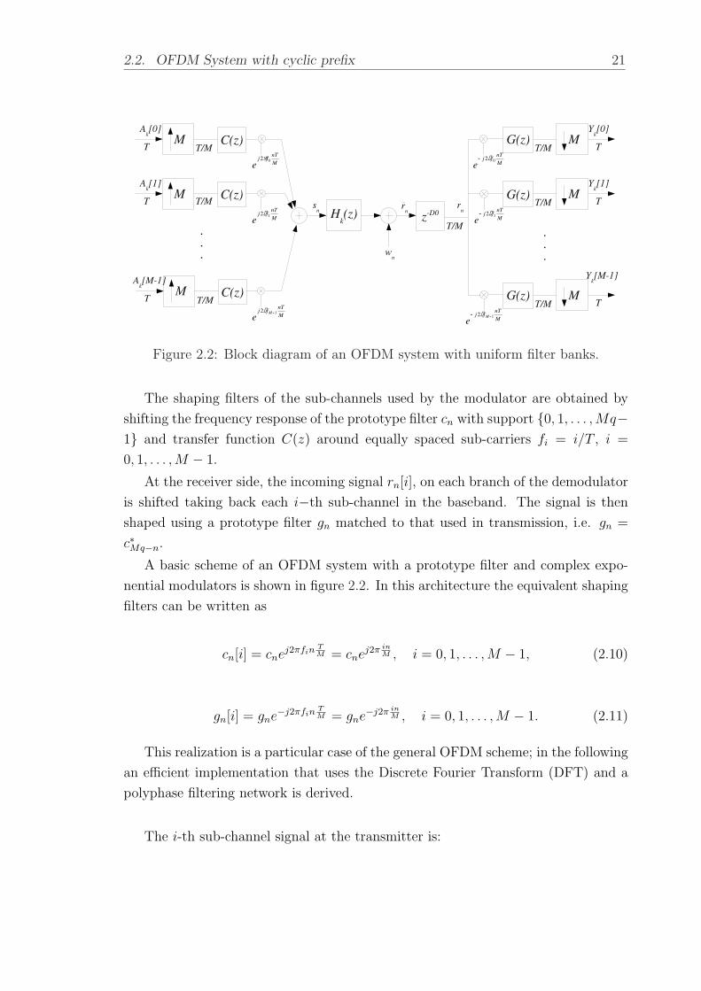
Figure 2.2: Block diagram of an OFDM system with uniform filter banks.
The shaping filters of the sub-channels used by the modulator are obtained by
shifting the frequency response of the prototype filter cn with support 0, 1, . . . , Mq−1 and transfer function C(z) around equally spaced sub-carriers fi = i/T , i =
0, 1, . . . , M − 1.
At the receiver side, the incoming signal rn[i], on each branch of the demodulator
is shifted taking back each i−th sub-channel in the baseband. The signal is then
shaped using a prototype filter gn matched to that used in transmission, i.e. gn =
c∗Mq−n.
A basic scheme of an OFDM system with a prototype filter and complex expo-
nential modulators is shown in figure 2.2. In this architecture the equivalent shaping
filters can be written as
cn[i] = cnej2πfinTM = cnej2π in
M , i = 0, 1, . . . ,M − 1, (2.10)
gn[i] = gne−j2πfinTM = gne−j2π in
M , i = 0, 1, . . . , M − 1. (2.11)
This realization is a particular case of the general OFDM scheme; in the following
an efficient implementation that uses the Discrete Fourier Transform (DFT) and a
polyphase filtering network is derived.
The i-th sub-channel signal at the transmitter is:
22 Chapter 2. Orthogonal Frequency Division Multiplexing
sn[i] = ej2π inM
+∞∑
k=−∞Ak[i]cn−kM (2.12)
and the overall signal sn:
sn =M−1∑i=0
ej2π inM
+∞∑
k=−∞cn−kMAk[i]. (2.13)
With the change of variables n = mM + l with l = 0, . . . , M − 1, it turns that:
smM+l =M−1∑i=0
ej2π iM
(mM+l)
+∞∑
k=−∞c(m−k)M+lAk[i]. (2.14)
It should be noted that ej2πim = 1. By expressing the l−th polyphase components
of smM+l and cmM+l as
s(l)m = smM+l (2.15)
and
c(l)m = cmM+l, (2.16)
the l-th polyphase component of sn results:
s(l)m =
+∞∑
k=−∞c(l)m−k
M−1∑i=0
W−ilM Ak[i] (2.17)
where c(l)m , l = 0, 1, . . . , M−1 denotes the polyphase component of the prototype filter
impulse response with related transfer function defined as C(l)(z) and WM = e−j 2πM .
The inner summation in (2.17) is:
M−1∑i=0
W−ilM Ak[i] = ak[l], l = 0, 1, . . . , M − 1 (2.18)
being ak[l] the l−th element of the IDFT of Ak ∈ CM×1, defined as ak = F−1M Ak,
with l = 0, 1, . . . , M − 1.
Finally the l-th polyphase component of sn can be expressed as:
s(l)n =
+∞∑
k=−∞c(l)n−kak[l] =
+∞∑p=−∞
c(l)p an−p[l]. (2.19)
2.2. OFDM System with cyclic prefix 23
From this relation it follows that each sample of the signal sn can be obtained by
the convolution of the signal at the l−th output of the IDFT block with the l−th
polyphase component of the prototype filter c(l)n .
With reference to the figure 2.2, at the receiver side the relation between the
received sequence rn = rn−D0 and the output of the i-th sub-channel Yk[i] is:
Yk[i] =+∞∑
n=−∞rngkM−ne−j2πfin
TM =
+∞∑n=−∞
rngkM−ne−j2π in
M . (2.20)
With the change of variables n = mM + l, l = 0, 1, . . . ,M − 1 and recalling the
definition of matched filter gn = c∗Mq−n, it reads
Yk[i] =M−1∑
l=0
+∞∑m=−∞
c∗(q−k+m)M+le−j2π i
M(mM+l)rmM+l. (2.21)
We further note that e−j2πim = 1 and set r(l)m = rmM+l, c
(l)∗m = c∗mM+l, so the
output signal can be written as:
Yk[i] =M−1∑
l=0
e−j 2πM
il
+∞∑m=−∞
c(l)∗q+m−kr
(l)m (2.22)
that finally becomes, employing the relation e−j 2πM
il = W ilM ,
Yk[i] =M−1∑
l=0
W ilM
+∞∑m=−∞
c(l)∗q+m−kr
(l)m . (2.23)
The demodulator can be implemented using a bank of polyphase filters, where for
each l−th branch, l = 0, 1, . . . , M −1, the content of the delay line is convolved with
the l−th polyphase component g(l)m of the matched filter gk.
The resulting scheme comprising a inverse DFT (IDFT) operation at the trans-
mitter and a DFT operation at the receiver is shown in figure 2.3. It should be noted
that the rate of the equivalent shaping filters c(l)m and g
(l)m is T and the upsampling
operation to the transmission rate Tc = T/M is obtained with the P/S operation
on the M polyphase components s(l)m of the output signal sn. Moreover, as matched
filters g(l)m are used, their respective transfer functions read G(l)(z) = C(l)∗(1/z∗).

24 Chapter 2. Orthogonal Frequency Division Multiplexing
Figure 2.3: Block diagram of an OFDM system with efficient implementation.
2.2.1 Equalization in OFDM systems
In the present section the filterless OFDM system implementation is derived. The
filterless OFDM system is a system where the prototype filters used at transmitter
and receiver are given by
cn =
1 0 ≤ n ≤ M − 1
0 otherwise(2.24)
The impulse response of the polyphase components of the prototype filter are:
c(l)n
= δn l = 0, 1, . . . M − 1. (2.25)
This assumption satisfies the orthogonality conditions (2.9). It results that the
transmitted signal can be obtained by directly applying the P/S conversion at the
output of the IDFT.
Under the condition of ideal and noiseless channel, at the receiver the S/P con-
verter creates block of M samples so that the output of the IDFT goes unchanged
to the input of the DFT and the output produces the transmitted signal without
distortion.
A channel having impulse response hk, transfer function Hk(z) and support
0, 1, . . . , Lch− 1, with Lch > 1 is considered. The equalization technique is simpli-
fied if the concept of circular convolution can be applied, that allows expressing the
convolution between two discrete-time sequences in the time domain as the product
of finite length between the DFT of the same sequences [1].

2.2. OFDM System with cyclic prefix 25
Figure 2.4: Block diagram of a filterless OFDM system with cyclic prefix and
frequency-domain equalizer.
In order to enable circular convolutions, with reference to figure 2.4, the block
of symbols ak is extended appending the last Lcp − 1 = Lch − 1 elements at the
beginning of the sequence. In this way for the same transmission rate M/T the
IDFT must work at the rate 1T ′ = M
(M+Lcp−1)T< 1
T. After the P/S conversion, the
Lcp− 1 + M samples are transmitted over the channel. At the receiver the blocks of
Lcp− 1+M samples are obtained after the S/P conversion; the first Lcp− 1 samples
are discarded prior to DFT operations.
Beware of the properties of circular convolution, the vector rk of the last M
samples of the block received at time instant kT is given by:
rk = Λkhk + wk (2.26)
where hk = [hk,0, . . . , hk,Lch−1, 0, . . . , 0]T is the M -component vector of the channel
impulse response extended with M − Lch zeros, wk is the AWGN vector and Λk is
the M ×M circulant matrix of the transmitted symbol, defined as:
Λk =
ak[0] ak[M − 1] · · · ak[1]
ak[1] ak[0] · · · ak[2]...
.... . .
...
ak[M − 1] ak[M − 2] · · · ak[0]
. (2.27)
26 Chapter 2. Orthogonal Frequency Division Multiplexing
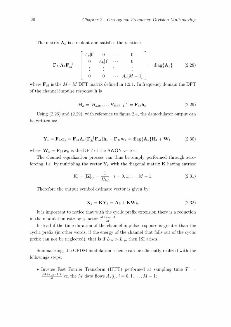
The matrix Λk is circulant and satisfies the relation:
FMΛkF−1M =
Ak[0] 0 · · · 0
0 Ak[1] · · · 0...
.... . .
...
0 0 · · · Ak[M − 1]
= diagAk (2.28)
where FM is the M×M DFT matrix defined in 1.2.1. In frequency domain the DFT
of the channel impulse response h is
Hk = [Hk,0, . . . , Hk,M−1]T = FMhk. (2.29)
Using (2.26) and (2.29), with reference to figure 2.4, the demodulator output can
be written as:
Yk = FMrk = FMΛk(F−1M FM)hk + FMwk = diagAkHk + Wk (2.30)
where Wk = FMwk is the DFT of the AWGN vector.
The channel equalization process can thus be simply performed through zero-
forcing, i.e. by multipling the vector Yk with the diagonal matrix K having entries:
Ki = [K]i,i =1
Hk,i
i = 0, 1, . . . , M − 1. (2.31)
Therefore the output symbol estimate vector is given by:
Xk = KYk = Ak + KWk. (2.32)
It is important to notice that with the cyclic prefix extension there is a reduction
in the modulation rate by a factor M+Lcp−1
M.
Instead if the time duration of the channel impulse response is greater than the
cyclic prefix (in other words, if the energy of the channel that falls out of the cyclic
prefix can not be neglected), that is if Lch > Lcp, then ISI arises.
Summarizing, the OFDM modulation scheme can be efficiently realized with the
followings steps:
• Inverse Fast Fourier Transform (IFFT) performed at sampling time T ′ =(M+Lcp−1)T
Mon the M data flows Ak[i], i = 0, 1, . . . , M − 1;

2.2. OFDM System with cyclic prefix 27
• appending the last Lcp − 1 samples of the data block at the beginning of the
block as cyclic prefix;
• parallel to serial conversion (P/S) of the resulting M data flows, which is
essentially a time division multiplexer.
Moreover an efficient digital implementation of the OFDM demodulator consists
of:
• a serial to parallel (S/P) block that let a sequence of M + Lcp − 1 consecutive
samples of the received signal be input on M + Lcp − 1 lines;
• the cyclic prefix removal obtained by eliminating the first Lcp − 1 symbols of
every data block.
• a Fast Fourier Transform (FFT) performed at sampling time T to the sym-
bols rn[i], i = 0, 1, . . . , M − 1 to obtain the demodulated symbols Yk[i], i =
0, 1, . . . ,M − 1;
• a zero-forcing equalization of the demodulated symbols Yk[i] as reported in
(2.31) and (2.32) to obtain the symbol estimates to be used for the data de-
tection.

28

Chapter 3
IEEE 802.11p Standard for WLAN
in Vehicular Environment
3.1 Introduction
Vehicle to vehicle (V2V) and vehicle to roadside-unit (RSU) communications (known
as vehicle to infrastructure, V2I) represent a promising technology to support Intel-
ligent Transportation Systems (ITS) applications. An official classification of ITS
applications does not exist. However, potentially a vast set of applications can be
provided, ranging from driver safety increase, which is the main purpose of these
networks, to traffic flow monitoring and congestion mitigation, or electronic tolling
collection. A possible scenario is shown in figure 3.1.
Dedicated Short Range Communications (DSRC) is the communication standard
for general purpose V2V and V2I RF communication links. More specifically, it is a
short to medium range communication service that supports several applications (like
public safety, or electronic toll collection) requiring very low latency and high data
rate. Concerning the physical layer (PHY) of DSRC technologies, most standards
under development in different countries worldwide will be based on IEEE 802.11p
[3], which is an amendment of the family of IEEE 802.11 standards for wireless local
area network (WLAN) communications, both for physical layer and medium access
control (MAC) layer, that introduces a set of specifications to enable Wireless Access
in Vehicular Environment (in short, WAVE).
WAVE technology aims to guarantee wireless connectivity to IEEE 802.11 devices
in vehicular environments where the physical layer properties are rapidly changing
29

30 Chapter 3. IEEE 802.11p Standard for WLAN in Vehicular Environment
and where very short-duration communications exchanges are required. The pur-
pose of IEEE 802.11p is then to provide the minimum set of specifications required
to ensure interoperability between wireless devices attempting to communicate in
potentially rapidly changing communication environments and in situations where
transactions must be completed in time frames much shorter than the minimum
possible with infrastructure or ad hoc 802.11 networks. At the time of writing the
standard is nearly finalized and final approval is expected by the end of 2010.
IEEE 802.11p physical layer is very similar to the popular IEEE 802.11a/g stan-
dards, OFDM-based, with the main differences being represented by the use of 5.9
GHz range (5.85-5.925 GHz) instead of 5.2 of the latter, and by the addition of a
reduced bandwidth (10 MHz instead of 20 MHz).
There are however some difficulties, from a PHY perspective, of applying IEEE
802.11 to mobile communications systems, related to the perturbation of the signal
due to the radio channel.
The outdoor propagation environment is generally characterized by longer delay
spreads than indoor channels because the propagating radio signal is subject to obsta-
cles such as buildings and trees, which can lead to strong reflective and/or diffractive
multi-path effects placed at larger distances among them than in indoor environment.
As a result, interference from the previously transmitted OFDM symbol, i.e. ISI can
more easily arise for an outdoor environment than for indoor environments. It should
be noticed that the bandwidth reduction of IEEE 802.11p compared to IEEE 802.11
a/g translates in a longer guard interval (GI) duration so to cope with the higher
multi-path effect of urban environments.
3.2 IEEE 802.11p Physical layer
3.2.1 General description
IEEE 802.11p operates in the Dedicated Short Range Communications band allo-
cated for Intelligent Transportation Systems (ITS) applications. They can occur
between mobile stations and fixed information sources, between mobile units, and
between portable units and mobile units. Transmissions have to be guaranteed over
line-of-sight (LOS) between fixed and mostly high-speed units. They can also occur
between stopped and slow moving vehicles, or between high-speed vehicles.
IEEE 802.11p standard specifications [3] include:

3.2. IEEE 802.11p Physical layer 31
Figure 3.1: Example of V2V and V2I communications
• description of the functions and services required by WAVE-conformant sta-
tions in order to operate in vehicular environment and exchange messages with-
out having to join a set of station clients (STAs) controlled by an Access Point
(AP);
• definition of the WAVE signalling technique and interface functions that are
controlled by the IEEE 802.11 Medium Access Control (MAC).
Physical layer specifications WAVE PHY is based on OFDM modulation. The
radio frequency LAN system operates in the [5.850- 5.925] GHz frequency band, and
7 channels each 10 MHz wide are provided. In particular, one of them is dedicate
to control functions, while the others are service channels. Optionally, 2 pairs of
adjacent channels may be merged together in order to obtain two channels of 20
MHz.
The OFDM system provides a WLAN with 10 MHz bandwidth and data payload
communication capabilities of 3, 4.5, 6, 9, 12, 18, 24 and 27 Mbit/s. In particular the
support to transmitting and receiving data rates of 3, 6 and 12 Mbit/s is mandatory.
Optionally, support for 20 MHz bandwidth can be granted and related data rates
of 6, 9, 12, 18, 24, 36, 48 and 54 Mbit/s are provided. The OFDM system uses
52 sub-carriers that are modulated using binary or quadrature phase shift keying
(BPSK,QPSK), 16-quadrature amplitude modulation (QAM), and 64-QAM. More-

32 Chapter 3. IEEE 802.11p Standard for WLAN in Vehicular Environment
Transmission Modulation Coding Coded Coded bits Data bitsrate [MHz] rate bits per per ODFM per OFDM
sub-carrier symb. symb.(NBPSC) (NCPSC) (NDPSC)
3 BPSK 1/2 1 48 24
4.5 BPSK 3/4 1 48 36
6 QPSK 1/2 2 96 48
9 QPSK 3/4 2 96 72
12 16-QAM 1/2 4 192 96
18 16-QAM 3/4 4 192 144
24 64-QAM 2/3 6 288 192
27 64-QAM 3/4 6 288 216
Table 3.1: Transmission rates, B = 10 MHz
over forward error correction coding with 64-state convolutional code is used with
code rates of 1/2, 2/3, or 3/4, as it is shown in tables 3.1 and 3.2.
3.2.2 OFDM parameters
In the following the main OFDM parameters of IEEE 802.11p are recalled. Table
3.3 reports the main parameters of the OFDM system for the two configurations of
10 and 20 MHz. The parameters reported in table 3.3 are defined as:
• T : OFDM symbol period (after cyclic prefix extension);
• Tc: chip time, corresponding to the discrete sampling time after the OFDM
modulation;
• Ts: block symbol period, corresponding to the OFDM symbol duration without
cyclic prefix;
• Tcp: cyclic prefix duration;
• Lcp: cyclic prefix length, expressed in number of modulated symbols.
Table 3.4 reports the sub-carriers repartition between data, virtual and pilot sub-
carriers: data sub-carriers modulate the transmitted data, virtual sub-carriers are
not used in the data transmission to achieve better out-of band signal reduction and

3.2. IEEE 802.11p Physical layer 33
Transmission Modulation Coding Coded Coded bits Data bitsrate [MHz] rate bits per per ODFM per OFDM
sub-carrier symb. symb.(NBPSC) (NCPSC) (NDPSC)
6 BPSK 1/2 1 48 24
9 BPSK 3/4 1 48 36
12 QPSK 1/2 2 96 48
18 QPSK 3/4 2 96 72
24 16-QAM 1/2 4 192 96
36 16-QAM 3/4 4 192 144
48 64-QAM 2/3 6 288 192
54 64-QAM 3/4 6 288 216
Table 3.2: Transmission rates, B = 20 MHz
Parameter B = 10 MHz B = 20 MHz
Sampling time 100 ns 50 ns
Frequency spacing 156.25 kHz 312.5 kHz
between sub-carriers
T 8 µs 4 µs
Tc 0.1 µs 0.05 µs
Ts 6.4 µs 3.2 µs
Tcp 1.6 µs 0.8 µs
Lcp 16 16
Table 3.3: Parameters of the OFDM system in IEEE 802.11p
pilot sub-carriers modulate symbols known at the receiver in order to perform the
CE tasks (see section 5.2).
3.2.3 Frame structure
The PHY layer consists of two sub-layers:
1. the physical layer convergence procedure (PLCP) sub-layer defines a method
of mapping the IEEE 802.11 PHY sub-layer service data units (PSDU) into
a PHY packet, of a format suitable for sending and receiving user data and
management information between two or more stations using the associated

34 Chapter 3. IEEE 802.11p Standard for WLAN in Vehicular Environment
Type of sub-carriers n. index
Total 64 1,. . . ,64
Virtual sub-carriers 12 1, 28, . . . , 38
Pilot sub-carriers 4 8, 22, 44, 58
Data sub-carriers 48 2, . . . , 7, 9, . . . , 21, 23, . . . , 27,
39, . . . , 43, 45, . . . , 57, 59, . . . , 64
Table 3.4: Sub-carrier indexes for IEEE 802.11p
Figure 3.2: Schematic representation of PHY and MAC layers of IEEE 802.11p
physical medium dependent (PMD) system. This procedure is called the PHY
convergence function, offered by the PHY layer. In this way the IEEE 802.11
MAC layer operates with minimum dependence on the PMD sub-layer;
2. a PMD system whose function defines the characteristics and methods of trans-
mitting and receiving data through a wireless medium between two or more
stations. The service of a layer or sub-layer is the set of capabilities that it
offers to a user in the next higher layer. In this case the PHY services are
offered to the MAC sub-layer, which is intended to be PHY independent.
The PLCP sub-layer converts a PHY sub-layer service data unit (PSDU) to a
PLCP protocol data unit (PPDU), and a PPDU to a PSDU. In transmission, the
PSDU received from the MAC sub-layer shall be provided with a PLCP preamble

3.2. IEEE 802.11p Physical layer 35
and header to create the PPDU. At the receiver, the PLCP preamble and header
of the PPDU are processed to aid the demodulation and the delivery of the PSDU.
The structure of the PHY layer is shown in figure 3.2.
PLCP frame format The PLCP frame is composed of the OFDM PLCP pream-
ble, the OFDM PLCP header, the PSDU provided by the MAC, tail bits, and pad
bits as shown in figure 3.3. The PLCP preamble is used for synchronization, the
PLCP header contains informations used for the correct interpretation of data as
the fields LENGTH and RATE, the PSDU unit contains the transmitted data pay-
load.
PLCP preamble At the receiver, the preamble is used for the synchronization
task. In IEEE 802.11p the PLCP preamble is composed of a short training sequence
(STS) composed of 10 short training symbols t1, · · · , t10 and a long training sequence
(LTS) composed by two OFDM symbols. Both STS and LTS are known at the
receiver. The total training length is 16µs and 32µs respectively if the bandwidth is
B = 20 MHz or B = 10 MHz.
During STS reception Automatic gain control (AGC) and signal detection are
performed, they are usually completed after a random time. Then, the STS can be
only partially exploited for the synchronization task. Typically the first 4 or 5 short
training symbols are not available for the system synchronization. A short OFDM
training symbol consists of 12 sub-carriers, which are modulated by the elements of
the sequence S, given by
S1,52 =√
13/60, 0, 1 + j, 0, 0, 0,−1− j, 0, 0, 0, 1 + j, 0, 0, 0,−1− j,
0, 0, 0,−1− j, 0, 0, 0, 1 + j, 0, 0, 0, 0, 0, 0, 0,−1− j, 0, 0, 0,−1− j, 0,
0, 0, 1 + j, 0, 0, 0, 1 + j, 0, 0, 0, 1 + j, 0, 0, 0, 1 + j, 0, 0 (3.1)
where the factor√
13/6 is used to normalize the average power of the resulting
OFDM symbol, which utilizes 12 out of 52 sub-carriers. Each short training symbol
has a duration of 0.8µs if the bandwidth is B = 20 MHz or 1.6µs if the bandwidth
is B = 10 MHz.
The two OFDM training symbols that compose the LTS are used to perform
CE and to improve synchronization accuracy. The two long training symbols are

36 Chapter 3. IEEE 802.11p Standard for WLAN in Vehicular Environment
Figure 3.3: IEEE 802.11p packet frame, c©IEEE 1999.
obtained using all 52 data sub-carriers, which are modulated by the elements of the
sequence L, given by
L1,52 = 1, 1,−1,−1, 1, 1,−1, 1,−1, 1, 1, 1, 1, 1, 1,−1,−1, 1, 1,−1,
1,−1, 1, 1, 1, 1, 1,−1,−1, 1, 1,−1, 1,−1, 1,−1,−1,−1,−1,−1, 1, 1,−1,
− 1, 1,−1, 1,−1, 1, 1, 1, 1 (3.2)
The total duration of the LTS is TLTS = 2 ∗ 1.6+2 ∗ 6.4 = 16µs if the bandwidth
is B = 10 MHz, where 1.6µs is the duration of the GI added to the LTS symbols as
shown in figure 3.3.
PLCP header and PSDU structure In the PLCP header are included several
fields to be used for the correct interpretation of data. It contains the following
fields: LENGTH, RATE, a reserved bit, an even parity bit, and the SERVICE field.
The RATE and LENGTH fields, reserved bit, and parity bit (with 6 zero tail bits
appended) constitute the symbol called SIGNAL. It is one OFDM symbol of length
M = 64 that is cyclically extended with a GI of length Lcp = 16, and it is transmitted
with the most robust combination of BPSK modulation and a coding rate of 1/2.
The SERVICE field and the PSDU, which are denoted as DATA, are transmitted
at the data rate described in the RATE field. They may be composed by multiple
OFDM consecutive symbols, and each symbol is cyclically extended with a guard
interval. SERVICE is a 16 bit field. The first six bits are set to zero, and they
are used to synchronize the descrambler at receiver. The remaining 9 bits shall be
reserved for future use.
The PPDU tail bit field contains six zero bits. With this field the convolutional
encoder can return to the zero state. This procedure can improve the error prob-

3.2. IEEE 802.11p Physical layer 37
Figure 3.4: Block diagram of the IEEE 802.11p transmitter
Figure 3.5: Block diagram of the IEEE 802.11p receiver
ability of the convolutional decoder, which relies on future bits when decoding and
which may be not be available past the end of the message [3].
The number of bits in the DATA field has to be a multiple of the number of coded
bits in an OFDM symbol, that is 48, 96, 192, or 288 bits as shown in tables 3.1 and
3.2. The length of the message is then extended in order to become a multiple of the
number of data bits per OFDM symbol. The tail bits are always appended to the
message, and thus and the number of padding bits are computed taking into account
the PSDU length.
PPDU generation process The PPDU generation process is summarized below
through the following steps as described in [4]. The transmitter and receiver block
diagrams are shown in figures 3.4 and 3.5.
(a) Produce the PLCP preamble made of the ten repetitions of the STS and two
repetitions of the LTS preceded by a GI as described above.
(b) Generate the PLCP header field with the RATE, LENGTH, and SERVICE fields.
Encode the SIGNAL field with the convolutional encoder with rare 1/2, per-
form interleaving, BPSK modulation, pilot insertion, Fourier transform, and
pre-pending a GI. The content of the SIGNAL field is not scrambled.
38 Chapter 3. IEEE 802.11p Standard for WLAN in Vehicular Environment
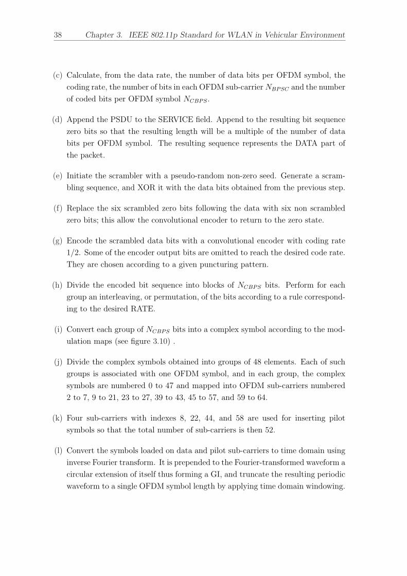
(c) Calculate, from the data rate, the number of data bits per OFDM symbol, the
coding rate, the number of bits in each OFDM sub-carrier NBPSC and the number
of coded bits per OFDM symbol NCBPS.
(d) Append the PSDU to the SERVICE field. Append to the resulting bit sequence
zero bits so that the resulting length will be a multiple of the number of data
bits per OFDM symbol. The resulting sequence represents the DATA part of
the packet.
(e) Initiate the scrambler with a pseudo-random non-zero seed. Generate a scram-
bling sequence, and XOR it with the data bits obtained from the previous step.
(f) Replace the six scrambled zero bits following the data with six non scrambled
zero bits; this allow the convolutional encoder to return to the zero state.
(g) Encode the scrambled data bits with a convolutional encoder with coding rate
1/2. Some of the encoder output bits are omitted to reach the desired code rate.
They are chosen according to a given puncturing pattern.
(h) Divide the encoded bit sequence into blocks of NCBPS bits. Perform for each
group an interleaving, or permutation, of the bits according to a rule correspond-
ing to the desired RATE.
(i) Convert each group of NCBPS bits into a complex symbol according to the mod-
ulation maps (see figure 3.10) .
(j) Divide the complex symbols obtained into groups of 48 elements. Each of such
groups is associated with one OFDM symbol, and in each group, the complex
symbols are numbered 0 to 47 and mapped into OFDM sub-carriers numbered
2 to 7, 9 to 21, 23 to 27, 39 to 43, 45 to 57, and 59 to 64.
(k) Four sub-carriers with indexes 8, 22, 44, and 58 are used for inserting pilot
symbols so that the total number of sub-carriers is then 52.
(l) Convert the symbols loaded on data and pilot sub-carriers to time domain using
inverse Fourier transform. It is prepended to the Fourier-transformed waveform a
circular extension of itself thus forming a GI, and truncate the resulting periodic
waveform to a single OFDM symbol length by applying time domain windowing.

3.2. IEEE 802.11p Physical layer 39
Figure 3.6: Data scrambler
(m) Concatenate the OFDM data symbols one after the other, starting after the
SIGNAL symbol describing the RATE and LENGTH.
(n) Up-convert the complex baseband waveform obtained to an RF frequency ac-
cording to the center frequency of the desired channel and transmit.
3.2.4 Scrambling, coding, interleaving and mapping
In the following the procedures of scrambling, encoding, interleaving and mapping
for the SIGNAL and DATA symbols for IEEE 802.11p will be described.
Scrambler A scrambler is a device that transposes or inverts bits, or, otherwise,
encodes a bit sequence, at the transmitter to make the message unintelligible at any
receiver that is not equipped with the appropriately descrambling device.
The DATA field of the PHY packet shall be scrambled with a length-127 frame-
synchronous scrambler [3]. Octets of the PSDU are placed in the transmit serial bit
stream, bit 0 in the first position and bit 7 as last. The frame synchronous scrambler
uses the following generator polynomial
S(x) = x7 + x4 + 1 (3.3)
and the 127-bit sequence cyclically generated shall be (leftmost used first)
00001110 11110010 11001001 00000010 00100110 00101110 10110110 00001100
11010100 11100111 10110100 00101010 11111010 01010001 10111000 1111111,
(3.4)
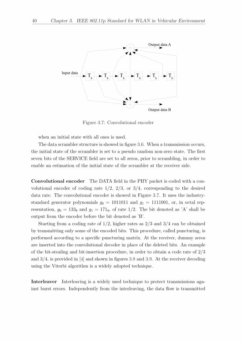
40 Chapter 3. IEEE 802.11p Standard for WLAN in Vehicular Environment
Figure 3.7: Convolutional encoder
when an initial state with all ones is used.
The data scrambler structure is showed in figure 3.6. When a transmission occurs,
the initial state of the scrambler is set to a pseudo random non-zero state. The first
seven bits of the SERVICE field are set to all zeros, prior to scrambling, in order to
enable an estimation of the initial state of the scrambler at the receiver side.
Convolutional encoder The DATA field in the PHY packet is coded with a con-
volutional encoder of coding rate 1/2, 2/3, or 3/4, corresponding to the desired
data rate. The convolutional encoder is showed in Figure 3.7. It uses the industry-
standard generator polynomials g0 = 1011011 and g1 = 1111001, or, in octal rep-
resentation, g0 = 1338 and g1 = 1718, of rate 1/2. The bit denoted as ’A’ shall be
output from the encoder before the bit denoted as ’B’.
Starting from a coding rate of 1/2, higher rates as 2/3 and 3/4 can be obtained
by transmitting only some of the encoded bits. This procedure, called puncturing, is
performed according to a specific puncturing matrix. At the receiver, dummy zeros
are inserted into the convolutional decoder in place of the deleted bits. An example
of the bit-stealing and bit-insertion procedure, in order to obtain a code rate of 2/3
and 3/4, is provided in [4] and shown in figures 3.8 and 3.9. At the receiver decoding
using the Viterbi algorithm is a widely adopted technique.
Interleaver Interleaving is a widely used technique to protect transmissions aga-
inst burst errors. Independently from the interleaving, the data flow is transmitted

3.2. IEEE 802.11p Physical layer 41
Figure 3.8: Puncturing procedure for rate R = 3/4, c©IEEE 1999.
with some redundant bits obtained after encoding that enable the decoder to correct
a given number of altered bits, depending on the error-correcting code used. If a
burst error occurs, resulting in a number of altered bits that is greater than the
correction capability of the code, then the codeword can not be correctly decoded.
In [3], the interleaver is defined by two permutations, and all the encoded data
bits provided by the convolutional encoder are interleaved by a block interleaver with
a block size corresponding to the number of coded bits in a single OFDM symbol,
NCBPS. The first permutation of the interleaver guarantees that adjacent coded bits
are mapped onto nonadjacent sub-carriers. The second ensures that adjacent coded
bits are mapped alternately onto less and more significant bits of the constellation
and, thereby, long runs of low reliability bits are avoided.
Let k be the index of the coded bit before the first permutation, i the index
after the first and before the second permutation and j the index after the second
permutation, just prior to modulation mapping. The first permutation is defined by
the rule:

42 Chapter 3. IEEE 802.11p Standard for WLAN in Vehicular Environment
Figure 3.9: Puncturing procedure for rate R = 2/3, c©IEEE 1999.
i =NCBPS
16(k mod 16) +
⌊k
16
⌋, k = 0, 1, . . . , NCBPS − 1 (3.5)
and the second is defined by
j = s ·⌊
i
s
⌋+
(i + NCBPS −
⌊16
i
NCBPS
⌋)mod s, i = 0, 1, . . . , NCBPS−1 (3.6)
where NBPSC is the number of coded bits per sub-carrier and s is given by
s = max(NBPSC/2, 1).
The deinterleaver performs the inverse operation, also composed of two steps.
Here, let j be the index of the received bit before the first permutation, i the index
between the permutations, and k the index after the second permutation, before the
coded bits are passed to the convolutional decoder. The first permutation is:
i = s ·⌊
j
s
⌋+
(j +
⌊16
j
NCBPS
⌋)mod s, j = 0, 1, . . . , NCBPS − 1 (3.7)
where s is given by s = max(NBPSC/2, 1) and the second permutation is:

3.2. IEEE 802.11p Physical layer 43
Modulation KMOD
BPSK 1
QPSK 1/√
2
16-QAM 1/√
10
64-QAM 1/√
42
Table 3.5: Modulation dependent normalization factor
k = 16 · i− (NCBPS − 1)
⌊16
i
NCBPS
⌋i = 0, 1, . . . , NCBPS − 1 (3.8)
Subcarrier modulation mapping The encoded and interleaved bits are divided
into groups of NBPSC bits (equal to 1, 2, 4, or 6 as shown in Table 3.1) and converted
into complex symbols representing BPSK, QPSK, 16-QAM, or 64-QAM constellation
points. The modulation type is chosen depending on the requested transmission rate.
The conversion into the constellation symbols is performed according to Gray-coded
mapping as illustrated in figure 3.10. In order to obtain an equal average power for all
mappings, the complex constellation points (I+jQ) are multiplied by a normalization
factor KMOD. The output values, B, are given by
B = (I + jQ)×KMOD (3.9)
where KMOD depends on the modulation and can assume the values reported in
table 3.5.

44 Chapter 3. IEEE 802.11p Standard for WLAN in Vehicular Environment
Figure 3.10: PSK, QPSK, 16-QAM, and 64-QAM constellation bit encoding, c©IEEE
1999.

3.2. IEEE 802.11p Physical layer 45
Parameter supported values
Bandwidth B 10, 20 MHz
Data rates 3, . . . , 27 Mbps (for B = 10 MHz)6, . . . , 54 Mbps (for B = 20 MHz)
Channel model ETSI A, B, C, D, E with Jakes Doppler
CIR length ideal knowledge or estimated
Channel estimation ideal, TD-LS, TD-LS RR, modified-RR
DDCE ideal, no tracking,iterative FEC aided, non-iterative FEC aided
Table 3.6: Simulator supported options
3.2.5 Implemented MATLAB model of IEEE 802.11p
The analysis and simulations presented in the following chapters have been obtained
with a MATLAB chain that implements the last draft version of the IEEE 802.11p
standard [3].
The simulator implements:
• the equivalent baseband transmitter compliant with [3] as described in the
previous section; in particular the whole set of data rates available in IEEE
802.11p is supported;
• the discrete-time wireless channel simulator, in particular the ETSI models with
Doppler effect presented in section 1.2.2 for the equivalent baseband discrete
time-varying frequency selective wireless channel have been implemented;
• the equivalent baseband receiver as shown in the block diagram of figure 3.5
with perfect and real timing and frequency synchronizations. Moreover ideal
and several real CE options have been modeled; these estimation algorithms
are described in more details in section 4.1;
• the addition of the decision directed CE algorithms described in chapter 5.
The supported simulator options are summarized in table 3.6. Other important
simulation parameters that can be specified by the user are: packet length, relative
speed, SNR at the receiver, frequency offset.

46
Chapter 4
Channel estimation algorithms for
OFDM systems
4.1 Channel estimation algorithms
The previous chapters reported a description of the wireless channel theory and the
OFDM systems and the related equalization techniques, described assuming CIR
(or equivalently CFR) known at the receiver. The CIR must be estimated in real
systems.
This chapter describes a summary of the main channel estimation (CE) algo-
rithms for OFDM systems.
The CE algorithms for OFDM systems can be divided into two main classes:
• Blind techniques, that are based only on the received data and statistically
estimate the channel behavior without any further knowledge;
• non-blind techniques, which perform the CE task using the knowledge of pre-
vious channel estimations or some portion of transmitted data.
Blind algorithms The blind estimation techniques typically perform the CE by
considering the second order statistics of the received data without any a priori
knowledge of pilot symbols or previous channel estimates. Their main advantage is
their high spectral efficiency, because there is no need to transmit extra data symbols
for training purpose. The main drawback is the estimation long convergence time
because of the long time required to achieve reliable estimated second order statistics
of the received data [9], [10].
47
48 Chapter 4. Channel estimation algorithms for OFDM systems
Non-blind algorithms The non-blind CE techniques exploit the knowledge at
the receiver of ad-hoc transmitted data such as pilot symbols or training sequences.
The a-priori knowledge of given transmitted data sequences makes the estimation
task easier and faster than the blind approach. The main drawback is the consequent
reduction of the spectral efficiency.
In literature semi-blind algorithms are also present; they make simultaneously
use of both blind and non-blind approaches: in [11] a periodic sequence of pilot
symbols and the first-order statistic of the time-domain received symbols are used
to estimate the frequency-selective channel in OFDM systems.
Popular wireless OFDM applications foresee the transmission of a “preamble”
composed of proper training sequences for CE purpose. This is also the case of
IEEE 802.11p [3], that specifies the presence of the initial STS and LTS inside the
PLCP preamble and of the pilot symbols inside the SIGNAL and DATA symbols, as
described in section 3.2.3. For this reason the following sections are devoted to the
main non-blind CE algorithms for OFDM systems.
4.1.1 Least Square channel estimation
The first basic non-blind CE technique investigated is the Least Square (LS) method.
Assuming perfect time and frequency synchronization, the corresponding M × 1
received symbol Y is:
Y = AH + W = AFMh + W (4.1)
where A is the diagonal M ×M matrix of the training symbol, h is the M × 1
CIR, H is the M × 1 CFR, FM is the M ×M square DFT matrix defined in 1.2.1
and W is the M×1 AWGN vector with variance N0. The time instant subscript has
been omitted for notation simplicity uas we refer to the training sequence symbol
only.
Considering a negligible noise contribution, the LS estimate of H is HLS such
that:
HLS = minH‖Y −AHLS‖2 (4.2)
The solution of 4.2 is the M × 1 vector given by:
HLS = A−1Y = H + A−1W (4.3)
4.1. Channel estimation algorithms 49
It should be noted that A includes only the M non-zero data symbols and as
such the matrix inversion A−1 is possible. It results that the LS frequency-domain
estimate of H is performed only on the M data sub-carriers.
The related time-domain LS (TD-LS) estimation can be performed through the
IDFT of HLS:
hLS = F−1M HLS (4.4)
with hLS ∈ CM×1.
The estimation error for the m−th sub-carrier is zero-mean with statistical power:
σ2HLS ,m = E
[∣∣∣HLS,m −Hm
∣∣∣2]
= E[∣∣A−1
m Wm
∣∣2]
=N0
|Am,m|2 (4.5)
where the data A are known a priori and are independent of noise W. The variance
of the estimation error (4.5) of the m−th sub-channel results the inverse of the
signal-to-noise ratio (SNR) of the m−th sub-channel.
The comprehensive mean square error (MSE) is given by the sum of the MSE
for every sub-carrier. It results equal to the inverse of the SNR seen at the receiver,
having the white noise and the constant energy of the training sequence A for every
sub-channel, i.e.:
MSELS =M∑
m=1
σ2HLS ,m =
1
SNR. (4.6)
4.1.2 TD-LS reduced rank channel estimation
An improvement to the basic TD-LS estimator is based on the fact that channel im-
pulse response (CIR) length r = Lch is typically much shorter than M and within the
cyclic prefix duration Lcp. Under the assumption of knowing r the TD-LS reduced-
rank (RR) channel estimator [15] is hr,RR such as:
hr,RR = minhr
‖Y −AFrhr‖2 (4.7)
where Fr ∈ CM×r is the Reduced-Rank M × r Fourier Matrix obtained from
the M × M DFT matrix where the last M − r columns have been discarded. It
must be noticed that the M rows of the reduced-rank DFT matrix Fr are the rows
corresponding to the used sub-channels as reported in table 3.4. It results that for [3]
the indexes corresponding to the virtual sub-carriers are not included in the matrix
Fr. The solution to (4.7) is the r × 1 vector [15]:
50 Chapter 4. Channel estimation algorithms for OFDM systems
hr,RR = (AFr)+ Y =
(FH
r AHAFr
)−1FH
r
(AHY
). (4.8)
In (4.8) (·)+ denotes the Moose-Penrose pseudo-inverse operator:
F+r = (FrF
Hr )−1Fr. From (4.8) it results that the estimated frequency response
Hr,RR ∈ CM×1 is:
Hr,RR = Fr
(FH
r AHAFr
)−1FH
r
(AHY
). (4.9)
The estimation error of hr,RR will be derived below, as it is useful for the Doppler
estimation algorithms described in chapter 6. Being r the channel length, the CIR
h is a r × 1 vector. For the following derivation the matrix Q ∈ Cr×r has been
defined as Q = (FHr AHAFr). The r × r autocorrelation matrix of the estimation
error RRR = E[(hr,RR − h)(hr,RR − h)H ] results:
ReRR= E[(hr,RR − h)(hr,RR − h)H ]
= E[(Q−1FHr AHY − h)(Q−1FH
r AHY − h)H ]
= E[(Q−1FHr AH(AH + W)− h)(Q−1FH
r AH(AH + W)− h)H ].
(4.10)
The first factor of the argument of expectation can be simplified as:
Q−1FHr AH(AH + W)− h = (FH
r AHAFr)−1FH
r AHAH− h + Q−1FHr AHW
= Q−1FHr AHA(Frh)− h + Q−1FH
r AHW
= Q−1Qh− h + Q−1FHr AHW
= h− h + Q−1FHr AHW
= Q−1FHr AHW
(4.11)
Inserting (4.11) into (4.10) the autocorrelation matrix estimation error becomes:
ReRR= E[(Q−1FH
r AHW)(Q−1FHr AHW)H ]
= E[Q−1FHr AHWWHAFr(Q
−1)H ]
= Q−1FHr AH E[WWH ]AFr(Q
−1)H
= Q−1FHr AH(N0I)AFr(Q
−1)H
= N0Q−1(FH
r AHAFr)(Q−1)H
= N0Q−1Q(Q−1)H
= N0(Q−1)H
(4.12)
4.1. Channel estimation algorithms 51
where IM is the M×M identity matrix. It should be noted that A, being the known
diagonal matrix of the training sequence, has been brought out of the expectation
as Fr.
The MSE of the l−th tap is given by the l−th diagonal element of ReRR, i.e.:
σ2hRR,l
= N0 (Q−1)H∣∣l,l
(4.13)
where (Q−1)H∣∣l,l
is the (l, l)−th element of the Hermitian of the matrix Q−1.
The overall MSE of the time-domain reduced-rank estimator is:
MSERR =
Lch−1∑
l=0
σ2hRR,l
= N0
Lch−1∑
l=0
(Q−1)H∣∣l,l
= N0 trace(Q−1). (4.14)
4.1.3 Modified reduced rank LS channel estimation
In [15] a simplified version of the TD-LS RR channel estimator is also described.
The estimator (4.8) requires a matrix inversion for every different OFDM symbol A.
The proposed simplified method finds hLS2 such that:
hLS2 = minh‖HLS − Frh‖2 (4.15)
where HLS is given by (4.3). The estimated channel impulse response hLS2 ∈ Cr×1
is:
hLS2 = F+r HLS = F+
r (A−1Y) (4.16)
and the related frequency response is:
HLS2 = FrF+r HLS = F+
r (A−1Y) (4.17)
Also in this case the CE error has been evaluated as useful for the Doppler
estimation algorithms reported in chapter 6. The derivation of the autocorrelation

52 Chapter 4. Channel estimation algorithms for OFDM systems
matrix ReLS2is given by:
ReLS2= E[(hLS2 − h)(hLS2 − h)H ]
= E[(F+r (A−1Y)− h)(F+
r (A−1Y)− h)H ]
= E[(F+r A−1(AH + W)− h)(F+
r A−1(AH + W)− h)H ]
= E[(F+r H− h + F+
r A−1W)(F+r H− h + F+
r A−1W)H ]
= E[(F+r A−1W)(F+
r A−1W)H ]
= E[F+r A−1WWH(A−1)H(F+
r )H ]
= F+r A−1 E[WWH ](A−1)H(F+
r )H
= F+r A−1(N0IM)(A−1)H(F+
r )H
= N0
(F+
r A−1(A−)H(F+r )H
).
(4.18)
As for the derivation of the estimation error of the TD-LS RR estimator, A is the
known diagonal matrix of the training sequence and has been brought out of the
expectation, as Fr. Moreover (F+r )H denotes the Hermitian of the Pseudo-inverse of
the reduced-rank M × r DFT matrix F .
The MSE of the l−th tap is given by the l−th diagonal element of ReLS2, i.e.:
σ2hLS2,l
= N0
(F+
r A−1(A−1)H(F+r )H
)∣∣(l,l)
. (4.19)
The overall MSE for the Modified TD-LS RR channel estimator is given by
MSELS2 =
Lch−1∑
l=0
σ2hLS2,l
= N0
Lch−1∑
l=0
(F+
r A−1(A−1)H(F+r )H
)∣∣(l,l)
(4.20)
4.1.4 MMSE channel estimation
The Minimum Mean Square Error (MMSE) channel estimator is based on the further
knowledge of the second-order statistical description of the channel, in addition to
the training sequence A. This means that the receiver perfectly knows the PDP of
the channel, i.e. the variance of every channel tap σ2hl
, l = 0, . . . , Lch − 1, and the
noise variance N0. The MMSE estimation hMMSE of the channel impulse response
is given by [1]:
hMMSE = RhYTRYY
−1Y (4.21)
where RhY and RYY are the cross-covariance matrix between h and Y and the
auto-covariance matrix of Y, respectively. They are defined as:
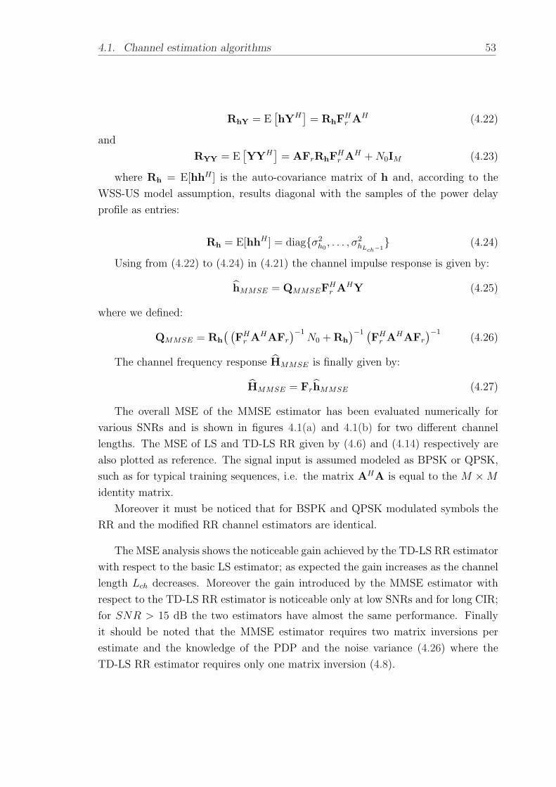
4.1. Channel estimation algorithms 53
RhY = E[hYH
]= RhF
Hr AH (4.22)
and
RYY = E[YYH
]= AFrRhF
Hr AH + N0IM (4.23)
where Rh = E[hhH ] is the auto-covariance matrix of h and, according to the
WSS-US model assumption, results diagonal with the samples of the power delay
profile as entries:
Rh = E[hhH ] = diagσ2h0
, . . . , σ2hLch−1
(4.24)
Using from (4.22) to (4.24) in (4.21) the channel impulse response is given by:
hMMSE = QMMSEFHr AHY (4.25)
where we defined:
QMMSE = Rh
( (FH
r AHAFr
)−1N0 + Rh
)−1 (FH
r AHAFr
)−1(4.26)
The channel frequency response HMMSE is finally given by:
HMMSE = FrhMMSE (4.27)
The overall MSE of the MMSE estimator has been evaluated numerically for
various SNRs and is shown in figures 4.1(a) and 4.1(b) for two different channel
lengths. The MSE of LS and TD-LS RR given by (4.6) and (4.14) respectively are
also plotted as reference. The signal input is assumed modeled as BPSK or QPSK,
such as for typical training sequences, i.e. the matrix AHA is equal to the M ×M
identity matrix.
Moreover it must be noticed that for BSPK and QPSK modulated symbols the
RR and the modified RR channel estimators are identical.
The MSE analysis shows the noticeable gain achieved by the TD-LS RR estimator
with respect to the basic LS estimator; as expected the gain increases as the channel
length Lch decreases. Moreover the gain introduced by the MMSE estimator with
respect to the TD-LS RR estimator is noticeable only at low SNRs and for long CIR;
for SNR > 15 dB the two estimators have almost the same performance. Finally
it should be noted that the MMSE estimator requires two matrix inversions per
estimate and the knowledge of the PDP and the noise variance (4.26) where the
TD-LS RR estimator requires only one matrix inversion (4.8).
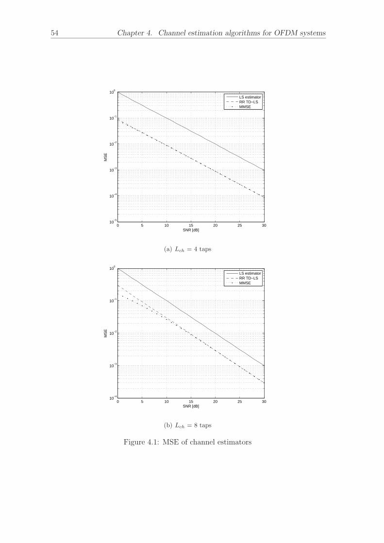
54 Chapter 4. Channel estimation algorithms for OFDM systems
0 5 10 15 20 25 3010
−5
10−4
10−3
10−2
10−1
100
SNR [dB]
MS
E
LS estimatorRR TD−LSMMSE
(a) Lch = 4 taps
0 5 10 15 20 25 3010
−4
10−3
10−2
10−1
100
SNR [dB]
MS
E
LS estimatorRR TD−LSMMSE
(b) Lch = 8 taps
Figure 4.1: MSE of channel estimators

4.2. Channel length estimation 55
4.2 Channel length estimation
The TD-LS RR channel estimator, the modified TD-LS channel estimator and the
MMSE channel estimator described in section 4.1 assumed the knowledge of the CIR
length Lch. The CIR length must be estimated in real systems; in the following a
channel length estimation algorithm is described.
In [12] it is proposed a joint estimation of the symbol timing, channel length and
channel impulse response for OFDM-based systems. In particular, an estimation al-
gorithm based on a reduced-rank approach and on a generalized Akaike information
criterion is presented. Under the assumption of correct symbol timing synchroniza-
tion, the algorithm proposed in [12] can efficiently be used to achieve a joint estima-
tion of Lch and of its CIR. Let P be the M × 1 vector containing the known data
samples of the LTS, as previously described in (3.2), and let YP = [yP,0; . . . ; yP,M−1]T
be the corresponding received signal.
Therefore, the proposed algorithm decreases the supposed length of the channel
impulse response from Ltest = Lcp until the following generalized Akaike information
criterion (GAIC) is minimized:
Lch = minLtest
(‖ lnFLtestYP − diag(P)FLtesth(Ltest)‖2 + γLtest
)(4.28)
where γ is a fixed constant [12], FLtest is the M ×Ltest RR DFT matrix described in
(4.1), and h(Ltest) is the reduced-rank LS estimation of the channel given the sup-
posed channel length Ltest, i.e., h(Ltest) = F+Ltest
YP , where h(Ltest) has dimensions
Ltest × 1.
In particular, from numerical simulations we found that a convenient value for γ
in (4.28) is γ = 0.03. The algorithm implements the following successive steps.
1. Fix Ltest = 16.
2. Compute the reduced-rank LS estimation of the channel given the supposed
channel length Ltest.
3. Compute (4.28).
4. Decrease Ltest and repeat points 2 ,3, 4, until (4.28) is minimized.
5. The value of Ltest = Lch that minimizes (4.28) gives the estimated channel
impulse response length, while the corresponding h(Lch) represents the esti-
mation of the channel impulse response that is used to initialize the channel
tracking algorithm.

56 Chapter 4. Channel estimation algorithms for OFDM systems
If the channel is assumed to be static over the whole LTS (which is a reasonable
assumption in the case under investigation) then the algorithm can use both symbols
in the LTS. Consequently, it can be modified as follows:
1. Fix Ltest = 16.
2. Compute the rr-LS estimation of the channel given the supposed channel length
Ltest over the first and second symbols of the LTS, obtaining h1(Ltest) and
h2(Ltest), respectively.
3. Set h(Ltest) = (h1(Ltest) + h2(Ltest))/2.
4. Compute (4.28).
5. Decrease Ltest and repeat point 2,3,4, until (4.28) is minimized.
6. The value of Ltest = Lch that minimizes (4.28) represents the channel impulse
response length, and the corresponding h(Lch) the estimated channel impulse
response.

Chapter 5
Decision directed channel
estimation for mobile OFDM
systems
5.1 Introduction
The wireless channel in vehicular environment is time variant, as also described in
detail in chapter 1. In section 5.1.1 the invariance time of the wireless channel will
be evaluated for a maximum relative speed of v = 260 km/h that is Tinv = Tcoh/10 =
1/(fD10) = 70.175 µs. This implies that within a single OFDM symbol the channel
can be considered static in simulations while from packet to the packet transmission
it has a time-varying behavior.1 In other words it is necessary to update the channel
estimate in order to correctly perform the equalization task.
The channel tracking task can be performed in various ways widely investigated
in literature; these techniques can be grouped into two categories:
• Pilot Assisted Channel Tracking (PACT) algorithms;
• Decision Directed Channel Estimation (DD-CE) algorithms.
1As an example a 2000 bytes PSDU 16-QAM modulated with code rate 1/2 generates a packetof 167 OFDM symbols, corresponding to a transmission time of 1336 µs.
57

58 Chapter 5. Decision directed channel estimation for mobile OFDM systems
5.1.1 Vehicular channel time invariance assessments
This section describes the time-varying effects introduced by the motion of the trans-
mitter and the receiver in vehicular environment, which motivate the necessity to
update the channel estimate in order to correctly perform the equalization task.
A maximum relative speed v in the order of 260 km/h is considered for V2V
communications to perform a preliminary assessment. The maximum Doppler shift
is:
fD =vfc,max
c= 1425 Hz (5.1)
where the maximum carrier frequency allowed in [3] is fc,max = 5.92 GHz (sec. 3.2).
According to the definition of the coherence time of the channel [1], the trans-
mission link can be considered almost time invariant for Tinv = Tcoh/10 = 1/10fD =
70.175 µs. In IEEE 802.11p specifications the OFDM symbol time T is T = 8 µs
(see table 3.3) so the channel can be considered invariant within a single OFDM
symbol.
The temporal distribution of the rays that determine the multipath nature of the
wireless channel can be usually considered constant for NS symbols if
∆τl = (v/c)NST (5.2)
that is the variation of the delays τl (1.15) for NST seconds, is negligible compared
to the temporal resolution Tc = 1/B of the system. It results that, considering a
radial movement between a transmitter and a receiver with relative velocity v, the
condition ∆τl ¿ Tc implies that
NS ¿ c
v
1
M + Lcp
(5.3)
where M is the total number of sub-carriers of the system, and Lcp is the length of
the cyclic prefix. By replacing in (5.3) the system parameters summarized in (cap.
3, table 3.3) and v = 260 Km/h, it results that NS ¿ 51900 so the time delays can
be considered constant for about NS∼= 500 consecutive OFDM symbols. Such value
is larger than the typical number of OFDM symbols per packet.
A possible undesired consequence of the Doppler spread introduced by the time-
varying nature of the wireless channel is that the orthogonality between sub-carriers
may not be guaranteed thus arising ICI. For an OFDM signal in presence of Doppler
Spread, several bounds on the ICI degradation effect exist in literature; in particular

5.1. Introduction 59
a significant bound applied to the WSS-US channel model has been introduced in [8].
Such an upper bound is:σ2
ICI
σ2sTX
≤ 1
12(2πfDTs)
2, (5.4)
where σ2ICI indicates the variance of the Inter carrier Interference modeled as additive
Gaussian noise; σ2sTX represents the variance of the useful part of the received signal;
Ts = MTc is the duration of an OFDM symbol after the cyclic prefix removal. In
this case for B = 10 MHz the length of an OFDM symbol after the cyclic prefix
removal is Ts = 6.4 µs, and considering that for v = 260 Km/h it results fD = 1425
Hz, the upper bound (5.4) for the ICI power expressed in dB is
(σ2
ICI
σ2sTX
)
dB
= 10 log10
(1
12(2πfDT )2
)∼= −33.69dB. (5.5)
The ICI effect introduced by the Doppler spread values under consideration can
practically be neglected.
5.1.2 Channel tracking algorithms
Pilot Assisted Channel Tracking PACT techniques make use of the pilot sym-
bols inserted in the OFDM symbols together with data. The algorithm proposed
in [14] performs the task in two steps: first the CFR is evaluated on pilot sub-
carriers in the MMSE sense. Then the CFR is evaluated on the whole transmission
bandwidth by linear interpolation. The system considered is an OFDM system with
1024 sub-carriers and 128 pilot tones.
The main advantage of PACT techniques is the low complexity required by the es-
timator with reference to the DD-CE algorithms. The drawback is that in particular
conditions the pilot tones are insufficient to perform the CE accurately.
Decision Directed Channel Estimation Decision directed (DD), also known
as Data-Aided, CE algorithms make use of the received data to update the channel
estimation available at the receiver. DD techniques are used in two scenarios: first of
all if the considered system does not contain periodic sequences of pilot tones PACT
techniques are not suitable to perform the task. Moreover in [13] it has been shown
that in order to estimate the CIR (or equivalently the CFR) the number of pilots Np
must be equal to or higher than the CIR length Lch. The number of pilot tones per
OFDM symbol specified in [3] is Np = 4, that in many practical situations is smaller

60 Chapter 5. Decision directed channel estimation for mobile OFDM systems
than the channel length; a higher number of known symbols becomes necessary to
accurately perform the CE task.
The main idea behind DD-CE is the reconstruction of the transmitted OFDM
symbol in order to consider the received data as a training sequence and perform
CE exploiting the new available information. The main steps of a generic DD-CE
algorithm, given a received OFDM symbol Yk at time instant k, is the following:
1. equalization of the i−th sub-carrier of the received symbol Yk[i] with the avail-
able CFR Hk−1[i] as Xk[i] = Yk[i]/Hk−1[i];
2. hard or soft detection of the estimated symbol Ak to achieve the symbol se-
quence Ak. The hard detection implies hard demapping of the received symbol
by associating the closest QAM symbol Ak[i] (from the point of view of the
Euclidean distance from the received symbol) to the received equalized symbol
Xk[i]. Soft detection implies the decoding of the estimated symbol (eventu-
ally preceded by an appropriate deinterleaving operation) and the re-encoding,
interleaving and QAM mapping of the decoded bit sequence in order to recon-
struct the transmitted OFDM symbol after the error correction achieved by
the decoder.
3. estimation of Hk performed using as input the received symbol Yk and the
reconstructed Ak;
4. store the new channel estimate Hk for the following received symbol and use
it to perform the final equalization and decoding of the current k−th OFDM
symbol.
The two different approaches to DD-CE are shown in figures 5.1 and 5.2.
5.2 Decision directed channel estimation
In literature DD-CE has been widely explored because of the high performance
achievable. Under the assumption of perfect symbol duplication, the DD-CE be-
comes equivalent to CE performed with a known training sequence according to a
specific algorithm as reviewed in 4.1.
The main drawback of DD-CE is the presence of incorrect detected symbols in
the duplication loop that cause error propagation in the CE. The main focus in
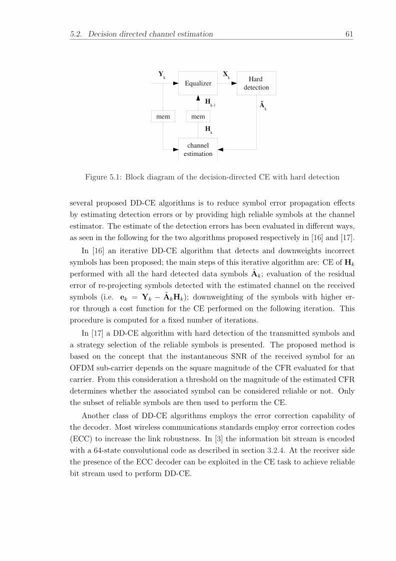
5.2. Decision directed channel estimation 61
Figure 5.1: Block diagram of the decision-directed CE with hard detection
several proposed DD-CE algorithms is to reduce symbol error propagation effects
by estimating detection errors or by providing high reliable symbols at the channel
estimator. The estimate of the detection errors has been evaluated in different ways,
as seen in the following for the two algorithms proposed respectively in [16] and [17].
In [16] an iterative DD-CE algorithm that detects and downweights incorrect
symbols has been proposed; the main steps of this iterative algorithm are: CE of Hk
performed with all the hard detected data symbols Ak; evaluation of the residual
error of re-projecting symbols detected with the estimated channel on the received
symbols (i.e. ek = Yk − AkHk); downweighting of the symbols with higher er-
ror through a cost function for the CE performed on the following iteration. This
procedure is computed for a fixed number of iterations.
In [17] a DD-CE algorithm with hard detection of the transmitted symbols and
a strategy selection of the reliable symbols is presented. The proposed method is
based on the concept that the instantaneous SNR of the received symbol for an
OFDM sub-carrier depends on the square magnitude of the CFR evaluated for that
carrier. From this consideration a threshold on the magnitude of the estimated CFR
determines whether the associated symbol can be considered reliable or not. Only
the subset of reliable symbols are then used to perform the CE.
Another class of DD-CE algorithms employs the error correction capability of
the decoder. Most wireless communications standards employ error correction codes
(ECC) to increase the link robustness. In [3] the information bit stream is encoded
with a 64-state convolutional code as described in section 3.2.4. At the receiver side
the presence of the ECC decoder can be exploited in the CE task to achieve reliable
bit stream used to perform DD-CE.
62 Chapter 5. Decision directed channel estimation for mobile OFDM systems
Figure 5.2: Block diagram of the data decoding-aided CE
With respect to the scheme represented in figure 5.1 that uses hard detected
symbols, the introduction of the decoder in the CE task (figure 5.2) requires the
hardware implementation of dedicated components such as the encoder and the in-
terleaver and higher computational requirements due to the more complex symbol
duplication loop.
According to this DD-CE scheme, Abdulhamid et al. in [18] introduce a forgetting
factor in order to provide the equalizer with a CIR weighted with the past estimates
CIRs (in the LS sense) and achieve a reduction in the estimation error. A similar
approach has been proposed in [19] where a forgetting factor weighs the present and
past channel estimates (in the MMSE sense) summed together to achieve the CIR
provided at the equalizer. Furthermore in [19] authors introduce a threshold on the
variation between CFR on adjacent sub-carriers in order to detect the temporarily
distorted sub-carriers: in other words the sub-channels that differ more than a specific
threshold with the adjacent carriers are considered momentarily distorted and the
value of the CFR estimated in that carrier is replaced with the value estimated in
the previous CE for the same carrier.
In [20] a DD-CE algorithm with Viterbi decoder and symbol duplication is pro-
posed that takes into account the intrinsic delay introduced by the Viterbi decoder to
provide reliable decoded bits. In more details in the proposed algorithm a delay of M
OFDM symbols has been introduced before obtaining the decoded bit stream as out-
put of the Viterbi decoder to guarantee the convergence of the decoded stream. This
delay introduced in the decoding block leads to a delay in the symbol duplication
loop and consequently in the estimated OFDM symbol, i.e. Xk[i] = Yk[i]/Hk−M [i].
In the following sections the convergence time and the reliability of the decoded

5.3. Data decoding aided channel estimation 63
bit sequence will be investigated. These considerations will justify the unnecessity
of the delay M > 1 OFDM symbol introduced in [20]; moreover a simplified DD-CE
scheme with FEC (with respect to the DD-CE schemes presented in [18] and [19])
will be presented, together with simulation results of PER vs. SNR.
5.3 Data decoding aided channel estimation
5.3.1 First scheme: iterative data decoding aided CE
The first DD-CE scheme studied and proposed in figure 5.3 is an iterative FEC
scheme that makes use of two Viterbi decoders. The first decodes the received symbol
Yk equalized with the CFR Hk−1 estimated with the previous received symbol. The
second decodes the received symbol Yk equalized with the updated channel estimate
Hk. After the channel estimator a second Viterbi decoder is used to decode the
received symbol equalized with the new channel estimated to obtain the final decoded
bit stream. The main steps are the following:
1. the received OFDM symbol Yk is first equalized with the channel estimate
Hk−1 determined at the (k − 1)−th time instant;
2. the estimated OFDM symbol Xk is the input of the block sequence composed
of soft demapper, deinterleaver and Viterbi decoder;
3. the decoded bit stream bk is re-encoded, interleaved and mapped to obtain the
duplicated transmitted OFDM symbol Ak;
4. the channel estimate update Hk is computed from the received symbol Yk and
the duplicated symbol Ak and stored in memory;
5. the received OFDM symbol Yk is equalized with the updated channel estimate
Hk to obtain the updated OFDM symbol estimate X′k;
6. the updated OFDM symbol estimate is demapped, deinterleaved and decoded
to achieve the final decoded bit sequence b′k of the k−th OFDM symbol;
7. the received OFDM symbol Yk+1 is equalized and a further loop iteration
begins.
Some observations on the described scheme are worth noticing :

64 Chapter 5. Decision directed channel estimation for mobile OFDM systems
Figure 5.3: Iterative data decoding-aided CE block diagram - scheme 1
Figure 5.4: Iterative data decoding-aided CE block diagram - scheme 2

5.3. Data decoding aided channel estimation 65
• the presented scheme has an OFDM symbol approach: every block works itera-
tively with a period corresponding to the OFDM symbol time. This is possible
because the interleaver [3] operates on blocks of encoded bits with length cor-
responding to the number of encoded bit per OFDM symbol for the specific
modulation rate (NCPSC , table 3.3), i.e. it introduces one OFDM symbol la-
tency.
• The constraint length of the 64-state convolutional encoder [3] is c = 6. It is
a common assumption to evaluate the convergence time of the bit sequence
out of the Viterbi decoder as tconv ∼ 4c = 24. In IEEE 802.11p transmission
schemes the convergence time of 24 decoded bits is always lower than one
OFDM symbol length: the worst case is the BPSK 1/2 modulation scheme
that implies the presence of 24 information bits per OFDM symbols.
• The proposed iterative scheme has high computational and latency require-
ments with respect to a DD-CE with no FEC scheme because of the additional
encoder and interleaver blocks, as well as the Viterbi decoder and deinterleaver.
The scheme illustrated in Figure 5.3 duplicates the sequence of soft demapper,
deinterleaver and Viterbi decoder blocks; in principle, they could operate in parallel
on two consecutive input OFDM symbols in order to minimize the time latency. In
this case the impact on chip area compared to a commercial off-the shelf (COTS)
802.11a/g receiver is significant as many important blocks are duplicated. In alterna-
tive, and this justifies the “iterative” character of the scheme, the same performance
can be obtained by iterating the data flow over a single Viterbi FEC instantiation,
which in such case should be clocked at double frequency in order to employ the
same processing time. An example is illustrated in figure 5.4.
5.3.2 Second scheme: non-iterative data decoding aided CE
A simplified non-iterative scheme has also been investigated. The main idea behind
the non-iterative data-decoding aided CE scheme is to make use of a single Viterbi
decoder and use the output bit stream at the same time for the CE task and as final
output information bit stream. The block diagram is shown in figure 5.5; the main
steps are the following:
1. the received OFDM symbol Yk is equalized with most recent available channel
estimate Hk−1;
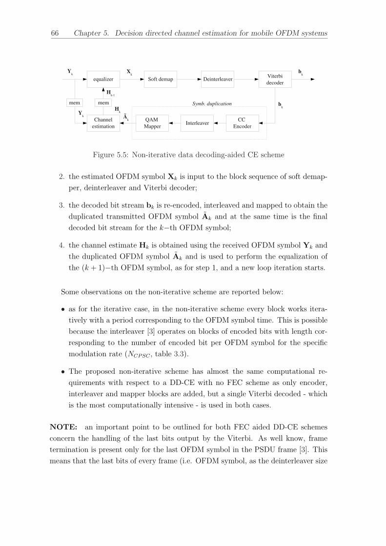
66 Chapter 5. Decision directed channel estimation for mobile OFDM systems
Figure 5.5: Non-iterative data decoding-aided CE scheme
2. the estimated OFDM symbol Xk is input to the block sequence of soft demap-
per, deinterleaver and Viterbi decoder;
3. the decoded bit stream bk is re-encoded, interleaved and mapped to obtain the
duplicated transmitted OFDM symbol Ak and at the same time is the final
decoded bit stream for the k−th OFDM symbol;
4. the channel estimate Hk is obtained using the received OFDM symbol Yk and
the duplicated OFDM symbol Ak and is used to perform the equalization of
the (k + 1)−th OFDM symbol, as for step 1, and a new loop iteration starts.
Some observations on the non-iterative scheme are reported below:
• as for the iterative case, in the non-iterative scheme every block works itera-
tively with a period corresponding to the OFDM symbol time. This is possible
because the interleaver [3] operates on blocks of encoded bits with length cor-
responding to the number of encoded bit per OFDM symbol for the specific
modulation rate (NCPSC , table 3.3).
• The proposed non-iterative scheme has almost the same computational re-
quirements with respect to a DD-CE with no FEC scheme as only encoder,
interleaver and mapper blocks are added, but a single Viterbi decoded - which
is the most computationally intensive - is used in both cases.
NOTE: an important point to be outlined for both FEC aided DD-CE schemes
concern the handling of the last bits output by the Viterbi. As well know, frame
termination is present only for the last OFDM symbol in the PSDU frame [3]. This
means that the last bits of every frame (i.e. OFDM symbol, as the deinterleaver size

5.3. Data decoding aided channel estimation 67
corresponds to the length of an OFDM symbol) input to the Viterbi will produce
non reliable decoder decisions unless a following OFDM symbol is appended to the
current one. This is considered tolerable for CE purposes; for the output bit stream
the last portion of the decoded frame has a delay of one OFDM symbol in order to
guarantee the reliability convergence.
The performance results shown in sec. 5.3.3 for both schemes correspond to:
• introduce one OFDM symbol delay latency in order to generate the decoded
information bits output by the Viterbi; in other words, the information bits
corresponding to the k-th OFDM symbol are decoded only after the (k+1)−th
symbol is processed too;
• however in both cases, the updated channel estimates need to be ready in time
to equalize the (k + 1)−th OFDM symbol: this is accomplished tolerating less
reliable bits in the last portion of the Viterbi output frame used for symbol
duplication and CE purposes.
5.3.3 Performance results
The simulation results for iterative and non-iterative schemes are presented in figures
5.6 to 5.50 in terms of packet error rate (PER) vs. SNR for ETSI B and ETSI C
channels and Jakes Doppler effect with various relative speeds. The values considered
of the simulation parameters are summarized in table 5.1.
Unless otherwise stated, the performance curves of PER vs. SNR presented in
this thesis are obtained as follows:
• for every simulated packet an independent channel realization is taken into
account;
• the Doppler effect is added to the channel realization and its temporal evolution
is observed for the whole packet transmission;
• the average per packet channel energy is normalized to the unitary value.
Performance curves obtained with perfect CIR knowledge and with DD-CE em-
ploying hard detection performed with all data and with SSA [17] are also plotted
as reference. With respect to the legend taken into account in the selected figures,
Perfect CIR employs the perfect knowledge of the CIR; TD-LS all data employs the

68 Chapter 5. Decision directed channel estimation for mobile OFDM systems
TD-LS RR CE (sec. 4.1.2), TD-LS SSA thr 0.05 employs the DD-CE algorithm
presented in [17], TD-LS iterative Vit. employs the scheme presented in sec. 5.3.1
and TD-LS iterative Vit. employs the scheme presented in sec. 5.3.2.
In every DD-CE scheme considered the employed CE is the TD-LS technique
exploiting the knowledge of the CIR length as described in sec. 4.1.2. Moreover
ideal time and frequency synchronization at the receiver has been considered.
Parameter Simulated values
Bandwidth 10 MHz
Data rates 6, 12, 27 Mbps
Packet length L 50, 400, 2000 bytes
Channel models ETSI B, C
Relative speed v 60, 120, 200 km/h
CIR length estimated
Channel estimation TD-LS RR
Simulated frames per SNR value 3000
Table 5.1: Values of the simulated scenarios

5.3. Data decoding aided channel estimation 69
0 2 4 6 8 10 12 14 1610
−2
10−1
100
SNR [dB]
PE
R
Perfect CIRTD−LS all data802.11aTD−LS SSA thr 0.05TD−LS iterative VitTD−LS non−iterative Vit
Figure 5.6: PER vs. SNR. ETSI B, v = 60 km/h, QPSK 1/2, L = 50 B
0 2 4 6 8 10 12 14 16 18 2010
−2
10−1
100
SNR [dB]
PE
R
Perfect CIRTD−LS all dataTD−LS SSA thr 0.05TD−LS iterative VitTD−LS non−iterative Vit
Figure 5.7: PER vs. SNR. ETSI B, v = 60 km/h, QPSK 1/2, L = 400 B
0 2 4 6 8 10 12 14 16 18 20 22 24 26 28 3010
−2
10−1
100
SNR [dB]
PE
R
Perfect CIRTD−LS All dataTD−LS SSA thr 0.05TD−LS iterative VitTD−LS non−iterative Vit
Figure 5.8: PER vs. SNR. ETSI B, v = 60 km/h, QPSK 1/2, L = 2000 B

70 Chapter 5. Decision directed channel estimation for mobile OFDM systems
4 5 6 7 8 9 10 11 12 13 1410
−2
10−1
100
SNR [dB]
PE
R
Perfect CIRTD−LS all data802.11aTD−LS SSA thr 0.05TD−LS iterative VitTD−LS non−iterative Vit
Figure 5.9: PER vs. SNR. ETSI B, v = 60 km/h, 16-QAM 1/2, L = 50 B
4 6 8 10 12 14 16 18 2010
−2
10−1
100
SNR [dB]
PE
R
Perfect CIRTD−LS all dataTD−LS SSA thr 0.05TD−LS iterative VitTD−LS non−iterative Vit
Figure 5.10: PER vs. SNR. ETSI B, v = 60 km/h, 16-QAM 1/2, L = 400 B
6 8 10 12 14 16 18 20 22 24 26 28 3010
−2
10−1
100
SNR [dB]
PE
R
Perfect CIRTD−LS All dataTD−LS SSA thr 0.05TD−LS iterative VitTD−LS non−iterative Vit
Figure 5.11: PER vs. SNR. ETSI B, v = 60 km/h, 16-QAM 1/2, L = 2000 B

5.3. Data decoding aided channel estimation 71
14 15 16 17 18 19 20 21 22 23 24 25 2610
−2
10−1
100
SNR [dB]
PE
R
Perfect CIRTD−LS all data802.11aTD−LS SSA thr 0.05TD−LS iterative VitTD−LS non−iterative Vit
Figure 5.12: PER vs. SNR. ETSI B, v = 60 km/h, 64-QAM 3/4, L = 50 B
14 16 18 20 22 24 26 28 3010
−2
10−1
100
SNR [dB]
PE
R
Perfect CIRTD−LS all dataTD−LS SSA thr 0.05TD−LS iterative VitTD−LS non−iterative Vit
Figure 5.13: PER vs. SNR. ETSI B, v = 60 km/h, 64-QAM 3/4, L = 400 B
14 16 18 20 22 24 26 28 3010
−2
10−1
100
SNR [dB]
PE
R
Perfect CIRTD−LS All dataTD−LS SSA thr 0.05TD−LS iterative VitTD−LS non−iterative Vit
Figure 5.14: PER vs. SNR. ETSI B, v = 60 km/h, 64-QAM 3/4, L = 2000 B

72 Chapter 5. Decision directed channel estimation for mobile OFDM systems
0 2 4 6 8 10 12 14 16 18 2010
−2
10−1
100
SNR [dB]
PE
R
Perfect CIRTD−LS all data802.11aTD−LS SSA thr 0.05TD−LS iterative VitTD−LS non−iterative Vit
Figure 5.15: PER vs. SNR. ETSI B, v = 120 km/h, QPSK 1/2, L = 50 B
0 2 4 6 8 10 12 14 16 18 20 22 24 26 28 3010
−2
10−1
100
SNR [dB]
PE
R
Perfect CIRTD−LS all dataTD−LS SSA thr 0.05TD−LS iterative VitTD−LS non−iterative Vit
Figure 5.16: PER vs. SNR. ETSI B, v = 120 km/h, QPSK 1/2, L = 400 B
0 2 4 6 8 10 12 14 16 18 20 22 24 26 28 3010
−2
10−1
100
SNR [dB]
PE
R
Perfect CIRTD−LS All dataTD−LS SSA thr 0.05TD−LS iterative VitTD−LS non−iterative Vit
Figure 5.17: PER vs. SNR. ETSI B, v = 120 km/h, QPSK 1/2, L = 2000 B

5.3. Data decoding aided channel estimation 73
4 6 8 10 12 14 16 18 20 22 24 26 28 3010
−2
10−1
100
SNR [dB]
PE
R
Perfect CIRTD−LS all data802.11aTD−LS SSA thr 0.05TD−LS iterative VitTD−LS non−iterative Vit
Figure 5.18: PER vs. SNR. ETSI B, v = 120 km/h, 16-QAM 1/2, L = 50 B
6 8 10 12 14 16 18 20 22 24 26 28 3010
−2
10−1
100
SNR [dB]
PE
R
Perfect CIRTD−LS all dataTD−LS SSA thr 0.05TD−LS iterative VitTD−LS non−iterative Vit
Figure 5.19: PER vs. SNR. ETSI B, v = 120 km/h, 16-QAM 1/2, L = 400 B
8 10 12 14 16 18 20 22 24 26 28 3010
−2
10−1
100
SNR [dB]
PE
R
Perfect CIRTD−LS All dataTD−LS SSA thr 0.05TD−LS iterative VitTD−LS non−iterative Vit
Figure 5.20: PER vs. SNR. ETSI B, v = 120 km/h, 16-QAM 1/2, L = 2000 B

74 Chapter 5. Decision directed channel estimation for mobile OFDM systems
14 16 18 20 22 24 26 28 3010
−2
10−1
100
SNR [dB]
PE
R
Perfect CIRTD−LS all data802.11aTD−LS SSA thr 0.05TD−LS iterative VitTD−LS non−iterative Vit
Figure 5.21: PER vs. SNR. ETSI B, v = 120 km/h, 64-QAM 3/4, L = 50 B
14 16 18 20 22 24 26 28 3010
−2
10−1
100
SNR [dB]
PE
R
Perfect CIRTD−LS all dataTD−LS SSA thr 0.05TD−LS iterative VitTD−LS non−iterative Vit
Figure 5.22: PER vs. SNR. ETSI B, v = 120 km/h, 64-QAM 3/4, L = 400 B
16 18 20 22 24 26 28 3010
−2
10−1
100
SNR [dB]
PE
R
Perfect CIR
TD−LS All data
TD−LS SSA thr 0.05
TD−LS iterative Vit
TD−LS non−iterative Vit
Figure 5.23: PER vs. SNR. ETSI B, v = 120 km/h, 64-QAM 3/4, L = 2000 B
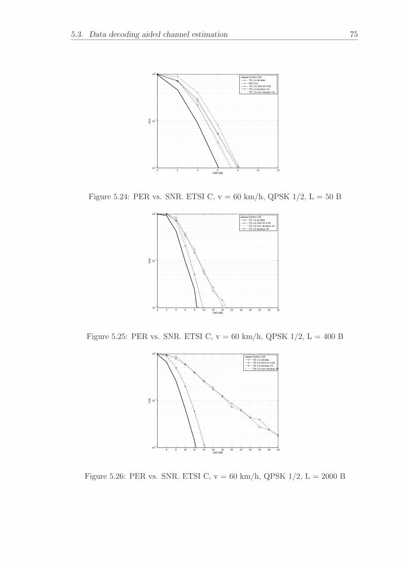
5.3. Data decoding aided channel estimation 75
0 2 4 6 8 10 1210
−2
10−1
100
SNR [dB]
PE
R
Perfect CIRTD−LS all data802.11aTD−LS SSA thr 0.05TD−LS iterative VitTD−LS non−iterative Vit
Figure 5.24: PER vs. SNR. ETSI C, v = 60 km/h, QPSK 1/2, L = 50 B
0 2 4 6 8 10 12 14 16 18 20 22 24 2610
−2
10−1
100
SNR [dB]
PE
R
Perfect CIRTD−LS all dataTD−LS SSA thr 0.05TD−LS non−iterative VitTD−LS iterative Vit
Figure 5.25: PER vs. SNR. ETSI C, v = 60 km/h, QPSK 1/2, L = 400 B
6 8 10 12 14 16 18 20 22 24 26 28 3010
−2
10−1
100
SNR [dB]
PE
R
Perfect CIRTD−LS all dataTD−LS SSA thr 0.05TD−LS iterative VitTD−LS non−iterative Vit
Figure 5.26: PER vs. SNR. ETSI C, v = 60 km/h, QPSK 1/2, L = 2000 B

76 Chapter 5. Decision directed channel estimation for mobile OFDM systems
4 5 6 7 8 9 10 11 12 13 14 15 1610
−2
10−1
100
SNR [dB]
PE
R
Perfect CIRTD−LS all data802.11aTD−LS SSA thr 0.05TD−LS iterative VitTD−LS all non−iterative Vit
Figure 5.27: PER vs. SNR. ETSI C, v = 60 km/h, 16-QAM 1/2, L = 50 B
6 8 10 12 14 16 18 20 22 24 26 28 3010
−2
10−1
100
SNR [dB]
PE
R
Perfect CIRTD−LS all dataTD−LS SSA thr 0.05TD−LS iterative VitTD−LS non−iterative Vit
Figure 5.28: PER vs. SNR. ETSI C, v = 60 km/h, 16-QAM 1/2, L = 400 B
8 10 12 14 16 18 20 22 24 26 28 3010
−2
10−1
100
SNR [dB]
PE
R
Perfect CIRTD−LS all dataTD−LS SSA thr 0.05TD−LS iterative VitTD−LS non−iterative Vit
Figure 5.29: PER vs. SNR. ETSI C, v = 60 km/h, 16-QAM 1/2, L = 2000 B

5.3. Data decoding aided channel estimation 77
14 15 16 17 18 19 20 21 22 23 24 25 26 27 28 29 3010
−2
10−1
100
SNR [dB]
PE
R
Perfect CIRTD−LS all data802.11aTD−LS SSA thr 0.05TD−LS iterative VitTD−LS non−iterative Vit
Figure 5.30: PER vs. SNR. ETSI C, v = 60 km/h, 64-QAM 3/4, L = 50 B
14 16 18 20 22 24 26 28 3010
−2
10−1
100
SNR [dB]
PE
R
Perfect CIRTD−LS all dataTD−LS SSA thr 0.05TD−LS iterative VitTD−LS non−iterative Vit
Figure 5.31: PER vs. SNR. ETSI C, v = 60 km/h, 64-QAM 3/4, L = 400 B
14 16 18 20 22 24 26 28 3010
−2
10−1
100
SNR [dB]
PE
R
Perfect CIR
TD−LS all data
TD−LS SSA thr 0.05
TD−LS iterative Vit
TD−LS non−iterative Vit
Figure 5.32: PER vs. SNR. ETSI C, v = 60 km/h, 64-QAM 3/4, L = 2000 B

78 Chapter 5. Decision directed channel estimation for mobile OFDM systems
0 2 4 6 8 10 12 1410
−2
10−1
100
SNR
PE
R
Perfect CIRTD−LS all dataTD−LS SSA thr 0.05802.11aTD−LS iterative VitTD−LS non−iterative Vit
Figure 5.33: PER vs. SNR. ETSI C, v = 120 km/h, QPSK 1/2, L = 50 B
0 2 4 6 8 10 12 14 16 18 20 22 24 26 28 3010
−2
10−1
100
SNR
PE
R
Perfect CIRTD−LS all dataTD−LS SSA thr 0.05802.11aTD−LS iterative VitTD−LS non−iterative Vit
Figure 5.34: PER vs. SNR. ETSI C, v = 120 km/h, QPSK 1/2, L = 400 B
0 2 4 6 8 10 12 14 16 18 20 22 24 26 28 3010
−2
10−1
100
SNR
PE
R
Perfect CIRTD−LS all dataTD−LS SSA thr 0.05TD−LS iterative VitTD−LS non−iterative Vit
Figure 5.35: PER vs. SNR. ETSI C, v = 120 km/h, QPSK 1/2, L = 2000 B

5.3. Data decoding aided channel estimation 79
4 5 6 7 8 9 10 11 12 13 14 15 16 17 1810
−2
10−1
100
SNR
PE
R
Perfect CIRTD−LS all dataTD−LS SSA thr 0.05802.11aTD−LS iterative VitTD−LS non−iterative Vit
Figure 5.36: PER vs. SNR. ETSI C, v = 120 km/h, 16-QAM 1/2, L = 50 B
6 8 10 12 14 16 18 20 22 24 26 28 3010
−2
10−1
100
SNR
PE
R
Perfect CIRTD−LS all dataTD−LS SSA thr 0.05TD−LS iterative VitTD−LS non−iterative Vit
Figure 5.37: PER vs. SNR. ETSI C, v = 120 km/h, 16-QAM 1/2, L = 400 B
10 12 14 16 18 20 22 24 26 28 3010
−2
10−1
100
SNR
PE
R
Perfect CIR
TD−LS all data
TD−LS SSA thr 0.05
TD−LS iterative Vit
TD−LS non−iterative Vit
Figure 5.38: PER vs. SNR. ETSI C, v = 120 km/h, 16-QAM 1/2, L = 2000 B

80 Chapter 5. Decision directed channel estimation for mobile OFDM systems
14 16 18 20 22 24 26 28 3010
−2
10−1
100
SNR
PE
R
Perfect CIRTD−LS all dataTD−LS SSA thr 0.05802.11aTD−LS iterative VitTD−LS non−iterative Vit
Figure 5.39: PER vs. SNR. ETSI C, v = 120 km/h, 64-QAM 3/4, L = 50 B
14 16 18 20 22 24 26 28 3010
−2
10−1
100
SNR
PE
R
Perfect CIRTD−LS all dataTD−LS SSA thr 0.05TD−LS iterative VitTD−LS non−iterative Vit
Figure 5.40: PER vs. SNR. ETSI C, v = 120 km/h, 64-QAM 3/4, L = 400 B
16 18 20 22 24 26 28 3010
−2
10−1
100
SNR
PE
R
Perfect CIR
TD−LS All data
TD−LS SSA thr 0.05
TD−LS iterative Vit
TD−LS non−iterative Vit
Figure 5.41: PER vs. SNR. ETSI C, v = 120 km/h, 64-QAM 3/4, L = 2000 B

5.3. Data decoding aided channel estimation 81
0 1 2 3 4 5 6 7 8 9 10 11 1210
−2
10−1
100
SNR [dB]
PE
R
Perfect CIRTD−LS all data802.11aTD−LS SSA thr 0.05TD−LS iterative VitTD−LS non−iterative Vit
Figure 5.42: PER vs. SNR. ETSI C, v = 200 km/h, QPSK 1/2, L = 50 B
0 2 4 6 8 10 12 14 16 18 20 22 24 26 28 3010
−2
10−1
100
SNR [dB]
PE
R
Perfect CIRTD−LS all dataTD−LS SSA thr 0.05TD−LS iterative VitTD−LS non−iterative Vit
Figure 5.43: PER vs. SNR. ETSI C, v = 200 km/h, QPSK 1/2, L = 400 B
4 6 8 10 12 14 16 18 20 22 24 26 28 3010
−2
10−1
100
SNR [dB]
PE
R
Perfect CIR
TD−LS all data
TD−LS SSA thr 0.05
TD−LS iterative Vit
TD−LS non−iterative Vit
Figure 5.44: PER vs. SNR. ETSI C, v = 200 km/h, QPSK 1/2, L = 2000 B

82 Chapter 5. Decision directed channel estimation for mobile OFDM systems
4 5 6 7 8 9 10 11 12 13 14 15 16 17 1810
−2
10−1
100
SNR [dB]
PE
R
Perfect CIRTD−LS all data802.11aTD−LS SSA thr 0.05TD−LS iterative VitTD−LS non−iterative Vit
Figure 5.45: PER vs. SNR. ETSI C, v = 200 km/h, 16-QAM 1/2, L = 50 B
6 8 10 12 14 16 18 20 22 24 26 28 3010
−2
10−1
100
SNR [dB]
PE
R
Perfect CIRTD−LS All dataTD−LS SSA thr 0.05TD−LS iterative VitTD−LS non−iterative Vit
Figure 5.46: PER vs. SNR. ETSI C, v = 200 km/h, 16-QAM 1/2, L = 400 B
8 10 12 14 16 18 20 22 24 26 28 3010
−2
10−1
100
SNR [dB]
PE
R
Perfect CIR
TD−LS All data
TD−LS SSA thr 0.05
TD−LS iterative Vit
TD−LS non−iterative Vit
Figure 5.47: PER vs. SNR. ETSI C, v = 200 km/h, 16-QAM 1/2, L = 2000 B
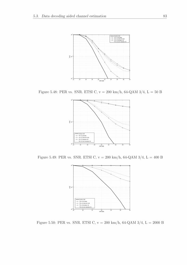
5.3. Data decoding aided channel estimation 83
12 14 16 18 20 22 24 26 28 3010
−2
10−1
100
SNR [dB]
PE
R
Perfect CIRTD−LS All dataTD−LS SSA thr 0.05TD−LS iterative VitTD−LS non−iterative Vit
Figure 5.48: PER vs. SNR. ETSI C, v = 200 km/h, 64-QAM 3/4, L = 50 B
14 16 18 20 22 24 26 28 3010
−2
10−1
100
SNR [dB]
PE
R
Perfect CIR
TD−LS all data
TD−LS SSA thr 0.05
TD−LS iterative Vit
TD−LS non−iterative Vit
Figure 5.49: PER vs. SNR. ETSI C, v = 200 km/h, 64-QAM 3/4, L = 400 B
18 20 22 24 26 28 3010
−2
10−1
100
SNR [dB]
PE
R
Perfect CIR
TD−LS All data
TD−LS SSA thr 0.05
TD−LS iterative Vit
TD−LS non−iterative Vit
Figure 5.50: PER vs. SNR. ETSI C, v = 200 km/h, 64-QAM 3/4, L = 2000 B

84 Chapter 5. Decision directed channel estimation for mobile OFDM systems
Rate [mbit/s] Modulationscheme
Coding rate Decoded bit perOFDM symbol
12 16-QAM 1/2 96
18 16-QAM 3/4 144
27 64-QAM 3/4 216
Table 5.2: Transmission parameters for Rates = 12, 18, 27 mbit/s
The simulation results show that forward error correction mitigates almost com-
pletely the error propagation effect. For both short (ETSI B) and long (ETSI C)
channels, data decoding aided DD-CE performs well even for high speed and high
modulation rates. A significant degradation of performance with reference to the
ideal case (i.e. perfect knowledge of CIR at the equalizer) is noticeable only in few
scenarios:
• Scenario 2: ETSI B 120 km/h - 64-QAM 3/4 L = 2000B;
• Scenario 5: ETSI C 200 km/h - 64-QAM 3/4 L = 400B;
• Scenario 5: ETSI C 200 km/h - 64-QAM 3/4 L = 2000B.
The two presented schemes of figures 5.3 and 5.5 have almost the same performance
in most scenarios, a degradation higher than 1 dB at PER = 0.1 can be seen only in
64-QAM 3/4 modulated packets.
To evaluate the impact on performance of the reliability of the decoded bits with
trellis truncation, the bit error probability (BER) as a function of the decoded bit
index within the frame is considered for rates 12, 18 and 27 Mbit/s under different
scenarios. The performance curves have been obtained simulating a total number of
200000 decoded OFDM symbols for every considered data rate.
These selected data rates permit to evaluate the BER in different modulation
schemes for the same coding rate (18 vs. 24 Mbit/s) or the BER in the same
modulation scheme for different coding rates (12 vs. 18 Mbit/s). In table 5.2 the
transmission parameters are summarized for the simulated rates.
Figures 5.51(a), 5.51(b) and 5.51(c) show the bit error probability (BER) out of
the Viterbi decoder for various relative speeds. As expected the last decoded bits of
the OFDM symbol result less reliable, in particular the assumed convergence time
tconv of 24 information bit for the 1/2 coding rate is confirmed by the performed
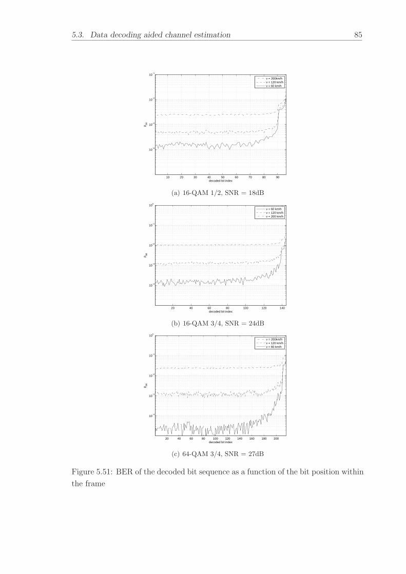
5.3. Data decoding aided channel estimation 85
10 20 30 40 50 60 70 80 90
10−4
10−3
10−2
10−1
decoded bit index
p bit
v = 200km/hv = 120 km/hv = 60 km/h
(a) 16-QAM 1/2, SNR = 18dB
20 40 60 80 100 120 140
10−4
10−3
10−2
10−1
100
decoded bit index
p bit
v = 60 km/hv = 120 km/hv = 200 km/h
(b) 16-QAM 3/4, SNR = 24dB
20 40 60 80 100 120 140 160 180 200
10−4
10−3
10−2
10−1
100
p bit
decoded bit index
v = 200km/hv = 120 km/hv = 60 km/h
(c) 64-QAM 3/4, SNR = 27dB
Figure 5.51: BER of the decoded bit sequence as a function of the bit position within
the frame
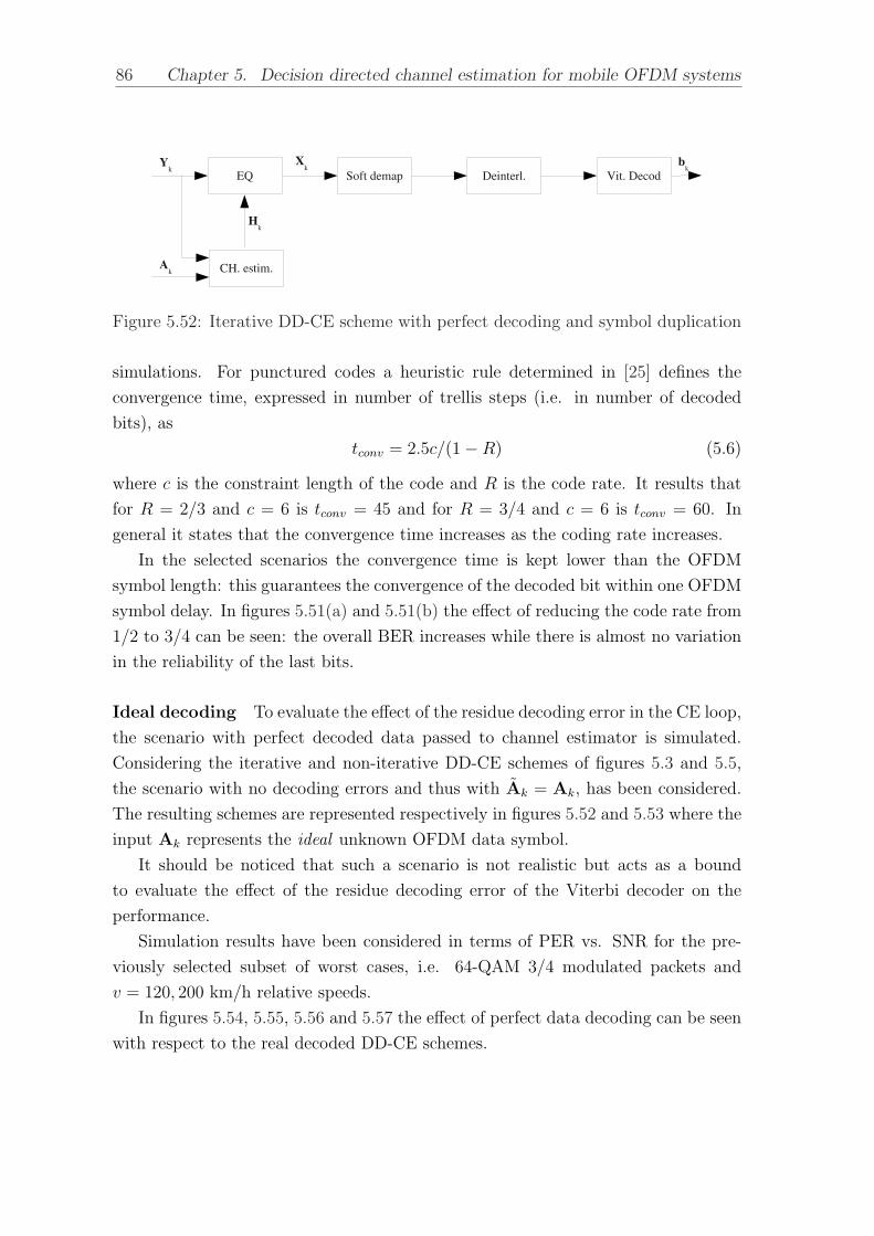
86 Chapter 5. Decision directed channel estimation for mobile OFDM systems
Figure 5.52: Iterative DD-CE scheme with perfect decoding and symbol duplication
simulations. For punctured codes a heuristic rule determined in [25] defines the
convergence time, expressed in number of trellis steps (i.e. in number of decoded
bits), as
tconv = 2.5c/(1−R) (5.6)
where c is the constraint length of the code and R is the code rate. It results that
for R = 2/3 and c = 6 is tconv = 45 and for R = 3/4 and c = 6 is tconv = 60. In
general it states that the convergence time increases as the coding rate increases.
In the selected scenarios the convergence time is kept lower than the OFDM
symbol length: this guarantees the convergence of the decoded bit within one OFDM
symbol delay. In figures 5.51(a) and 5.51(b) the effect of reducing the code rate from
1/2 to 3/4 can be seen: the overall BER increases while there is almost no variation
in the reliability of the last bits.
Ideal decoding To evaluate the effect of the residue decoding error in the CE loop,
the scenario with perfect decoded data passed to channel estimator is simulated.
Considering the iterative and non-iterative DD-CE schemes of figures 5.3 and 5.5,
the scenario with no decoding errors and thus with Ak = Ak, has been considered.
The resulting schemes are represented respectively in figures 5.52 and 5.53 where the
input Ak represents the ideal unknown OFDM data symbol.
It should be noticed that such a scenario is not realistic but acts as a bound
to evaluate the effect of the residue decoding error of the Viterbi decoder on the
performance.
Simulation results have been considered in terms of PER vs. SNR for the pre-
viously selected subset of worst cases, i.e. 64-QAM 3/4 modulated packets and
v = 120, 200 km/h relative speeds.
In figures 5.54, 5.55, 5.56 and 5.57 the effect of perfect data decoding can be seen
with respect to the real decoded DD-CE schemes.
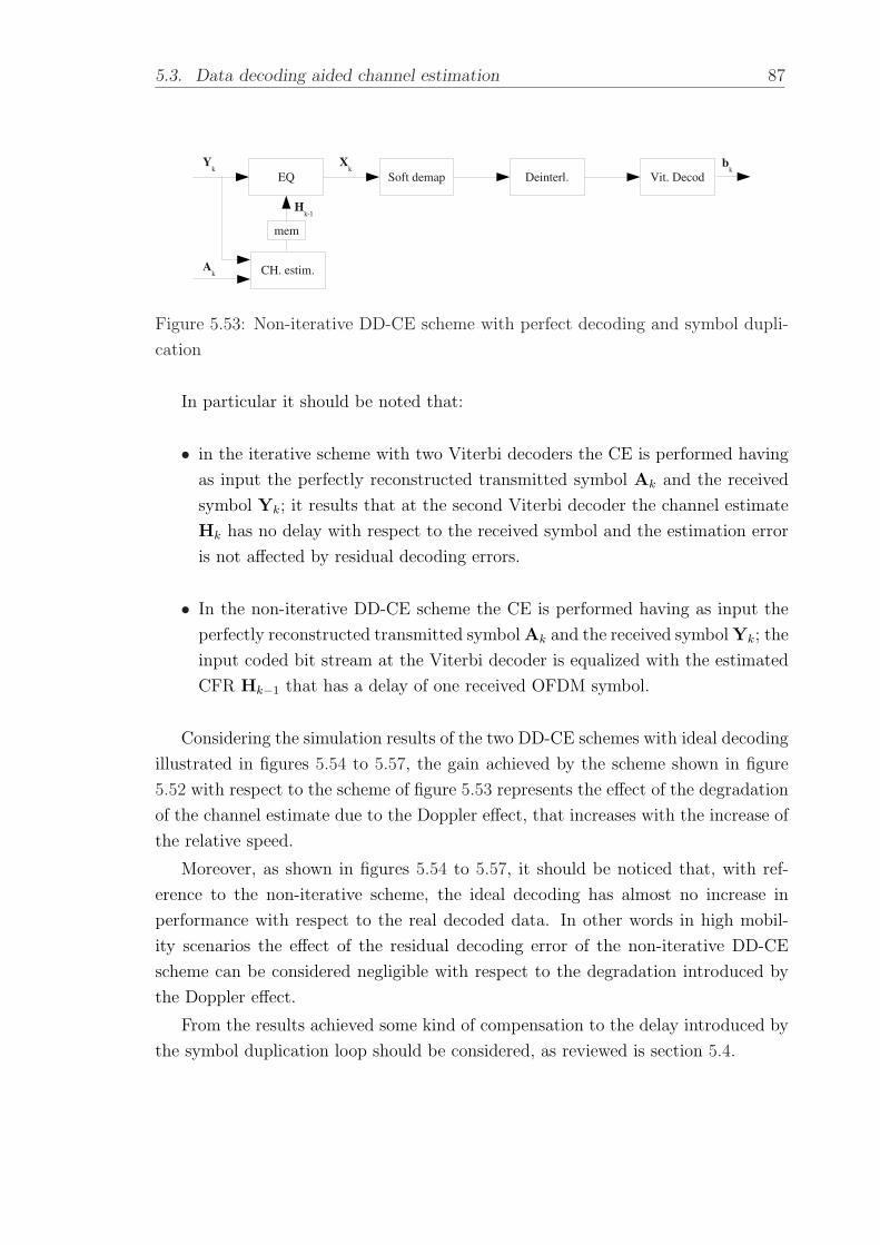
5.3. Data decoding aided channel estimation 87
Figure 5.53: Non-iterative DD-CE scheme with perfect decoding and symbol dupli-
cation
In particular it should be noted that:
• in the iterative scheme with two Viterbi decoders the CE is performed having
as input the perfectly reconstructed transmitted symbol Ak and the received
symbol Yk; it results that at the second Viterbi decoder the channel estimate
Hk has no delay with respect to the received symbol and the estimation error
is not affected by residual decoding errors.
• In the non-iterative DD-CE scheme the CE is performed having as input the
perfectly reconstructed transmitted symbol Ak and the received symbol Yk; the
input coded bit stream at the Viterbi decoder is equalized with the estimated
CFR Hk−1 that has a delay of one received OFDM symbol.
Considering the simulation results of the two DD-CE schemes with ideal decoding
illustrated in figures 5.54 to 5.57, the gain achieved by the scheme shown in figure
5.52 with respect to the scheme of figure 5.53 represents the effect of the degradation
of the channel estimate due to the Doppler effect, that increases with the increase of
the relative speed.
Moreover, as shown in figures 5.54 to 5.57, it should be noticed that, with ref-
erence to the non-iterative scheme, the ideal decoding has almost no increase in
performance with respect to the real decoded data. In other words in high mobil-
ity scenarios the effect of the residual decoding error of the non-iterative DD-CE
scheme can be considered negligible with respect to the degradation introduced by
the Doppler effect.
From the results achieved some kind of compensation to the delay introduced by
the symbol duplication loop should be considered, as reviewed is section 5.4.

88 Chapter 5. Decision directed channel estimation for mobile OFDM systems
16 18 20 22 24 26 28 3010
−2
10−1
100
SNR [dB]
PE
R
Perfect CIR
TD−LS iter.
TD−LS non−iter.
TD−LS non−iter. − bound
TD−LS iter. − bound
Figure 5.54: Ideal decoding - PER vs. SNR, v = 120 km/h, 64QAM 3/4, L = 2000
B
14 16 18 20 22 24 26 28 3010
−2
10−1
100
SNR [dB]
PE
R
Perfect CIR
TD−LS iter.
TD−LS non−iter.
TD−LS non−iter. − bound
TD−LS iter. − bound
Figure 5.55: Ideal decoding - PER vs. SNR, v = 200 km/h, 64QAM 3/4, L = 400 B

5.3. Data decoding aided channel estimation 89
18 20 22 24 26 28 3010
−2
10−1
100
SNR [dB]
PE
R
Perfect CIR
TD−LS iter.
TD−LS non−iter.
TD−LS non−iter. − bound
TD−LS iter. − bound
Figure 5.56: Ideal decoding - PER vs. SNR, v = 200 km/h, 64QAM 3/4, L = 2000
B
6 8 10 12 14 16 18 20 22 24 2610
−2
10−1
100
SNR [dB]
PE
R
Perfect CIRTD−LS iter.TD−LS non−iter.TD−LS non−iter. − boundTD−LS iter. − bound
Figure 5.57: Ideal decoding - PER vs. SNR, v = 200 km/h, 16QAM 1/2, L = 400 B
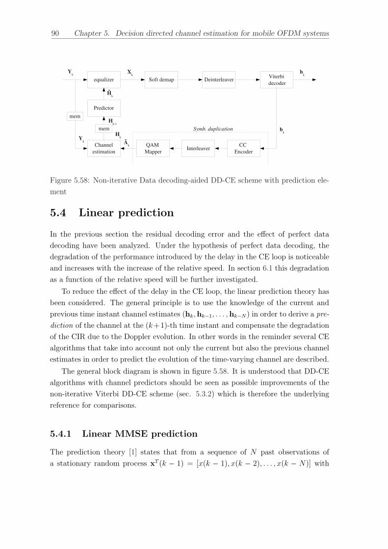
90 Chapter 5. Decision directed channel estimation for mobile OFDM systems
Figure 5.58: Non-iterative Data decoding-aided DD-CE scheme with prediction ele-
ment
5.4 Linear prediction
In the previous section the residual decoding error and the effect of perfect data
decoding have been analyzed. Under the hypothesis of perfect data decoding, the
degradation of the performance introduced by the delay in the CE loop is noticeable
and increases with the increase of the relative speed. In section 6.1 this degradation
as a function of the relative speed will be further investigated.
To reduce the effect of the delay in the CE loop, the linear prediction theory has
been considered. The general principle is to use the knowledge of the current and
previous time instant channel estimates (hk,hk−1, . . . ,hk−N) in order to derive a pre-
diction of the channel at the (k+1)-th time instant and compensate the degradation
of the CIR due to the Doppler evolution. In other words in the reminder several CE
algorithms that take into account not only the current but also the previous channel
estimates in order to predict the evolution of the time-varying channel are described.
The general block diagram is shown in figure 5.58. It is understood that DD-CE
algorithms with channel predictors should be seen as possible improvements of the
non-iterative Viterbi DD-CE scheme (sec. 5.3.2) which is therefore the underlying
reference for comparisons.
5.4.1 Linear MMSE prediction
The prediction theory [1] states that from a sequence of N past observations of
a stationary random process xT (k − 1) = [x(k − 1), x(k − 2), . . . , x(k − N)] with

5.4. Linear prediction 91
autocorrelation vector rTN = [rx(1), . . . , rx(N)], where the j−th entry is defined as
rx(j) = E[x(k)x∗(k − j)], the MMSE future estimation of x(k) is
x (k|x(k − 1)) =N∑
i=1
cix(k − i) (5.7)
that minimizes the prediction error:
fN(k) = x(k)− x (k|x(k − 1)) = x(k)−N∑
i=1
cix(k − i). (5.8)
The MSE of the predictor is J = E[|fN(k)|2]. The derivation of the optimum
coefficients cTopt = [copt,1, . . . , copt,N ] comes with the Wiener optimization theory [1].
It results that the optimum coefficient vector satisfies the equation:
RNcopt = rN (5.9)
where RN is the [N × N ] autocorrelation matrix of the process defined as RN =
E[x(k)xH(k)]. The minimum value of the cost function is
Jmin = JN = rx(0)− rHNcopt (5.10)
From equations (5.9) and (5.10) the following equation can be derived:[rx(0) rH
N
rN RN
][1
−copt
]=
[JN
0N
](5.11)
that can also be written as:
RN+1aTN =
[JN
0N
](5.12)
where 0N in the column vector of N zeros, RN+1 is the is the [N×N ] autocorrelation
matrix of the process with the (i, j)−th element defined as R(i,j) = E[x(k− j)x∗(k−i)], with i, j = 0, 1, . . . , N and
aTN = [1,−copt,1, . . . ,−copt,N ]. (5.13)
The optimum coefficient vector copt is obtained by solving the (5.12). The solution
of (5.12) can be efficiently computed with Levinson-Durbin algorithm [1].
As an example the vector aTN = [1,−copt,1,−copt,2] have been derived for the case
N = 2 past observations. It results that the optimum coefficients copt are:
copt,1 =rx(1)rx(0)− r∗x(1)rx(2)
r2x(0)− |rx(1)|2 (5.14)
92 Chapter 5. Decision directed channel estimation for mobile OFDM systems
and
copt,2 =rx(0)rx(2)− r2
x(1)
r2x(0)− |rx(1)|2 (5.15)
It must be noted that the formulation (5.9) recalls the Yule-Walker equation
defined as:
Ra = −r (5.16)
that gives the N × 1 coefficient vector a of the N−th order autoregressive (AR)
process with N × N autocorrelation matrix R and N × 1 autocorrelation vector
r. The AR model of a random process x(k) of order N with coefficient vector
a = [a1, a2, . . . , aN ] is defined as:
x(k) = −N∑
n=1
anx(k − n) + w(k) (5.17)
where w(k) is AWGN with variance σ2w.
In particular it results that the coefficients aTN = [1,−copt,1, . . . ,−copt,N ], solution
of (5.12), are the coefficients of the AR(N) model that approximate in the MMSE
sense the fading channel with autocorrelation matrix RN+1. In other words the co-
efficients aTN = [1,−copt,1, . . . ,−copt,N ] model both the MMSE predictor of a random
process x(k) given N past observations and the AR(N) model of the N -th order
autoregressive process that better approximates (in the MMSE sense) the process
x(k). These considerations will be taken into account in section 5.4.2.
The MMSE predictor can be applied to the CE algorithms. As shown in section
1.2.1, the wireless channel can be modeled as a WSS-US process with Tc spaced taps
defined as:
h(kT, nTc) =
Lch−1∑
l=0
hl(kT )δ(nTc − lTc) (5.18)
with Lch denoting the number of taps. It should be noted that the above equation
takes into account the US property of the hl(kT ) taps, l = 0, 1, . . . , Lch−1 and that,
in vehicular environment, the channel tap can be considered invariant within one
OFDM symbol period T for the typical relative speeds under consideration.
The related autocorrelation function is given by:
rh(∆t, ∆τ) = E[h(kT, τ)h∗(kT −∆t, τ −∆τ)
]=
Lch−1∑i=0
rhi(∆t)δ(∆τ − iTc) (5.19)

5.4. Linear prediction 93
and
rhl(∆t) = E
[hl(kT )h∗l (kT −∆t)
]. (5.20)
As said in section 5.1.1, a suitable Doppler spectrum for vehicular environment is the
classical Jakes model defined in (1.11) and applied independently to every channel
tap, for which (5.20) becomes:
rhl(∆t) = σ2
hlJ0(2πfD∆t) (5.21)
being fD the Doppler spread and J0(z) the first order Bessel function of first kind,
defined as:
J0(z) =∞∑
k=0
(−1)k
(z
2
)2k
(k!)2. (5.22)
The (i, j)-th element of the N ×N autocorrelation matrix Rhlof the l−th tap of
the fading channel with Jakes Doppler spectrum is Rhl,(i,j) = σ2hl
J0(2πfD(j − i)T ).
It results that the autocorrelation matrix Rhland the autocorrelation vector rhl
of
the l−th tap of the channel are the same for every tap, except for the multiplicative
factor σ2hl
. It results that the vector copt, solution of (5.9), is constant for every
channel tap.
As a first DD-CE scheme with predictor, MMSE linear prediction has been ap-
plied to the current and past estimated CIRs in order to provide a delay-free CIR to
the equalizer compared to the received OFDM symbol.
The l−th predicted channel tap hl(k + 1) at time instant (k + 1) is:
hl(k + 1) =k∑
i=1
copt,ihl(k − i). (5.23)
In vector notation the Lch × 1 predicted CIR hk+1 at time instant (k + 1) can be
written as:
hk+1 = hk,1copt (5.24)
where the Lch × k matrix hk,1 = [hk . . . ,h1]T has been defined as the matrix of the
k past estimated CIRs.
The coefficients copt applied independenlty to every tap are calculated from the
knowledge of the autocorrelation matrix Rhland the autocorrelation vector rhl
of
the l−th channel tap of the fading channel with Jakes spectrum. In particular, as
previously stated, the coefficients copt are independent from the factor σ2hl
that can
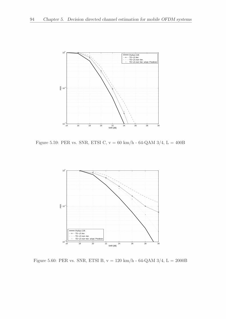
94 Chapter 5. Decision directed channel estimation for mobile OFDM systems
14 16 18 20 22 24 26 28 3010
−2
10−1
100
SNR [dB]
PE
R
Perfect CIRTD−LS iter.TD−LS non−iter.TD−LS non−iter. w/opt. Predictor
Figure 5.59: PER vs. SNR, ETSI C, v = 60 km/h - 64-QAM 3/4, L = 400B
16 18 20 22 24 26 28 3010
−2
10−1
100
SNR [dB]
PE
R
Perfect CIRTD−LS iter.TD−LS non−iter.TD−LS non−iter. w/opt. Predictor
Figure 5.60: PER vs. SNR, ETSI B, v = 120 km/h - 64-QAM 3/4, L = 2000B

5.4. Linear prediction 95
14 16 18 20 22 24 26 28 3010
−2
10−1
100
SNR [dB]
PE
R
Perfect CIRTD−LS iter.TD−LS non−iter.TD−LS non−iter. w/opt. Predictor
Figure 5.61: PER vs. SNR, ETSI C, v = 200 km/h - 64-QAM 3/4, L = 400B
18 20 22 24 26 28 3010
−2
10−1
100
SNR [dB]
PE
R
Perfect CIRTD−LS iter.TD−LS non−iter.TD−LS non−iter. w/opt. Predictor
Figure 5.62: PER vs. SNR, ETSI C, v = 200 km/h - 64-QAM 3/4, L = 2000B

96 Chapter 5. Decision directed channel estimation for mobile OFDM systems
be considered unitary; in other words the knowledge of the PDP σ2h1
, . . . , σ2hLch−1
of the channel is not necessary to derive copt.
Simulations of PER vs. SNR obtained using the scheme shown in figure 5.58 are
reported in figures 5.59, 5.60, 5.61 and 5.62 where the gain achieved by the MMSE
predictor can be observed. Further significant comments on the results are:
• in low-mobility scenarios the prediction element acts as an average of the CIRs
at various time instants; it results in a reduction of the CE error. In particular
in the case of no mobility, i.e. v = 0 km/h, the optimum coefficient vector
cTopt = [copt,1, . . . , copt,N ] is constant with elements copt,i = 1/N , i = 1, . . . , N ;
• in high mobility scenarios the prediction element compensates the degradation
introduced by the delay in the CE loop. In particular the highest improvement
can be seen for high data rate and high mobility.
Moreover it can be seen that MMSE prediction outperforms the iterative Viterbi
DD-CE scheme (sec. 5.3.1) without predictor where the final equalizer has no delay
between the channel estimate and the received OFDM symbol.
A possible motivation for this result is that, in the iterative scheme without
predictor, the degradation of the CIR due to the delay in the CE loop causes error
propagation that the Viterbi decoder is not able to recover.
The main drawbacks of this MMSE predictor are the high computational and
memory requirements (the actual memory size being related to the total number of
OFDM symbols per packet):
• all the past estimated CIRs for all the OFDM symbols in the packet must be
stored;
• the solution of the equation (5.12) must be updated for every received OFDM
symbol because of the always increasing number of input past CIRs and it
requires a number of operations proportional to k2, where k is the number of
past received OFDM symbols, when performed efficiently with the Levinson-
Durbin algorithm.
The computation of the optimum MMSE predictor is practically unfeasible in real
systems, but is is useful for simulations as an upper bound on performance gain
achievable by a prediction element.

5.4. Linear prediction 97
5.4.2 AR(N) model
The first simplification of the optimum MMSE predictor taken into account con-
siders a fixed number of N past estimated CIRs (corresponding to as many past
received OFDM symbols); it results that the optimum coefficient vector cTopt =
[copt,1, . . . , copt,N ] must be calculated only once (assuming the wireless chanel modeled
as a stationary process, otherwise the autocorrelation function is time-varying).
The method is computationally simpler because a fixed number of past input
CIRs translates into a limited predictor filter length and RN autocorrelation matrix
size. Such number can be chosen ad-hoc based on the desired trade-off between
performance and complexity.
The band-limited nature of the Doppler spectrum considered has consequently an
infinite-length autocorrelation function of the channel process. In [26] details on the
AR modeling for fading channels can be found; the authors derive the N×1 coefficient
vector a of the AR(N) process that better approximates the fading channel with Jakes
Doppler spectrum. As also previously reviewed in section 5.4.1 the coefficient vector
a of the AR(N) process is related to the relative optimum predictive coefficient vector
with the aTN = [1,−copt,1, . . . ,−copt,N ].
Moreover from the analysis presented in [26] the MSE σ2N = JN , defined in (5.4.1)
applied to the fading channel with Jakes Doppler spectrum, of the one-step AR(N)
predictor can be evaluated for a fixed filter length N as
σ2N ∼ k[sin(πfDT )]2N (5.25)
where k is a constant and T is the prediction time that equals to the OFDM symbol
time.
It should be noted that the normalized Doppler spread for a maximum relative
speed v = 260km/h is fDT = 1425T = 0.0114. In figure 5.63 the prediction error
σ2N of the AR(N) predictor as a function of the model order N is shown.
For the normalized maximum Doppler spread considered in vehicular scenarios
and for the frame structure of the IEEE 802.11p packet, the AR(2) approximation
of the fading channel with Jakes Doppler Spectrum has been chosen as trade-off:
as shown in section 3.2.3, in a IEEE 802.11p packet the OFDM data symbols are
preceded by a training sequence and the SIGNAL OFDM symbol modulated with
the most robust modulation (BPSK, code rate = 1/2).
Let “0” be the time instant of the first received data OFDM symbol, “-1” the
time instant of the received SIGNAL OFDM symbol and “-2” the time instant of
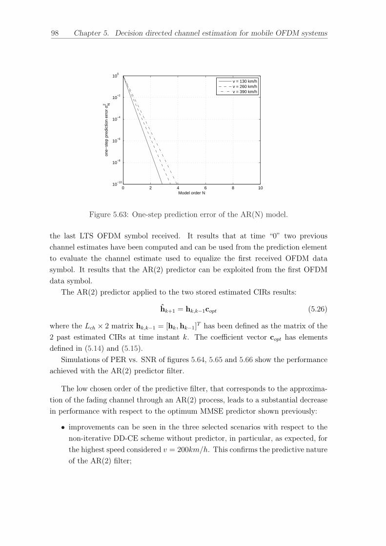
98 Chapter 5. Decision directed channel estimation for mobile OFDM systems
0 2 4 6 8 1010
−10
10−8
10−6
10−4
10−2
100
Model order N
one−
step
pre
dict
ion
erro
r σ2 N
v = 130 km/hv = 260 km/hv = 390 km/h
Figure 5.63: One-step prediction error of the AR(N) model.
the last LTS OFDM symbol received. It results that at time “0” two previous
channel estimates have been computed and can be used from the prediction element
to evaluate the channel estimate used to equalize the first received OFDM data
symbol. It results that the AR(2) predictor can be exploited from the first OFDM
data symbol.
The AR(2) predictor applied to the two stored estimated CIRs results:
hk+1 = hk,k−1copt (5.26)
where the Lch × 2 matrix hk,k−1 = [hk,hk−1]T has been defined as the matrix of the
2 past estimated CIRs at time instant k. The coefficient vector copt has elements
defined in (5.14) and (5.15).
Simulations of PER vs. SNR of figures 5.64, 5.65 and 5.66 show the performance
achieved with the AR(2) predictor filter.
The low chosen order of the predictive filter, that corresponds to the approxima-
tion of the fading channel through an AR(2) process, leads to a substantial decrease
in performance with respect to the optimum MMSE predictor shown previously:
• improvements can be seen in the three selected scenarios with respect to the
non-iterative DD-CE scheme without predictor, in particular, as expected, for
the highest speed considered v = 200km/h. This confirms the predictive nature
of the AR(2) filter;

5.4. Linear prediction 99
16 18 20 22 24 26 28 3010
−2
10−1
100
SNR [dB]
PE
R
Perfect CIRTD−LS iter.TD−LS non−iter.TD−LS non−iter. w/MMSE predictorTD−LS non−iter. w/AR(2) predictor
Figure 5.64: PER vs. SNR, DD-CE with AR(2) predictor - ETSI B, v = 120 km/h
- 64-QAM 3/4, L = 2000 B
14 16 18 20 22 24 26 28 3010
−2
10−1
100
SNR [dB]
PE
R
Perfect CIRTD−LS iter.TD−LS non−iter.TD−LS non−iter. w/MMSE predictorTD−LS non−iter. w/AR(2) predictor
Figure 5.65: PER vs. SNR, DD-CE with AR(2) predictor - ETSI C, v = 200 km/h
- 64-QAM 3/4, L = 400 B

100 Chapter 5. Decision directed channel estimation for mobile OFDM systems
18 20 22 24 26 28 3010
−2
10−1
100
SNR [dB]
PE
R
Perfect CIRTD−LS iter.TD−LS non−iter.TD−LS non−iter. w/MMSE predictorTD−LS non−iter. w/AR(2) predictor
Figure 5.66: PER vs. SNR, DD-CE with AR(2) predictor - ETSI C, v = 200 km/h
- 64-QAM 3/4, L = 2000 B
• the decrease in performance with respect to the MMSE predictor confirms the
sub-optimal nature of the AR(2) prediction filter.
5.4.3 Kalman filter
As a term of comparison for the AR(2) predictor presented in section 5.4.2, in the
following the widely used Kalman filter [27] will be briefly described and applied to
the non-iterative DD-CE scheme as predictor element.
Kalman filter is a recursive estimator that follows the state of a dynamic sys-
tem from a series of incomplete and noisy measurements. In detail, the underlying
dynamical system is modeled as a Markov chain with the state of the finite state
machine given by a vector of complex numbers Θm. At each discrete time increment
a linear operator Fm is applied to the current state Θm−1 to generate the new state
Θm with some noise nm mixed in. Then another linear operator Gm applied to the
new hidden state Θm generates the visible outputs Ωm corrupted by some more noise
em.
A schematic representation of Kalman filter framework is given in figure 5.67.

5.4. Linear prediction 101
Figure 5.67: Schematic representation of Kalman filter framework
Hence the true system state Θm at time m evolves from the state Θm−1 at time
step (m− 1) according to the following:
Θm = FmΘm−1 + ηm (5.27)
where
• Θm is the true hidden state at time step m,
• Fm is the state transition matrix applied to the previous state Θm−1,
• ηm is the process noise modeled as a complex-valued Gaussian vector process
with zero mean and covariance Qm.
Moreover an observation Ωm of the true state at time step m is achieved according
to:
Ωm = GmΘm + em (5.28)
where
• Gm is the observation matrix that maps the true state space into the measured
space,
• em is the zero mean Gaussian white observation noise with covariance Rm
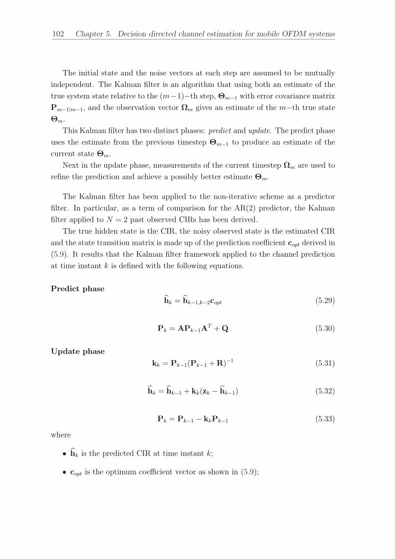
102 Chapter 5. Decision directed channel estimation for mobile OFDM systems
The initial state and the noise vectors at each step are assumed to be mutually
independent. The Kalman filter is an algorithm that using both an estimate of the
true system state relative to the (m−1)−th step, Θm−1 with error covariance matrix
Pm−1|m−1, and the observation vector Ωm gives an estimate of the m−th true state
Θm.
This Kalman filter has two distinct phases: predict and update. The predict phase
uses the estimate from the previous timestep Θm−1 to produce an estimate of the
current state Θm.
Next in the update phase, measurements of the current timestep Ωm are used to
refine the prediction and achieve a possibly better estimate Θm.
The Kalman filter has been applied to the non-iterative scheme as a predictor
filter. In particular, as a term of comparison for the AR(2) predictor, the Kalman
filter applied to N = 2 past observed CIRs has been derived.
The true hidden state is the CIR, the noisy observed state is the estimated CIR
and the state transition matrix is made up of the prediction coefficient copt derived in
(5.9). It results that the Kalman filter framework applied to the channel prediction
at time instant k is defined with the following equations.
Predict phase
hk = hk−1,k−2copt (5.29)
Pk = APk−1AT + Q (5.30)
Update phase
kk = Pk−1(Pk−1 + R)−1 (5.31)
hk = hk−1 + kk(zk − hk−1) (5.32)
Pk = Pk−1 − kkPk−1 (5.33)
where
• hk is the predicted CIR at time instant k;
• copt is the optimum coefficient vector as shown in (5.9);

5.4. Linear prediction 103
18 20 22 24 26 28 3010
−2
10−1
100
SNR [dB]
PE
R
Perfect CIRTD−LS non−iter.TD−LS non−iter. w/MMSE PredictorTD−LS non−iter. w/AR(2) PredictorTD−LS non−iter. w/Kalman Predictor
Figure 5.68: PER vs. SNR, DD-CE with Kalman filter - ETSI B, v = 120 km/h -
64-QAM 3/4, L = 2000 B
• hk−1,k−2 is the Lch × 2 matrix of the past predicted CIRs;
• A is the 2× 2 state transition matrix of the process where each column is the
vector ccopt;
• Pk is the 2× 2 estimate error covariance matrix;
• Q is the 2× 2 process noise covariance matrix with diagonal elements equal to
σ2hl
;
• kk is the 2× 2 Kalman gain matrix;
• zk is the observed (estimated) CIR.
Simulation results of PER vs. SNR shown in figures 5.68 to 5.70 for the three
worst cases selected in section 5.3.3 show the gain achieved by the Kalman filter
with reference to the DD-CE scheme with no predictor. Moreover a slightly gain in
performance can be seen with respect to the AR(2) predictor.
It should be noted that the Kalman filter leads to higher computational require-
ments with respect to the AR(2) predictor: the equations (5.29) to (5.33) are nec-
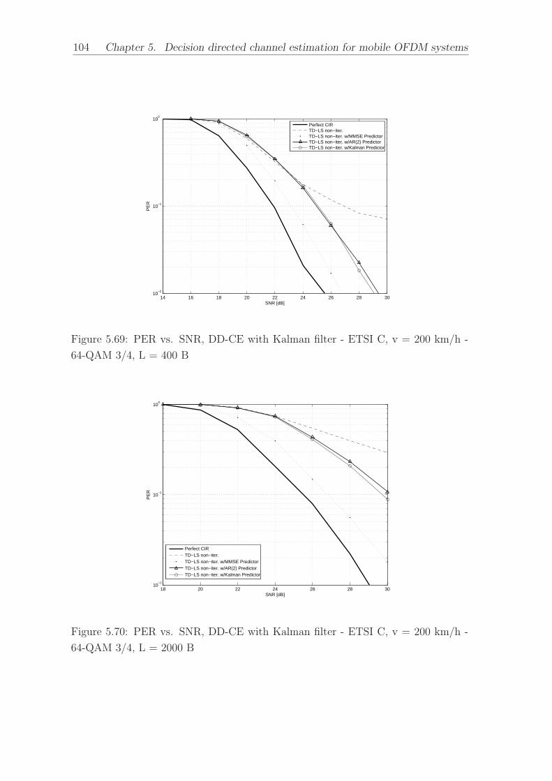
104 Chapter 5. Decision directed channel estimation for mobile OFDM systems
14 16 18 20 22 24 26 28 3010
−2
10−1
100
SNR [dB]
PE
R
Perfect CIRTD−LS non−iter.TD−LS non−iter. w/MMSE PredictorTD−LS non−iter. w/AR(2) PredictorTD−LS non−iter. w/Kalman Predictor
Figure 5.69: PER vs. SNR, DD-CE with Kalman filter - ETSI C, v = 200 km/h -
64-QAM 3/4, L = 400 B
18 20 22 24 26 28 3010
−2
10−1
100
SNR [dB]
PE
R
Perfect CIRTD−LS non−iter.TD−LS non−iter. w/MMSE PredictorTD−LS non−iter. w/AR(2) PredictorTD−LS non−iter. w/Kalman Predictor
Figure 5.70: PER vs. SNR, DD-CE with Kalman filter - ETSI C, v = 200 km/h -
64-QAM 3/4, L = 2000 B

5.4. Linear prediction 105
essary to implement the Kalman filter, on the contrary the AR(2) predictor makes
use only of the prediction phase (5.29).

106

Chapter 6
Doppler estimation techniques for
OFDM-based vehicular systems
Doppler effect estimation in vehicular systems can be important in order to deter-
mine a proper channel update refresh period, tailored to the relative speed between
transmitter and receiver. The well-known idea of DD-CE and tracking is that, in the
limit of static channel, one CE processing per packet, based on the initial preamble,
is sufficient while for non negligible vehicle speed CE tracking is required after an
initial CE instance.
The simulation results previously presented are related to the case of one CE
tracking update per each OFDM symbol, which can serve as lower bound on the
performance with respect to the CE tracking occurrence impact.
Aim of the investigations described in this section is to find out whether it is
possible to adaptively decrease the CE update period compared to the rate of the
input OFDM systems based on the relative speed between transmitter and receiver,
without significantly degrading the performance shown in the previous chapter.
This would be advantageous for power consumption and/or processing complexity
reduction of IEEE802.11p compliant receivers. A reliable relative speed estimation
must be accomplished in order to apply this idea. It could be objected that most
vehicular connectivity systems are envisioned to include GPS (satellite global posi-
tioning systems) apparatuses that can provide speed information reliably. However,
the required speed value is relative, so the two terminals should exchange speed
information. Moreover, the power consumption target would likely target portable
devices for which the GPS locator, if present, probably should not be always active.
In such cases baseband techniques for Doppler spread (and thus speed, intrinsically
107
108 Chapter 6. Doppler estimation techniques for OFDM-based vehicular systems
already relative between transmitter and receiver) estimation would likely be appeal-
ing for future vehicular conncetivity systems. The above considerations motivate the
assessment of the state-of-the-art Doppler spread estimation algorithms presented in
this chapter, and their application to vehicular systems.
6.1 Problem definition: impact of CE occurrence
on PHY performance
In this section the degradation of the channel estimate as a function of the speed
and the impact of CE occurrence on PER vs. SNR performance will be derived.
As shown in section 1.2.1, the wireless channel can be modeled as a WSS-US
process with Tc spaced taps defined as:
h(kT, nTc) =
Lch−1∑
l=0
hl(kT )δ(nTc − lTc) (6.1)
with Lch denoting the number of taps. It should be noted that the above equation
takes into account the US property of the hl(kT ) taps, l = 0, 1, . . . , Lch−1 and that,
in vehicular environment, the channel tap can be considered invariant within one
OFDM symbol period T for the typical relative speeds under consideration.
It can be shown that the related autocorrelation function is given by:
rh(∆t, ∆τ) = E[h(kT, τ)h∗(kT −∆t, τ −∆τ)
]=
Lch−1∑i=0
rhi(∆t)δ(∆τ − iTc) (6.2)
and
rhl(∆t) = E
[hl(kT )h∗l (kT −∆t)
]. (6.3)
By expressing the channel impulse response (6.1) in compact vectorial notation as
hk = [h0(kT ), h1(kT ), . . . , hLch−1(kT )]T , then the variation of the CIR at the time
instant kT with reference to the time (k − n)T canbe written:
∆hnk = hk − hk−n. (6.4)
As shown in [24] it results that the degradation ∆hnl,k of the l−th channel tap hl,k
at the time instant kT with reference to the l−th channel tap hl,k−n at time (k−n)T
can be estimated as:

6.1. Problem definition: impact of CE occurrence on PHY performance 109
E[∆hn
l,k∆h∗,nl,k
]= E
[(hl,k − hl,k−n
)(hl,k − hl,k−n
)∗]
= E[hl,kh
∗l,k − hl,khl,k−n − hl,k−nh
∗l,k + hl,k−nh
∗l,k−n
]
= E[hl,kh
∗l,k
]− E[hl,kh
∗l,k−n
]− E[hl,k−nh
∗l,k
]+ E
[hl,k−nh∗l,k−n
]
= 2 · (rhl(0)− rhl
(nT ))
(6.5)
then the MSE of the channel estimate introduced by the degradation of the channel
due to Doppler effect for a delay of n OFDM symbols is:
σ2d(n) = E
[‖∆hnk‖2]
= E [∆hn,∗k ∆hn,∗
k ]
=
Lch−1∑
l=0
2 · (rhl(0)− rhl
(nT ))
(6.6)
The Doppler spread that characterizes independently the l−th tap is the Fourier
transform of the autocorrelation function of the l−th channel tap:
Dl(f) =
+∞∫
−∞
rhl(∆t)e−j2πf∆tdt. (6.7)
As said in chapter 5, a suitable Doppler spectrum for vehicular environment is the
classical Jakes model defined in (1.11) and applied independently to every channel
tap, for which (6.3) becomes:
rhl(∆t) = σ2
hlJ0(2πfD∆t) (6.8)
being fD the Doppler spread and J0(z) the first order Bessel function of first kind.
Combining 6.6 with 6.8, σ2d(n) becomes:
σ2d(n) =
Lch−1∑
l=0
2 · (rhl(0)− rhl
(nT )) =
Lch−1∑
l=0
2 · σ2hl
(1− J0(2πfDnT )) (6.9)
If CE tracking is performed once every n OFDM symbols, i.e. Hk−n is used to
perform equalization of Yk instead of Hk, the mean estimation error e(n) experienced
for varying time instants from 1 to n can be evaluated as:
e(n) =1
n
n∑i=1
σ2d(i) =
2
n
n∑i=1
Lch−1∑
l=0
σ2hl
(1− J0(2πfDiT )) =2
n
n∑i=1
(1− J0(2πfDiT ))
(6.10)

110 Chapter 6. Doppler estimation techniques for OFDM-based vehicular systems
1 2 3 4 5 6 7 8 9 1010
−4
10−3
10−2
10−1
100
maximum estimation error e(n) as function of the period of channel tracking
Channel estimation period n [OFDM symbols]
e(n)
v = 60 km/hv = 120km/hv = 200km/h
Figure 6.1: Mean square error as function of the estimation period n and different
relative speeds
where the inner summation in (6.10) takes into account that the PDP of the channel
is usually normalized to 1, as shown in (1.20). e(n) is shown as a function of n in
figure 6.1, for three different relative speeds between transmitter and receiver.
In equation 6.9 the MSE of the channel estimate introduced by the degradation
of the channel for a delay of n OFDM symbols has been derived. It should be noted
that in static scenario the autocorrelation of the l−th channel tap is rhl(∆t) = σ2
hl
∀∆t ∈ R and no degradation occurs, i.e. σ2d(n) = 0 ∀n.
As shown in [24] the error introduced by the variation of the channel, for a delay
of n OFDM symbols, can be seen as an equivalent noise contribution at the receiver,
i.e. being σ2d(n) = E[‖∆hn(kT )‖2], then the equivalent SNR of the system as a
function of n is given by:
SNR′(n) =E[|An|2]
σ2w + σ2
d(n)(6.11)
where E[|An|2] is the signal energy and σ2w = N0 is the AWGN PSD.
In case the CE is updated once every n OFDM symbols, then (6.11) should be
6.1. Problem definition: impact of CE occurrence on PHY performance 111
evaluated for all the intermediate time instants j = 1, . . . , n and an average SNR
can be taken as an effective measure of the average experienced SNR. However,
a conservative measure given by (6.11) for the largest time instant only can be
taken as reference in order to determine a proper CE tracking interval and limit the
performance degradation. This will be better explained in the following.
Figures 6.2(a), 6.2(b) and 6.2(c) plot SNR′(n) versus the ideal SNR as a function
of different values for the relative speed v and for different CE tracking intervals n.
Such plots are important as they indicate a bound on the achievable effective SNR for
a given CE tracking interval. Based on them, a value for n can be chosen as a function
of speed and theoretical SNR range, once a maximum limit on the acceptable SNR
degradation is set by the designer.
A strategy to relate the value to different speeds is a threshold on the maximum
degradation introduced on SNR’ by σ2d(n).
For example, setting 1 dB as the maximum acceptable SNR degradation, the
resulting tolerable CE tracking interval n is reported in Table 6.1. The values have
been determined taking into account Figure 6.2 and three speed ranges having as mid-
range thresholds the speed values used for the PER vs. SNR simulations presented
in this work, i.e. v = 0, 60, 120, 200 km/h. For a speed v < 30 km/h the channel is
considered time-invariant and channel tracking is not performed.
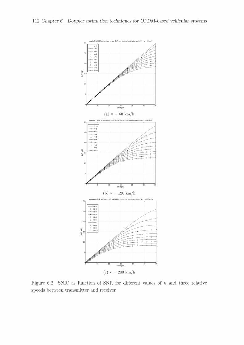
112 Chapter 6. Doppler estimation techniques for OFDM-based vehicular systems
0 5 10 15 20 25 300
5
10
15
20
25
30equivalent SNR as function of real SNR and channel estimation period N − v = 60km/h
SNR [dB]
SN
R‘ [
dB]
N =1
N=2
N=3
N=4
N=5
N=6
N=7
N=8
N=9
N=10
(a) v = 60 km/h
0 5 10 15 20 25 300
5
10
15
20
25
30equivalent SNR as function of real SNR and channel estimation period N − v = 120km/h
SNR [dB]
SN
R‘ [
dB]
N =1
N=2
N=3
N=4
N=5
N=6
N=7
N=8
N=9
N=10
(b) v = 120 km/h
0 5 10 15 20 25 300
5
10
15
20
25
30equivalent SNR as function of real SNR and channel estimation period N − v = 200km/h
SNR [dB]
SN
R‘ [
dB]
N =1
N=2
N=3
N=4
N=5
N=6
N=7
N=8
N=9
N=10
(c) v = 200 km/h
Figure 6.2: SNR’ as function of SNR for different values of n and three relative
speeds between transmitter and receiver

6.1. Problem definition: impact of CE occurrence on PHY performance 113
CE occurrence (n) n for n forSNR for 30 < v < 90 90 < v < 160 v > 160 km/h
km/h km/h
1 10 10 102 10 10 103 10 10 94 10 10 85 10 10 76 10 10 67 10 9 58 10 8 59 10 7 410 10 6 411 10 6 312 10 5 313 9 4 214 8 4 215 7 3 216 6 3 217 6 3 118 5 2 119 4 2 120 4 2 121 3 1 122 3 1 123 3 1 124 2 1 125 2 1 126 2 1 127 1 1 128 1 1 129 1 1 130 1 1 1
Table 6.1: CE tracking interval for 1 dB SNR degradation as a function of the
theoretical imposed SNR.

114 Chapter 6. Doppler estimation techniques for OFDM-based vehicular systems
6.2 Techniques for Doppler spread estimation
In order to be able to extrapolate an effective value of the channel estimation period
n, the relative speed between transmitter and receiver must be estimated.We recall
that the relative speed is directly related to the Doppler spread fD of the CIR as:
v =fDc
fc
(6.12)
where v is the relative speed expressed in [m/s], c is the speed of light and fc is the
carrier frequency. In literature a large number of Doppler spread estimators have
been proposed; these can be divided in two classes: one is based on level-crossing rate
(LCR) measurement of the considered process, the other is based on the estimation
of the auto-covariance function of the process [29], [30]. In vehicular environment the
main requirements for speed estimation are the robustness to noise, i.e. the ability
to track Doppler Spread even at low SNR, and low convergence time, derived from
the fast time-varying nature of the scenarios.
The Doppler Spread estimation method based on the zero-crossing rate (ZCR)
measurement [28] has been considered, that is a particular case of the LCR esti-
mators. The main advantage of this technique is the low complexity of its imple-
mentation, however it requires a very long convergence time. Another significant
investigated method based on the estimation of the autocorrelation function of the
channel is [29], which will be shown to provide good performance when applied to
IEEE 802.11p systems.
The next sections report the analysis of the mentioned Doppler spread estimators,
evaluation of their performance and effectiveness in vehicular environment.
6.2.1 Hybrid autocorrelation-based Doppler spread estima-
tor
This section refers to the algorithm proposed in [29]. It is based on the evaluation
of the autocorrelation of the CIR, and is named hybrid because it then uses the
autocorrelation estimate according to either a curvature estimator or a first zero
detection method, depending on the Doppler spread value range. The estimated
autocorrelation coefficient of the l−th tap of the CIR evaluated for a delay of m
6.2. Techniques for Doppler spread estimation 115
OFDM symbols is given by:
ρhl(mT ) =
1
(N −m)T
N−m∑i=1
hl(iT )h∗l (iT + mT )
1
N
N∑i=1
|hl(iT )|2(6.13)
where NT is the observation time, meaning that the estimate is performed consid-
ering N OFDM symbols. Despite in [29] the estimator is described as un-biased, for
real CE estimates hl one has:
σ2hl
= E[hlh∗l ] = E[(hl + nl)(hl + nl)
∗] ' 1
NT
N∑i=1
|hl(iT )|2 ' σ2hl
+ σ2nl
(6.14)
where nl has been defined as the CE error of the CIR at the l−th tap and σ2nl
=
E[|hl − hl|2] is the mean square error (MSE). Thus, (6.13) has been modified to
remove the bias thus obtaining:
ρhl(mT ) =
1
N −m
N−m∑i=1
hl(iT )h∗l ((i + m)T )
1
N
N∑i=1
|hl(iT )|2 − σ2nl
(6.15)
where it has been assumed that nl at different time instants is statistically indepen-
dent and thus does not affect the numerator on average.
The expression of the term σ2nl
depends on the employed CE technique. An
example is provided in chapter 4 with reference to the TD-LS and the modified
TD-LS RR of [15], in sections 4.1.2 and 4.1.3, respectively.
After estimating the normalized autocorrelation coefficient for every channel tap,
the method proposed in [29] improves the estimation accuracy by averaging the
normalized ρhl(mT ) for K taps:
ρh(mT ) =1
K
K∑
l=1
ρhl(mT ) (6.16)
An example of the behavior of ρh(mT ) estimator for a single channel realization
and tap combining with K = 1, . . . , 4 and m = 1 (we recall that T = 8µs), is
reported in figures 6.3(a) and 6.3(b) as a function of the estimation time expressed
in WLAN packets (16QAM 2000Byte packet length), for v = 60 km/h and v = 200
km/h respectively.
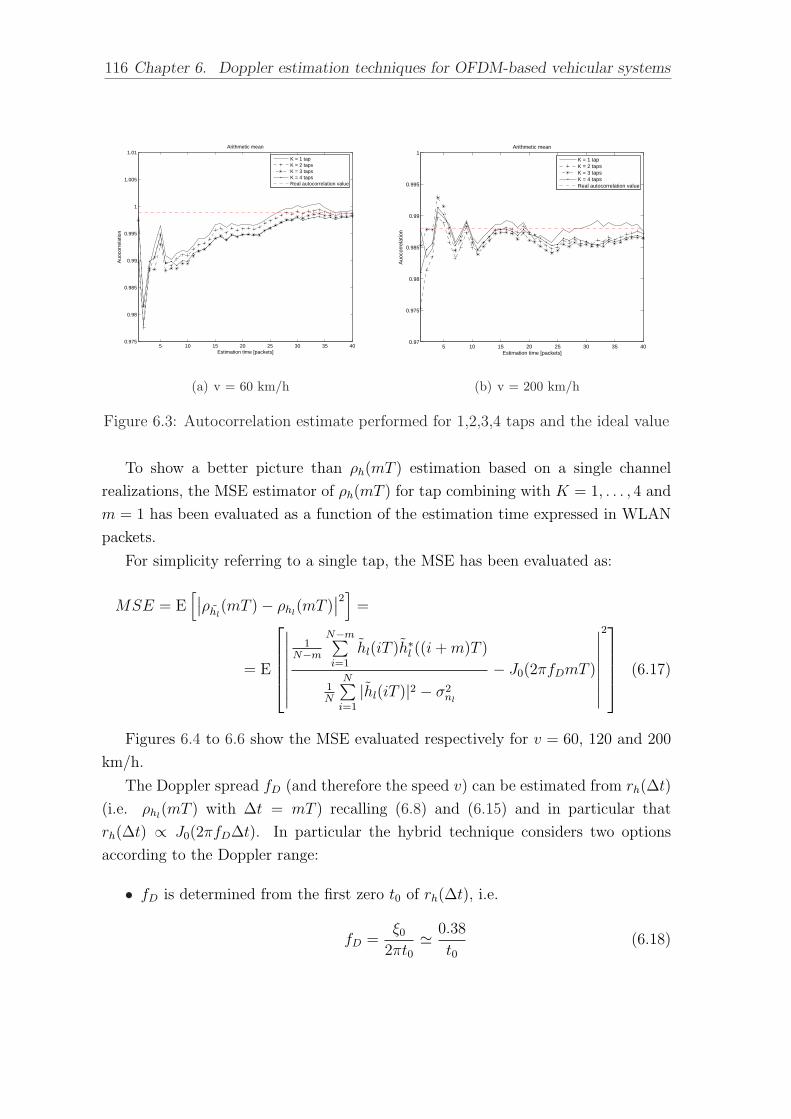
116 Chapter 6. Doppler estimation techniques for OFDM-based vehicular systems
5 10 15 20 25 30 35 400.975
0.98
0.985
0.99
0.995
1
1.005
1.01
Estimation time [packets]
Auo
corr
elat
ion
Arithmetic mean
K = 1 tapK = 2 tapsK = 3 tapsK = 4 tapsReal autocorrelation value
(a) v = 60 km/h
5 10 15 20 25 30 35 400.97
0.975
0.98
0.985
0.99
0.995
1
Estimation time [packets]
Auo
corr
elat
ion
Arithmetic mean
K = 1 tapK = 2 tapsK = 3 tapsK = 4 tapsReal autocorrelation value
(b) v = 200 km/h
Figure 6.3: Autocorrelation estimate performed for 1,2,3,4 taps and the ideal value
To show a better picture than ρh(mT ) estimation based on a single channel
realizations, the MSE estimator of ρh(mT ) for tap combining with K = 1, . . . , 4 and
m = 1 has been evaluated as a function of the estimation time expressed in WLAN
packets.
For simplicity referring to a single tap, the MSE has been evaluated as:
MSE = E[∣∣ρhl
(mT )− ρhl(mT )
∣∣2]
=
= E
∣∣∣∣∣∣∣∣
1N−m
N−m∑i=1
hl(iT )h∗l ((i + m)T )
1N
N∑i=1
|hl(iT )|2 − σ2nl
− J0(2πfDmT )
∣∣∣∣∣∣∣∣
2 (6.17)
Figures 6.4 to 6.6 show the MSE evaluated respectively for v = 60, 120 and 200
km/h.
The Doppler spread fD (and therefore the speed v) can be estimated from rh(∆t)
(i.e. ρhl(mT ) with ∆t = mT ) recalling (6.8) and (6.15) and in particular that
rh(∆t) ∝ J0(2πfD∆t). In particular the hybrid technique considers two options
according to the Doppler range:
• fD is determined from the first zero t0 of rh(∆t), i.e.
fD =ξ0
2πt0' 0.38
t0(6.18)

6.2. Techniques for Doppler spread estimation 117
1 2 3 4 5 6 7 8 9 1010
−6
10−5
10−4
10−3
MSE of autocorrelation estimated − v = 60km/h − Arithmetic mean
Estimation time [packets]
MS
E
1 tap2 taps3 taps4 taps
Figure 6.4: MSE of the autocorrelation values estimated, v = 60 km/h
1 2 3 4 5 6 7 8 9 1010
−6
10−5
10−4
10−3
Estimation time [packets]
MS
E
MSE of autocorrelation estimated − v = 120km/h − Arithmetic mean
1 tap2 taps3 taps4 taps
Figure 6.5: MSE of the autocorrelation values estimated, v = 120 km/h
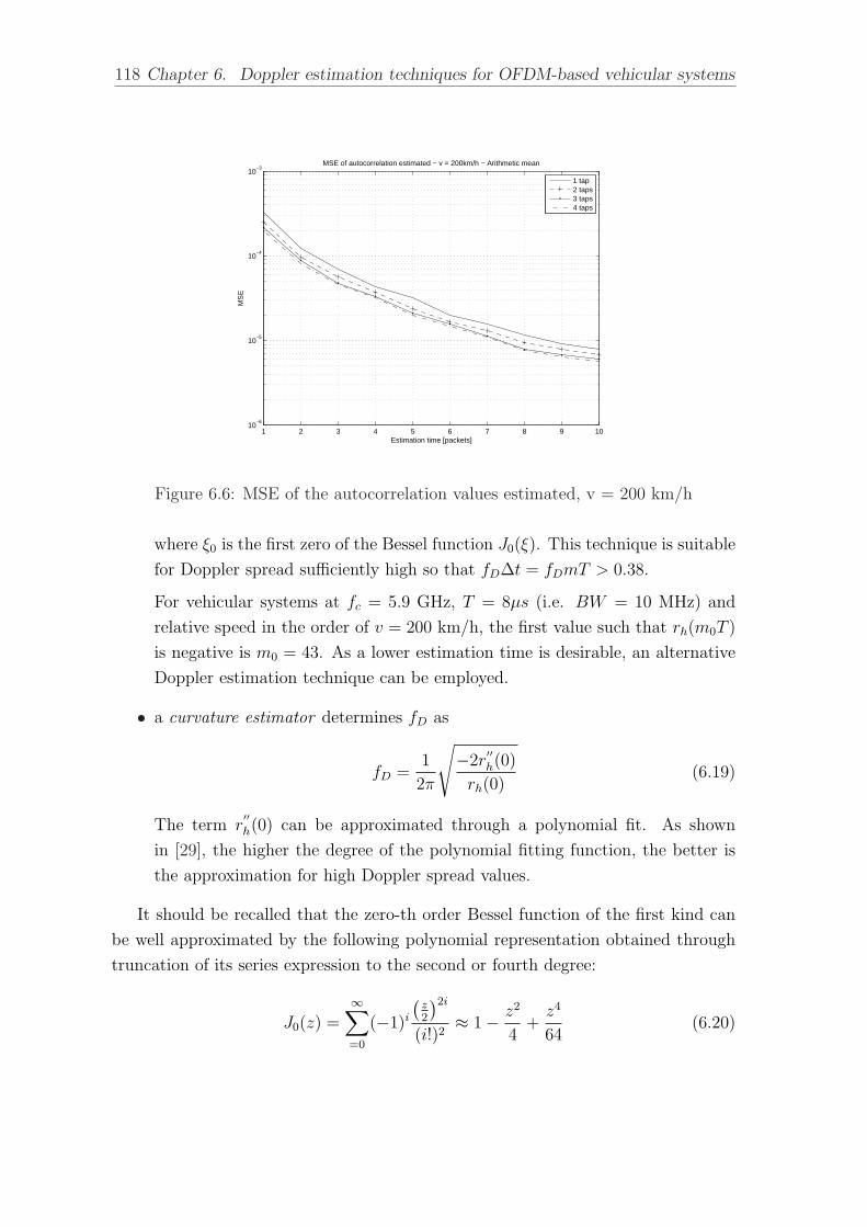
118 Chapter 6. Doppler estimation techniques for OFDM-based vehicular systems
1 2 3 4 5 6 7 8 9 1010
−6
10−5
10−4
10−3
Estimation time [packets]
MS
E
MSE of autocorrelation estimated − v = 200km/h − Arithmetic mean
1 tap2 taps3 taps4 taps
Figure 6.6: MSE of the autocorrelation values estimated, v = 200 km/h
where ξ0 is the first zero of the Bessel function J0(ξ). This technique is suitable
for Doppler spread sufficiently high so that fD∆t = fDmT > 0.38.
For vehicular systems at fc = 5.9 GHz, T = 8µs (i.e. BW = 10 MHz) and
relative speed in the order of v = 200 km/h, the first value such that rh(m0T )
is negative is m0 = 43. As a lower estimation time is desirable, an alternative
Doppler estimation technique can be employed.
• a curvature estimator determines fD as
fD =1
2π
√−2r
′′h(0)
rh(0)(6.19)
The term r′′h(0) can be approximated through a polynomial fit. As shown
in [29], the higher the degree of the polynomial fitting function, the better is
the approximation for high Doppler spread values.
It should be recalled that the zero-th order Bessel function of the first kind can
be well approximated by the following polynomial representation obtained through
truncation of its series expression to the second or fourth degree:
J0(z) =∞∑=0
(−1)i
(z2
)2i
(i!)2≈ 1− z2
4+
z4
64(6.20)

6.2. Techniques for Doppler spread estimation 119
0 2 4 6 8 10 12 14 16 18 200.97
0.975
0.98
0.985
0.99
0.995
1
1.005
m
φ(m
T)
Theoretical2nd degree4th degree
(a) v = 60 km/h
0 2 4 6 8 10 12 14 16 18 200.55
0.6
0.65
0.7
0.75
0.8
0.85
0.9
0.95
1
m
φ(m
T)
Theoretical2nd degree4th degree
(b) v = 200 km/h
Figure 6.7: Zero-th order Bessel function of first kind J0(2πfDmT ) and its approxi-
mation
Actually the fourth degree polynomial approximation is not required for the value
range of interest to us, as shown in Figure 6.7.
From (6.20) the general expression for the fourth order polynomial fit of rh(∆t),
based on the estimated discrete values rh(iT ), with i = 1, . . . , m, is given by:
p(x) = a0 + a2x2 + a4x
4, x =∆t
T(6.21)
In vector notation we define a = (a0, a2, a4)T , r = (rh(T ), . . . , rh(mT )) and p =
(p(1), p(2), . . . , p(m)) . It results that p = Ha is the system of equations of the
problem, where the matrix H has been defined as:
H =
1 1 1
1 22 24
......
...
1 m2 m4
(6.22)
The least square fit of r is a that minimizes ‖r−Ha‖2. It results that:
a = (HTH)−1HT r = Br (6.23)
where B = (HTH)−1HT .
For a k−th degree polynomial approximation only the first k entries of a can be
retained. Finally, for either k = 2 or k = 4 the Doppler spread estimate can be
obtained from (6.19) as:
fD =1
πT
√−a2
a0
(6.24)

120 Chapter 6. Doppler estimation techniques for OFDM-based vehicular systems
An alternative simplified estimate can also be obtained as follows. A reduced
vector r is considered, i.e. r = (rh(0), rh(mT )), m > 0, and considering a 2nd order
polynomial fit. It results that
H =
(1 0
1 m2
)(6.25)
and
B =
(1 0
−1/m2 1/m2
). (6.26)
From (6.23) the elements of the coefficient vector a are given by:
a0 = rh(0)
a2 = (−rh(0) + rh(mT ))/m2(6.27)
The result (6.27) can also be obtained considering the second order approximation
of rh(mT ):
rh(mT ) ≈ P (mT ) = a0 + a2m2. (6.28)
and derive the unknown coefficient estimates a0 and a2 as:
a0 = rh(0) (6.29)
a2 =rh(mT )− a0
m2(6.30)
Substituting (6.29) and (6.30) in (6.24) it results that the estimated Doppler
spread fD is:
fD =1
πT
√−a2
a0
=1
πmT
√rh(0)− rh(mT )
rh(0)(6.31)
Recalling that ρh(mT ) = rh(mT )/rh(0), fD can finally be expressed as:
fD =1
πmT
√rh(0)− ρh(mT )rh(0)
rh(0)=
√1− ρh(mT )
πmT. (6.32)
As reference the relative speed v has been estimated with both Doppler esti-
mators (6.24) and (6.32). The general fitting method was computed with rh(mT ),
m = 1, . . . , 10 and the simplified method with rh(0) and rh(mT ) , m = 1. The
considered simulation scenario was 16-QAM CR 1/2, 2000 B packet length, ETSI C
channel model; the estimated speeds are shown in figures 6.8(a) and 6.8(b). The CE
algorithm used is the TD-LS RR described in section 4.1.2.
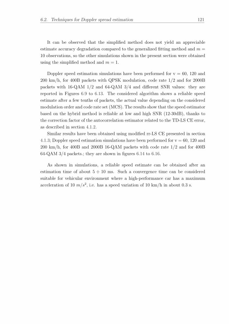
6.2. Techniques for Doppler spread estimation 121
It can be observed that the simplified method does not yield an appreciable
estimate accuracy degradation compared to the generalized fitting method and m =
10 observations, so the other simulations shown in the present section were obtained
using the simplified method and m = 1.
Doppler speed estimation simulations have been performed for v = 60, 120 and
200 km/h, for 400B packets with QPSK modulation, code rate 1/2 and for 2000B
packets with 16-QAM 1/2 and 64-QAM 3/4 and different SNR values: they are
reported in Figures 6.9 to 6.13. The considered algorithm shows a reliable speed
estimate after a few tenths of packets, the actual value depending on the considered
modulation order and code rate set (MCS). The results show that the speed estimator
based on the hybrid method is reliable at low and high SNR (12-30dB), thanks to
the correction factor of the autocorrelation estimator related to the TD-LS CE error,
as described in section 4.1.2.
Similar results have been obtained using modified rr-LS CE presented in section
4.1.3; Doppler speed estimation simulations have been performed for v = 60, 120 and
200 km/h, for 400B and 2000B 16-QAM packets with code rate 1/2 and for 400B
64-QAM 3/4 packets.; they are shown in figures 6.14 to 6.16.
As shown in simulations, a reliable speed estimate can be obtained after an
estimation time of about 5 ÷ 10 ms. Such a convergence time can be considered
suitable for vehicular environment where a high-performance car has a maximum
acceleration of 10 m/s2, i.e. has a speed variation of 10 km/h in about 0.3 s.

122 Chapter 6. Doppler estimation techniques for OFDM-based vehicular systems
10 20 30 40 50 60 70 80 90 1000
50
100
150
200
250
Estimation time [packets]
spee
d [k
m/h
]
Simplified methodHybrid method, m = 10real speed
(a) v = 60 km/h
10 20 30 40 50 60 70 80 90 1000
50
100
150
200
250
Estimation time [packets]
spee
d [k
m/h
]
Simplified methodHybrid method, m = 10real speed
(b) v = 200 km/h
Figure 6.8: Estimated speed with Hybrid and simplified methods
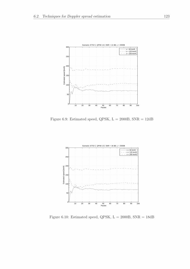
6.2. Techniques for Doppler spread estimation 123
10 20 30 40 50 60 70 80 90 1000
50
100
150
200
250
300
Packet
Est
imat
ed s
peed
[km
/h]
Scenario: ETSI C, QPSK 1/2, SNR = 12 dB, L = 2000B
v = 60 km/hv = 120 km/hv = 200 km/h
Figure 6.9: Estimated speed, QPSK, L = 2000B, SNR = 12dB
10 20 30 40 50 60 70 80 90 1000
50
100
150
200
250
300
Packet
Est
imat
ed s
peed
[km
/h]
Scenario: ETSI C, QPSK 1/2, SNR = 18 dB, L = 2000B
v = 60 km/hv = 120 km/hv = 200 km/h
Figure 6.10: Estimated speed, QPSK, L = 2000B, SNR = 18dB

124 Chapter 6. Doppler estimation techniques for OFDM-based vehicular systems
10 20 30 40 50 60 70 80 90 1000
50
100
150
200
250
300
Packet
Est
imat
ed s
peed
[km
/h]
Scenario: ETSI C, 16QAM 1/2, SNR = 18 dB, L = 2000B
v = 60 km/hv = 120 km/hv = 200 km/h
Figure 6.11: Estimated speed, 16-QAM, L = 2000B, SNR = 18dB
10 20 30 40 50 60 70 80 90 1000
50
100
150
200
250
300
Packet
Est
imat
ed s
peed
[km
/h]
Scenario: ETSI C, QPSK 1/2, SNR = 25 dB, L = 2000B
v = 60 km/hv = 120 km/hv = 200 km/h
Figure 6.12: Estimated speed, ETSI C, QPSK, L = 2000B, SNR = 25dB

6.2. Techniques for Doppler spread estimation 125
10 20 30 40 50 60 70 80 90 1000
50
100
150
200
250
300
Packet
Est
imat
ed s
peed
[km
/h]
Scenario: ETSI C, 64QAM 3/4, SNR = 30 dB, L = 2000B
v = 60 km/hv = 120 km/hv = 200 km/h
Figure 6.13: Estimated speed. ETSI C, 64-QAM, L = 2000B, SNR = 30dB
20 40 60 80 100 120 140 160 180 2000
50
100
150
200
250
Estimation time [packets]
Est
imat
ed s
peed
[km
/h]
Scenario: ETSI C, 16QAM 1/2, SNR = 18dB, L = 400B
v = 60 km/hv = 120 km/hv = 200 km/h
Figure 6.14: Estimated speed. ETSI C, 16-QAM 1/2, L = 400B, SNR = 18dB
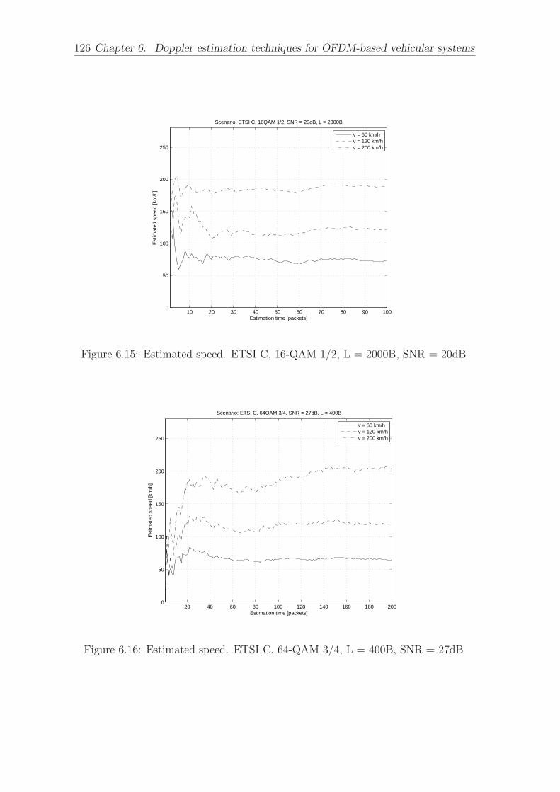
126 Chapter 6. Doppler estimation techniques for OFDM-based vehicular systems
10 20 30 40 50 60 70 80 90 1000
50
100
150
200
250
Scenario: ETSI C, 16QAM 1/2, SNR = 20dB, L = 2000B
Estimation time [packets]
Est
imat
ed s
peed
[km
/h]
v = 60 km/hv = 120 km/hv = 200 km/h
Figure 6.15: Estimated speed. ETSI C, 16-QAM 1/2, L = 2000B, SNR = 20dB
20 40 60 80 100 120 140 160 180 2000
50
100
150
200
250
Estimation time [packets]
Est
imat
ed s
peed
[km
/h]
Scenario: ETSI C, 64QAM 3/4, SNR = 27dB, L = 400B
v = 60 km/hv = 120 km/hv = 200 km/h
Figure 6.16: Estimated speed. ETSI C, 64-QAM 3/4, L = 400B, SNR = 27dB

6.2. Techniques for Doppler spread estimation 127
6.2.2 Doppler spread estimation based on ZCR measure-
ment
The second Doppler spread estimator evaluated is based on the estimation of the zero
crossing rate (ZCR) of the channel taps [28]; the ZCR of a differentiable stationary
random process is the average number of zero-crossing event in the unitary time.
Being S(f) the Power Spectral density of the process, the ZCR η in the unitary time
results [28]:
η2 =−r′′(0)
π2r(0)=
+∞∫−∞
ω2S(ω)dω
π2+∞∫−∞
S(ω)dω
(6.33)
where r(∆τ) is the autocorrelation function of the process evaluated for a delay ∆τ .
Applying the Classical Jakes spectrum model defined in (1.11) to the equation 6.33,
it results:
η2 = 2f 2D. (6.34)
The presence of noise in the process reflects in a bias estimate of fD when inverting
(6.34); in other words, as shown in chapter 4, the AWGN noise that introduces an
estimation error in the channel estimate, causes a bias estimate of fD. The authors
in [28] introduces a correcting factor to take into account the influence of the noise
in the channel estimate; the unbiased estimate results:
I(2)D = η2π2 − I
(2)N − η2π2I
(0)N
2SNR(6.35)
where SNR is the signal-to-noise ratio seen by the channel impulse response and the
terms I(0)N and I
(2)N are defined as:
I(n)N =
+∞∫
−∞
ωn|H(ω)|2dω, (6.36)
being H(ω) the low-pass filter transfer function of the receiver equipment. The
relation between I(2)D and the estimated Doppler Spread is fD:
fD =1
π
√1
2I
(2)D . (6.37)

128 Chapter 6. Doppler estimation techniques for OFDM-based vehicular systems
Speed [km/h] Doppler spread fD
[Hz]
ZCR η ZCR in the OFDM
symbol time (ηT )
60 327 231 0.0018
120 655 463 0.0037
200 1092 772 0.0061
Table 6.2: Theoretical ZCR in absence of noise
From equation (6.34) the ZCR in absence of noise can be estimated for given
Doppler frequencies, as reported in table 6.2. It should be recalled that the Doppler
Spread is fD = fcv/c with carrier frequency fc = 5.9 GHz and the symbol time T is
T = 8µs.
From table 6.2 it can be noted the mean time expected to see a minimum amount
of zero-crossing events necessary to achieve a reliable ZCR estimation. For example
the mean number of OFDM symbols expected to see 20 zero-crossing events at v = 60
km/h is N = 5550, that corresponds to ' 70 16-QAM 1/2 L = 2000B packets.
This example clarifies that the convergence time of the ZCR method is significantly
larger than the hybrid method above described, as confirmed by the simulations
results reported in 6.17 to 6.19 and obtained by measuring the actual ZCR of the
estimated channel taps (given in practice by the number of times the sign changes
from positive to negative) for a single channel realization with its time evolution
given by the Doppler effect. It should also be noted that the estimator accuracy is
highly susceptible to noise, as shown in 6.19 where the behavior is comparable to the
plots obtained with the hybrid autocorrelation based method but with a high SNR
such as 40 dB.
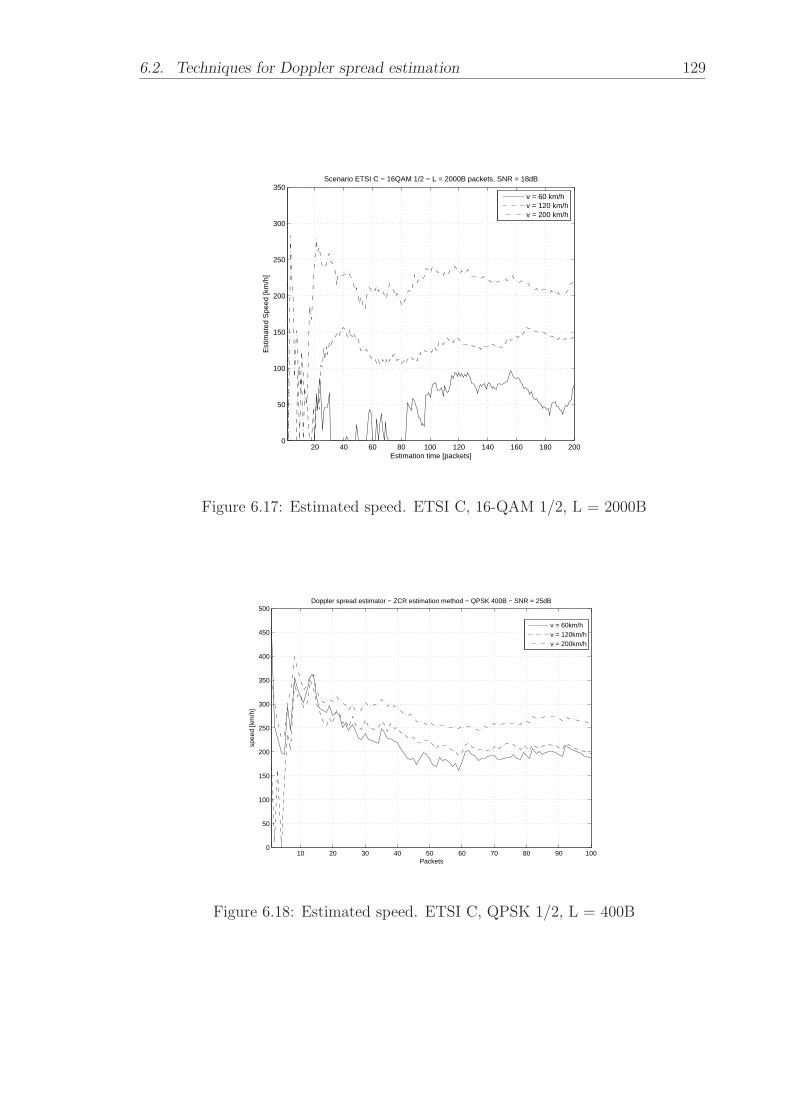
6.2. Techniques for Doppler spread estimation 129
20 40 60 80 100 120 140 160 180 2000
50
100
150
200
250
300
350Scenario ETSI C − 16QAM 1/2 − L = 2000B packets, SNR = 18dB
Estimation time [packets]
Est
imat
ed S
peed
[km
/h]
v = 60 km/hv = 120 km/hv = 200 km/h
Figure 6.17: Estimated speed. ETSI C, 16-QAM 1/2, L = 2000B
10 20 30 40 50 60 70 80 90 1000
50
100
150
200
250
300
350
400
450
500
Packets
spee
d [k
m/h
]
Doppler spread estimator − ZCR estimation method − QPSK 400B − SNR = 25dB
v = 60km/hv = 120km/hv = 200km/h
Figure 6.18: Estimated speed. ETSI C, QPSK 1/2, L = 400B

130 Chapter 6. Doppler estimation techniques for OFDM-based vehicular systems
10 20 30 40 50 60 70 80 90 1000
50
100
150
200
250
300
Estimation time [packets]
Est
imat
ed S
peed
[km
/h]
Scenario ETSI C − 16QAM 1/2 − L = 2000B packets, SNR = 40dB
v = 60 km/hv = 120 km/hv = 200 km/h
Figure 6.19: Estimated speed. ETSI C, 16-QAM 1/2, L = 2000B, SNR = 40dB

6.3. Performance curves with variable CE occurrence 131
In conclusion, the ZCR based technique [28] performs worse than then the hy-
brid autocorrelation based estimator [29] regarding the Doppler spread estimation
accuracy at low SNR and the required convergence speed, when applied to vehicu-
lar systems. The motivation is due to the characteristics of the system under focus
and the related Doppler spread ranges (depending on the carrier frequency and the
vehicle speed, as well known).
The only possible advantage of the ZCR estimator compared to the autocorrela-
tion based one is represented by its lower complexity and lower amount of data to
be processed, but this is not accompanied to an adequate estimation accuracy for
vehicular system Doppler spread values.
6.3 Performance curves with variable CE occur-
rence
The procedure used to evaluate the effectiveness of the algorithm that estimates the
Doppler spread for the considered system is the following:
1. Initially channel tracking is performed for every OFDM symbol with the TD-LS
reduced-rank Viterbi FEC technique;
2. during a period of time equivalent to P (table 6.4) transmitted packets the
Doppler estimator based on autocorrelation function performs the estimate
and the Doppler spread measured at the end of this period is returned;
3. the relative speed is derived from the Doppler spread measured as v = fDcfc
;
4. the CE period n is selected as proposed in table 6.3;
5. from packet P + 1 onwards, the CE is performed every n symbols.
From simulations on the estimated speed a minimum estimation period can be
set to achieve a reliable estimated speed. In table 6.4 the selected number of pack-
ets P has been reported for the various scenarios in which the estimation speed is
performed. The equivalent estimation time for the selected values of P is ≈ 5 ÷ 10
ms. Simulations have been performed for QPSK 1/2 L = 400B, 16-QAM 1/2 L =
2000B and 64-QAM 3/4 L = 400 B packets.
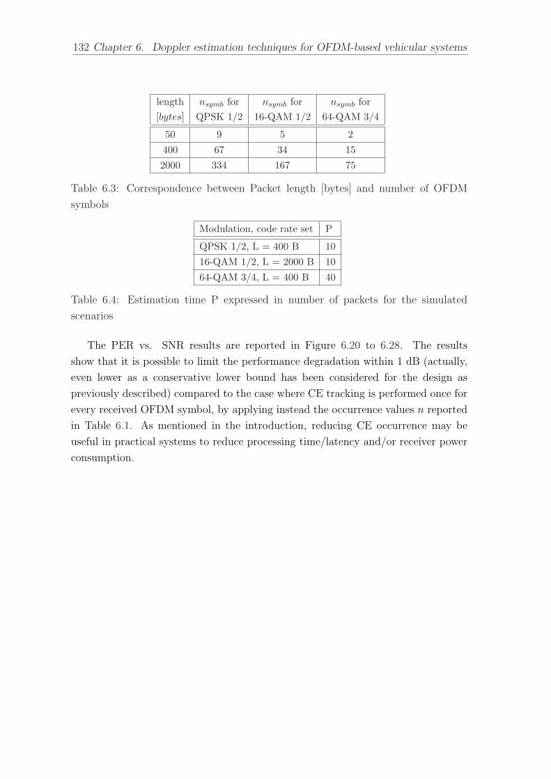
132 Chapter 6. Doppler estimation techniques for OFDM-based vehicular systems
length nsymb for nsymb for nsymb for[bytes] QPSK 1/2 16-QAM 1/2 64-QAM 3/4
50 9 5 2
400 67 34 15
2000 334 167 75
Table 6.3: Correspondence between Packet length [bytes] and number of OFDM
symbols
Modulation, code rate set P
QPSK 1/2, L = 400 B 10
16-QAM 1/2, L = 2000 B 10
64-QAM 3/4, L = 400 B 40
Table 6.4: Estimation time P expressed in number of packets for the simulated
scenarios
The PER vs. SNR results are reported in Figure 6.20 to 6.28. The results
show that it is possible to limit the performance degradation within 1 dB (actually,
even lower as a conservative lower bound has been considered for the design as
previously described) compared to the case where CE tracking is performed once for
every received OFDM symbol, by applying instead the occurrence values n reported
in Table 6.1. As mentioned in the introduction, reducing CE occurrence may be
useful in practical systems to reduce processing time/latency and/or receiver power
consumption.

6.3. Performance curves with variable CE occurrence 133
0 2 4 6 8 10 12 14 16 18 20 22 24 2610
−2
10−1
100
SNR [dB]
PE
R
Perfect CIRTD−LS, n = 1TD−LS w/Doppler estim.
Figure 6.20: PER vs. SNR. QPSK 1/2, L=400B, v = 60 km/h, reduced CE occur-
rance
0 2 4 6 8 10 12 14 16 18 20 22 24 26 28 3010
−2
10−1
100
SNR
PE
R
Perfect CIRTD−LS, n = 1TD−LS w/Doppler estim.
Figure 6.21: PER vs. SNR. QPSK 1/2, L=400B, v = 120 km/h, reduced CE occur-
rance

134 Chapter 6. Doppler estimation techniques for OFDM-based vehicular systems
0 2 4 6 8 10 12 14 16 18 20 22 24 26 28 3010
−2
10−1
100
SNR [dB]
PE
R
Perfect CIRTD−LS, n = 1TD−LS w/Doppler estim.
Figure 6.22: PER vs. SNR. QPSK 1/2, L=400B, v = 200 km/h, reduced CE occur-
rance
8 10 12 14 16 18 20 22 24 26 28 3010
−2
10−1
100
SNR [dB]
PE
R
Perfect CIRTD−LS, n = 1TD−LS w/Doppler estim.
Figure 6.23: PER vs. SNR. 16-QAM 1/2, L=2000B, v = 60 km/h, reduced CE
occurrance

6.3. Performance curves with variable CE occurrence 135
10 12 14 16 18 20 22 24 26 28 3010
−2
10−1
100
SNR
PE
R
Perfect CIRTD−LS, n = 1TD−LS w/Doppler estim.
Figure 6.24: PER vs. SNR. 16-QAM 1/2, L=2000B, v = 120 km/h, reduced CE
occurrance
8 10 12 14 16 18 20 22 24 26 28 3010
−2
10−1
100
SNR [dB]
PE
R
Perfect CIRTD−LS, n = 1TD−LS w/Doppler estim.
Figure 6.25: PER vs. SNR. 16-QAM 1/2, L=2000B, v = 200 km/h, reduced CE
occurrance

136 Chapter 6. Doppler estimation techniques for OFDM-based vehicular systems
14 16 18 20 22 24 26 28 3010
−2
10−1
100
SNR [dB]
PE
R
Perfect CIRTD−LS, n = 1TD−LS w/Doppler estim.
Figure 6.26: PER vs. SNR. 64-QAM 3/4, L=400B, v = 60 km/h, n reduced CE
occurrance
14 16 18 20 22 24 26 28 3010
−2
10−1
100
SNR
PE
R
Perfect CIRTD−LS, n = 1TD−LS w/Doppler estim.
Figure 6.27: PER vs. SNR. 64-QAM 3/4, L=400B, v = 120 km/h, reduced CE
occurrance

6.3. Performance curves with variable CE occurrence 137
14 16 18 20 22 24 26 28 3010
−2
10−1
100
SNR [dB]
PE
R
Perfect CIRTD−LS, n = 1TD−LS w/Doppler estim.
Figure 6.28: PER vs. SNR. 64-QAM 3/4, L=400B, v = 200 km/h, reduced CE
occurrance

138

Chapter 7
Conclusions
In this thesis data decoding-aided channel estimation techniques for OFDM sys-
tems in vehicular environment have been studied. The wireless channel in vehicular
environment exhibits a time-varying nature due to the relative speed between the
transmitter and the receiver, known as Doppler effect. It has been shown that, for
IEEE 802.11p systems, the initial channel estimation based on the standard pream-
ble must be updated several times per WLAN packet (each one composed of many
OFDM symbols) because of the degradation due to the Doppler effect.
Two different data-decoding aided CE schemes have been proposed:
• an iterative Viterbi decoding-aided DD-CE scheme, that make use of the
Viterbi decoder to decode the received symbols and reconstruct the transmitter
symbols that are used to perform the CE. After the CE has been updated the
received data are equalized for a second and final time using the updated CE
and finally decoded.
• a non-iterative Viterbi decoding-aided DD-CE scheme that is characterized by
lower complexity and latency compared to the iterative scheme: the decoded
bit stream are used at the same time for both the CE task and as final output
bit stream. It results that the Viterbi decoder, that is a very computationally
intensive block, is used only once per received symbol.
Simulation results show that the two presented schemes have almost the same perfor-
mance in most scenarios, and that both are able to track the channel very efficiently
for most considered channel and mobility scenarios, as shown by the comparison
with the ideally known channel for every received OFDM symbol.
139
140 Chapter 7. Conclusions
Despite that, two further improvements to the investigated channel tracking al-
gorithms have been evaluated. The first, was motivated by the performance gap
still observable compared to the ideal case for very challenging scenarios like high
relative speed (≥ 120 Km/h), long WLAN packets (≥ 400 byte), high modulation
orders (64-QAM). Linear prediction of the channel estimate has been considered in
order to provide a delay-free channel estimation to the equalization instance of the
OFDM symbol under focus: the MMSE linear prediction has been analyzed as a
term of comparison for the other sub-optimal predictors, being the MMSE predictor
practically unfeasible for the considered system due to the high computational re-
quirements and the always increasing memory requirements. The performance gain
achievable with the AR(2) predictor has been demonstrated compared to the scheme
without predictor and to the scheme featuring an MMSE predictor.
As second improvement to the data decoding-aided DD-CE scheme, the selection
of the CE occurrence as a function of the estimated relative speed between trans-
mitter and receiver has been presented. This may be useful in practical portable
systems to reduce processing time and/or power consumption. A strategy to select
the CE occurrence based on the relative speed between transmitter and receiver and
a maximum (set a-priori by the designer) tolerable degradation of the SNR seen at
the receiver, due to the Doppler effect, has been presented.
This idea can applied if reliable relative speed estimates are available at the re-
ceiver. It could be objected that most vehicular connectivity systems are envisioned
to include GPS (satellite global positioning systems) apparatuses that can provide
speed information reliably. However, relative speed information is needed so the two
terminals should exchange absolute speed information. Besides, the power consump-
tion reduction target would likely be meaningful for portable devices, for which the
GPS locator, if present, probably should not be always active. Therefore we deem
that baseband techniques for Doppler spread estimation can be appealing for future
vehicular connectivity systems. The above considerations motivated the assessment
of the state-of-the-art Doppler spread estimation algorithms and their application
to vehicular systems. Two different Doppler spread estimators have been analyzed
and compared. The Doppler spread estimator based on the autocorrelation function
estimation has proven to be the most suitable for IEEE 802.11p.
Finally, the PER vs. SNR simulation results with reduced CE occurrence based
on the estimated Doppler spread obtained using the mentioned selected relative
speed estimator, show that is possible to limit the SNR performance degradation

141
within a desired limit (for example, 1 dB) compared to the case where CE tracking
is performed once for every received OFDM symbol, by reducing significantly the
CE occurrence for a wide range of SNR values (in turn dependent on the estimated
relative speed).

142

Bibliography
[1] N. Benvenuto, G. Cherubini, Algorithms for Communications Systems and their
Applications, John Wiley & Sons, England, 2002.
[2] A. Goldsmith, Wireless communications, Cambridge University Press, 2005.
[3] IEEE P802.11pTM/D9.0, “Part 11: Wireless LAN Medium Access Control
(MAC) and Physical Layer (PHY) specifications”, Amendment 7: Wireless Ac-
cess in Vehicular Environments, Sep. 2009.
[4] IEEE 802.11a-1999 Standard, “Part 11: Wireless LAN Medium Access Control
(MAC) and Physical Layer (PHY) Specifications: High-speed Physical Layer in
the 5 GHz Ban”, 1999.
[5] M. A. Ingram, G. Acosta, L. Dong, “Small-Scale Fading Models for the IEEE
802.11p (WAVE/DSRC) Standard”, School of Electrical and Computer Engi-
neering Georgia Institute of Technology Atlanta, Sep. 2006.
[6] J. Medbo, “Radio Wave Propagation Characterisitcs at 5 GHz with Modeling
Suggestion for HIPERLAN/2”, ETSI EP BRAN, Jan. 1998.
[7] J. Medbo, P. Schramm, “Channel Model for HIPERLAN/2 in Different Indoor
Scenarios”, ETSI EP BRAN, Mar. 1998.
[8] Y. G. Li and L. J. Crimini Jr., “Bounds on the interchannel interference of
OFDM in time-varying impairments”, IEEE Transactions on Communications,
vol. 49, no. 3, Mar. 2001.
[9] L. Wei, C. Ming, S. Cheng, H. Wang, “A complexity reduced blind channel
equalization scheme for OFDM systems”, IEEE 17th International Symposium
on Personal, Indoor and Mobile Radio Communications, 2006.
143

144 Bibliography
[10] R. Boloix-Tortosa, F. J. Simois-Tirado, J. J. Murillo-Fuentes, “Blind adaptive
channel estimation for OFDM systems”, IEEE 10th Workshop on Signal Pro-
cessing Advances in Wireless Communications, Jun. 2009.
[11] W. Yang, Y. Cai, Y. Xun, “Semi-blind Channel Estimation for OFDM Systems”,
IEEE 63rd Vehicular Technology Conference, May 2006.
[12] E. G. Larsson, G. Liu, J. Li, G. B. Giannakis, “Joint Symbol Timing and
Channel Estimate for OFDM Based WLANs,” IEEE Commun. Letters, vol. 5,
Aug. 2001.
[13] S. Ohno, G. B. Giannakis, “Optimal training and redundant precoding for block
transmissions with application to wireless OFDM”, IEEE Transactions on Com-
munications, vol. 50, no. 12, Dec. 2002.
[14] M. Hsieh, C. Wei, “Channel estimation for OFDM systems based on comb-type
pilot arrangement in frequency selective fading channels”, IEEE Transactions
on Consumer Electronics, Feb. 1998.
[15] E. Dall’Anese, A. Assalini, S. Pupolin, “On Reduced-rank Channel Estimation
and Prediction for OFDM-based Systems”, in Proc. WPMC ’07, Jaipur, India,
Dec. 2007.
[16] S. Kalyani, K. Giridhar, “Mitigation of Error Propagation in Decision Directed
OFDM Channel Tracking Using Generalized M Estimators”, IEEE Transactions
on Signal Processing, vol. 55, no. 5, May 2007.
[17] M. Siti, A. Assalini, E. Dall’Anese, S. Pupolin, “Low Complexity Decision-
Directed Channel Estimation based on a Reliable-Symbol Selection Strategy for
OFDM Systems”, To Appear: IEEE International Conference on Communica-
tions - Workshop on Vehicular Connectivity, May 2010.
[18] H. Abdulhamid, E. Abdel-Raheem and K.E. Tepe, “Channel estimation for 5.9
GHz dedicated short range communications receiver in wireless access vehicular
environments”, IET Communication, Dec. 2007.
[19] Q. Yuan, C. He, K. Ding, W. Bai, Z. Bu, “Channel Estimation and Equal-
ization for OFDM System with Fast Fading Channels”, IEEE 60th Vehicular
Technology Conference, 2004.
Bibliography 145
[20] T. Kella, “Decision-Directed Channel Estimation for Supporting Higher Ter-
minal Velocities in OFDM Based WLANs”, IEEE Global Telecommunications
Conference, 2003, GLOBECOM 2003.
[21] B. Ozbek, D. Le Ruyet, C. Panazio, “Pilot-Symbol-Aided iterative channel esti-
mation for OFDM-based Systems”, Conservatoire National des Arts et Metiers,
Aug. 2005.
[22] L. Jarbot, “Combined decoding and channel estimation of OFDM Systems in
Mobile Radio Networks”, IEEE 47th Vehicular Technology Conference, May
1997.
[23] J. Wee, W. Jeon, Y. Lee, K. Kwon, Y. Cho, “Pilot and Data Aided Channel
Estimation for OFDM systems in Rapidly Time-Varying Channels”, IEEE 69th
Vehicular Technology Conference, 2009. VTC Spring 2009.
[24] E. Dall’Anese, A. Assalini, S. Pupolin, “Enhanced multicarrier radio receiving
method for Vehicular Mobile Wideband Channel”, Internal report, Oct 2008.
[25] B. Moision, “A Truncation Depth Rule of thumb for Convolutional Codes”,
Information Theory and Applications Workshop, Jan. 2008.
[26] K. E. Baddour, N. C. Beaulieu, “Autoregressive modelling for Fading Channel
simulation”, IEEE Transaction on Communications, Jul. 2005.
[27] K. Han, S. Lee, J. Lim, K. Sung, “Channel Estimation for OFDM with Fast Fad-
ing Channels by Modified Kalman Filter”, IEEE Trans. Consumer Electronics,
May 2004.
[28] S. Valle, “Doppler spread measurements for tuning pilot-assisted channel es-
timation”, Proceedings of the 3rd IEEE International Symposium on Signal
Processing and Information Technology, 2003. ISSPIT 2003.
[29] O. Mauritz, “A Hybrid Method for Doppler Spread Estimation”, VTC 2004-
Spring. 2004 IEEE 59th Vehicular Technology Conference, 2004.
[30] L. Qiaoli, C. Wei, X. Tao, L. Biqi, “A Doppler Spread Estimator Design for
Mobile OFDM Systems”, ICCS 2008. 11th IEEE Singapore International Con-
ference on Communication Systems, 2008.

146