OF BOUNDARY ELEMENT METHODS G.A. CHANDLER

62

DISCRETE NORMS l!'OR THE CONVERGENCE

OF BOUNDARY ELEMENT METHODS

G.A. CHANDLER

1. INTRODUCTION.

The simplest of elliptic problems is the interior Dirichlet problem for Laplace's equa-

tion. We are given a bounded region Q c IR2 with a smooth boundary r, and want to

find the unknown function U satisfying

-t.U(x)=O, xEil, and

U(x)=g(x), xEr;

for some given function g.

As the fundamental solution for -t. is

G . ' 1 1 1 (x,~) :=- og-1 -,.1' 271' .x- <;;

we have Green's formula

(1.1) I Jr

.)Uv-;; G(x, .)U = U(x), x E int(Q)

(1.2) 1 . ) = -U(x , 2

x E r-.

(For any X E r, v(x) is the outward normal at x, Uv(x) = v(x).'VU(x), and Gv(x,O =

v(~).'VeG(x,~) is the normal derivative of G with respect to the second variable.) The

This work was supported by the Australian Research Council through the program grant Numerical analysis for integrals, integra./ equations and boundary value problems.

63

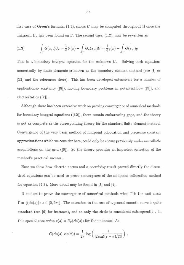
first case of Green's formula, (1.1), shows U may be computed throughout nonce the

unknown Uv has been found on r. The second case, (1.2), may be rewritten as

(1.3) lr G(x, .)Uv = ~U(x) -fr G11 (x, .)U = ~g(x) -fr G(x, .)g

This is a boundary integral equation for the unknown U11 • Solving such equations

numerically by finite elements is known as the boundary element method (see [1] or.

[12] and the references there). This has been developed extensively for a number of

applications:- elasticity ([8]), moving boundary problems in potential fiow ([9]), and

electrostatics ([7]).

Although there has been extensive work on proving convergence of numerical methoda

for boundary integral equations ([12]), there remain embarassing gaps, and the theory

is not as complete as the corresponding theory for the standard finite element method.

Convergence of the very basic method of midpoint collocation and piecewise constant

approximations which we consider here, could only be shown previously under unrealistic

assumptions on the grid ([6]). So the theory provides an imperfect reflection of the

method's practical success.

Here we show how discrete norms and a coercivity result proved directly the discre

tised equations can be used to prove convergence of the midpoint collocation method

for equation (1.3). More detail may be found in [3] and [4].

It suffices to prove the convergence of numerical methods when r is the unit circle

r = {( cis(s)) : s E [0, 21r]}. The extension to the case of a general smooth curve is quite'

standard (see [6] for instance), and so only the circle is considered subsequently . In

this special case write v(s) = U11 (cis(s)) for the unknown. As

G(cis(s),cis(cr)) = 2~ log C2sin((s 1_ cr)/2)1)

64

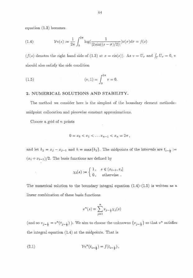
equation (1.3) becomes

(1.4)

(f(s) denotes the right hand side of (1.3) at x = cis(s)). As v = Uv and Jr Uv = 0, v

should also satisfy the side condition

(1.5) t" (v,1)= Jo v=O.

2. NUMERICAl" SOLUTIONS AND STABILITY.

The method we consider here is the simplest of the boundary element methods:-

midpoint collocation and piecewise constant approximations.

Choose a grid of n points

0 = Xo < X1 < ... Xn-1 < Xn = 27r,

and let hj = Xj- Xj-l and h = rnax{hj}· The midpoints of the intervals are ti-t .-

(x; + .Xi-I)/2. The basis functions are defined by

x;(s):= { 1'

' 0' otherwise

The numerical solution to the boundary integral equation (1.4)-(1.5) is written as a

linear combination of these basis functions

n

vn(s) = :;[ vj-!.\:i(s) j=l

(and so vj-~ = v"(tj-~) ). We aim to choose the unknowns {vj-~} so that v" satisfies

the integra.l equation (1.4) at the midpoints. That is

(2.1)

65

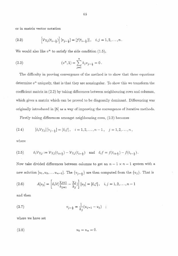
or in matrix vector notation

(2.2)

We would also like vn to satisfy the side condition (1.5),

n

(2.3) (vn,1) = Lhivj-~ = 0. j=l

The difficulty in proving convergence of the method is to show that these equations

determine vn uniquely, that is that they are nonsingular. To show this we transform the

coefficient matrix in (2.2) by taking differences between neighbouring rows and columns,

which gives a matrix which can be proved to be diagonally dominant. Differencing was

originally introduced in [5] as a way of improving the convergence of iterative methods.

Firstly taking differences amongst neighbouring rows, (2.2) becomes

(2.4) [o;Vxil [vi-~]= [o;J], i = 1,2, ... ,n -1, j = 1,2, ... ,n,

where

(2.5)

Now take divided differences between columns to get an n- 1 X n- 1 system with a

new solution [u1 ,u2 , ••• un-1 ]. The {vi-!} are then computed from the {uj}· That is

(2.6) i,j = 1,2, ... ,n -1

and then

(2.7)

where we have set

(2.8) uo = Un = 0.

66

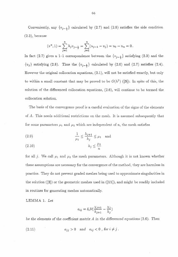
Conveniently, any { vi-t} calculated by (2. 7) and (2.8) satisfies the side condition

(2.3), because

n n

(vn, 1) = I:>jVj-~ = :Z:)·uj-1- Uj) = uo -- Un = 0. j=l j=l

In fact (2. 7) gives a 1-1 correspondence between the { vj- ~} satisfying (2.3) and the

{uj} satisfying (2.8). Thus the {vj-t} calculated by (2.6) and (2.7) satisfies (2.4).

However the original collocation equations, (2.1), will not be satisfied exactly, but only

to within a small constant that may be proved to be O(h2 ) ([3]). In spite of this, the

solution of the differenced collocation equations, (2.6), will continue to be termed the

collocation solution.

The basis of the convergence proof is a careful evaluation of the signs of the elements

of A. This needs additional restrictions on the mesh. It is assumed subsequently that

for some parameters p 1 and f-l 2 which are independent of n, the mesh satisfies

(2.9)

(2.10)

for all j. We call p 1 and p 2 the mesh parameters. Although it is not known whether

these assumptions are necessary for the convergence of the method, they are harmless in

practice. They do not prevent graded meshes being used to approximate singularities in

the solution ([2]) or the geometric meshes used in ([11]), and might be readily included

in routines for generating meshes automatically.

LEMMA 1. Let

aij = 8; V(XJ+l - Xi) hj+l hj

be the elements of the coefficient matrix A in t.be differenced equations (2.6). Then

(2.11) ajj > 0 and a;j < 0 , fori o/- j .

67

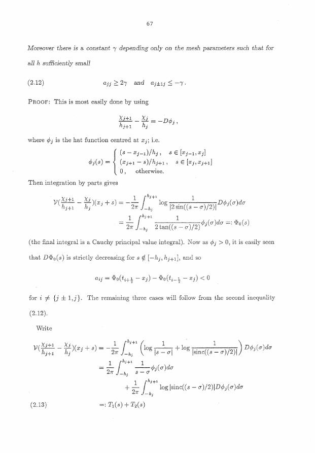
Moreover there is a constant 1 depending only on the mesh parameters such that for

all h sufficiently small

(2.12)

PROOF: This is most easily done by using

where r/J j is the hat function centred at Xj; i.e.

{ (s- Xj-r)/hi, s E [xj-1, Xj]

rPj(s) = (xj+l- .s)/hi+l, s E [xj,Xj+I]

0 , otherwise.

Then integration by parts gives

XHI Xi' 1 Jhj+l 1 V(-1 .-- -1 . J(Xj + 8) = --;;--- log 12 . (( '/ )IDr/Yj(CJ)dCJ

! y+l 1.1 ~Jr -h; sm 8 - CJ J 2 1

= _:!:_ ;·h; +1 1 -;-· (( )/ )c/Jj(CJ)dO" =: Wo(,s)

2;r -h; 2 tan s -- cr 2

(the final integral is a Cauchy principal value integral). Now as rPj > 0, it is easily seen

that DW0 (s) is strictly decreasing for s ~ [-hj,hi+l], and so

for i -=/- {j ± l,j}. The remaining three cases will follow from the second inequality

(2.12).

Write

(2.13)

68

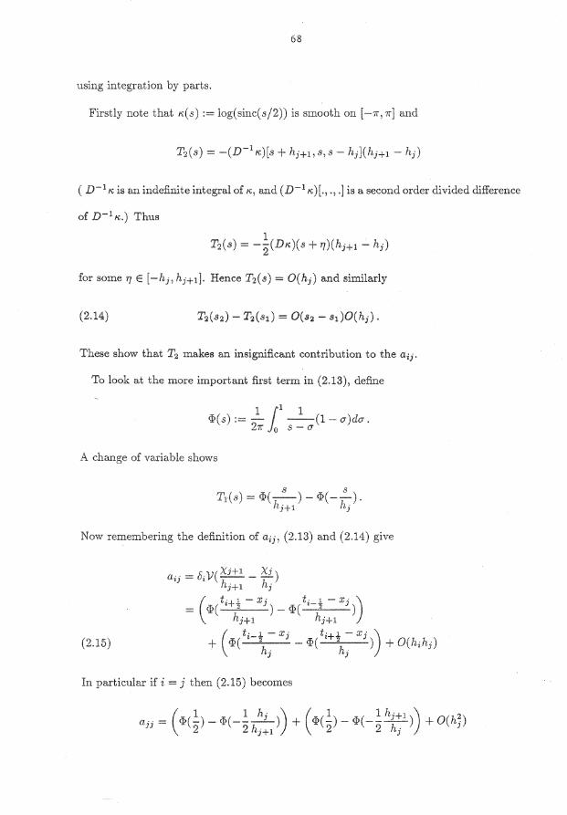
using integration by parts.

Firstly note that h:(s) := log(sinc(s/2)) is smooth on [-1r,1r] and

( n-1 h: is an indefinite integral of K, and (D- 1 ~~:)[., ., .] is a second order divided difference

of n- 1 ~i:.) Thus

for some 'f/ E [-hj,hj+l]· Hence Tz(s) = O(hj) and similarly

(2.14)

Tlwse show that Tz makes an insignificant contribution to the a;j.

To look at the more important first term in (2.13), define

1 11 1 (s) :=- --(1- a)da. 27r 0 s - (7

A change of variable shows

Tl( s) = ( -J s ) -(- hs ) . 1i+l ·j

Now remembering the definition of a;j, (2.13) and (2.14) give

(2.15)

In particular if i = j then (2.15) becomes

( 1 1 hj ) ( 1 1 hj+l \) 2 a··= 1>(-)-M---) + (-)-1>(---) +O(h·) JJ 2 \ 2 hj+l ' 2 2 hj J

69

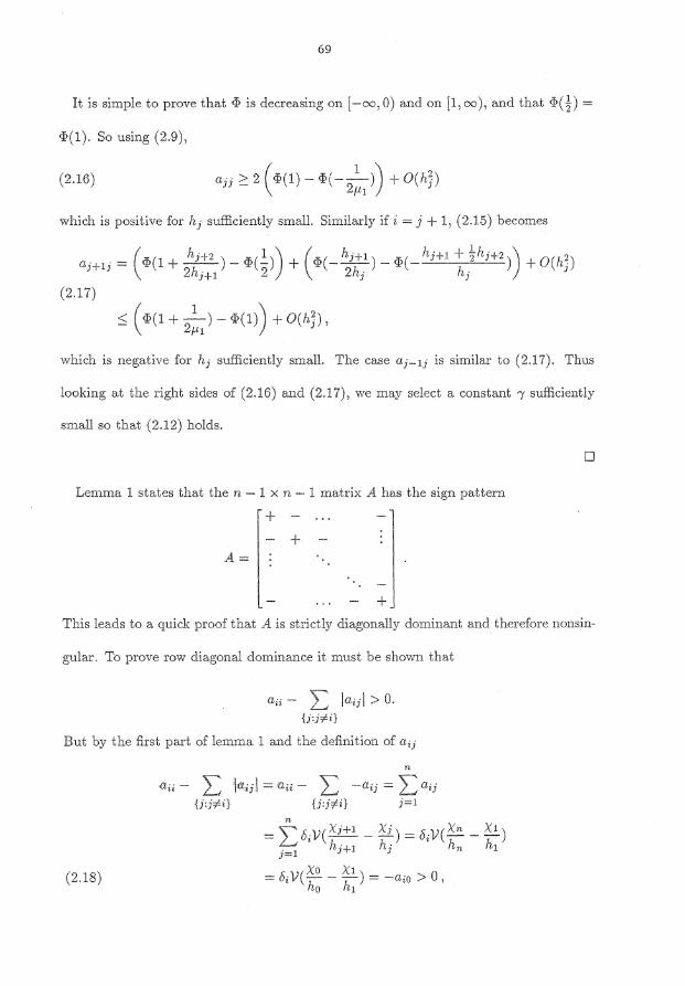
It is simple to prove that is decreasing on [ -oo, 0) and on [1, oo ), and that <[>a) =

<[>(1). So using (2.9),

(2.16)

which is positive for hj sufficiently small. Similarly if i = j + 1, (2.15) becomes

I 1 ' ::; I <l?(l + --)- <[>(1)) + O(h]),

\ 2f11

which is negative for hj sufficiently small. The case a.i-lj is similar to (2.17). Thus

looking a.t the right sides of (2.16) and (2.17), we may select a constant 1 sufficiently

small so that (2.12) holds.

D

Lemma 1 states that the n - 1 X n -· 1 matrix A has the sign pattern

·-l

+ This leads to a quick proof that A is strictly diagonally dominant and therefore nonsin-·

gular. To prove row diagonal dominance it must be shown that

a;;- 2::::: ja;jj > 0. {j:i;ti}

But by the first part of lemma 1 and the definition of a;j

" a;; - L •ja,rJ =a;; - ·2: -a;j = 2: a;1

{j:j#i} {j:j#i} j=l

= ~ 5;V(,:Yi+l - ~i) = o;V(Xn - Xl) Ld hj+l nj hn hl J=l

(2.18) Xo X1) = 5; V(-:- - -:;- = -a;o > 0 , ho n1

70

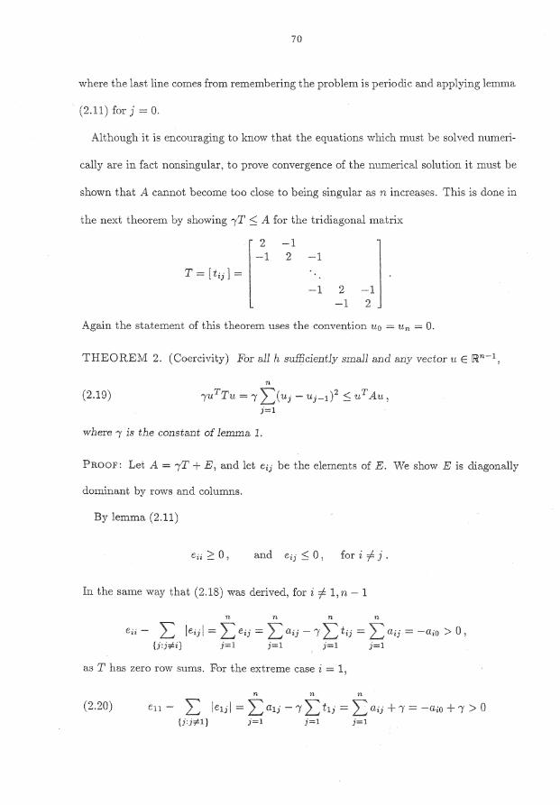
where the last line comes from remembering the problem is periodic and applying lemma

(2.11) for j = 0.

Although it is encouraging to know that the equations which must be solved numeri-

cally are in fact nonsingular, to prove convergence of the numerical solution it must be

shown that A cannot become too close to being singular as n increases. This is done in

the next theorem by showing 1T :::; A for the tridiagonal matrix

2 -1

J -1 2 -1

T = [t;i] =

-1 2

L -1 ') I ~ J

Again the statement of this theorem uses the convention u 0 = Un = 0.

THEOREM 2. (Coercivity) For all h sufficiently s.mall and any vector tt E lfiln-l,

(2.19) n

"(ttTTu = 7 2_)u.i- Uj_l) 2 :::; uT Au, j=l

where 1 is the constant of lemma 1.

PROOF: Let A= AfT+ E, and let e;j be the elements of E. We show E is diagonally

dominant by rows and columns.

By lemma (2.11)

eii >-: 0, and e;j :::; 0, for i f. j .

In the same way that (2.18) was derived, fori f. 1,n -1

n n n n

e;; - L je;j I = L e;j = L a;j - At L t;j = L a;j = -aio > 0 , {j:j,.;i} j=l j=l j=l j=l

as T has zero row sun1s. For the extreme case i = 1,

n n

(2.20) en - L le1j I = 2.:; ali - 7 L t1j = L a;j + 1 = -a;o + 7 > 0 {j:j'fl} j=l j=l j=l

71

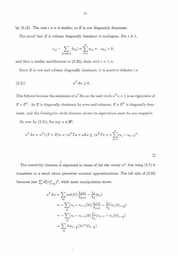
by (2.12). The case i = n is similar, so E is row diagonally dominant.

The proof that E is column diagonally dominant is analogous. For j !- 1,

n

ejj - L ieij I = L aij = --aoj > 0, {i:i;l!j} i=l

and then a similar modification to (2.20), deals with i = 1, n.

Since E is row and column diagonally dominant, it is positive definite; i.e.

(2.21)

This follows because the minimum of uT Eu on the unit circle uT u = 1 is an eigenvalue of

E + ET. As E is diagonally dominant by rows and columns, E + ET is diagonally dom-

inant, and the Gershgorin circle theorem shows its eigenvalues must be non-negative.

So now by (2.21 ), for any u E IR2 ,

n

UT Au= uT(rT + E)u = [UTTu + uEu;:::: ·yuTTu =I z)uj- Uj-1) 2 .

j=l

D

The coercivity theorem is expressed in terms of the the vector u", but using (2.7) it

translates to a result about piecewise constant approximations. The left side of (2.19)

becomes just I: ht ( v~_ 1 )'2, while some manipulation shows 2

ij

72

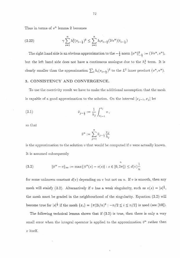
Thus in terms of v n lemma 2 becomes

(2.22) i=1 i=l

The right hand side is an obvious approximation to the -t norm jjvnjj:_.l. := (Vvn, vn), 2

but the left hand side does not have a continuous analogue due to the hr term. It is

clearly smaller than the approximation I:;i hi( vi-~ )2 to the L 2 inner product ( vn, vn).

3. CONSISTENCY AND CONVERGENCE.

To use the coercivity result we have to make the additional assumption that the mesh

is capable of a good approximation to the solution. On the interval [xj-l,xj]let

1 1Xj vi_~:=~. v,

) Xj -1

so that n

L X V-n ·- '' _]_ ··- . J-! h'

j=l J

is the approximation to the solution v that would be cornputed if v were actually known.

It is assumed subsequently

(3.2) llvn- vlloo := max{Jvn(s)- v(s)j: s E [0, 21r]}::; d(v)!_ . n

for some unknown constant d( v) depending on v but not on n. If v is smooth, then any

mesh will staisfy (3.2). Alternatively if v has a vveak singularity, such as v(s) = JsJ~,

the mesh must be graded in the neighbourhood of the singularity. Equation (3.2) will

become true for Jsl~ if the mesh {xi}= {r.(2i/n)2 : -n/2::; i:::; n/2} is used (see [10]).

The foilowing technical lemma shows that if (3.2) is true, then there is only a very

small error when the integral operator is applied to the approximation vn rather than

v itself.

73

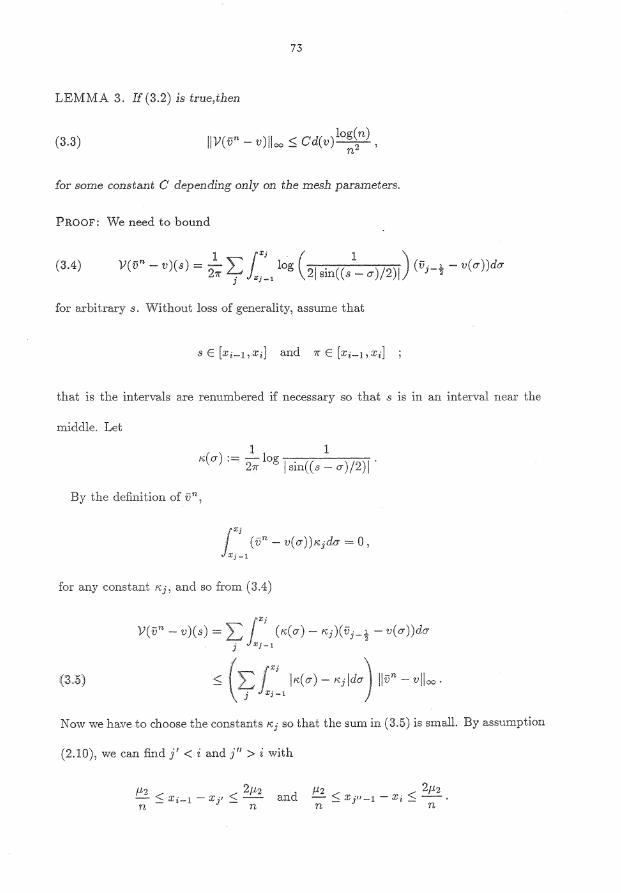
LEMMA 3. If (3.2) is true, then

(3.3) IIV(vn- v)lloo $ Cd(v)log~n), n

for some constant C depending only on the mesh parameters.

PROOF: We need to bound

(3.4) 1 1Xj ( 1 ) V(v"'- v)(s) =? ::S log\ 'JI . (( _ )/"')I. (vi-~- v(tY))diY

~1r j "'i-' ,~· s1n 8 0' ""'

for arbitrary 8. ·without loss of generality, assume that

sE[x;-l,x;] and 1rE[x;-1,xi]

that is the intervals are renmnbered if necessaJ·y so that s is in an interval near the

middle. Let

1 1 tc(cr) :=-log 1 . . )I.

271" 1 sm( ( s - O") /2. 1

By the definition of vn,

for any constant tc j, and so from

V(vn- v)(s) = 211~~, (tc(o-)- Kj)(vi-t- v(o-))dO"

::; ·(;c ri ~~~cO")- Kjldo-') llvn- vlloo · j J Xj -1

\'

Now we have to choose the constants Kj so that the sum in (3.5) is small. By assumption

(2.10), we can find j' i with

f.Lz 2f.Lz - $ Xi-1 - x j' $ - and n n

f.L2 2f.1.2 -$Xj"-l-x;$-. n n

74

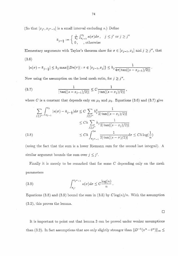
(So that [xj',Xj"-l] is a small interval excluding s.) Define

_ { ?; J:;_ 1 K(a)da, j ~ j' or j ?. j" K · 1 := J J

;-;; 0, , otherwise

Elementary arguments with Taylor's theorem show for a E [:c j-1! Xj] and j ?. j 11 , that

(3.6)

JK(a)- Rj_lJ ~ hjmax{JDK(r)J: T E [xj-I,Xj]} ~ hj 4 I (( 1 )/2)J' 2 1r,tan s-Xj-l

Now using the assumption on the local mesh ratio, for j ?. j 11 ,

(3.7) 1 c 1 I tan((s- Xj-1)/2)1 ~ I tan((s- Xj)/2)1'

where Cis a constant that depends only on {t1 and {!2 . Equations (3.6) and (3.7) give

j?:_j"

L 2 1 J,;(a)- R1·-1!da ~ C h1· I (( 'j· )I

• 2 2 tan s - J: · J 2 -1 j?:_j" . .1 '

< c h ~ h . -:----:--:--1-.,--:-.,.-, - ,~, 1 21 tan((s- Xj)/2)1

,;_]

(3.8) 12 11' 1 1 ~ Ch I (( )/ )Ida~ Chlog(-)

x;"- 1 2 tan s- cr 2 n

(using the fact that the sum is a lower Riemann sum for the second last integral). A

similar argument bounds the sum over j ~ j'.

Finally it is merely to be remarked that for some C depending only on the mesh

parameters

(3.9) t;"-' log(n) Jx K(a)dcr ~C--. xi' n

Equations (3.8) and (3.9) bound the sum in (3.5) by Clog(n)/n. With the assumption

(3.2), this proves the lemma..

0

It is important to point out that lemma 3 can be proved under weaker assumptions

than (3.2). In fact assumptions that are only slightly stronger than IID-1 ( vn- i!n)IJ oo ~

75

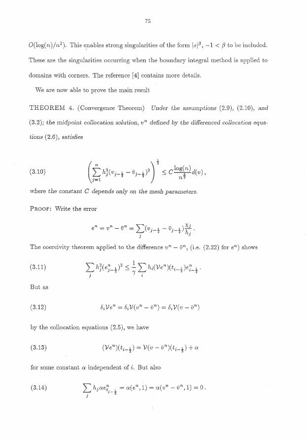
O(log( n) /n2 ). This 'Snables strong singularities of the form islj), -1 < (3 to be included.

These are the singularities occurring when the boundary integral method is applied to

domains with corners. The reference [4] contains more details.

IN'e are now able to prove the main result

THEOREM 4. (Convergence Theorem) Under the assumptions (2.9), (2.10), and

(3.2); the midpoint collocation solution, vn defined by the differenced collocation equa-

tions (2.6), satisfies

(3.10) ( n ) ~ 2 · \Z log(n) )'h.rv . .1.-ii- l.J · < C--d(v) ~ ]\ .J-2 ;-2 - §. '

j=l n2

where the constant C depends only on the mesh parameters.

PROOF: Write the error

n n -n ~( - )Xj e = v - v = L.. vj-~ - vj-~ T:.

j J

The coercivity theorem applied to the difference vn- vn, (i.e. (2.22) for en) shows

(3.11)

But as

(3.12)

by the collocation equations (2.5), we have

(3.13)

for some constant a independent of i. But also

(3.14)

76

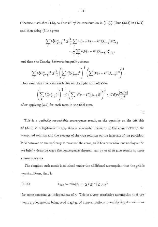
(Because v satisfies (1.5), so does vn by its construction in (3.1).) Thus (3.13) in (3.11)

and then using (3.14) gives

I:: h1( ej_~)2 :=:; ~ L h;( a+ V( v- vn)(t;_~))e?-~ J '

= ~ L h;V(v- vn)(t;_~)e?-~, '

and then the Cauchy-Schwartz inequality shows

.!. 1

1( hj('i-ll' ,; ~ ( 1( hj(ej-jl')' (~IV( v- v")(t,_l)l' r Then removing the common factor on the right and left sides

1

( ~ IV(v- vn)(t;_~w) 2 :::; Cd(v) 10~~n)

after applying (3.2) for each term in the final sum.

0

This is a perfectly respectable convergence result, as the quantity on the left side

of (3.10) is a legitimate norm, t.hat is a sensible measure of the error between the

computed solution and the average of the true solution on the intervals of the partition.

It is however an unusual way to measure the error, as it has no continuous analogue. So

we briefly describe ways the convergence theorem can be used to give results in more

common norms.

The simplest such result is obtained under the addi:tiona1 assumption that the grid is

quasi-uniform, that is

(3.15) hmin := min{hi: 1 :=:; i :=:; n} 2: /-i3/n

for some constant j-t3 independent of n. This is a very restrictive assumption that pre-

vents graded meshes being used to get good approximations to weakly singular solutions.

77

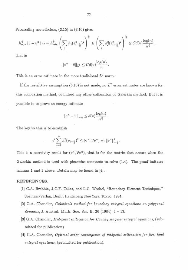
Proceeding nevertheless, (3.15) in (3.10) gives

' \! hi," llv - V" liP ~ h.!,,,. ( ~ h;( '7-t )') 00

that is

log(n) JJvn- vJJP:::; Cd(v)--'. n

This is an error estimate in the more traditional L 2 norm.

If the restrictive assumption (3.15) is not made, no L2 error estimates are known for

this collocation method, or indeed a..'ly other collocation or Galerkin method. But it is

possible to to prove an energy estimate

The key to this is to establish

n

-v' "\--., h2(v· )2 < (vn 1'vn) =· 1JvnJJ2 . I L._, 'l z-t - 'V I • t -"t" "

i=l

This is a coercivity result for ( vn, Vvn ), that is for the matrix that occurs when the

Galerkin method is used with piecewise constants to solve (1.4). The proof imitates

lemmas 1 and 2 above. Details may be found in [4].

REFERENCES.

[1] C.A. Brebbia, J.C.F. Telles, and L.C. Wrobel, "Boundary Element Teehniques,"

Springer-Verlag, Berlin Heidelberg NewYork Tokyo, 1984.

[2] G.A. Chandler, Galerkin's method for boundary integral equations on polygonal

domains, J. Austral. Math. Soc. Ser. B. 26 (1984), 1- 13.

[3] G.A. Chandler, Mid-point collocation for Cauchy singular integral equations, (sub

mitted for publication).

[4] G.A. Chandler, Optimal order convergence of midpoint collocation joT ji1·st kind

integral equations, (submitted for publication).

78

[5] N. Dyn and D. Levin, Iterative solution of systems originating from integral equa

tions and surface interpolation, SIAM J. Numer. Anal. 20 (1983), 377-390.

[6] F.R. de Hoog, "Product Integration Techniques for the Numerical Solution of

Integral Equations," Ph.D. thesis, Australian National University, Canberra, 1973.

[7] M.A. Jaswon, and G.T. Symm, "Integral Equations in Potential Theory and Elas

tostatics," Academic Press, London, 1977.

[8] G. Kuhn, Boundary element technique in elastostatics and linear fracture mechan

ic.s, in "Finite Element and Boundary Element Techniques from a Mathematical

and Engineering Point of View," (E. Stein and W.L. Wendland, Eds.), Springer

Verlag, Wien- New York, pp. 109 - 170.

[9] M.S. Longuet -Higgins and E.D. Cokelet, The deformation of steep surface waves

on water. I. A numerical method of computation, Proc. R. Soc. London A 350

(1976), 1 - 26.

[10] J .R. Rice, On the degree of convergence of nonlinear spline approximation, in

"Approximation with Special Emphasis on Spline Functions," (I.J. Schoenberg,

ed.), Academic Press, New York, 1969.

[11] E.P. Stephan, The h-p version of the Galerkin boundary element method for

integral equations on polygons and open arcs, in "Boundary Elements X," (C.A.

Brebbia, (Ed.)), Computational Mechanics, Southhampton, 1988, pp. 239- 245.

[12] W. Wendland, Strongly elliptic boundary integral equ.ations, in "The State of

the Art in Numerical Analysis," (A. Iserles, and M.J.D. Powell, Eds.), Clarendon,

Oxford, 1987, pp. 511 - 561.

Department of Mathematics,

The University of Queensland, Queensland 4072

Australia Email: [email protected]

OF BOUNDARY ELEMENT METHODS G.A. CHANDLER

Documents

Transcript of OF BOUNDARY ELEMENT METHODS G.A. CHANDLER