October 7-8, 2014 | NEPOOL MARKETS COMMITTEE

O C T O B E R 7 - 8 , 2 0 1 4 | N E P O O L M A R K E T S C O M M I T T E E

Matt BrewsterM A R K E T D E V E L O P M E N T

4 1 3 . 5 4 0 . 4 5 4 7 | M B R E W S T E R @ I S O - N E . C O M

ISO’s proposed zone sloped demand curves and overview of simulation model updatesfor evaluating zone curves

FCM Sloped Demand Curve:Capacity Zone demand curves

Topics

• Background slide 3

• Proposed zonal sloped demand curves– Overview of design slide 5– Key issues considered slide 6– Import-constrained capacity zones slide 8– Export-constrained capacity zones slide 11

• Simulation model updates slide 14

2

3

Background

• January 24th Order required ISO file a sloped demand curve by April 1st to implement for FCA9– Short time required deferring capacity zone demand curves– System-wide demand curve was approved on May 30th

• ISO is committed to developing capacity zone demand curves for FCA10 – May 30th Order encouraged ISO & NEPOOL to achieve this goal– Stakeholder discussions of zonal demand curves began on June 11th – ISO anticipates filing in mid-January, 2015

• Scope of the capacity zone demand curves project also includes conforming changes to the Forward Capacity Auction and removing the zonal administrative pricing rules

PROPOSED ZONAL DEMAND CURVESFor import- and export-constrained zones

Overview of proposed zonal demand curves

• Sloped demand curves for import- and export-constrained capacity zones for FCA10 and after– Replaces fixed demand constraints (LSR and MCL)– Fixed demand requirements have proven problematic

• Zonal curve cap-to-foot widths are proportional to system-wide demand curve (1x system ratio)

• No change to Net CONE values– Separate Net CONE for import zones if ≥115% of system Net CONE– Current estimates for CT, NEMA, and SEMA/RI are <105%

5

6

Key issues considered by the ISO

• ISO considered trade-offs among multiple factors to assess zonal alternatives, including interactions with the system demand curve– Simulations indicate a range of reasonable curves to address combination of reliability

and pricing objectives– Trade-offs exist because objectives are inter-related and curves that perform well on

one dimension will be poor on another (e.g., achieving low zonal price volatility raises zone purchases and costs)

• Import-constrained zones key considerations– Address upward price volatility (system curve helps address downward spikes)– Balance zonal and system reliability (affected by zone curve widths)– Cap quantity consistent with minimum requirements– Limit cost of purchasing considerably more than LSR

• Export-constrained zones key considerations– Address downward price volatility (system curve helps address upward spikes)– Prevent system reliability degradation of significantly exceeding MCL– Recognize cost benefits of abundant low-price supply

7

Key considerations (cont.)

• Balancing zonal and system reliability is one of the most evident trade-offs across the range of feasible zonal curves

• Primarily affected by width of zonal curves (cap and foot)– Due to changing the share of the total system demand which is

allocated to capacity zonesObjective Narrow Zone Curves Wide Zone Curves

Price volatility • Higher zone volatility• Lower system volatility

• Lower zone volatility• Higher system volatility

Reliability• Less likely to achieve zone minimum requirements• More likely to achieve NICR system-wide

• More likely to achieve zone minimum requirements• Less like to achieve NICR system-wide

Cost • Less zone excess• Lower costs

• More zone excess• Higher costs

8

Import-constrained zone sloped demand curves

• Cap– Price: MAX (1.6x Net CONE, CONE)– Quantity: MAX (TSA, LRA at 1-in-5)

• Foot– Price: $0/kW-month– Quantity: Cap x System cap-to-foot ratio

• Zone’s TTC not included in Cap or Foot– Simplifies definition and follows ISO-NE

convention for capacity requirements– Produces slightly narrower curves

• FCA7 System cap-to-foot ratio– CapSystem = 32,053 MW – FootSystem = 35,605 MW– Cap-to-Foot ratio = (35,605/32,053) = 111%

Note: FCA7 ICR values at http://www.iso-ne.com/static-assets/documents/markets/othrmkts_data/fcm/doc/summary_of_icr_values_expanded.xls

NEMA/Boston Zone Proposed Curve

Pric

e (%

of N

et C

ON

E)

MWNote: curve depicted based upon FCA7 ICR values

9

Import-constrained zone curves

Cap FootCurve Definition

Price 1.6x Net CONE $0

Quantity Max (TSA,LRA at 1-in-5 LOLE)

1x SystemCurve Ratio

Quantities based on FCA7Local ICAP (no TTC) 7,489 8,319

Slope Cap to FootChange in Price ($/kW-month) $17.7Change in Quantity (MW) 830

Slope ($/kW-month per 100 MW) $2.1



Quantity Max (TSA,LRA at 1-in-5 LOLE)

1x SystemCurve Ratio




Connecticut Zone Proposed Curve NEMA/Boston Zone Proposed Curve

MW MW

Notes: minimum demand curve cap price is 1x CONE; slopes based on Net CONE of $11.08; and foot set by System demand curve cap to ratio of 111% (based on FCA7)

Pric

e (%

of N

et C

ON

E)

Pric

e (%

of N

et C

ON

E)

10

Import-constrained zone simulation results

• Simulations demonstrate proposed curves can be expected to achieve balance of objectives for import zones

• Compared to current use of vertical demand within zones:– Some decrease in long-run price volatility– 20% (NEMA) and 25% (CT) reductions in the frequency below LSR– Increased excess above LSR (but by small fraction of zone LSR)

Quantity Zonal Load Cost

Average Standard Deviation

Frequency at Cap

Frequency of Price

Separation

Average Excess

(Deficit) Above LSR

Standard Deviation

Frequency Below

LSR

Frequency Below

TSA

Frequency Below 1-in-5

Average LOLE

Average Customer

Costs

Average of Bottom

20%

Average of Top 20%

($/kW-m) ($/kW-m) (% of draws) (% of draws) (MW) (MW) (% of draws) (% of draws) (% of draws) (events/yr) ($mil/year) ($mil/year) ($mil/year)

NEMA/Boston1.0x No TTC (ISO-NE Proposal) $12.2 $4.1 18.9% 16.9% 743 405 13.7% 13.7% 10.2% 0.109 $946 $497 $1,421Vertical in Import Zones $12.2 $4.1 21.1% 16.9% 633 405 17.1% 17.1% 10.1% 0.107 $947 $509 $1,418

Connecticut1.0x No TTC (ISO-NE Proposal) $12.2 $3.9 15.9% 21.9% 429 469 14.1% 10.9% 13.3% 0.120 $1,221 $696 $1,739Vertical in Import Zones $12.2 $4.2 22.6% 18.9% 307 470 18.9% 14.3% 13.7% 0.123 $1,222 $679 $1,777

Price

Note: both runs presented above apply the ISO-NE proposed 1x system ratio curve in Maine and the approved System-wide sloped demand curve.

11

Export-constrained zone sloped demand curves

Maine Export Zone Proposed Curve• Cap– Price: MAX (1.6x Net CONE, CONE)– Quantity: MCL x System cap-to-NICR ratio

• Foot– Price: $0/kW-month– Quantity: MCL x System cap-to-foot ratio

• Curve is oriented around the probabilistic MCLrequirement in same manner as System curve

• FCA7 System demand curve ratios– NICR = 32,968 MW– CapSystem = 32,053 MW – FootSystem = 35,605 MW– Cap-to-NICR ratio = (32,053/32,968) = 97%– Cap-to-foot ratio = (35,605/32,053) = 111%

Note: FCA7 ICR values at http://www.iso-ne.com/static-assets/documents/markets/othrmkts_data/fcm/doc/summary_of_icr_values_expanded.xls

Export zone cap-to-foot ratio is the same as the System-wide curve cap-to-foot ratioPr

ice

(% o

f Net

CO

NE)

MWNote: curve depicted based upon FCA7 ICR values

12

Maine export-constrained zone curve and simulation results

Quantity Zonal Load CostAverage Standard

DeviationFrequency

at CapFrequency

of Price Separation

Average Quantity

Above (Below) MCL

Standard Deviation

SystemLOLE

Unconstrained System

LOLE

Final Customer

Costs

Averageof Bottom

20%

Averageof Top 20%

($/kW-m) ($/kW-m) (% of draws) (% of draws) (MW) (MW) (events/yr) (events/yr) ($mil/year) ($mil/year) ($mil/year)

1x System Ratio (ISO-NE Proposal) $10.0 $4.1 4.0% 19.1% (267) 168 0.120 0.109 $287 $120 $457Vertical $10.0 $4.5 4.9% 13.7% (385) 168 0.118 0.106 $287 $99 $460

Price

Note: both runs presented above apply the ISO’s proposed 1x curve in import-constrained zones and the approved System-wide sloped demand curve.

• Simulations demonstrate proposed curve can be expected to achieve balance of objectives for export zones

• Compared to current use of MCL

• Reduced zone price volatility

• Clear more capacity in export zone (still below MCL on average)

• Slight increase in System LOLE



Quantity MCL x System cap-to-NICR ratio

MCL x System NICR-to-foot ratio




Maine Export Zone Proposed Curve

Notes: minimum demand curve cap price is 1x CONE; slopes based on Net CONE of $11.08; cap and foot set by System demand curve ratios of 97% and 108%, respectively (based on FCA7)

13

System-wide simulation results

• Proposed capacity zone demand curves appear to strike a good balance between zonal and system objectives

• Simulation results demonstrate trade-offs among objectives– System price volatility and reliability indices worsen somewhat when

modeling zonal demand curves– Wider zonal curves would exaggerate these outcomes, narrow curves

would have lesser impact (Brattle materials demonstrate a range)

Reliability System Load Cost

AverageStandard Deviation

Frequency at Cap

System Average

LOLE

Unconstra ined Average LOLE

Average Reserve Margin

Reserve Margin St. Dev.

Frequency Below NICR

Frequency Below

1-in-5 in RoP

AverageAverage of

Bottom 20%

Average ofTop20%

($/kW-m) ($/kW-m) (% of draws) (events/yr) (events/yr) (%) (%) (% of draws) (% of draws) ($mil/yr) ($mil/yr) ($mil/yr)

System-Wide Demand Curve and ISO Proposed Zonal Sloped Demand Curves

$11.1 $3.8 6.3% 0.120 0.109 12.9% 2.7% 37.2% 10.1% $4,506 $2,685 $6,428

System-Wide Demand Curve and All Vertical Zonal Demand

$11.1 $3.6 4.7% 0.120 0.104 13.1% 2.7% 35.6% 8.9% $4,513 $2,669 $6,378

Price

Note: both runs presented above apply the approved System-wide sloped demand curve; the “All Vertical” case applies fixed LSR and MCL demand for capacity zones

SIMULATION MODEL UPDATESOverview of simulation model updates for evaluating capacity zone sloped demand curves

15

Overview of simulation model updates for evaluating capacity zone sloped demand curves

• Two related aspects of the simulation model were updated to reflect ISO’s auction clearing rules and LOLE metrics 1) Cleared supply with import-constrained zone price separation2) Calculation of an additional system-wide LOLE metric

• Changes were identified during the ISO’s detailed assessment of the candidate zonal demand curves

• Updated simulation results show small changes consistent with expectations of adjusted model– Updated results are described in October MC material from Brattle

• Simulations use modified model beginning with October MC

16

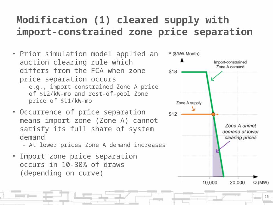
Modification (1) cleared supply with import-constrained zone price separation

• Prior simulation model applied an auction clearing rule which differs from the FCA when zone price separation occurs– e.g., import-constrained Zone A price of

$12/kW-mo and rest-of-pool Zone price of $11/kW-mo

• Occurrence of price separation means import zone (Zone A) cannot satisfy its full share of system demand– At lower prices Zone A demand increases

• Import zone price separation occurs in 10-30% of draws (depending on curve)

17

Modification (1) explanation continued

• Prior simulation model had assumed the FCA would purchase additional supply outside Zone A to satisfy the unmet portion of system-wide demand not met within Zone A

• However, FCA will not clear this additional supply because:– Import zone demand is a share of the system demand that must be

met within the zone (consistent with ICR studies)– Additional supply outside Zone A cannot satisfy Zone A requirement– Purchasing required Zone A capacity in reconfiguration auctions could

lead to excess procurement for the system

• Auction outcome for import-constrained zones are identical with prior and revised model regardless of price separation; and identical in all zones when no price separation occurs

18

Modification (1) illustrations of FCA outcome

• The four examples that follow demonstrate the FCA clearing when import-constrained zone price separation occurs

• Each demonstrates the same mechanics under different configurations of import zone and system demand– Example 1: Zone and System vertical demand (FCA8 and prior)– Example 2: Zone vertical and System sloped demand (FCA9)– Examples 3 & 4: Zone and System sloped demand (FCA10 and beyond)

• All examples include two capacity zones for simplicity– Import-constrained Zone A– Rest-of-Pool Zone B

19

Modification (1)

Example 1: Zone and System vertical demand

• FCA8 and prior

• Import Zone A, Rest-of-Pool (ROP) Zone B

• The Zone A unmet demand quantity (red) is constant at lower prices

• FCA does not purchase Zone A unmet demand from ROP resources

• Extra ROP supply cannot serve Zone A capacity requirement

ROP Cleared Supply

Zone ACleared Supply

20

Modification (1)

Example 2: Zone vertical and System sloped

• FCA9

• Import Zone A, ROP Zone B

• Same observations as example 1

• Sum of Zone A and ROP cleared MW plus Zone A unmet demand (red) correspond to system-wide demand curve price applicable in ROP

ROP Cleared Supply


21

Modification (1)

Example 3: Zone and System sloped demand

• FCA10 and beyond


• Same observations as examples 1 and 2, except Zone A demand now is price-dependent (sloped curve)

• The amount of Zone A unmet demand (red) depends on the ROP clearing price

• If Zone A and ROP have the same clearing price, there is no Zone A unmet demand

ROP Cleared Supply


22

Modification (1)

Example 4: Zone and System sloped demand, using long-run average clearing prices

• FCA10 and beyond


• Same observations as examples 1, 2, and 3

• Example with Zone A and ROP prices at simulation long-run average values ($12.2/kW-mo and $11.1/kW-mo, respectively)

• With ISO proposed curves, unmet import zone demand is <50MW per zone at long-run average prices

ROP Cleared Supply


Modification (2) calculation of system-wide LOLE metrics

• Metric previously labeled as “system LOLE” is more accurately described as an unconstrained system LOLE– Reflects LOLE absent import-constrained zones similar to the modeling

of Net ICR without transmission constraints

• NPCC reliability criteria incorporate subarea LOLE in the determination of system LOLE– If import zone capacity is below LRA requirement, the zone’s LOLE is

worse than 1-in-10 and will be the dominant factor in system LOLE– The zone is the “weakest link” in the system

• For example: with a capacity zone at 1-in-5 (0.200) LOLE the system will be close to 1-in-5 LOLE regardless of whether supply is adequate to meet all other requirements

23

24

Modification (2) explanation continued

• Metric previously labeled as “system LOLE” will now be labeled “Unconstrained System LOLE”– Measure of system LOLE based on total supply relative to Net ICR*

• New “Constrained System LOLE” metric reflects NPCC method– Measure of system LOLE with transmission constraints– Demonstrates whether all zones have met their requirement

• Import zone LOLE calculation was modified slightly to be consistent with system LOLE change

• Unconstrained System LOLE provides additional information for comparing the candidate zonal demand curves– Shows effect of inter-zonal price separation events (driven primarily by

zone demand curve shape) on achieving Net ICR*Brattle adjusts the “Unconstrained System LOLE” to reflect lower reliability of export-constrained zone capacity above MCL

25

Recap of simulation model updates

• Modification (1) for import zone price separation– FCA treats unmet demand equivalently with vertical or sloped demand– Absent price separation there is no unmet demand (70-90% of draws)

• Modification (2) for system-wide LOLE metrics– NPCC reliability criteria requires accounting for “weakest link”– New “Constrained System LOLE” reflects NPCC guidelines

• The modeling changes represent closely related concepts– FCA won’t clear extra supply outside zone to cover unmet demand– Extra supply outside zone has very limited impact on achieving zone or

system minimum reliability criteria

• Revised simulation model applied for analysis of zonal sloped demand curves beginning with October MC materials

SUMMARY AND SCHEDULERecap and next steps

27

Summary and schedule

• Summary– There are a range of reasonable zonal curves based on Brattle analysis– ISO proposed zonal curves reflect balance of reliability and pricing

objectives at zonal and system level – ISO requested two modifications to the Brattle simulation model for

the analysis of capacity zone demand curves

• Schedule– November – additional discussion (design and tariff) – December – MC vote– January 2015 – filing with FERC

October 7-8, 2014 | NEPOOL MARKETS COMMITTEE

Documents

Transcript of October 7-8, 2014 | NEPOOL MARKETS COMMITTEE