Occlusion in Acoustic Tracking - Computer Science · Approach to Occlusion in Acoustic Tracking....
112
WHISPER: A Spread Spectrum Approach to Occlusion in Acoustic Tracking by Nicholas Michael Vallidis A dissertation submitted to the faculty of The University of North Carolina at Chapel Hill in partial fulfillment of the requirements for the degree of Doctor of Philosophy in the Department of Computer Science. Chapel Hill 2002
Transcript of Occlusion in Acoustic Tracking - Computer Science · Approach to Occlusion in Acoustic Tracking....

WHISPER: A Spread Spectrum Approach to
Occlusion in Acoustic Tracking
byNicholas Michael Vallidis
A dissertation submitted to the faculty of The University of North Carolina at ChapelHill in partial fulfillment of the requirements for the degree of Doctor of Philosophyin the Department of Computer Science.
Chapel Hill2002

ii
Copyright c© 2002
Nicholas Michael Vallidis
All rights reserved

iii
ABSTRACT
NICHOLAS MICHAEL VALLIDIS. WHISPER: A Spread SpectrumApproach to Occlusion in Acoustic Tracking.
(Under the direction of Gary Bishop.)
Tracking systems determine the position and/or orientation of a target object,
and are used for many different purposes in various fields of work. My focus is
tracking systems in virtual environments. While the primary use of tracking for
virtual environments is to track the head position and orientation to set viewing
parameters, another use is body tracking—the determination of the positions of the
hands and feet of a user. The latter use is the goal for Whisper.
The largest problem faced by body-tracking systems is emitter/sensor occlusion.
The great range of motion that human beings are capable of makes it nearly impossible
to place emitter/sensor pairs such that there is always a clear line of sight between
the two. Existing systems either ignore this issue, use an algorithmic approach to
compensate (e.g., using motion prediction and kinematic constraints to “ride out”
occlusions), or use a technology that does not suffer from occlusion problems (e.g.,
magnetic or mechanical tracking devices). Whisper uses the final approach.
In this dissertation I present Whisper as a solution to the body-tracking prob-
lem. Whisper is an acoustic tracking system that uses a wide bandwidth signal to
take advantage of low frequency sound’s ability to diffract around objects. Previous
acoustic systems suffered from low update rates and were not very robust of envi-
ronmental noise. I apply spread spectrum concepts to acoustic tracking in order to
overcome these problems and allow simultaneous tracking of multiple targets using
Code Division Multiple Access.

iv
The fundamental approach is to recursively track the correlation between a trans-
mitted and received version of a pseudo-random wide-band acoustic signal. The offset
of the maximum correlation value corresponds to the delay, which corresponds to the
distance between the microphone and speaker. Correlation is computationally expen-
sive, but Whisper reduces the computation necessary by restricting the delay search
space using a Kalman filter to predict the current delay of the incoming pseudo-noise
sequence. Further reductions in computation expense are accomplished by reusing
results from previous iterations of the algorithm.

v
To my parents for teaching me the value of education
and
To my wife Amy for being the most incredible woman in the world

vi
Acknowledgments
Thanks to
• Gary Bishop for being my advisor and providing the original idea for Whisper.Whenever I use “we” or “our” in this dissertation, it refers to my collaborationwith Gary Bishop.
• My committee members for their time and insight: Gary Bishop, Greg Welch,Leandra Vicci, Henry Fuchs and John Poulton
• Collaborators that have made innumerable contributions to this work: ScottCooper, Jason Stewart, John Thomas, Stephen Brumback and Kurtis Keller
• Scott Cooper for the Whisper concept drawing (Figure 6.1)
• My family for teaching me to be curious about the world around me and fortolerating my tendency to disassemble anything I could get my hands on.
• My wife for being so understanding about the life of a graduate student. I willhappily support her in whatever she decides to pursue for the rest of our lives.
I also greatly appreciate the following groups/programs for the funding provided tothis work:
• NASA Graduate Student Researcher Program
• UNC-CH Department of Computer Science Alumni Fellowship
• Office of Naval Research contract no. N00014-01-1-0064

vii
Contents
Acknowledgments vi
List of Tables x
List of Figures xi
1 Introduction 1
1.1 Motivation . . . . . . . . . . . . . . . . . . . . . . . . . . . . . . . . . 1
1.2 A Solution . . . . . . . . . . . . . . . . . . . . . . . . . . . . . . . . . 2
1.3 Thesis Statement . . . . . . . . . . . . . . . . . . . . . . . . . . . . . 3
1.4 Summary of Results . . . . . . . . . . . . . . . . . . . . . . . . . . . 3
1.5 Overview . . . . . . . . . . . . . . . . . . . . . . . . . . . . . . . . . . 4
2 Related Work 6
2.1 Tracking Categories . . . . . . . . . . . . . . . . . . . . . . . . . . . . 7
2.1.1 Mechanical . . . . . . . . . . . . . . . . . . . . . . . . . . . . 7
2.1.2 Acoustic . . . . . . . . . . . . . . . . . . . . . . . . . . . . . . 8
2.1.3 Electromagnetic (Optical and Radio Frequency) . . . . . . . . 8
2.1.4 Magnetic . . . . . . . . . . . . . . . . . . . . . . . . . . . . . . 9
2.1.5 Inertial . . . . . . . . . . . . . . . . . . . . . . . . . . . . . . . 9
2.2 Acoustic Tracking Systems . . . . . . . . . . . . . . . . . . . . . . . . 10
2.3 Spread Spectrum Tracking Systems . . . . . . . . . . . . . . . . . . . 13

viii
2.4 Body-centered Tracking Systems . . . . . . . . . . . . . . . . . . . . . 15
3 Spreading and Shaping the Spectrum 17
3.1 General Communications Principles . . . . . . . . . . . . . . . . . . . 17
3.2 What Does Spread Spectrum Mean? . . . . . . . . . . . . . . . . . . 19
3.3 Classification of Spread Spectrum Schemes . . . . . . . . . . . . . . . 20
3.4 A Closer Look at Direct Sequence CDMA . . . . . . . . . . . . . . . 20
3.4.1 Pseudonoise codes . . . . . . . . . . . . . . . . . . . . . . . . 21
3.4.2 Acquiring and decoding a DS signal . . . . . . . . . . . . . . . 23
3.5 Wide Bandwidth Signals in Acoustic Tracking . . . . . . . . . . . . . 25
3.5.1 Low Frequencies Allow Diffraction . . . . . . . . . . . . . . . . 26
3.5.2 High Frequencies Yield Precision . . . . . . . . . . . . . . . . 28
3.6 Spectrum Shaping . . . . . . . . . . . . . . . . . . . . . . . . . . . . 29
4 Range Measurement and Occlusion 31
4.1 System Configuration . . . . . . . . . . . . . . . . . . . . . . . . . . . 31
4.2 Algorithm . . . . . . . . . . . . . . . . . . . . . . . . . . . . . . . . . 32
4.2.1 Description . . . . . . . . . . . . . . . . . . . . . . . . . . . . 34
4.2.2 Selecting Parameters . . . . . . . . . . . . . . . . . . . . . . . 44
4.3 Dealing With Occlusion . . . . . . . . . . . . . . . . . . . . . . . . . 51
4.3.1 Effect of Occlusion on Signal . . . . . . . . . . . . . . . . . . . 52
4.3.2 Effect of Occlusion on Correlation . . . . . . . . . . . . . . . . 54
4.3.3 Effect of Occlusion on WHISPER . . . . . . . . . . . . . . . . 56
5 Three-Dimensional Tracking and Multiple Targets 60
5.1 Calculating 3D Position . . . . . . . . . . . . . . . . . . . . . . . . . 60
5.1.1 Modifications to the Kalman Filter . . . . . . . . . . . . . . . 62
5.1.2 Error from Nonlinearity . . . . . . . . . . . . . . . . . . . . . 65

ix
5.2 Performance . . . . . . . . . . . . . . . . . . . . . . . . . . . . . . . . 66
5.2.1 Factors Affecting Performance . . . . . . . . . . . . . . . . . . 67
5.2.2 Relationship Between 1D and 3D Performance . . . . . . . . . 75
5.2.3 Static performance . . . . . . . . . . . . . . . . . . . . . . . . 78
5.2.4 Dynamic Performance . . . . . . . . . . . . . . . . . . . . . . 78
5.2.5 Latency . . . . . . . . . . . . . . . . . . . . . . . . . . . . . . 81
5.3 Tracking multiple targets . . . . . . . . . . . . . . . . . . . . . . . . . 83
5.3.1 Microphones Fixed or on Targets? . . . . . . . . . . . . . . . . 84
5.3.2 Selecting the Codes . . . . . . . . . . . . . . . . . . . . . . . . 86
5.3.3 Limits on Number of Targets . . . . . . . . . . . . . . . . . . 88
6 Conclusions and Future Work 89
6.1 Summary of results . . . . . . . . . . . . . . . . . . . . . . . . . . . . 89
6.2 Other Applications . . . . . . . . . . . . . . . . . . . . . . . . . . . . 90
6.3 Future Work . . . . . . . . . . . . . . . . . . . . . . . . . . . . . . . . 91
6.3.1 Adaptations . . . . . . . . . . . . . . . . . . . . . . . . . . . . 91
6.3.2 Modifications . . . . . . . . . . . . . . . . . . . . . . . . . . . 93
References 96

x
List of Tables
4.1 Comparison of measured and theoretical diffracted path lengths . . . 57
4.2 Maximum error in diffracted path length measurement . . . . . . . . 59
5.1 Mean position for static target locations . . . . . . . . . . . . . . . . 79
5.2 Comparison of measured and Whisper-estimated distances . . . . . 79
5.3 Latency of Whisper algorithm . . . . . . . . . . . . . . . . . . . . . 83
5.4 Comparison of Matlab random and maximal length sequences . . . . 88

xi
List of Figures
2.1 Signals used by acoustic tracking devices . . . . . . . . . . . . . . . . 11
3.1 Maximal length sequences . . . . . . . . . . . . . . . . . . . . . . . . 22
3.2 Multi-path interference identification in direct sequence systems . . . 26
3.3 Surface diffraction physics . . . . . . . . . . . . . . . . . . . . . . . . 27
3.4 Using diffraction in acoustic tracking . . . . . . . . . . . . . . . . . . 28
3.5 High frequencies provide accuracy . . . . . . . . . . . . . . . . . . . . 29
3.6 Effect of filtering pseudonoise signal on correlation function . . . . . . 30
4.1 System diagram . . . . . . . . . . . . . . . . . . . . . . . . . . . . . . 32
4.2 Whisper algorithm . . . . . . . . . . . . . . . . . . . . . . . . . . . 34
4.3 Pseudocode for initialization and Kalman filter. . . . . . . . . . . . . 35
4.4 Example correlation result and its peaks . . . . . . . . . . . . . . . . 39
4.5 Quadratic functions fit to correlation peaks . . . . . . . . . . . . . . . 39
4.6 Pseudocode for computation reuse. . . . . . . . . . . . . . . . . . . . 40
4.7 Illustration of computation reuse algorithm . . . . . . . . . . . . . . . 41
4.8 Shape of pseudonoise autocorrelation . . . . . . . . . . . . . . . . . . 43
4.9 Comparison of quadratic and triangular correlation peak fitting . . . 44
4.10 Range measurement variance . . . . . . . . . . . . . . . . . . . . . . . 50
4.11 Frequency response of creeping wave attenuation . . . . . . . . . . . . 53
4.12 Spectrogram of occluded signal . . . . . . . . . . . . . . . . . . . . . 53
4.13 Effect of occlusions on correlation peak . . . . . . . . . . . . . . . . . 56
4.14 Explanation of parameters for calculating the diffracted path length . 59
5.1 Whisper’s microphone array . . . . . . . . . . . . . . . . . . . . . . 66

xii
5.2 Error introduced by quadratic estimate . . . . . . . . . . . . . . . . . 71
5.3 Speaker radiation pattern . . . . . . . . . . . . . . . . . . . . . . . . 72
5.4 Whisper’s original speakers . . . . . . . . . . . . . . . . . . . . . . . 73
5.5 Effect of GDOP . . . . . . . . . . . . . . . . . . . . . . . . . . . . . . 76
5.6 Whisper dynamic performance . . . . . . . . . . . . . . . . . . . . . 80
5.7 Target velocity during dynamic performance run . . . . . . . . . . . . 81
6.1 Conceptual drawing of a body-centered Whisper system . . . . . . . 93
Chapter 1
Introduction
1.1 Motivation
Tracking systems determine the position and/or orientation of a target object, and
are used for many different purposes in various fields of work. Air-traffic controllers
use radar tracking systems to monitor the current positions of airplanes. Surveyors
use the Global Positioning System (GPS) to measure distances and define boundaries.
Virtual environments use tracking systems as a means of monitoring the position and
orientation of the user’s head. They even serve as generic human-computer interface
devices as with the computer mouse.
My focus is tracking systems in virtual environments. While the primary use is
to track head position and orientation to set viewing parameters such that images
rendered to a head-mounted display look correct and move appropriately, another
use in virtual environments is body tracking—the determination of the positions of
the hands and feet of a user, as well as nearby objects in some cases. This allows
the computer to draw an avatar of the user in the virtual environment. Also, the
user can then interact with the environment in a natural way, or by using gestures as
suggested by [Mine 97]. This second use of tracking systems for virtual environments
(tracking hands and feet) is the goal for Whisper.

2
The largest problem faced by body-tracking systems is the issue of occlusion. The
great range of motion that human beings are capable of make it nearly impossible to
place emitter/sensor pairs such that there is always a clear line of sight between the
two. Past systems either ignored this issue or used magnetic or mechanical tracking
devices. Ignoring the issue is troublesome because it means that there are situations
when the tracking device will not work (e.g., optical and ultrasonic systems). Mag-
netic devices have their own problems including large infrastructure and/or power
requirements making them unsuitable for mobile use, susceptibility to interference
from metal and/or ferrous objects, and high latency (mostly due to the large amount
of filtering necessary to provide good measurements). Mechanical devices have their
own troubles coming from limits on the number of tracked targets or the complexity
of donning and doffing the mechanical system.
1.2 A Solution
In this dissertation I present Whisper as an approach to the body-tracking prob-
lem. Whisper is an acoustic tracking system that uses a wide bandwidth signal in or-
der to take advantage of low frequency sound for its ability to diffract around objects.
As Section 4.3 describes, low frequency sound diffracts further (than ultrasound) into
the shadow zone behind an occluding object, allowing Whisper to continue tracking
during most occlusion events that might happen with a body-tracking system.
Previous acoustic systems suffered from low update rates and were not very toler-
ant of noise in the environment (both external and multipath interference). Chapter 3
presents the basic concepts of spread spectrum communications and how they over-
come these difficulties. I apply spread spectrum concepts to acoustic tracking in order
to overcome these problems and allow simultaneous tracking of multiple targets using
Code Division Multiple Access (CDMA).

3
The Whisper algorithm centers on the autocorrelation shape of a noise sequence.
The autocorrelation of an infinite random sequence is a delta function. The correlation
of a finite random sequence and a delayed copy of itself has a large enough correlation
peak that it allows measurement of the delay between the two signals. By playing a
random sequence through a speaker and receiving it through a microphone, correlation
can be used to determine the delay between the two sequences. This delay is due
to the propagation time of the signal through the air between the speaker and the
microphone.
Traditional correlation is computationally expensive. However, Whisper reduces
the computation necessary by restricting the delay search space using a Kalman filter
to predict the current delay of the incoming noise sequence. Further improvements
in computation expense are made by reusing results from previous iterations of the
Whisper algorithm.
1.3 Thesis Statement
Spread spectrum technology applied to acoustic tracking produces a robust tracking
device with better performance than existing acoustic systems. Extending the frequency
range of the signal down into the audible range enables tracking in the presence of
occlusions.
1.4 Summary of Results
Whisper calculates 1000 3D positions for two targets per second. Simulations
show that Whisper does this with a maximum latency of 18-49 milliseconds, depend-
ing on the signal to noise ratio and range to the target. In un-occluded situations,
experiments with a static target demonstrate the 3D position estimates have a small

4
standard deviation (0.46 to 0.91 mm depending on transducer geometry and signal to
noise ratio). These static measurements cover a cubic volume approximately 35 cm on
a side located approximately 20 cm from the plane containing the array of three mi-
crophones . Increasing the baseline distances between the microphones would increase
the volume over which Whisper can attain low variance estimates.
Experiments with two targets mounted rigidly to one another result in a standard
deviation of only 2.0 mm on the distance between the estimated positions of the two
targets even though the targets travelled at velocities up to 3 meters per second.
In occluded situations, range measurements increase by an amount predictable with
knowledge of the geometry of the occluder. Whisper currently does not recognize
the presence of occlusions and so the increased range measurements introduce error
into the target’s position estimate. Occluding all three range measurements results
in the largest error, while occluding only one measurement results in a smaller error.
Whisper is currently implemented as a bench-top prototype, but its abilities
show that it should be well-suited for use in a body-centered system. The amount
of computation required by Whisper’s algorithm is small enough that it could be
easily implementable in an off-the-shelf digital signal processor (DSP) making for a
small, light tracking device that could be mounted to the user.
1.5 Overview
Chapter 2 discusses previous work in tracking systems for virtual environments
including acoustic, spread spectrum and body-centered systems. Chapter 3 presents
an overview of spread spectrum communications for those unfamiliar with the topic as
well as the advantages of using the wide bandwidth acoustic signal that results from
the application of these techniques. Chapter 4 describes the one-dimensional version
of Whisper along with the plausibility of using diffraction to overcome occlusion.
5
Chapter 5 presents a three-dimensional Whisper system capable of simultaneously
tracking two targets and describes its performance and considerations in expanding
beyond two targets. Chapter 6 summarizes the results of this work and provides
opportunities for future contributions involving Whisper.

Chapter 2
Related Work
A tracking system determines the position and/or orientation of a target object.
Computer mice are tracking systems that most readers have used. A mouse tracks
the two-dimensional position of a user’s hand as it moves over the surface of a desk.
Most modern mice use a mechanical or optical system to perform this task, although
there has been at least one commercial ultrasonic mouse.
In order to render the appropriate images to show to a user wearing a head-
mounted display, the rendering engine must know the position and orientation of the
user’s head. This tracking problem has occupied researchers in the area of virtual
environments for over thirty years now. Recently, systems such as the UNC HiBall
[Welch 01] and Intersense’s Constellation [Foxlin 98b] have provided robust and ex-
tremely accurate solutions to this problem. However, there is still an unmet need for
systems to track the user’s limbs in order to draw a proper avatar or allow natural
interfaces with the virtual environment [Mine 97].
This chapter begins by discussing the five basic categories of tracking devices for
virtual environments. Then it continues into a more thorough discussion of acoustic
tracking systems. With this background, the last sections focus on two specific types
of tracking systems: spread spectrum and body-centered.

7
2.1 Tracking Categories
All current tracking systems belong to one of five categories depending on the
method they use to make their measurements. These are mechanical, acoustic, elec-
tromagnetic, magnetic and inertial. Each category has advantages and disadvantages
that suit a specific environment or a specific purpose. There have been many liter-
ature reviews describing the various options along with their benefits, so they will
not be repeated here. Instead, this section contains a brief description of the five
categories. Suggested references for further information are [Meyer 92], [Ferrin 91]
and [Bhatnagar 93].
2.1.1 Mechanical
Mechanical systems are the simplest to understand as their workings are often
visible [Meta Motion 00, Measurand Inc. 00]. They are usually constructed as a me-
chanical arm with one end fixed and the other attached to the tracking target. The
mechanical arm has joints that allow the target to move around. Each joint is in-
strumented, typically by a potentiometer or optical encoder, to determine its current
state. A series of matrices containing a mathematical description of the arm trans-
forms the joint states into the position of the target.
Mechanical arms add weight and resistance to the motion of a target. This tends to
change the dynamics of target motion or, more significantly in virtual environments,
tire a user who must pull the arm around. Further, multiple mechanical systems do
not work well in the same environment. As the targets move around, two mechanical
arms can become intertwined, preventing motion of one or both of the targets.

8
2.1.2 Acoustic
Acoustic systems measure position through the use of multiple range calculations
[Applewhite 94, Foxlin 98b, Foxlin 00, Girod 01, Roberts 66]. These range calcula-
tions are made by measuring the time of flight of a sound. Since sound has a nearly
fixed speed, range is calculated by multiplying the flight time by the speed of sound.
One of the difficulties with acoustic systems is that many factors affect the speed
of sound. Temperature, humidity and air currents are the most important of these.
There is also a great deal of acoustic noise in the world that can potentially interfere
with an acoustic tracking device. These difficulties, along with existing acoustic
systems, are more thoroughly discussed in Section 2.2.
2.1.3 Electromagnetic (Optical and Radio Frequency)
Electromagnetic systems use light or radio frequency radiation to perform the
necessary measurements [Arc Second 00, Bishop 84, Charnwood 00, Hightower 00,
Sorensen 89, Fleming 95]. Most systems use visible light or near infrared because
of the great diversity of sensors available in this portion of the spectrum. One of
the most common techniques involves analyzing video for highly visible targets such
as cards with geometric patterns or Light-Emitting Diodes (LEDs). Analysis of the
video images results in angle measurements to the target. Combining the angles from
multiple cameras allows the computation of a position of the target.
The biggest drawback to electromagnetic systems is the occlusion problem. Visible
light and higher frequency electromagnetic waves are easily blocked, preventing the
functioning of a tracking system using these frequencies. Furthermore, there are
regulatory restrictions on the electromagnetic spectrum, limiting the use of a majority
of the spectrum.
9
2.1.4 Magnetic
Magnetic tracking systems measure the strength and orientation of a magnetic
field in order to determine the position and orientation of a target [Ascension 00,
Polhemus 00]. These systems have a field source capable of generating three separate
fields in perpendicular orientations that is typically mounted to the environment. A
small sensor on the target containing three perpendicular coils is used to measure
the field in three orthogonal directions. The measurements are then combined to
calculate the position and orientation of the target.
Conducting and ferrous materials in the environment interfere with operation of
magnetic tracking systems. In the best situation, this interference can be calibrated
out of the system, but in many situations it only adds error. In either case, this
is undesirable. Further, magnetic systems tend to have low update rates and high
latency, apparently as a result of the filtering used to handle noisy measurements
[Meyer 92].
2.1.5 Inertial
Inertial systems measure acceleration and rotation rate through a variety of tech-
niques [Bachman 01, Foxlin 98b, Foxlin 98a]. Position changes are calculated through
the use of accelerometers and orientation through the use of rate gyros. As the name
implies, accelerometers measure acceleration and not a distance, so the readings must
be integrated twice to calculate position. Similarly, rate gyros measure rotation rate
and the output must be integrated to calculate orientation.
Since noise on an inertial sensor’s output cannot be distinguished from the signal,
the system must integrate the noise along with the signal. This is further complicated
in the case of accelerometers as the gravity vector is included in their acceleration
measurements. It is difficult to measure the exact orientation of the gravity vector

10
in order to remove it completely without leaving some additional noise on the sensor
signals. The result is that the calculated position and orientation will drift over time
even if there is no motion. This drift must be addressed using external position and
orientation references. As a result, inertial systems are almost always combined with
another technology.
2.2 Acoustic Tracking Systems
Acoustic tracking devices use the speed of sound through a medium (typically
air) to calculate a range between an emitter and detector. Previous systems have
transmitted one of two signal types: a continuous wave (so called phase coherent
systems) or a pulse (either narrow or broad bandwidth), while Whisper uses a
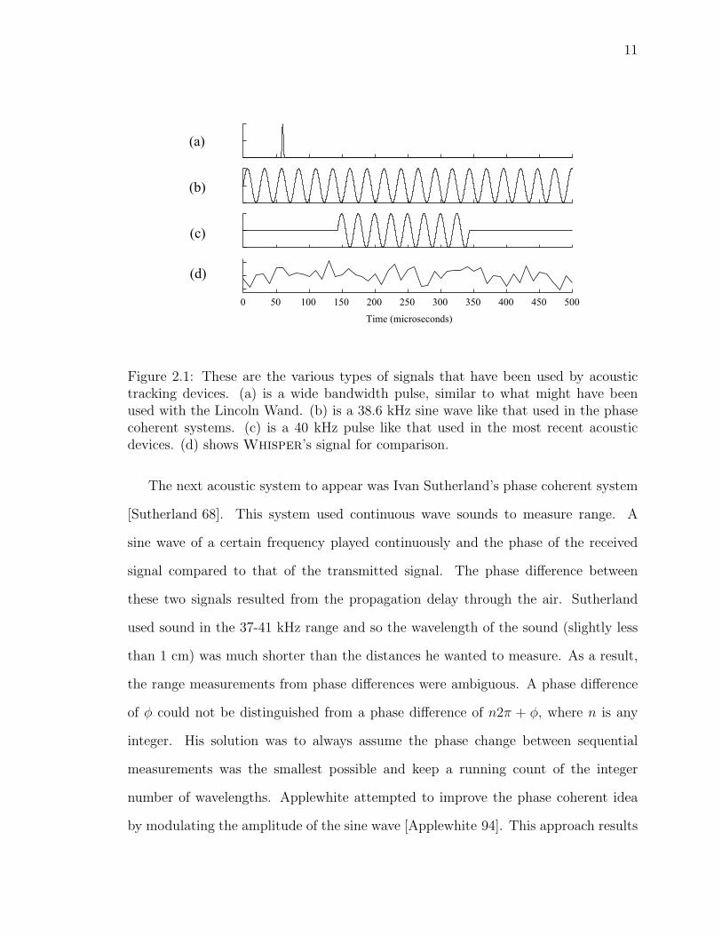
continuous wide bandwidth pseudonoise signal (see Figure 2.1). The first acoustic
system was the Lincoln Wand [Roberts 66]. This system used a pen with an ultrasonic
emitter to create a wide bandwidth pulse of sound (20 kHz to 100 kHz). The system
measured the time for this pulse to reach each of four microphones and then used
the speed of sound to calculate a range to each microphone. This approach has two
problems: limited sampling rate, and susceptibility to noise.
Since the Lincoln Wand used sound pulses, one pulse was indistinguishable from
another. This means that it was necessary to wait for the echoes of one pulse to fade
before creating the next pulse, which could take many milliseconds depending on the
environment. Related to this, only one sound source could be transmitting at a time.
If the Lincoln Wand had used two pens, each with an ultrasonic source, they would
have had to take turns transmitting, effectively halving the update rate of each. The
other issue is that this system could not distinguish between certain noises in the
environment and the pulse of sound. Any sufficiently broadband pulse-like sound,
such as a hand clap, could be mistaken for a pulse.
11
0 50 100 150 200 250 300 350 400 450 500
Time (microseconds)
(a)
(d)
(c)
(b)
Figure 2.1: These are the various types of signals that have been used by acoustictracking devices. (a) is a wide bandwidth pulse, similar to what might have beenused with the Lincoln Wand. (b) is a 38.6 kHz sine wave like that used in the phasecoherent systems. (c) is a 40 kHz pulse like that used in the most recent acousticdevices. (d) shows Whisper’s signal for comparison.
The next acoustic system to appear was Ivan Sutherland’s phase coherent system
[Sutherland 68]. This system used continuous wave sounds to measure range. A
sine wave of a certain frequency played continuously and the phase of the received
signal compared to that of the transmitted signal. The phase difference between
these two signals resulted from the propagation delay through the air. Sutherland
used sound in the 37-41 kHz range and so the wavelength of the sound (slightly less
than 1 cm) was much shorter than the distances he wanted to measure. As a result,
the range measurements from phase differences were ambiguous. A phase difference
of φ could not be distinguished from a phase difference of n2π + φ, where n is any
integer. His solution was to always assume the phase change between sequential
measurements was the smallest possible and keep a running count of the integer
number of wavelengths. Applewhite attempted to improve the phase coherent idea
by modulating the amplitude of the sine wave [Applewhite 94]. This approach results

12
in a signal with three sines (at the carrier frequency and both the sum and difference
of the carrier and modulating frequencies). This signal contains ambiguities that are
farther apart than just the carrier frequency alone. Depending on the choice of carrier
and modulating frequencies, the ambiguities can move to the point where they are
farther apart than the distance to be measured.
Phase coherent systems allow measurements to be taken more frequently, but they
do not solve the other issues faced by the Lincoln Wand. Echoes in the environment
add to the signal due to superposition, and since they are of the same frequency, pro-
duce a sine wave with different phase and/or amplitude. This results in an incorrect
range estimate. Also, any external noise at that frequency can result in erroneous
range measurements for the same reason.
Most modern acoustic tracking systems (such as [Foxlin 98b], [Foxlin 00]) use
a narrow bandwidth pulse in the ultrasonic range (typically in the range of 40-45
kHz). Transducers that function at this frequency tend to be narrow bandwidth
(approximately 5 kHz) and so the pulse of sound becomes narrow bandwidth. The
advantage is that the sound is inaudible, but these systems have the same problems
as the broadband pulse systems, namely low update rate and high sensitivity to noise.
As one example, the sound of jingling keys has significant frequency content in this
ultrasonic range.
One additional problem that all ultrasonic systems face is occlusion. At ultrasonic
frequencies, objects placed between the emitter and sensor block the sound thereby
preventing the calculation of a range. However, as I will discuss in Chapter 3, low
frequency sound diffracts around objects and can address this issue in acoustic sys-
tems. A further difficulty mentioned previously is the variation of the speed of sound
with atmospheric conditions. One method of determining the speed of sound is to
over-constrain the position of the target and solve for the speed of sound. The accu-
13
racy of the sound speed is not so important if the distances travelled are kept small,
such as near the body. This is simply because a certain percentage error in the speed
of sound results in a smaller incremental range error when compared to ranging over
long distances. The final difficulty mentioned is the acoustic noise that exists in typ-
ical environments where people work. Whisper resolves this last issue by borrowing
technology from the communications world.
2.3 Spread Spectrum Tracking Systems
The communications community has had to deal with echoes (referred to as multi-
path interference) and noise in developing communications systems. This has lead
to the development of spread spectrum techniques to solve these problems. As the
tracking community faces similar problems, it makes sense to leverage this knowledge
to improve tracking systems.
The application of spread spectrum to tracking systems is not a new idea. The
Global Positioning System (GPS) is probably one of the best known spread spectrum
tracking devices. GPS is an electromagnetic system that uses the microwave region
of the spectrum to measure ranges to a constellation of satellites orbiting the Earth
[Kaplan 96]. Combining four or more of these range measurements allows a user to
determine his or her location almost anywhere on the planet. Although well known
and highly useful, GPS operates on an entirely different scale from the systems dis-
cussed in this dissertation. However, the Whisper system operates in a manner
similar to GPS. Both use a spread spectrum signal to calculate ranges from a target
to known locations and then combine the measurements to produce the 3D location
of the target.
Bible mentions the idea of using spread spectrum in virtual-environment scale
tracking systems. Although he designs no specific system, Bible discusses building

14
a system from commercial GPS hardware[Bible 95]. One fully working spread spec-
trum tracking system for use in virtual environment scale applications is Spatiotrack
[Iltanen 98], [Palovuori 00]. This system works in the near-infrared portion of the
electromagnetic spectrum. Spatiotrack consists of 3 infrared light sources, each sur-
rounded by a rotating cylindrical mask. The mask creates a temporal pattern of
light that can be detected by a computer-mouse-size sensing device. Measuring the
time delay between the sensed light pattern and that of a reference measured at the
beacon, Spatiotrack determines the angle from each beacon to the sensor. The three
angles are combined to find the 3D location of the sensor. The key to the system is in
the design of the rotating masks. The pattern on the mask is a pseudo-noise pattern
that has an extremely useful autocorrelation function. I will return to this concept
in Chapter 3.
The Coda System uses a similar idea, but turned around. In this system, the mask
is fixed permanently above an imaging device. The tracking target is an infrared LED
and its light casts a shadow of the mask on to the imaging device[Charnwood 00].
The position of the shadow can be determined very accurately due to the mask’s
autocorrelation function. This measurement directly corresponds to the angle to the
target.
Another interesting spread spectrum tracking device has been under development
for some time by Ætherwire [Fleming 95]. This system is made up of a collection
of radio frequency transceivers that are capable of measuring the range to other
transceivers, very similar to GPS, but on a meter scale, not global scale. The spider
web of connections that results can be used to calculate the position of any one of
the locators with respect to any other.
I know of only a few acoustic systems that operate with spread spectrum sig-
nals. Richards implemented a spread spectrum acoustic ranging system as an ap-

15
plication of noise-locked-loop-based entrainment [Richards 00]. However, this system
only measured range and operated solely in the ultrasonic range. A company called
VTT automation claims to have developed a room-based tracking system using ultra-
sonic pseudonoise signals and correlation to find the position of a target in the room
[VTT Automation 01].
Although oriented towards a different application, a group of students developed
an acoustic, spread-spectrum radar system as a class project [Boman 00]. This system
used a chirp signal to find ranges to various objects in a room. It was not capable of
identifying a specific object, only of reporting ranges to objects in its field of view. It
was also designed to operate in a “snapshot” mode and not continuously.
Finally, and most similar to Whisper, is the acoustic ranging system described
by Girod and Estrin [Girod 01] which uses a pseudonoise acoustic signal to calculate
range between multiple elements of an ad-hoc deployable sensor network. One element
of the network simultaneously transmits the acoustic signal and a radio signal to
indicate the start time of the transmission. They use the difference between the
arrival times of the radio and acoustic signals to calculate the time of flight of the
acoustic signal. Similar to the radar system mentioned above, the acoustic signal is
not continuous and so the ranges are not calculated as frequently as with Whisper.
2.4 Body-centered Tracking Systems
The idea of tracking in a body-centered coordinate system has been largely ignored
in virtual environment research. This is most likely due to the need of determining
head position and orientation in the lab environment. As this has been the more im-
portant issue, much research has gone into it. However, with the development of sys-
tems such as the UNC HiBall [Welch 01] and Intersense’s Constellation [Foxlin 98b],
there are very good head-tracking devices available. For the purposes of tracking the
16
hands and feet of a virtual environment user, it makes a great deal of sense to track
these with respect to the user’s body. This simplifies the rendering of an avatar and
the use of hand positions in gestural interfaces such as [Mine 97] as the results are
already in the coordinate frame where they would be used. Furthermore, if the user’s
position is not needed with respect to the environment, a body-centered tracking
system needs no external infrastructure to function. All the necessary hardware can
be located on the user’s body.
There have been a few systems that do use a body-centered coordinate system.
Mechanical exoskeletons such as the Gypsy system [Meta Motion 00] and the more
flexible ShapeTape by Measurand, Inc. [Measurand Inc. 00] are body-centered simply
by construction. A human being’s limbs are all attached to the torso, so it makes
sense in an exoskeleton to have the torso be the fixed base of the mechanical arms.
Intersense is also working on a head-centered, pulse-based acoustic tracking system
as an interface to wearable computers [Foxlin 00]. Bachman developed a system
of inertial and magnetic sensors capable of determining body pose [Bachman 01].
Finally, some room-based tracking systems have been modified for use in a body-
centered fashion. Researchers at UNC used a magnetic tracking device to track a
user’s head, hands and shins relative to their torso and so were able to draw an
avatar of the user in a virtual environment [Insko 01].

Chapter 3
Spreading and Shaping the
Spectrum
Whisper takes advantage of ideas from the field of spread spectrum communica-
tions to avoid the difficulties faced by past systems, most importantly the slow update
rates, low noise tolerance, and inability to deal with occlusions.
This chapter begins with a brief description of communication systems in order
to introduce the topic of multiple access on communication channels. The following
section introduces the various approaches to spread spectrum communications. Next
is a discussion of a spread spectrum technique particularly suited for use with Whis-
per. Finally, I discuss the application of spread spectrum techniques to the acoustic
domain.
3.1 General Communications Principles
The point of communication is to move information between two points. These two
points are labeled to define the direction of information flow as source and destination.
The information travels over a physical medium called the channel. A source creates
a signal (be it electric, radio, or acoustic) and transmits it over the channel. The

18
destination observes the state of the channel and converts these observations into
data. The source controls the amplitude and frequency content of the signal at any
given point in time. However, more than one source using a channel may result in
the sources interfering with one another. This can lead to problems if the channel
is, for example, free space being used as a channel for radio signals. Scientists and
engineers developed techniques to allow multiple sources to share a channel. This is
called multiple access.
The three major multiple access techniques are frequency-division multiple access
(FDMA), time-division multiple access (TDMA), and code-division multiple access
(CDMA). In FDMA each source uses a portion of the channel’s frequency spectrum.
Radio and television stations are good examples of FDMA. Each station limits its
transmissions to a specific range of frequencies. Users listen to different stations by
adjusting the range of frequencies their television or radio uses as input. Furthermore,
this is the general technique chosen by the Federal Communications Commission to
divide the radio spectrum in the United States.
Time-division multiple access methods schedule the sources to take turns using
the channel. This is generally how people talk to each other. First one person says
something and the other listens. Then the other speaks while the first listens. This
is also the method used by cars when sharing a common resource (an intersection
between two roads). Cars from one of the roads use the intersection for a while then
the traffic lights change and the cars on the other road use the intersection.
The final multiple-access technique is CDMA. In this technique all sources trans-
mit at once, using the same frequency range. The receivers selectively listen to one
source by knowing how the information was transmitted—by knowing the “code”.
This is similar to a group of people simultaneously speaking in different languages.
If you want to hear what one person is saying you would listen to the English, if

19
you want to hear what another is saying you might listen to German. Knowing the
language the person is speaking is similar to knowing the code that is being used to
transmit a CDMA signal.
CDMA is a very convenient technique as a source can transmit its signal whenever
and at whichever frequency it would like, but it causes some problems. The biggest of
these is that the communication has to be very robust to noise on the channel. This is
because the transmissions of other sources sharing the channel appear as noise to any
receiver that does not know their codes. Typical narrow bandwidth communications
methods, such as Amplitude Modulation (AM), are not tolerant of this level of noise.
These methods assume that if there is any signal in their frequency range that it is
part of the desired signal. CDMA requires a communications method that is more
robust to noise. Spread spectrum communications was developed for just this reason.
3.2 What Does Spread Spectrum Mean?
Spread spectrum systems transmit information using a bandwidth that is much
larger than the bandwidth of the information being transmitted. A typical system
might use a transmission bandwidth that is 1000 times larger than the information
bandwidth. This approach results in many advantages such as greater noise immunity.
A greater noise immunity also means that the signal is more difficult to jam. Another
benefit of the increased noise immunity is that a weaker signal can be used, making it
more difficult for someone to detect and therefore intercept the signal. Finally, spread
spectrum systems are also able to take advantage of selective addressing (transmitting
to separate groups of receivers instead of broadcasting to all receivers) and code-
division multiple access [Dixon 84].

20
3.3 Classification of Spread Spectrum Schemes
There are four typically used spread spectrum methods. They are [Dixon 84]:
• frequency hopping: Pick a set of carrier frequencies and jump between them
according to a pseudo-random pattern.
• time hopping: Transmit at specific times for short durations according to a
pseudo-random pattern
• pulsed-FM/chirp: Sweep the carrier over a wide frequency band during the
pulse interval
• direct sequence (DS): Modulates a carrier by a digital code running at a much
higher rate than the information being transmitted.
Spread spectrum methods can use any of the multiple access methods described
in the previous section. However, given their noise tolerance they are very well suited
to CDMA. This technique is convenient because the signal sources do not have to be
coordinated with one another. In TDMA the sources need to be synchronized and in
FDMA they need to negotiate the assignment of frequency bands.
3.4 A Closer Look at Direct Sequence CDMA
Whisper uses CDMA because signal sources do not need to coordinate resource
use, allowing the sources to be simpler. Further, the system uses direct sequence
because it is easily implemented on a fixed-rate digital system. The other multiple
access and spread spectrum techniques will not be discussed further.
A typical direct sequence system generates a code that it uses to modulate a carrier
frequency. It is also possible to use the code directly in what is called a baseband

21
system (the approach taken by Whisper). In either situation this code plays a very
important role in the system and its selection strongly influences system performance.
The next section discusses these codes and how they are selected.
3.4.1 Pseudonoise codes
The codes typically used by direct sequence systems are binary sequences called
pseudonoise because to an outside observer they appear noise-like even though they
are deterministic.
The ideal code has an autocorrelation function that is an impulse function. This
allows the code to have maximal correlation with a non-delayed version of itself and
not interfere with itself if a portion of it appears in the signal at a different delay
(through multi-path interference or a repeating jammer). The discussion that follows
describes important classes of binary pseudonoise codes. However, Whisper does
not use these binary codes but uniform random sequences generated by Matlab. This
is for a variety of reasons that I describe in detail in Section 5.3.2.
The most important codes in use are the maximal length sequences. These codes
have nearly an impulse function autocorrelation and are easily generated using linear
feedback shift registers. To generate a maximal length sequence, a shift register is
initialized to all ones. Specific bits of the shift register are selected and their contents
summed (modulo 2). This result is pushed into the shift register and the bit that
comes out the other end is used as the current code bit (see Figure 3.1). A single bit
of the code is commonly referred to as a “chip”.
The key element to this approach is the selection of the register bits (also called
taps) to sum. When the taps are selected properly, this system generates a repeating
binary sequence 2n − 1 bits long. This is why the code is called a maximal length
sequence. It is the longest sequence an n bit register can generate. Incidentally, since

22
1 11
1 2 3 4 5 6 7 80.0
1.5
-6 -5 -4 -3 -2 -1 0 1 2 3 4 5 6-1
3
7(a) (b)
(c)
Figure 3.1: Maximal length sequences can be generated by linear shift registers (a).The resulting maximal length sequence (b) has an autocorrelation function (c) thatis nearly an impulse function. It’s value is 2n−1 at 0 offset and -1 at all other offsets.
an n bit register can represent 2n values, the one that is missing is all zeros. This is
logical since if the register contained all 0s the sum of any number of them would be
0 and the contents of the register would remain the same iteration after iteration.
Maximal length sequences are the optimal sequences to use in an environment
with only one source. However, there are situations in which other codes are useful.
The first of these is the situation where there are multiple sources. In this case two
maximal-length sequences are not guaranteed to have small cross-correlation which
means that one of the signals could interfere with another. One solution to this
problem is the use of Gold codes[Dixon 84]. They are made from multiple maximal
sequences added together. They have guaranteed maximum cross-correlations that
are very low to limit interference.
23
Another situation that calls for a different code is long-distance ranging. A com-
mon situation is measuring the position of a space probe that is far from Earth. This
requires the use of a very long code so that it does not repeat in the time it takes
to get back to Earth, which would result in an ambiguous range measurement. The
problem with this code is that it is very difficult to calculate exactly where in the code
the signal currently is without prior information. As a result, codes such as the JPL
ranging codes have a shorter, more frequently repeating portion to allow faster, but
multi-stage, synchronization with the code[Dixon 84]. This introduces the important
issue of acquiring and tracking a Direct Sequence signal.
3.4.2 Acquiring and decoding a DS signal
The ideal method for acquiring a direct sequence signal is to know the range to
the transmitter, an exact time for when the source began transmitting and an exact
current time. With this information, the current code position of the received signal
can be calculated. However, in a realistic system not all these pieces of information
are known. In the case of Whisper it is the range that is unknown at the beginning.
The typical acquisition method used when precise information is not available is
to scan through all possible code positions until the correct delay is found. Detection
is simple in general due to the strong correlation at the correct delay. However, the
impulse-like autocorrelation means that the tested location has to be very near the
actual location in order to produce any hint of the delay. Furthermore, scanning
through the entire code can take a long time, especially if the code is long as in the
space probe application mentioned in the previous section. In this case the code can
be billions of bits long making such a search impossible in practice. The code used by
Whisper and the distances involved are both short enough that such a brute force
approach is practical, though computationally expensive.

24
Given this difficulty with acquisition, it is highly undesirable to lose synchroniza-
tion with the code on the incoming signal. This means tracking the current delay of
the signal is very important. The most commonly used algorithms are the tau-dither
loop and the delay-lock loop.
The tau-dither loop works by rapidly switching between a delayed and non-delayed
version of the local code (usually 1/10th of a code bit apart). The code sample chosen
is multiplied by the current input sample and the result integrated. This output is
one point on the correlation curve. Since the code sample used is constantly switched,
the output value jumps between two different points on the correlation peak. If one
is greater than the other then the algorithm moves the delay estimate towards the
corresponding code bit in order to climb the peak. If they are equal then the peak
must be between them, and the algorithm does not change its estimate.
The delay-lock loop multiplies two different locally-generated code samples (1/2
chip ahead and 1/2 chip behind the current estimated delay) by the incoming signal
simultaneously and integrates the result. Comparing the two values results in a
modification of the delay estimation similar to the tau-dither loop. Clearly, these two
tracking algorithms use essentially the same approach. The delay-lock loop is merely
a parallelized version of the tau-dither loop.
Both of these algorithms have been designed for direct implementation in hard-
ware. Whisper was planned from the beginning to do as much work as possible in
software, for the flexibility this provides. As a result, it is possible to use a more
sophisticated algorithm. Whisper uses a combined correlation/Kalman filter algo-
rithm for tracking the code delay, as I will describe in Chapter 4.
Once the system is synchronized with the incoming signal’s code, the signal can be
decoded by performing the inverse of the function the transmitter used to modulate
the signal with the code. The simplest technique used is inverting the phase (phase
25
shifting by 180 degrees, also called Bi-Phase Shift Keying or BPSK) of the carrier for a
1 bit and doing nothing for a 0 bit in the code. This stage does not occur in Whisper
as there is no data being transmitted over the signal. The system only tracks the
current delay of the incoming signal compared to the outgoing signal. Chapter 4 will
discuss this further.
3.5 Wide Bandwidth Signals in Acoustic Tracking
So why use spread spectrum in an acoustic tracker? Spread spectrum handles
the two big acoustic tracker problems. The interference rejection properties of spread
spectrum remove much of the noise that the environment adds to the signal. Echoes
also become a less significant issue as most are easy to separate from the desired
signal. Figure 3.2 illustrates this last point. All echoes show up as peaks with longer
path lengths than the peak corresponding to the direct path length. The only echoes
that remain a problem are those whose paths are less than a few chip times longer
than the direct signal path. In this case the peaks in the correlation are too close
together and impossible to isolate.
In addition to solving these problems, there are two other important benefits
from using CDMA. First, it allows multiple transmitters to work simultaneously and
therefore allows concurrent distance estimates between all transmitters and receivers.
This parallelization speeds up the system response. Also, by suitable selection of
the frequency band for the spread spectrum signals, the physical properties of sound
propagation can be exploited, as elaborated next.

26
5 0 5 10 15 20 25
0
0.5
1
Cor
rela
tion
Val
ue
Correlation Offset
Figure 3.2: Multi-path interference is easy to separate from the signal in direct se-quence systems. The left-most peak in the correlation corresponds with the directpath between transmitter and sensor. All peaks to the right of the first peak are dueto echoes.
3.5.1 Low Frequencies Allow Diffraction
By allowing the wide bandwidth acoustic signal to contain low frequencies, Whis-
per can take advantage of the diffraction of sound. Most acoustic trackers function in
the ultrasonic range so that they are inaudible, but this also makes occlusion a prob-
lem. Any object coming between the ultrasonic transmitter and receiver blocks the
sound. In reality, it is not that the higher frequencies do not diffract, but that they
do not diffract enough to be of use. However, by using lower frequencies, the sound
can diffract enough around the object to allow the tracker to continue functioning.
The diffraction phenomenon is fairly common and most people have probably
observed it. Imagine talking to someone who is around the corner of a building.
Even if there are no nearby surfaces for your voice to reflect from, the person will
still be able to hear you due to the diffraction of your voice around the corner of the
building.

27
(a)
(c)
(b)
Shadow boundary
Figure 3.3: A sound wave grazing the surface of a sphere (a) creates a creeping wave(b) at the tangent point. As the creeping wave travels along the surface of the sphereit sheds waves (c) into the shadow zone behind the sphere.
Most of the occluding objects for a body-centered tracking device would be parts
of the human body. Spheres and cylinders are the most similar geometric objects to
parts of the human body (e.g., head is mostly spherical and arms are cylindrical). As
such, the sound will tend to meet these objects in a tangential way leading to surface
diffraction (as opposed to wedge diffraction that occurs around corners). As the sound
grazes the surface of the occluder, a portion of the sound follows along the surface of
the occluder. This is commonly referred to as a “creeping wave”. This creeping wave
exists in the shadow region (where ray acoustics would indicate there should be no
sound). As the creeping wave travels along the surface it sheds rays in a direction that
is tangential to the current point on the surface (see Figure 3.3). The shed rays and
the incoming rays behave as is normally expected of sound. However, the creeping
wave attenuates in a different fashion as it travels along the surface due to both
divergence of the creeping wave and losing energy through shedding diffracted rays
[Keller 62]. Given this mechanism for diffraction, the reason that occluders appear
to block higher frequencies is that creeping waves attenuate much more rapidly at
higher frequency [Neubauer 68].

28
(a)
(b)
(c)
Figure 3.4: Ultrasound (a) is blocked when there is an occlusion between the trans-mitter and sensor. However, a low frequency signal (b) diffracts around the obstacle.The trade-off is a longer path length and weaker signal than the direct route (c) thatexists when there is no occlusion.
The tradeoff when using diffraction is that it makes the path length longer than
the direct path between the transmitter and receiver (see Figure 3.4). This results in
a range measurement with more systematic error. However, if the alternative is to get
no signal and therefore be unable to estimate the target position, this is acceptable.
Using diffraction lowers the accuracy of the tracker but allows it to continue operating
while occluded.
3.5.2 High Frequencies Yield Precision
Whisper also benefits from the use of higher frequency components of the spread
spectrum signal. The low frequencies may diffract, but even un-occluded they do not
allow high resolution tracking. Permitting more high frequency content in the signal
allows Whisper to use a higher chip rate which means more code bits to correlate
with in a finite amount of time. More code bits in a finite time period result in a finer
determination of signal delay and therefore a finer resolution distance measurement
(see Figure 3.5).

29
5 4 3 2 1 0 1 2 3 4 5
0
0.5
1
5 4 3 2 1 0 1 2 3 4 5
0
0.5
1Cor
rela
tion
Val
ue
Correlation Offset (seconds * 10 )
(a)
(b)
-4
Figure 3.5: Using a signal that contains higher frequencies results in a narrowercorrelation peak. This allows for more accurate determination of time delay. (a)limited to 50 kHz (b) limited to 10 kHz
3.6 Spectrum Shaping
One disadvantage of having sound waves capable of effectively diffracting around
objects is that they are audible to Whisper’s users. However, the exact spectrum
can be shaped so as to remove the most annoying components in the audible range.
Through personal experience, I have found these to be the lower frequency compo-
nents, below 1 kHz. The added advantage of ignoring this portion of the spectrum
is that it contains most of the acoustic noise present in typical environments (e.g.,
human voices and fan noise).
Further, the low signal-to-noise ratio needed for a spread spectrum system to
function means that the low frequency components of the signal do not have to be
loud. The low frequencies could be attenuated more than the high frequencies or
removed altogether when there is no occlusion.
Of course shaping of the wide bandwidth signal must have some effect on the
operation of the system. The effect presents itself in the shape of the autocorrelation

30
50 40 30 20 10 0 10 20 30 40 500. 5
0
0.5
1
Correlation Offset
Cor
rela
tion
Val
ue
0 10 20 30 40 50 60 70 80 90 100� 0.5
0
0.5
1
time (samples)
Out
put
� 50 � 40 � 30 � 20 � 10 0 10 20 30 40 50� 0.5
0
0.5
1
Correlation Offset
Cor
rela
tion
Val
ue
(a)
(b)
(c)
Figure 3.6: Filtering the pseudonoise signal changes the shape of the correlationfunction. (a) the autocorrelation of the original pseudonoise (b) the impulse responseof the filter used to produce filtered pseudonoise (c) the autocorrelation of the filteredpseudonoise
of the output signal. Whisper’s spectrum shaping is created with a filter, resulting
in the correlation taking on the shape of the code’s auto-correlation run through this
filter twice (once in the forward direction and once in the reverse direction—essentially
the non-causal form of the filter) as shown in Figure 3.6.
Chapter 4
Range Measurement and Occlusion
This chapter discusses the simplest version of Whisper, a one-dimensional or
range measurement system and how occlusion affects it. Chapter 5 expands these
ideas to transform Whisper into a three-dimensional tracker. This chapter begins
by discussing the hardware needed for the system, followed by a description of the al-
gorithm that implements the range measurement. The chapter ends with a discussion
of the impact of occlusions on range measurements.
4.1 System Configuration
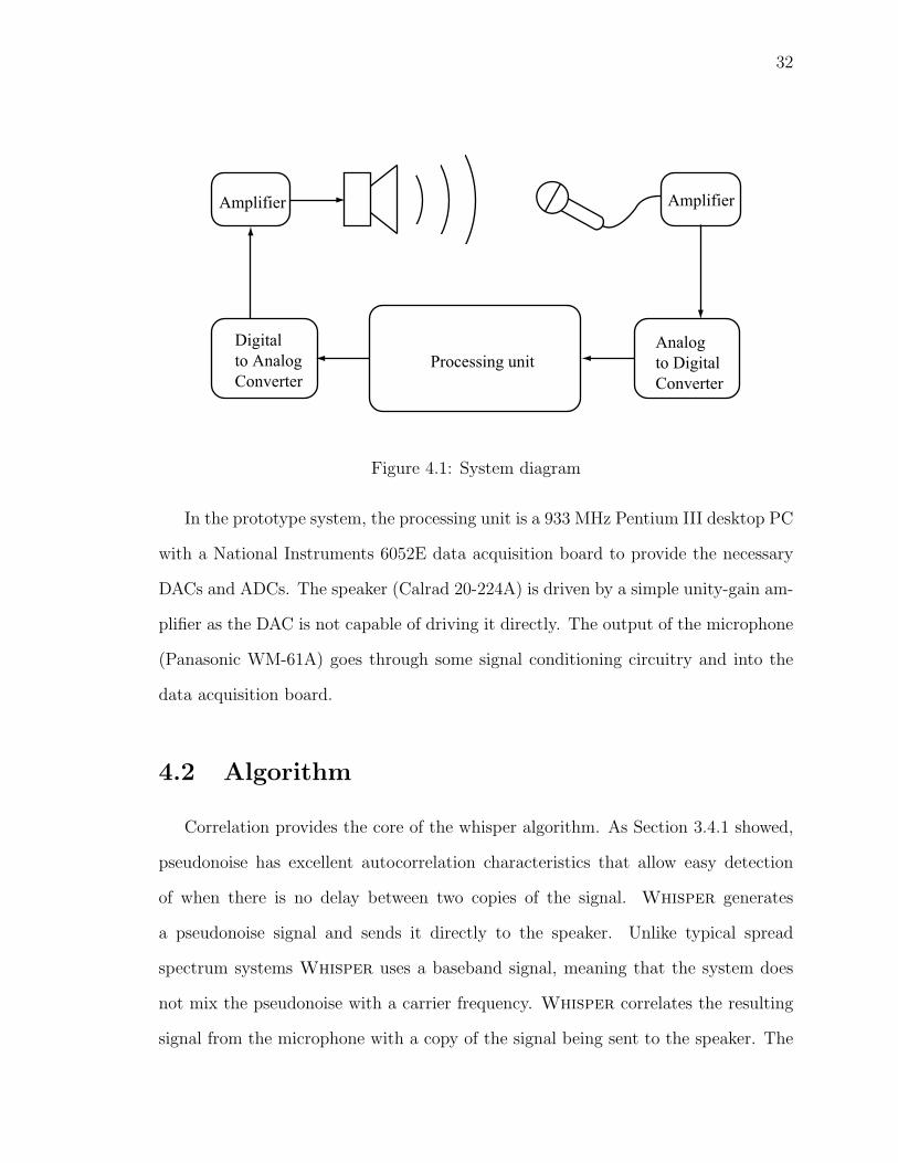
Whisper’s hardware consists of three parts: a processing unit, a speaker, and
a microphone. The processor generates the appropriate signal, converts it to analog
with a digital to analog converter (DAC), amplifies the result, and sends the signal to
the speaker. The speaker converts the electrical signal into an acoustic signal. The
acoustic signal propagates through the air to the microphone. The microphone con-
verts the acoustic signal back into an electrical signal. The output of the microphone
is sent through an amplifier and filter, an analog to digital converter (ADC) and back
to the processing element (see Figure 4.1).
32
Amplifier
Digitalto AnalogConverter
Analogto DigitalConverter
Amplifier
Processing unit
Figure 4.1: System diagram
In the prototype system, the processing unit is a 933 MHz Pentium III desktop PC
with a National Instruments 6052E data acquisition board to provide the necessary
DACs and ADCs. The speaker (Calrad 20-224A) is driven by a simple unity-gain am-
plifier as the DAC is not capable of driving it directly. The output of the microphone
(Panasonic WM-61A) goes through some signal conditioning circuitry and into the
data acquisition board.
4.2 Algorithm
Correlation provides the core of the whisper algorithm. As Section 3.4.1 showed,
pseudonoise has excellent autocorrelation characteristics that allow easy detection
of when there is no delay between two copies of the signal. Whisper generates
a pseudonoise signal and sends it directly to the speaker. Unlike typical spread
spectrum systems Whisper uses a baseband signal, meaning that the system does
not mix the pseudonoise with a carrier frequency. Whisper correlates the resulting
signal from the microphone with a copy of the signal being sent to the speaker. The
33
propagation time between the speaker and the microphone delays the incoming signal.
As a result, the peak appears at a correlation offset dependent on the delay. Since
the ADC samples the signal at a constant rate, Whisper can convert this offset into
a delay time by dividing by the sampling rate. The final step is to convert the delay
time to distance by multiplying by the speed of sound.
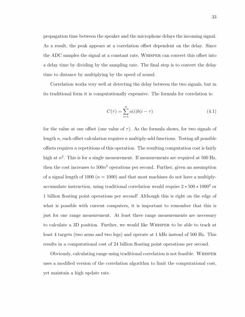
Correlation works very well at detecting the delay between the two signals, but in
its traditional form it is computationally expensive. The formula for correlation is:
C(τ) =n∑
i=1
a(i)b(i− τ) (4.1)
for the value at one offset (one value of τ). As the formula shows, for two signals of
length n, each offset calculation requires n multiply-add functions. Testing all possible
offsets requires n repetitions of this operation. The resulting computation cost is fairly
high at n2. This is for a single measurement. If measurements are required at 500 Hz,
then the cost increases to 500n2 operations per second. Further, given an assumption
of a signal length of 1000 (n = 1000) and that most machines do not have a multiply-
accumulate instruction, using traditional correlation would require 2 ∗ 500 ∗ 10002 or
1 billion floating point operations per second! Although this is right on the edge of
what is possible with current computers, it is important to remember that this is
just for one range measurement. At least three range measurements are necessary
to calculate a 3D position. Further, we would like Whisper to be able to track at
least 4 targets (two arms and two legs) and operate at 1 kHz instead of 500 Hz. This
results in a computational cost of 24 billion floating point operations per second.
Obviously, calculating range using traditional correlation is not feasible. Whisper
uses a modified version of the correlation algorithm to limit the computational cost,
yet maintain a high update rate.

34
Kalman Filter (Predictor)
Kalman Filter (Corrector)
Reduced Correlation with computation reuse
Traditional Correlation to initialize
Figure 4.2: The Whisper algorithm consists of a Kalman filter combined with acorrelation stage that reuses previous computation results.
4.2.1 Description
The central methods Whisper uses to reduce the computation cost are limiting
the offset search space, and reducing the computation cost per offset. If the approx-
imate location of the correlation peak is known, the algorithm need search only a
portion of the offset space. To accomplish this, a Kalman filter estimates the current
position of the peak, given past measurements and a model for the target’s motion.
Whisper reduces the computation cost per offset by maintaining partial results from
previous iterations for reuse. Figure 4.2 shows an overview of the complete Whisper
algorithm.
Kalman Filter
Here I present the portion of the Whisper algorithm involving the Kalman filter.
Figure 4.3 contains pseudocode for this portion of the algorithm.
35
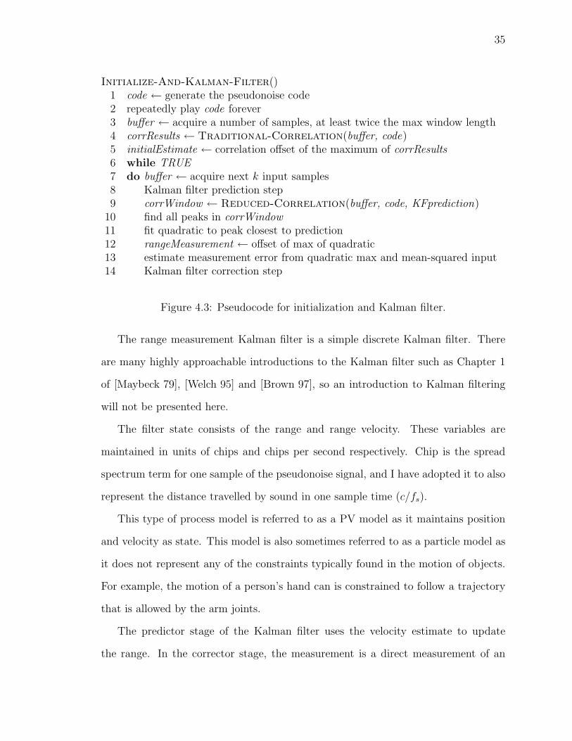
Initialize-And-Kalman-Filter()1 code ← generate the pseudonoise code2 repeatedly play code forever3 buffer ← acquire a number of samples, at least twice the max window length4 corrResults ← Traditional-Correlation(buffer, code)5 initialEstimate ← correlation offset of the maximum of corrResults6 while TRUE7 do buffer ← acquire next k input samples8 Kalman filter prediction step9 corrWindow ← Reduced-Correlation(buffer, code, KFprediction)
10 find all peaks in corrWindow11 fit quadratic to peak closest to prediction12 rangeMeasurement ← offset of max of quadratic13 estimate measurement error from quadratic max and mean-squared input14 Kalman filter correction step
Figure 4.3: Pseudocode for initialization and Kalman filter.
The range measurement Kalman filter is a simple discrete Kalman filter. There
are many highly approachable introductions to the Kalman filter such as Chapter 1
of [Maybeck 79], [Welch 95] and [Brown 97], so an introduction to Kalman filtering
will not be presented here.
The filter state consists of the range and range velocity. These variables are
maintained in units of chips and chips per second respectively. Chip is the spread
spectrum term for one sample of the pseudonoise signal, and I have adopted it to also
represent the distance travelled by sound in one sample time (c/fs).
This type of process model is referred to as a PV model as it maintains position
and velocity as state. This model is also sometimes referred to as a particle model as
it does not represent any of the constraints typically found in the motion of objects.
For example, the motion of a person’s hand can is constrained to follow a trajectory
that is allowed by the arm joints.
The predictor stage of the Kalman filter uses the velocity estimate to update
the range. In the corrector stage, the measurement is a direct measurement of an
36
internal state variable (the range). Assume a generic process model for a continuous
time Kalman filter
x = Fx + Gu (4.2)
where
x =
r
r
(4.3)
is the state variable containing range (r) and range velocity (r), u is a scalar process
noise, and
F =
0 1
0 0
(4.4)
G =
0
1
(4.5)
Further, assume a measurement model
z = Hx + v (4.6)
where z is a scalar measurement, v is a scalar measurement noise, and
H =[
1 0
](4.7)
To re-state the model in words, the current range is the previous range plus the
integrated velocity since the last range update. The process noise enters solely through
the range velocity state variable. Finally, the measurements used to update the filter
are direct measurements of the range state variable.

37
I transform the filter into discrete form using standard methods. The general form
of the discrete model is then
xi+1 = Aixi + wi (4.8)
where Ai is the state transition matrix and wi is the process noise with covariance
matrix Qi. Whisper’s state transition and noise covariance matrices are independent
of time and so the i subscripts on both are dropped. Given a uniform sampling rate
fs and the number of samples (k) between filter iterations, A is
A =
1 k/fs
0 1
(4.9)
The exact value of Q depends on the target dynamics and allows tuning of the filter.
I discuss the selection of the measurement noise covariance (R) in Section 4.2.2 along
with the process model noise covariance (Q).
The filter obtains its initial values from a traditional correlation algorithm. The
correlation offset that contains the largest value is the initial range in chips. Using
the assumption that the target is not moving during initialization, the range velocity
is set to 0 chips per second. Further, the initial value of the error covariance matrix
is set to
P =
1 0
0 0
(4.10)
in units of chips squared. The target should not be moving during initialization so a
variance of 0 is appropriate for the velocity variance. The initial value for the range is
also assumed to be within 1 chip of the actual range (otherwise the peak correlation
value would have appeared elsewhere) so an initial value of 1 for the variance is
sufficient to start the filter. It quickly converges to the actual value.
38
After initialization, the Kalman filter’s prediction of the current range is an input
to a reduced correlation computation. Centered around the filter’s estimate, the
correlation routine computes only a limited number of offsets. Normally, the filter
prediction should not be off by more than one chip, but to ensure that signal lock is
not lost, which will occur if the correlation peak moves outside the search range, a
sufficient number of offsets are searched. This number is a parameter of the algorithm
and will be discussed in Section 4.2.2.
Whisper finds all the peaks in the reduced correlation result (see Figure 4.4).
Each peak in this search range (defined as a value with lesser or equal values on both
sides) becomes input to a quadratic peak finder. This is done by taking the peak
value along with its left and right neighbors and fitting a quadratic function to the
three values. Figure 4.5 shows a typical result of this step. The peak’s location is
at the maximum of the quadratic. The quadratic with the largest maximum is the
desired peak, and the offset of its maximum is used as the range measurement. The
Kalman filter takes this range measurement and uses it for the correction step.
Computation Reuse
In one version of the Whisper algorithm, the system used a correlation window
size of 1000 samples and computed one iteration of the Kalman filter every 100 input
samples. Using the normal correlation algorithm, this meant that 900 of the 1000
input samples in the window for the current iteration were used in the previous
iteration. If the target is still and thus the algorithm is computing over the same
range of offsets, then this represents a large waste of computing resources through
re-calculating the same values. Thus, Whisper uses a form of common subexpression
elimination and breaks the correlation computation into chunks of length k. Figure 4.6
contains pseudocode describing how this is accomplished.

39
25 30 35
-0.5
0
0.5
1
Correlation Offset
Cor
rela
tion
Val
ue
Figure 4.4: Whisper computes the correlation in a local area around the Kalmanfilter prediction. The algorithm searches this region for peaks, indicated here bydotted lines.
25 30 35
-0.5
0
0.5
1
Correlation Offset
Cor
rela
tion
Val
ue
Figure 4.5: After the peaks are found, Whisper fits a quadratic to each and findsthe maximum size peak. In this case the largest peak is the same as the largest peakin the raw correlation, but sometimes a different quadratic peak is larger than thelargest raw correlation peak.
40
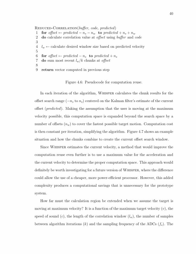
Reduced-Correlation(buffer, code, predicted)1 for offset ← predicted − ns − nw to predicted + ns + nw
2 do calculate correlation value at offset using buffer and code34 lw ← calculate desired window size based on predicted velocity56 for offset ← predicted − ns to predicted + ns
7 do sum most recent lw/k chunks at offset89 return vector computed in previous step
Figure 4.6: Pseudocode for computation reuse.
In each iteration of the algorithm, Whisper calculates the chunk results for the
offset search range (−ns to ns) centered on the Kalman filter’s estimate of the current
offset (predicted). Making the assumption that the user is moving at the maximum
velocity possible, this computation space is expanded beyond the search space by a
number of offsets (nw) to cover the fastest possible target motion. Computation cost
is then constant per iteration, simplifying the algorithm. Figure 4.7 shows an example
situation and how the chunks combine to create the current offset search window.
Since Whisper estimates the current velocity, a method that would improve the
computation reuse even further is to use a maximum value for the acceleration and
the current velocity to determine the proper computation space. This approach would
definitely be worth investigating for a future version of Whisper, where the difference
could allow the use of a cheaper, more power-efficient processor. However, this added
complexity produces a computational savings that is unnecessary for the prototype
system.
How far must the calculation region be extended when we assume the target is
moving at maximum velocity? It is a function of the maximum target velocity (v), the
speed of sound (c), the length of the correlation window (lw), the number of samples
between algorithm iterations (k) and the sampling frequency of the ADCs (fs). The

41
IterationKalman filter prediction
i
i-1
i-2
i - l / k + 1
..
....
..
.57
55
55
56
Column Sums
Correlation Offsets
w
..
....
50 51 52 53 54 55 56 57 58 59 60 61 62
Chunk in the offset search range
Chunk in expanded calculation range Window used for peak fitting
Figure 4.7: In each iteration of the algorithm, Whisper computes partial correla-tion results based on the most recent Kalman filter state and set of input samples.Whisper then sums the chunks to create the correlation results for the offset searchwindow.
maximum number of chips by which the peak will shift between iterations (nc) is
nc = kv
c(4.11)
To get the number of chips the peak could shift over the entire window, nc is multiplied
by the number of iteration-size chunks that fit in one window:
nw = nclwk
= kv
c
lwk
=v
clw (4.12)
As long as the offset calculation range is increased by nw on each side of the offset
search range, then it can be guaranteed that the correct correlation chunks will be
available when needed.
In order for this computation reuse to improve the calculation performance, the
correlation window length must exceed the number of samples between iterations by

42
a significant margin. For example, if the correlation window length is chosen as 1000
samples and there are 1000 samples between iterations, there will be no overlap of
computation. However, if there are only 100 samples between algorithm iterations,
then 900 out of the 1000 samples used in the correlation window will be the same as
the previous iteration, and the computation reuse is beneficial.
This last example is very close to the actual parameter set for Whisper and
provides a useful comparison to the computation cost of correlation. The cost for the
same window size (1000) and an update rate of 1000 Hz using traditional correlation is
2 billion operations per second. Using the Kalman filter, but not computation reuse,
and searching a window of 7 offsets, the cost is reduced to 1000 ∗ 7 ∗ 2 ∗ 1000 = 14
million operations per second. Then, including the computation reuse while skipping
100 samples and assuming a maximum velocity of 1% of the speed of sound requires an
expanded offset computation range of 27 offsets. Computing the cost in this situation
results in 1000 ∗ 27 ∗ 2 ∗ 100 = 5.4 million operations per second—a huge savings over
traditional correlation even considering the added computation cost of the Kalman
filter.
Locating the Peak
In describing Whisper’s algorithm I stated that it uses the Kalman filter pre-
diction to produce a set of correlation values to search for a peak. At that point I
indicated that Whisper uses a quadratic fit to the peak data in order to find the
location of the peak to a greater precision than the spacing between correlation val-
ues. Why use a quadratic and not some other model for the shape of the peak? After
all, the autocorrelation of the pseudonoise sequence seems to show the peak with a
triangular shape (see Figure 4.8).
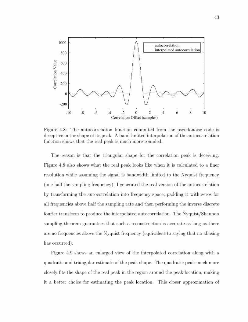
43
-10 -8 -6 -4 -2 0 2 4 6 8 10
-200
0
200
400
600
800
1000
Correlation Offset (samples)
Cor
rela
tion
Val
ue
autocorrelationinterpolated autocorrelation
Figure 4.8: The autocorrelation function computed from the pseudonoise code isdeceptive in the shape of its peak. A band-limited interpolation of the autocorrelationfunction shows that the real peak is much more rounded.
The reason is that the triangular shape for the correlation peak is deceiving.
Figure 4.8 also shows what the real peak looks like when it is calculated to a finer
resolution while assuming the signal is bandwidth limited to the Nyquist frequency
(one-half the sampling frequency). I generated the real version of the autocorrelation
by transforming the autocorrelation into frequency space, padding it with zeros for
all frequencies above half the sampling rate and then performing the inverse discrete
fourier transform to produce the interpolated autocorrelation. The Nyquist/Shannon
sampling theorem guarantees that such a reconstruction is accurate as long as there
are no frequencies above the Nyquist frequency (equivalent to saying that no aliasing
has occurred).
Figure 4.9 shows an enlarged view of the interpolated correlation along with a
quadratic and triangular estimate of the peak shape. The quadratic peak much more
closely fits the shape of the real peak in the region around the peak location, making
it a better choice for estimating the peak location. This closer approximation of

44
-0.25 -0.2 -0.15 -0.1 -0.05 0 0.05 0.1 0.15 0.2 0.25900
950
1000
1050
1100
Correlation Offset (samples)
Cor
rela
tion
Val
ue
interpolated correlationtriangle peak fitquadratic peak fit
Figure 4.9: Using a quadratic to estimate the peak location is more accurate thanusing a triangular model because the quadratic more closely models the peak shape.
the quadratic function, in addition to its low computational cost when compared to
bandwidth-limited interpolation, is why Whisper uses a quadratic to calculate a
precise peak location.
4.2.2 Selecting Parameters
In describing the Whisper algorithm I mentioned a number of parameters, and
they all present opportunities to tune the behavior of the algorithm. The parameters
are the correlation window length, the size of the search window, the number of
samples between iterations of the algorithm, and the Kalman filter error covariance
matrices (Q and R).
Correlation Window Length
The correlation window length must be chosen so as to provide enough benefit from
the correlation (a larger window will result in a larger peak above the background
noise, allowing more precise and accurate delay determination). However, as the

45
window grows larger, it introduces more latency and becomes less capable of handling
doppler shift. The answer is to use the longest window that is possible given the
expected doppler calculated from the target’s expected motion characteristics.
In this case, the target of primary interest is a human being’s hand. Typical “fast”
hand motion occurs at 3 m/s [Atkeson 85]. Adding a safety margin, I assume the
maximum velocity to be 3.5 m/s, or approximately 1% of the speed of sound (c). By
assuming that this motion occurs along a radius from the microphone, the worst case
doppler effect occurs. The effect of doppler shift is to spread out the peak with the
amount of spreading proportional to the window length and target velocity. Since
doppler is due to motion of the target, the delay changes and therefore the correlation
peak moves over the length of the correlation window. If the window is too short, the
peak will get lost in the background noise. If the window is too long, the peak will
smear out over many offsets and begin to look like background noise. The optimum
window length is one that both maximizes the size of the peak and minimizes the
peak smearing. In a perfect setting (infinite bandwidth and no background noise)
I discovered this to be in the range of 2 to 3 times the number of chips it takes
for the doppler shift to produce a 1 chip shift in the input signal. Using a window
smaller than this does not allow the peak to reach its maximum size while a window
larger than this does not increase the peak size, only its width. Once again assuming
a maximum speed of 1% of c (1 chip shift in 100 chips), this means the minimum
window length Whisper uses is 200 chips.
Conveniently, the Kalman filter provides an estimate of the current velocity. Us-
ing this velocity, the length of the window is dynamically selected to keep its length
between 2 and 3 times the “1 chip shift in x chips” length. Furthermore, a maxi-
mum window size of 1000 is used to limit latency and the amount of computation.

46
This length provides an adequate correlation peak, easily distinguishable from the
surrounding noise.
Offset Search Window Size
The size of the search window (ns) is somewhat arbitrary. The size needed is
almost completely defined by the accuracy with which the Kalman filter predicts the
peak location. If the Kalman filter is 100% accurate then the search area only needs
to be 3 samples wide (enough to give the three data points to the quadratic peak
fitting algorithm). However, experience has shown that this is not sufficient when
using a PV model for the motion of a person’s hand.
One rule that seems to work well is to make the window large enough to fit the
entire peak (approximately 3 chips wide when the target is still). This is especially
important when there is doppler shift in the signal. In this case the peak widens out
and forms a plateau instead of a sharp peak. Noise on the input is sufficient to make
the peak location jump around on this plateau. As long as the whole peak fits into
the offset search window, then when the doppler shift stops, the true peak will still be
in the window. The dynamic window sizing limits the peak width to approximately
twice that of the peak when there is no target velocity. Given this and adding one
additional chip in each direction as insurance, the search window is set at −4 to +4
chips (9 chips total), centered on the Kalman filter’s predicted location.
Number of Samples Between Iterations
There is a trade-off between computation cost and the number of samples between
iterations. Here I create a formula representing this trade-off, and discuss interpreting
the formula to find the most efficient point in the computation space. Unfortunately,
there is no minima to the function and so the most efficient point is also dependent
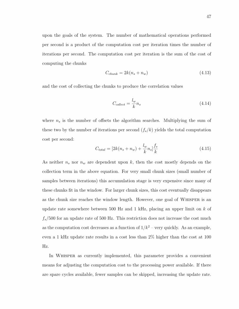
47
upon the goals of the system. The number of mathematical operations performed
per second is a product of the computation cost per iteration times the number of
iterations per second. The computation cost per iteration is the sum of the cost of
computing the chunks
Cchunk = 2k(ns + nw) (4.13)
and the cost of collecting the chunks to produce the correlation values
Ccollect =lwk
ns (4.14)
where ns is the number of offsets the algorithm searches. Multiplying the sum of
these two by the number of iterations per second (fs/k) yields the total computation
cost per second:
Ctotal = [2k(ns + nw) +lwk
ns]fs
k(4.15)
As neither ns nor nw are dependent upon k, then the cost mostly depends on the
collection term in the above equation. For very small chunk sizes (small number of
samples between iterations) this accumulation stage is very expensive since many of
these chunks fit in the window. For larger chunk sizes, this cost eventually disappears
as the chunk size reaches the window length. However, one goal of Whisper is an
update rate somewhere between 500 Hz and 1 kHz, placing an upper limit on k of
fs/500 for an update rate of 500 Hz. This restriction does not increase the cost much
as the computation cost decreases as a function of 1/k2 – very quickly. As an example,
even a 1 kHz update rate results in a cost less than 2% higher than the cost at 100
Hz.
In Whisper as currently implemented, this parameter provides a convenient
means for adjusting the computation cost to the processing power available. If there
are spare cycles available, fewer samples can be skipped, increasing the update rate.

48
Increasing the update rate also keeps the Kalman Filter more accurate as it receives
more frequent measurements. A final aspect to consider (although merely an imple-
mentation issue) is the ease of combining the chunks into the desired window length.
Given a set of possible skip intervals, one which divides the window length evenly is
preferable.
Kalman Filter Parameters
The final parameters are the most difficult to decipher. Many people refer to
Kalman filter tuning as something of an art. Exact values can be computed only in
the simplest cases with fully known and understood process models, something that
is just not possible for human motion. In fact, the proper form of the process model
for human motion is not known. The PV model is frequently used because it is a
good balance between simplicity and performance. Also, the optimal values for these
parameters vary with the environment, the particular user of the system, and the
current background noise level. The best approach is to choose values for the average
situation.
I calculated the noise on the range measurements by collecting a number of data
sets with a speaker and microphone located fixed distances apart (20, 40, 60, and 80
cm). I used 8 different signal to noise ratios at each distance, varying this parameter
by playing the tracking signal and a separate, uncorrelated noise signal at various
volumes. This was done in a fairly quiet office environment (additional noise came
from the fans of two PCs and the ventilation system). I computed an estimate of the
noise to signal ratio as
NSR =1lw
∑lwi=1 input2i
(pcorr/lw)2(4.16)
where lw is the length of the correlation window, input is a vector containing the most
recent lw input values and pcorr is the correlation value at the peak.
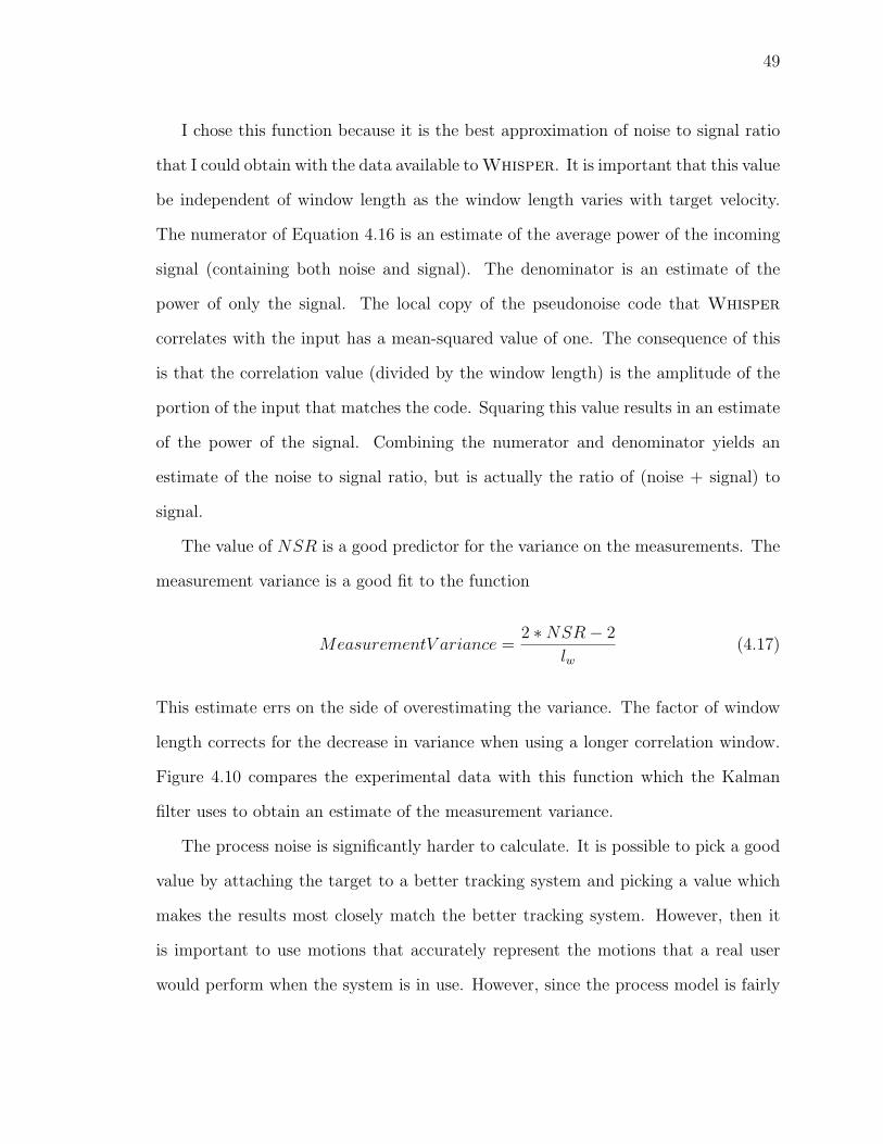
49
I chose this function because it is the best approximation of noise to signal ratio
that I could obtain with the data available to Whisper. It is important that this value
be independent of window length as the window length varies with target velocity.
The numerator of Equation 4.16 is an estimate of the average power of the incoming
signal (containing both noise and signal). The denominator is an estimate of the
power of only the signal. The local copy of the pseudonoise code that Whisper
correlates with the input has a mean-squared value of one. The consequence of this
is that the correlation value (divided by the window length) is the amplitude of the
portion of the input that matches the code. Squaring this value results in an estimate
of the power of the signal. Combining the numerator and denominator yields an
estimate of the noise to signal ratio, but is actually the ratio of (noise + signal) to
signal.
The value of NSR is a good predictor for the variance on the measurements. The
measurement variance is a good fit to the function
MeasurementV ariance =2 ∗NSR− 2
lw(4.17)
This estimate errs on the side of overestimating the variance. The factor of window
length corrects for the decrease in variance when using a longer correlation window.
Figure 4.10 compares the experimental data with this function which the Kalman
filter uses to obtain an estimate of the measurement variance.
The process noise is significantly harder to calculate. It is possible to pick a good
value by attaching the target to a better tracking system and picking a value which
makes the results most closely match the better tracking system. However, then it
is important to use motions that accurately represent the motions that a real user
would perform when the system is in use. However, since the process model is fairly

50
0 100 200 300 400 500 600 700 800 9000
200
400
600
800
1000
1200
1400
1600
1800
(noise + signal)/signal (estimated power)
Var
ianc
e of
rang
e m
easu
rem
ents
* w
indo
w le
ngth
(chi
ps2 )
Measurement Variance as a Function of Noise to Signal Ratio
Figure 4.10: Whisper uses the function described by the line to perform onlineestimation of the measurement variance. The points are the measurement variancecalculated from experimental data.

51
simple, the meaning of the process noise is fairly clear and the process noise can be
changed to suit the situation.
In the range measurement Kalman filter, the value of Q is like a knob that, turned
one way (decreased Q), makes the range estimate less noisy but also makes the tracker
less responsive (increased filtering), while turned the other way (increased Q) makes
the tracker more responsive but have a noisier output (decreased filtering). Another
option is to use a multiple model Kalman filter that selects between a tuning for still
situations and a tuning for more dynamic situations.
4.3 Dealing With Occlusion
A body-centered tracking device must be capable of handling occlusions. This
is due to the wide range of hand motion a human being is capable of. There is no
possible placement of emitter/sensor pairs (with one on the torso and the other on
a hand) such that a clear line of sight is always available. In addition, the normal
actions a person performs can lead to the occlusion of an emmitter/sensor pair. The
Whisper user could pick up an object or put their hand behind a fixed obstacle in
the environment.
If Whisper used the typical ultrasonic approach to acoustic tracking, it would
not be suitable for use in these scenarios as any occluding object would block the
ultrasound. However, because Whisper makes use of lower frequency sound, enough
diffraction occurs around many occluding objects, such as a person’s arm, to allow
the system to continue tracking.

52
4.3.1 Effect of Occlusion on Signal
When an occluder moves between the speaker and microphone, the acoustic sig-
nal no longer travels a straight path between the two. Instead, as I describe in
Section 3.5.1, the sound travels along a tangent to the occluder, then along the sur-
face of the occluder and is shed at the point which the path to the microphone is
tangent to the occluder. This increases the distance travelled by the sound (thereby
increasing the delay). In addition, all frequencies are not attenuated equally along
this path. The amplitude of the signal decreases with distance w along the occluder’s
surface as [Pierce 81]
e−αw
√w
(4.18)
where α is the attenuation coefficient (units of nepers per meter). The value for α is
given by
α = f 1/3αc (4.19)
where f is the frequency in hertz and αc is the remainder of the coefficient that is
independent of frequency and constant for a given physical scenario. As this equa-
tion indicates, higher frequency creeping waves attenuate more quickly and therefore
diffraction acts as a low-pass filter on the signal (see Figure 4.11).
It is easy to observe this effect on actual signals by looking at a spectrogram
(graph of frequency content versus time) of a signal while an occluder passes through
the signal path. Figure 4.12 shows the spectrogram of the signal from a microphone
while a 10.16 cm radius styrofoam sphere is passed through the straight line path
between the speaker and microphone. Notice how the higher frequencies disappear,
especially as the sphere enters the path at approximately 8 seconds and exits the path
at approximately 18 seconds.

53
0 5 10 15 20 25 30 35 40 45 50-20
-15
-10
-5
0
Frequency (kHz)
Atte
nuat
ion
(dB
)
w = 1 cmw = 2 cmw = 4 cm
Figure 4.11: Frequency dependency of the attenuation of creeping waves. Valuesare from theory for creeping waves travelling 1, 2, and 4 cm along the surface of aperfectly rigid sphere with a radius of 10 cm. Note that the shape is that of a low-passfilter.
Time (s)
Freq
uenc
y (k
Hz)
0 5 10 15 20 250
10
20
30
40
50
Figure 4.12: A spectrogram showing that the higher frequencies disappear when aspherical occluder blocks the direct path between speaker and microphone (darkercolor corresponds to higher magnitudes at that frequency). Notice how some of themiddle frequencies return when the sphere is exactly on the direct path, acting as anacoustic lense.

54
An interesting property of the spectrogram in Figure 4.12 is that some of the
middle frequencies return (and are even amplified) when the center of the sphere is
on the straight-line path between the speaker and microphone. This is due to the
many paths the sound may take around an occluder in three dimensions and still reach
the microphone. These paths are all of different length and so appear as multipath in
most situations. However, when the object is spherical and its center is on the direct
path between speaker and microphone then all the diffracted signals are of the same
path length and constructively add to create a stronger signal than exists without
the sphere there. Of course this only occurs for frequencies at which the magnifying
effect exceeds the attenuation of the creeping waves.
4.3.2 Effect of Occlusion on Correlation
Given the observation that occlusion acts like a low-pass filter on the acoustic
signal, how does this affect the correlation? In Section 3.6 I describe how a filter
applied to the pseudonoise code affects the autocorrelation of the code. In this case
I am interested in the effect of a filter applied only to the transmitted signal, but
not the original code. It is easiest to see the effect of such a filter on the correlation
by looking at the signals in the frequency domain. Given a pseudonoise code c and
a filter (with impulse response h) that is applied to it, possibly due to diffracting
around an occluder, the resulting signal is
input = c ∗ h (4.20)
with ∗ denoting the convolution function. Taking the Fourier transform of this func-
tion results in
F{input} = F{c} · F{h} (4.21)
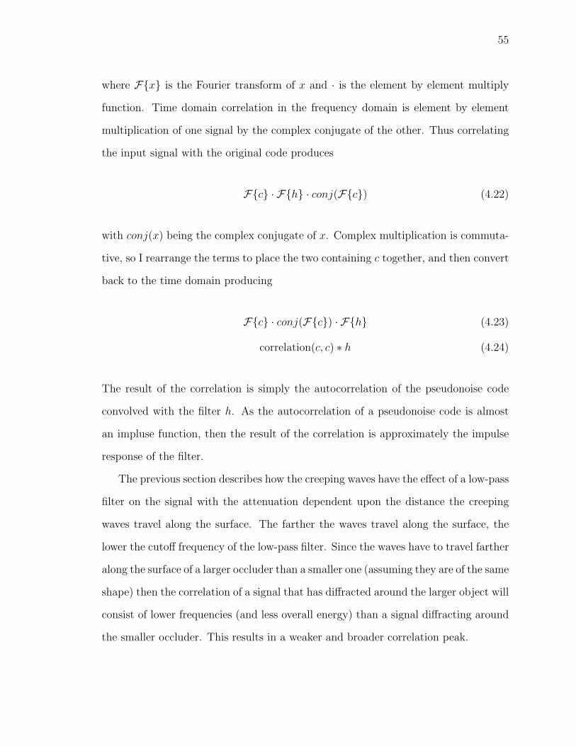
55
where F{x} is the Fourier transform of x and · is the element by element multiply
function. Time domain correlation in the frequency domain is element by element
multiplication of one signal by the complex conjugate of the other. Thus correlating
the input signal with the original code produces
F{c} · F{h} · conj(F{c}) (4.22)
with conj(x) being the complex conjugate of x. Complex multiplication is commuta-
tive, so I rearrange the terms to place the two containing c together, and then convert
back to the time domain producing
F{c} · conj(F{c}) · F{h} (4.23)
correlation(c, c) ∗ h (4.24)
The result of the correlation is simply the autocorrelation of the pseudonoise code
convolved with the filter h. As the autocorrelation of a pseudonoise code is almost
an impluse function, then the result of the correlation is approximately the impulse
response of the filter.
The previous section describes how the creeping waves have the effect of a low-pass
filter on the signal with the attenuation dependent upon the distance the creeping
waves travel along the surface. The farther the waves travel along the surface, the
lower the cutoff frequency of the low-pass filter. Since the waves have to travel farther
along the surface of a larger occluder than a smaller one (assuming they are of the same
shape) then the correlation of a signal that has diffracted around the larger object will
consist of lower frequencies (and less overall energy) than a signal diffracting around
the smaller occluder. This results in a weaker and broader correlation peak.

56
-10 -8 -6 -4 -2 0 2 4 6 8 10-6
-4
-2
0
2
4
6
Correlation Offset (from calculated peak location)
Cor
rela
tion
Val
ue (*
10e-
3)
No occlusion5.1 cm sphere10.2 cm sphere15.2 cm sphere20.3 cm sphere
Figure 4.13: Larger obstacles filter out more of the tracking signal than smallerobstacles. This results in a shorter and wider correlation peak.
Figure 4.13 shows this result with real signals. The magnitude of the correlation
peak decreases as larger obstacles (in this case spheres) occlude the direct path be-
tween speaker and microphone. Notice that the peak is still there in all cases, although
with a greatly reduced amplitude for the larger occluders. Whisper calculates the
range from the peak as normal and continues to track.
4.3.3 Effect of Occlusion on WHISPER
As the previous section showed, there is still a correlation peak to track even
when there are occlusions between the speaker and the microphone. As Whisper
tracks these peaks in the correlation, it operates no differently during occlusions.
The difference is entirely in Whisper’s misinterpretation of the range measurements.
Whisper does not know there is an occluder in the way and so continues to believe
that the range corresponding to the tracked peak location is the straight-line distance
between the speaker and the microphone. Of course without knowledge of at least the
location and shape of the occluder, Whisper cannot interpret the range measurement

57
Direct Calculated MeasuredRadius Range Diffracted Range Diffracted Range Difference(cm) (cm) (cm) (cm) (cm)
2.54 64.28 64.48 64.53 +0.055.08 64.28 65.08 65.20 +0.127.62 64.28 66.10 66.30 +0.2010.16 64.28 67.52 67.68 +0.16
Table 4.1: Comparison of measured and theoretical diffracted path lengths around asphere
correctly. As such, an occlusion introduces error into the range measurement given
to the Kalman filter.
The maximum error in range for a particular occluder can easily be calculated
by using the ray model for diffraction that I have described. Assuming a spherical
occluder that is located midway between the speaker and the microphone and located
on the straight-line path between the two, the length of the diffracted path is
ddiff = 2
√√√√(d
2
)2
− r2 + r(sin−1
(2r
d
)) (4.25)
where d is the length of the straight-line path and r is the radius of the sphere.
I have done the above calculation for spheres of radius 2.54, 5.08, 7.62 and 10.16
cm. I took the straight-line path length from a set of experiments I did putting real
styrofoam spheres in the path of a range-measurement Whisper system. Table 4.1
compares the calculated diffraction path lengths to those reported by Whisper.
There are many sources for the error between the two diffracted path lengths. The
most significant of these are
• the spheres might not have been half way between the speaker and microphone
(position could have been up to 2 cm closer to either the speaker or the micro-
phone)

58
• the sphere’s center might not have been exactly on the direct path between
the speaker and microphone (center of the sphere could have missed passing
through the direct path by up to 2 mm)
• the spheres are not perfect spheres (the radii may vary by ±2 mm for the largest
sphere)
• the speaker is not a point source for the acoustic signal (speaker is approxi-
mately a square 2 cm on a side). However, since the extent of the speaker was
perpendicular to the direct path between speaker and microphone, it probably
did not affect the path length much.
I modified the diffracted path length equation to take these sources of error into
account. The resulting equation is
ddiff = e + f + g + h (4.26)
where the summed terms are
e =
√√√√(d
2+ x
)2
+ y2 − r2 (4.27)
f = r
π
2− cos−1
r√(d2
+ x)2
+ y2
− tan−1
(y
d2
+ x
) (4.28)
g = r
π − cos−1
r√(d2− x
)2+ (y − z)2
− tan−1
(y − zd2− x
) (4.29)
h =
√√√√(d
2− x
)2
+ (y − z)2 − r2 (4.30)
with d and r defined as previously and the additional variables defined as indicated in
Figure 4.14. Given these formulas, I calculated the sensitivity of the diffracted path

59
d/2
d
xyz
e h
f g
speaker
microphone
Figure 4.14: Diagram explaining the variables in the equation for the length of adiffracted path around a sphere.
Sphere Sphere Not Sphere Off Radius SpeakerRadius Centered Direct Path Variations Size∣∣∣∂ddiff
∂x· 2.0
∣∣∣ ∣∣∣∂ddiff
∂y· 0.2
∣∣∣ ∣∣∣∂ddiff
∂r· 0.2
∣∣∣ ∣∣∣∂ddiff
∂z· 1.0
∣∣∣(cm) (cm) (cm) (cm) (cm)
2.54 0.0 0.03 0.03 0.085.08 0.0 0.06 0.06 0.167.62 0.0 0.09 0.10 0.2410.16 0.0 0.13 0.13 0.32
Table 4.2: Maximum possible effect of the four error sources. All partial derivativeswere evaluated at the configuration where there is no error (i.e., x, y, and z are all 0)and then multiplied by the maximum error for each source
length to each of the error sources using the maximum values indicated in the above
list. The analysis shows that the differences between the measured and calculated
diffracted path lengths are all within the estimated experimental error. Table 4.2
summarizes the results.
Chapter 5
Three-Dimensional Tracking and
Multiple Targets
The previous chapter only dealt with the simple situation of one speaker and one
microphone. This chapter covers changes made to the system to allow Whisper to
capture the 3-dimensional position of the target and tracking multiple targets.
This chapter starts by discussing the combination of multiple range measurements
to form a fully three-dimensional system. Then I describe how the system performs.
I conclude by exploring a Whisper system tracking multiple targets.
5.1 Calculating 3D Position
In order to calculate the 3D position of the target, Whisper needs range mea-
surements between the target and at least three different known locations. For this
section I assume that a speaker is attached to the target and three microphones are
at fixed locations (to match the current Whisper implementation). Section 5.3 on
multiple targets discusses the relative advantages and disadvantages of this decision.
The simplest way to view the calculation of the three-dimensional position of the
tracking target is as the replication of the one-dimensional system. Results from three

61
separate Kalman filters as described in Chapter 4 could be combined to yield the 3D
position. In actual implementation, the algorithm is more tightly integrated, but this
provides a good conceptual model.
One way to visualize the combination of the ranges (although not the method
Whisper uses) is as the intersection of three spheres. Three spheres can intersect in
0, 1 or 2 points as long as no pair of spheres is concentric. The case of 0 intersections
should not occur, except in the case of a ranging error. The case of 1 intersection
happens only in very rare situations where two of the spheres meet tangentially. The
general case is the situation where there are two intersections. Given the proper
location of the three microphones with respect to the desired tracking volume, there
will be one solution which can be thrown out as impossible. The three microphones
define a plane and the two solutions are mirror images of each other on opposite sides
of this plane. As long as the desired tracking volume is entirely on one side of this
plane, then the proper solution is easy to determine as it’s the one that lies in “front”
of the plane.
The coordinate system in which the target’s position is defined is then described
by the location of the three microphones. At the minimum they must be non-collinear
to properly define a 3D position, but the locations affect the system performance as
I describe in Section 5.2.2.
If the ranging systems are simply duplicated as indicated above, Whisper would
have three separate Kalman filters, along with an additional algorithmic step to com-
bine the results from the three filters. A better solution is to modify the Kalman filter
to estimate the 3D position of the target and from that estimate the three ranges.

62
5.1.1 Modifications to the Kalman Filter
The Kalman filter’s state for three-dimensional tracking contains the (X, Y, Z)
position of the target along with the velocities in each of these dimensions. One large
difference from the one-dimensional case is that the measurements (ranges to the fixed
microphones) are nonlinear functions of the (X, Y, Z) position of the target. A system
with a nonlinear measurement function such as this can not use the standard discrete
Kalman filter. The filter requires some type of linearization of the measurement func-
tion. Whisper does this by using an extended Kalman filter. An extended Kalman
filter linearizes around the estimated position trajectory. As only the measurement
function is nonlinear, this only affects the measurement update (corrector) step of the
Kalman filter. One aspect of the extended Kalman filter to be cautious of is the error
introduced by the linearization. I discuss this in the next section (Section 5.1.2).
The predictor step of the Kalman filter is still linear and so is largely unchanged
from the one-dimensional filter. The difference is that now there are three position
and three velocity state variables corresponding to the (X, Y, Z) position and velocity
of the target. The continuous time process model remains the same
x = Fx + Gu (5.1)
although with
x =
x
x
y
y
z
z
(5.2)

63
as the state variable and
F =
0 1 0 0 0 0
0 0 0 0 0 0
0 0 0 1 0 0
0 0 0 0 0 0
0 0 0 0 0 1
0 0 0 0 0 0
(5.3)
G =
0
qx
0
qy
0
qz
(5.4)
The measurement model, however, has changed and now is
z = h(x, v) (5.5)
The function h(x, v) is a non-linear function of the state variable x. Specifically, it is
h(x, v) =√
(xx −mx)2 + (xy −my)2 + (xz −mz)2 + v (5.6)
where m is the coordinates of the microphone to which the range is being calculated.
I transform these to their discrete forms as with the range-measurement Kalman
filter and get the following values for the state transition matrix and process noise
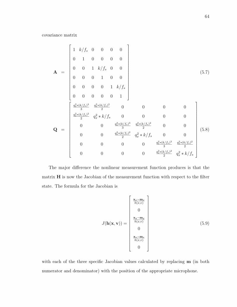
64
covariance matrix
A =
1 k/fs 0 0 0 0
0 1 0 0 0 0
0 0 1 k/fs 0 0
0 0 0 1 0 0
0 0 0 0 1 k/fs
0 0 0 0 0 1
(5.7)
Q =
q2x∗(k/fs)3
3q2x∗(k/fs)2
20 0 0 0
q2x∗(k/fs)2
2q2x ∗ k/fs 0 0 0 0
0 0 q2x∗(k/fs)3
3q2x∗(k/fs)2
20 0
0 0 q2x∗(k/fs)2
2q2x ∗ k/fs 0 0
0 0 0 0 q2x∗(k/fs)3
3q2x∗(k/fs)2
2
0 0 0 0 q2x∗(k/fs)2
2q2x ∗ k/fs
(5.8)
The major difference the nonlinear measurement function produces is that the
matrix H is now the Jacobian of the measurement function with respect to the filter
state. The formula for the Jacobian is
J(h(x,v)) =
xx−mx
h(x,v)
0
xy−my
h(x,v)
0
xz−mz
h(x,v)
0
(5.9)
with each of the three specific Jacobian values calculated by replacing m (in both
numerator and denominator) with the position of the appropriate microphone.
65
Whisper calculates the Jacobian at the estimated state of the filter after the time
update step. Since the three range measurements are independent of one another,
their respective measurement updates are performed sequentially to simplify the math
(doing all three at once would require a matrix inversion, while one at a time this
inversion becomes a division).
Except for these changes to the Kalman filter, Whisper’s 3-D algorithm is almost
identical to the range measurement case. The one difference is that the peak-finding
computation must be repeated once for each of the input signals from the three
microphones, but that process is exactly the same as for the range measurement
algorithm.
5.1.2 Error from Nonlinearity
As I describe in the previous section, Whisper uses an extended Kalman filter
to handle the nonlinear measurement function. However, this introduces some error
since only the function’s value and first derivative are used in estimating the nonlinear
behavior. How much error does this introduce?
Assuming that the target is travelling at a maximum speed of 3.5 m/s and that
the Kalman filter iterations occur at 1 ms intervals, the maximum distance the target
can travel between iterations is 3.5 mm. The maximum error in the function estimate
occurs when the motion is perpendicular to the direction of the range measurement.
In this instance, the Jacobian calculates the change in range to be 0 as the motion is
in a direction that is tangent to the sphere. However, the range does actually change,
and it changes a maximum of
dr =√
r2 + 0.00352 − r (5.10)
meters where r is the current range and 0.0035 m is the maximum distance the

66
microphone 2 microphone 3
microphone 1
Y
-Z
coordinate origin
30.48 cm
30.4
8 cm
Figure 5.1: Whisper’s microphone array is three microphones arranged in the shapeof a rotated ‘L’. They are positioned on the corners of a square 30.48 cm on a side.
user could travel between filter iterations. Dividing this through by r results in the
maximum fractional error from the linearization as a function of r
fractionalerror =
√r2 + 0.00352 − r
r(5.11)
Note that this function is large for very small ranges and falls off as a function of 1/r.
Further, the maximum error is less than 1% at a range of 2.2 cm and less than 0.01%
at a range of 20 cm.
5.2 Performance
I implemented Whisper as I have described in terms of both hardware and soft-
ware on a 933 MHz Pentium III desktop computer. A piece of clear acrylic holds
the three microphones in the arrangement shown in Figure 5.1. The origin of the
coordinate system is defined at the location of microphone 2. The X vector extends
perpendicular to the plane of the microphones. The Y vector extends towards micro-
phone 3, and the -Z vector extends towards microphone 1.

67
Whisper operates with the following parameters. The maximum window length
(lw) is 1000 samples, 100 samples are between algorithm iterations (k), the search
range (ns) is +/−4 offsets (extended by nw = 10 samples on each side), the sampling
rate is 100 kHz for both speaker and microphones, and Q is the value of Equation 5.8
after substituting the following values:
qx = 900 (5.12)
qy = 600 (5.13)
qz = 600 (5.14)
The interpretation of the q values is very similar to the 1D filter. However, in this case
each controls the filtering along one dimension of the target’s position instead of along
the range measurements. An interesting factor in the values I chose for Whisper
is that there is an asymmetry between the different dimensions. This is because
Whisper is better able to measure the position along the X vector than the other
two dimensions. Conceptually this makes sense as the three range measurements
are all very nearly measuring along this dimension, while the other two dimensions
rely on differences between the range measurements. A more formal understanding
of this asymmetry can be gained using the math describing the geometric dilution
of precision in Section 5.2.2. Given the above parameters, I will now discuss the
performance of Whisper.
5.2.1 Factors Affecting Performance
There are four main factors that influence the performance of Whisper. The
first of these is noise. Noise in the environment adds to the incoming pseudonoise
signal, producing a signal that no longer exactly matches the code. The quadratic
68
peak finder also introduces some error. As I mentioned in Section 4.2.1, the quadratic
is only an approximation of the peak shape and so does not match exactly. Another
source of error in Whisper is the directionality of the transducers. Although it would
be ideal to have truly omnidirectional transducers, such devices do not exist and so
the imperfections of these devices decrease the performance of Whisper. The final
factor is atmospheric conditions. As I mention in Section 2.2, temperature gradients
and air currents both affect the accuracy of Whisper.
Some of the factors mentioned above introduce some type of filtering on the signal.
It is possible to compensate for this filtering. The inverse filter could be applied to
the signal to allow the signal to match the code more closely and therefore produce a
better correlation signal. Some work would be required to figure out how to calculate
the inverse transforms. One unfortunate side effect of this approach would be the
amplification of any noise that added to the signal after the original filtering occurred.
Noise
The most important influence on the performance of Whisper is the background
noise. Section 4.2.2 showed the effect of gaussian noise on range measurements and
how the range measurement variance is predictable based on the noise to signal ratio.
Converting these range measurements to 3D positions involves two processes that
affect this variance. The first tends to increase the variance and is known as geometric
dilution of precision. I describe this in Section 5.2.2. The second tends to reduce the
variance and is the filtering introduced by the Kalman filter. The tradeoff involved
in filtering is increased latency—the measurements are less noisy, but are available
later in time.
Neither of these two factors control how much noise enters the range measurements
though. They merely amplify or reduce the amount of noise that already exists on
69
the range measurements. Instead it is the filtering performed by the transducers
(speakers and microphones) that control how noise enters the range measurements.
Extremely wide-bandwidth acoustic transducers are difficult to find. This is
mostly due to the range of frequencies human beings can perceive. When sound
is used, the designer of the system either wants the sound to be audible or inaudible
to humans. These two situations tend not to overlap and so most transducers have a
cutoff frequency (either high or low) in the neighborhood of 20 kHz.
The result of the bandwidth limitations of the transducers is that the pseudonoise
signal essentially passes through a bandpass filter created by the speaker and the
microphone. The devices are small so they do not have good low frequency response.
The high frequency cutoff is set by the bandwidth of the transducers. The end result
of this filtering is to change the shape of the correlation peak. Figure 4.13 showed
that as larger occluders remove more of the high frequencies from the pseudonoise
signal, the correlation peak shrunk and became flatter. Imagine noise being added
to these correlations. An amount of noise that would not really affect the shape of
the unoccluded peak in Figure 4.13 would be enough to entirely hide the peak that
results from the largest occluder. Essentially, the impulse response of the transducers
defines the sensitivity of the range measurements to noise and results in the variance
versus noise to signal ratio function shown in Figure 4.10.
Quadratic Peak Finder
The use of a quadratic peak finder introduces some error into the range measure-
ments. Embodied in this approach is the assumption that the shape of the correlation
peak is approximately that of a quadratic. The three points of the correlation closest
to the peak define a quadratic in order to calculate a fine resolution location of the
peak. As the quadratic shape is only an approximation, the location of the maxi-

70
mum of the quadratic is not guaranteed to be the same as the peak location and so
introduces some error.
However, it is a better approximation than the triangular peak that results from
assuming an infinite bandwidth system and therefore was selected as a good approach.
The actual shape of the peak is difficult to determine as it is dependent on a much
more complex set of state variables than it is reasonable to use to describe the system.
This includes the location of objects in the world around the microphone and speakers
that affect the available acoustic paths between the speaker and microphone.
In order to estimate the error from the quadratic peak approximation, I compared
the quadratic peak location estimate with the peak location in a sinc reconstruction
of the autocorrelation signal. The sinc reconstruction is the most accurate version
of the original signal that can be produced from the sample points. Theoretically
it should match the original continuous signal exactly as long as the signal is band-
limited to half the sampling rate. For Whisper this condition is almost certainly
met as the response of the speaker and microphone drops off sharply after 30 kHz,
and is insignificant by 50 kHz (half the 100 kHz sampling rate).
Using a 60 second data set of recorded human motion, I widened the computation
width of the correlation to +/- 25 samples. This created a larger number of sam-
ples to more accurately perform the sinc reconstruction. Figure 5.2 shows the delay
difference between the the quadratic estimate and the sinc reconstruction maximum
for a representative subset of the data set. Using the differences between all avail-
able measurement pairs (60 seconds * 1000 Hz * 3 range measurements = 180,000
measurement pairs), the mean error in the quadratic estimate is -0.049 chips (ap-
proximately 0.17 mm) and the standard deviation is 0.037 mm (implying that 99.7%
of the quadratic estimates have errors between -0.160 and 0.062 chips/-0.21 mm and
0.050 mm).

71
0 10 20 30 40 50 60-0.3
-0.25
-0.2
-0.15
-0.1
-0.05
0
0.05
0.1
time (seconds )
quad
ratic
est
imat
e - s
inc
peak
loca
tion
(chi
ps)
Figure 5.2: Example data showing the difference between the quadratic peak estimateand the peak location in a sinc reconstruction of the correlation function. This plotshows every 10th difference of the range measurement to microphone 2 from a 60second data set.
Directionality of Transducers
The transducers that Whisper uses (as with all acoustic transducers) suffer from
directionality. At higher frequencies the radiation patterns of the transducers become
more directional. The result is that the microphone receives less of the signal from the
speaker when the two are not aimed directly at one another. The higher frequencies
disappear first and more and more of the signal is filtered out as the speaker and
microphone turn away from one another. This is similar to the effect of diffraction
without the added delay.
Moving coil speakers like the one Whisper uses are reasonably modelled by a
moving circular piston embedded in an infinite plane. Using this approximation
allows the computation of the dependency of the radiation pattern on both the angle
from the speaker to the listener and the frequency. The change in intensity due to
the radiation pattern of the speaker is a function of the angle between the principle

72
0.2 0.4 0.6 0.8 1
30
6090
-90-60
-30
0
ka = 0ka = 2ka = 4ka = 8
Baffle Piston
Figure 5.3: The radiation pattern of a moving coil speaker as a function of angle andfrequency. Values for ka of 0, 2, 4, and 8 correspond with frequencies of 0, 8620,17240, and 34490 Hz respectively for a speaker 2.5 cm in diameter.
axis of the speaker and the vector from the speaker to the listener (Θ), the wave
number (k = (2πf)/c), and the radius of the circular piston (a). The ratio of the
sound intensity at a given angle with respect to the intensity on the principle axis is
[2J1(ka sinΘ)
ka sinΘ
]2
(5.15)
with J1(η) as the first order Bessel function of η [Pierce 81]. Figure 5.3 illustrates
this frequency dependence of a speaker’s radiation pattern. Notice how the curves for
higher ka (higher frequencies) fit inside those for lower frequencies. This means that
the higher frequencies are attenuated more; the radiation pattern acts like a low-pass
filter.
There are two ways to view the resulting effects of the radiation pattern. One
is that since some of the higher frequencies are attenuated, then there is less signal,
thereby reducing the signal to noise ratio. Another perspective is to look at the effect
on the impulse response of the system. Attenuating the higher frequencies causes the

73
30 mm
Figure 5.4: One of Whisper’s original speakers. At higher frequencies it acts likefour separate acoustic sources, one in each of the four quadrants of the speaker.
correlation peak to become shorter and broader, thereby increasing the sensitivity of
the system to noise.
The original speakers we selected for use with Whisper had an additional in-
teresting problem related to directionality. They are pictured in Figure 5.4. The
manufacturer claims reasonably flat frequency response for frequencies of 400 Hz to
100 kHz, making them an excellent choice for use with Whisper. However, one
way they managed this large bandwidth is to allow the transducer to break into four
separate transducers at higher frequencies. The problem is that this produces four
separate sources for the acoustic signal that are physically separated by up to 1.5 cm.
Obviously this produces trouble for Whisper as it produces multiple, closely-
spaced peaks in the correlation result. The result was that Whisper would jitter
back and forth between these peaks as the random amounts of noise added to each
correlation value changed which of the peaks was larger. This effect only occurred
when the angle between the axis of the speaker and the vector from the speaker to
the microphone was large enough such that the range difference between the multiple
sources was large enough to separate the peaks by approximately two samples (about
7 mm at 100 kHz). For angles smaller than this, it merely widens the peak, adding
noise to the range measurement. Interestingly, these multiple sources provide an
opportunity for future work. If the Kalman filter model is modified to account for
the multiple source behavior of the speakers, it might be possible to measure the

74
orientation of the speakers in addition to their position. I will discuss this concept
more in future work.
Dynamic Atmospheric Conditions
Local atmospheric conditions affect the performance of the system. Most all of
these show up as changes in the speed of sound. Temperature and relative humidity
are the most influential of the atmospheric factors. If these two are static, they can
be measured and used to calculate the appropriate speed of sound. However, if they
are not constant, then they introduce error. The two largest problems with dynamic
atmospheric conditions are temperature gradients and air currents.
Temperature gradients are a change in temperature over space and result in a
change in the speed of sound over space. The result of this is refraction of the sound
waves—they travel curved paths through space. In order to place an upper limit
on the error this introduces, I consider the case where the air temperature changes 2
degrees Celsius over a distance of 1 meter (the temperature difference I found between
the middle of a room and at a spot 3 cm from a person’s body). Further, a simple
upper limit is to assume that the system uses the air temperature near the body while
the actual air temperature is that of the room. Since the real situation would involve
a transition between these two temperatures (and their associated speeds of sound)
the actual error would be smaller. This 2 degree Celsius temperature change results
in a 1.25 m/s change in the speed of sound. Using a typical speed of sound (344 m/s,
the speed at 20 degrees Celsius and 50% relative humidity), the temperature gradient
results in a maximum error of
1.25
344= 0.00363 or 0.363% (5.16)

75
Air currents can introduce errors into acoustic range measurements. This is similar
to driving a boat with or against a current. If the boat travels with the current then
the current’s speed adds to the boat’s. If the boat travels against the current then its
speed subtracts from the boat’s. The same thing happens to sound waves. If a sound
wave is travelling against an air current then it travels more slowly through space
than it would in still air. I assume that Whisper would be used in typical office or
lab environments where the source of air currents is primarily the ventilation system.
In this environment people are essentially “at rest or doing light work” (at least in the
physical sense), and so the maximum comfortable air velocity is approximately 0.51
m/s (100 feet/minute) [US Navy 45]. The worst case error this produces in Whisper
occurs when the air current travels along the path of one of the range measurements
and so adds (or subtracts) directly to the speed of sound. This results in a maximum
error of
0.51
344= 0.00148 or 0.148% (5.17)
As these two results show, the combined effects of local atmospheric conditions result
a maximum error of only about 0.5% (5 mm on a range of 1 m) for Whisper.
5.2.2 Relationship Between 1D and 3D Performance
Whisper’s performance in three dimensions is very closely linked to the 1D rang-
ing performance. The relationship between the 1D and 3D performance is through
the geometry of the target and beacons. In general, the 3D position estimate is noisier
and less accurate than the 1D ranges. This is due to a phenomenon well known to the
GPS community and referred to as Geometric Dilution Of Precision (GDOP). GDOP
can be best described by looking at the sphere intersection analogy to 3D position
calculation.

76
Figure 5.5: Comparison of two 2D cases with the same ranging error, but very differentGDOP: (a) low GDOP situation (b) high GDOP situation
With an ideal measurement, the sphere would have an exact radius. However, in
the real world, there is noise on these range measurements and this gives the sphere
a “thickness” consisting of a range of possible measurement values given the actual
range. Now consider intersecting three of these spheres. This intersection is now a
volume instead of a point as each of the spheres has a thickness to it. The size of
this volume is very dependent on the radii of the three spheres as well as the distance
between the spheres’ centers. As the radii get larger with respect to the distance
between the centers, the spheres begin to appear more and more tangential to one
another and the intersection volume becomes elongated. This can be seen clearly in
the 2D example drawn in Figure 5.5.
Mathematically, GDOP is a scalar that is multiplied by the ranging error to yield
a position error. Notice that this does not represent reality exactly as it implies sym-
metry in all dimensions. However, it is useful in estimating the error from a specific
system geometry. The calculation begins by defining a matrix H which contains the

77
unit vectors pointing from the target to each beacon as follows
H =
a1x a1y a1z
a2x a2y a2z
a3x a3y a3z
(5.18)
with each row corresponding to one beacon. Then the matrix D is calculated as
D = (HTH)−1 (5.19)
Finally, the GDOP is calculated as the square root of the trace of D or
GDOP =√
D11 + D22 + D33 (5.20)
This value can then be multiplied by the standard deviation of the range measurement
to produce an estimate of the standard deviation of the 3D position [Kaplan 96].
Given the errors introduced by GDOP, it is important to carefully consider the
placement of the beacons. They should be placed so as to limit the error introduced
in the most frequently used portion of the tracking volume. However, it is not always
possible to place the beacons such that GDOP is minimized. Body-centered hand
tracking is a perfect example. The beacons must be placed on the human body as
they can not float in empty space, so they have to be placed on the thorax and
abdomen. However, even given these limitations some choices are still better than
others. Assuming that the front of the human body can be modelled as a plane, the
beacons should be as far from one another as possible. This limits the error caused by
GDOP as it improves the angles between the vectors from the target to the beacons
in the usual cases of hands held in front of the torso.
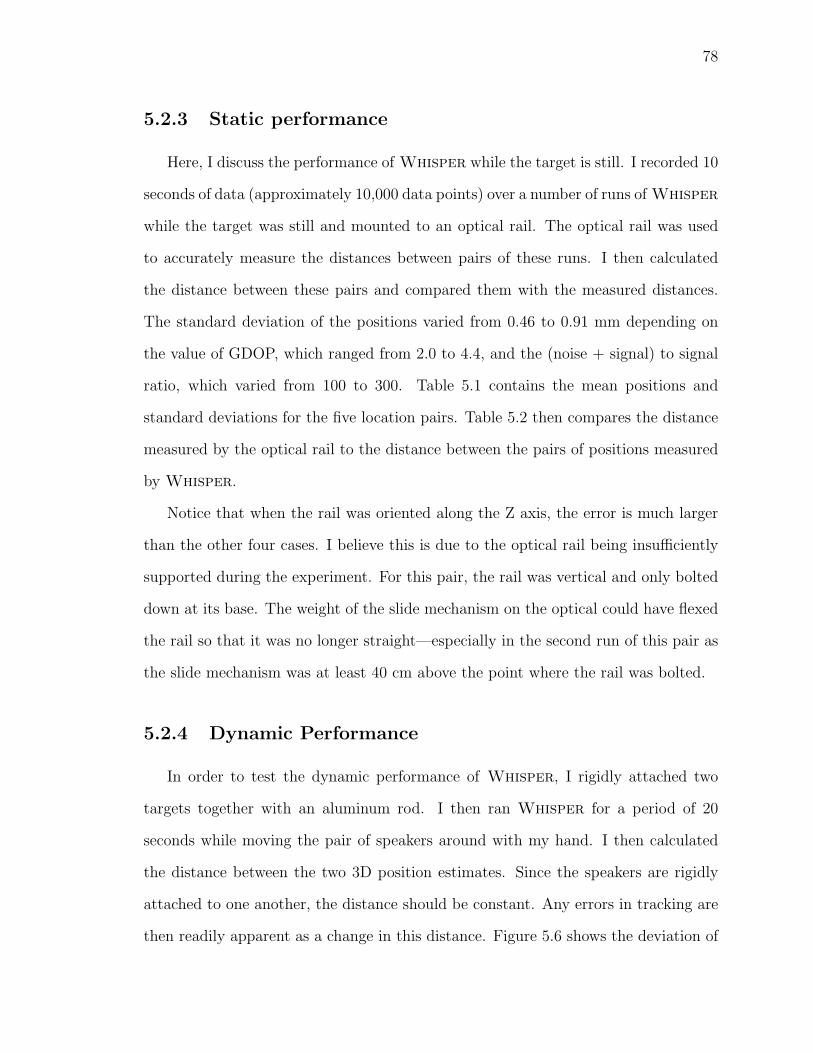
78
5.2.3 Static performance
Here, I discuss the performance of Whisper while the target is still. I recorded 10
seconds of data (approximately 10,000 data points) over a number of runs of Whisper
while the target was still and mounted to an optical rail. The optical rail was used
to accurately measure the distances between pairs of these runs. I then calculated
the distance between these pairs and compared them with the measured distances.
The standard deviation of the positions varied from 0.46 to 0.91 mm depending on
the value of GDOP, which ranged from 2.0 to 4.4, and the (noise + signal) to signal
ratio, which varied from 100 to 300. Table 5.1 contains the mean positions and
standard deviations for the five location pairs. Table 5.2 then compares the distance
measured by the optical rail to the distance between the pairs of positions measured
by Whisper.
Notice that when the rail was oriented along the Z axis, the error is much larger
than the other four cases. I believe this is due to the optical rail being insufficiently
supported during the experiment. For this pair, the rail was vertical and only bolted
down at its base. The weight of the slide mechanism on the optical could have flexed
the rail so that it was no longer straight—especially in the second run of this pair as
the slide mechanism was at least 40 cm above the point where the rail was bolted.
5.2.4 Dynamic Performance
In order to test the dynamic performance of Whisper, I rigidly attached two
targets together with an aluminum rod. I then ran Whisper for a period of 20
seconds while moving the pair of speakers around with my hand. I then calculated
the distance between the two 3D position estimates. Since the speakers are rigidly
attached to one another, the distance should be constant. Any errors in tracking are
then readily apparent as a change in this distance. Figure 5.6 shows the deviation of

79
Pair Mean Position Standard DeviationNumber X (cm) Y (cm) Z (cm) (cm)
1 28.85 17.51 -23.84 0.05058.86 17.54 -23.88 0.053
2 29.33 01.52 -21.29 0.04828.97 31.59 -20.91 0.091
3 46.51 7.33 9.17 0.07046.70 7.62 -21.09 0.046
4 19.26 11.54 -12.57 0.05543.87 26.52 -4.09 0.055
5 17.67 21.60 -13.40 0.06239.82 2.98 -5.27 0.060
Table 5.1: Mean position estimates for 10 Whisper runs while the target remainedat a fixed location on an optical rail. The rail was used to measure the distancebetween pairs of these runs.
Pair Rail Measured Rail Whisper EstimatedNumber Orientation Distance (cm) Distance (cm)
1 X 30.0 ± 0.1 30.002 Y 30.0 ± 0.1 30.073 Z 30.0 ± 0.1 30.264 Arbitrary 30.0 ± 0.1 30.025 Arbitrary 30.0 ± 0.1 30.06
Table 5.2: Comparison of distances measured using the optical rail to distances cal-culated between mean Whisper measurements.

80
0 2 4 6 8 10 12 14 16 18 20-10
-5
0
5
10
time (seconds)
devi
atio
n (m
m)
Deviation of interspeaker distance from the mean
Figure 5.6: Deviation of the inter-speaker distance over a tracking run of 20 seconds
this distance from the mean (202.7 mm) over the duration of the data collection. The
standard deviation of the deviation is 2.0 mm and the deviation is always less than 1
cm (approximately 5% of the inter-target distance). The velocities of the targets were
not insignificant during this test. In fact one of the targets exceeds the maximum
expected hand velocity of 3.0 m/s. The velocities of the two targets are shown in
Figure 5.7.
I wish to stress the difficulty of this test as the measure of a tracking device. It
has exposed the weaknesses of other tracking devices. It is especially convincing for
Whisper as the speaker geometry results in either a distance measurement along the
weakest axis with respect to GDOP or a higher angle from the main axis of the speaker
resulting in loss of signal because of transducer directionality. To further explain, the
two speakers are attached such that when they are directly facing the microphone
array, the distance between them is measured in a plane parallel to the plane of the
microphones. Measurements of the speaker locations in this plane (the Y and Z axes)
are the worst from the GDOP perspective. GDOP indicates that the distance from the

81
0 2 4 6 8 10 12 14 16 18 200.0
0.5
1.0
1.5
2.0
2.5
3.0
3.5
time (seconds )
spee
d (m
/s)
Target velocities for interspeaker measurements
Target 1 Target 2
Figure 5.7: Velocities of the two targets during the 20 second tracking run used toevaluate the dynamic performance of Whisper
microphone array (the X axis) is the most accurate for this geometry. However, when
the speakers are rotated such that the inter-speaker distance calculation is better from
a GDOP perspective, now the speakers are no longer directly facing the microphones
and so the signal is somewhat attenuated due to the loss of higher frequencies from
directionality.
5.2.5 Latency
The performance of an online tracking device involves more than the accuracy
of the position estimates. It also includes the latency of these estimates. A very
accurate measurement is not useful if it arrives after it is needed. It is especially
important for head-tracking data to have low latency as longer delays cause people to
feel like the world is “swimming” around them and can even lead to sickness. Latency
requirements for limb tracking are not so stringent, but it is still desirable to have
the lowest latency possible.

82
The upper bound on the latency of Whisper’s measurements is the sum of the
travel time of the acoustic signal, the delay from buffering incoming samples from
the microphone, the delay introduced by the correlation algorithm and the delay
introduced by the Kalman filter. The delay due to the travel time of the signal is
merely the range between speaker and microphone divided by the speed of sound. As
the maximum intended range for Whisper is approximately 1 meter, this produces a
delay of 3.4 ms. Whisper buffers incoming samples until there are k of them for the
next iteration. This introduces a latency of up to 100/fs seconds or 1 ms, although it is
more likely less than this. The delay through the correlation is approximately half the
length of the correlation window multiplied by the clock period (1/100000 s). Since
the longest window Whisper uses is 1000 samples, this yields a delay of 5 ms. Finally,
the delay through the Kalman filter changes as the noise on the measurements change.
The Kalman filter delay is measurable by inputting a step response in measurements
and calculating the 2% settling time of the Kalman filter’s response (the time it takes
for the response to get within 2% of its final value and remain there).
I measured the final three sources of latency as a group by feeding artificial sig-
nals into Whisper’s algorithm. I created an input signal by simply copying the
pseudonoise code. After one second of the copied code, I skipped one sample of the
code and continued for another second. This generates a one chip step in the delay
of the input signal. I can then measure the 2% settling time of the Kalman filter’s re-
sponse to this unit step input. I repeated this experiment twice to find the minimum
and maximum latencies, using the minimum and maximum observed noise to signal
ratios from the measurement noise data (see Figure 4.10). The results are shown in
Table 5.3. Note that the latency differs between the X dimension and the Y/Z di-
mensions due to the different values for the corresponding process noise. Including the

83
Noise/Signal Measurement Variance Latency LatencyRatio chips2 X (ms) Y,Z (ms)
6 0.01 14.8 16.8833 1.66 38.1 45.5
Table 5.3: Latency of Whisper algorithm for minimum and maximum noise to signalratios
time-of-flight delay between speaker and microphone, the total latency of Whisper
is in the range of 18.2 to 48.9 ms.
5.3 Tracking multiple targets
Whisper is not limited to tracking the position of only one target. In fact, one
of the great advantages of using direct sequence spread spectrum is the ability to use
CDMA to simultaneously track multiple targets. In order to track a 3D position,
ranges to at least three beacons must be calculated. At this point it becomes very
important to decide on the placement of the speakers and microphones. There are
benefits to both choices (microphones on targets or microphones at fixed locations).
Up to this point I have assumed the microphones are at fixed locations, as that
only requires one speaker (and thus one noise source) to track one target. Code
selection also becomes a concern at this point that I discuss in Section 5.3.2. Since
Whisper needs multiple speakers, no matter where the microphones are placed, the
pseudonoise codes need to have low cross-correlations. Even though CDMA gives us
the opportunity to add new speakers, there must be some limit to the number of
targets Whisper can track. I explore this limitation in this section as well.
84
5.3.1 Microphones Fixed or on Targets?
Assume that ranges are calculated to three fixed locations in order to calculate 3D
position. More beacons could be used to over-constrain the position, but this is the
minimum number necessary. Does the system function better with the microphones
at the fixed locations and the speaker on the targets or the other way around?
Whisper’s current implementation is capable of tracking two targets. This num-
ber is not larger primarily due to hardware constraints. The data acquisition board
Whisper uses has two analog outputs and 16 analog inputs. Given that ranges to
three fixed locations are necessary, it is obvious that Whisper must use the micro-
phones at the fixed locations and speakers on the targets for the current implemen-
tation. Without this restriction, is this still the right choice?
From the perspective of noise, microphones at fixed locations is the best choice for
two or fewer targets. This approach minimizes the number of speakers, and therefore,
the amount of acoustic noise produced by Whisper. When Whisper produces less
noise there is less noise in the environment, meaning less noise to interfere with
tracking and annoy users. Tracking three targets, it would not matter from the noise
perspective where the microphones are placed. For systems with greater than three
targets, it makes sense to have the speakers at fixed locations. Similar to the case
with less than three targets, this keeps the amount of acoustic noise to a minimum.
From the perspective of computation, it makes the most sense to mount the mi-
crophones to the targets. This is best seen by comparison with the GPS system. The
individual users of the GPS system have the receivers. This allows the system to
scale very elegantly. Since the users have the receivers, they are responsible for their
own computation. If the satellites had the receivers, they would have to perform all
the computation up in space, which would be impossible given the number of users
of GPS.

85
In Whisper the situation is not quite the same, but there are similar aspects.
When the microphones are at fixed locations then the computer to which the micro-
phones are connected must perform all the computations (or at least distribute the
raw data to multiple processors). However, given the small size of modern DSPs and
the growing integration of ADCs into DSPs, it would be fairly simple to provide a
processor for every microphone, conveniently located on the target.
It would be convenient if Whisper were a wireless system. As currently imple-
mented, there is a wire attaching the target back to the data acquisition board in
order to get the signal to the speakers. However, the speakers could be made wire-
less by attaching some very simple electronics that store the pseudonoise code and
continuously play it. An important issue in this scenario is that the speakers would
have to be synchronized with the microphones in some manner. One solution is to
add a fourth microphone and use the additional information to solve for the time
difference between the two parts of the system (just like GPS). Another solution is
to add a radio frequency receiver to the speaker and send a synchronization signal to
this receiver. The travel time of the radio signal would be insignificant.
Whisper’s latency is also affected by this decision. In Section 5.2.5 I indicated
that the travel time of the sound between the speaker and the microphones must be
considered in the latency measurement. This is because after the speaker moves, the
acoustic signal does not appear to the microphones to come from a different location
until it has had time to propagate the distance between the two. However, if the
mobile target is a microphone then any motion in the acoustic field created by the
(now stationary) speakers would be detectable instantaneously.
A final consideration is the size of the transducers. Speakers tend to be larger
than microphones. Given the intended usage of Whisper it makes sense to mount

86
the smaller of the two transducers to the targets (e.g., hands). This would be less
annoying to the user and also be less likely to interfere with his or her motion.
5.3.2 Selecting the Codes
With the addition of a second target, it is important to carefully select the code
used by each speaker (since there must be at least two speakers at this point). The
codes need to be as orthogonal as possible in the correlation sense. This means that
their autocorrelation is as impulse-like as possible, while their cross-correlations are
as low as possible at all correlation offsets.
Gold codes were designed for just such an instance. As mentioned previously,
their autocorrelation function is not as good as maximal length sequences, but their
cross-correlations have a guaranteed maximum value. Whisper doesn’t use binary
sequences, but instead uses uniform random numbers as it is easy to generate a
sequence of the desired length (as opposed to maximal length sequences that are
always 2n − 1 chips long).
Whisper uses uniform random numbers generated from a pseudo-random num-
ber generator built into Matlab. The use of maximal sequences, Gold codes, etc.
perform best when there is a constant length correlation window. The exceptional
characteristics of these sequences exist only when the correlation is performed over
the length of the entire sequence [Dixon 84]. We require the flexibility of variable
length correlation windows and so cannot make use of the optimal properties of these
codes.
In order to make sure that the Matlab random sequences perform at least as well
as the binary codes, I compared the autocorrelation and cross-correlation (between
different pseudonoise sequences) performance in simulation. One typical performance
measure used in the spread spectrum literature is the index of discrimination. This

87
is the difference between the magnitude of the autocorrelation at 0 delay and the
maximum autocorrelation value at any non-zero delay [Dixon 84]. The performance
measure I use for the simulations is what I will call the ratio of discrimination. This
is the ratio of the magnitude of the autocorrelation at 0 delay (the “peak”) to the
maximum autocorrelation at any non-zero delay or the maximum cross-correlation
at any delay. This has the added advantage of being independent of signal ampli-
tude, unlike the index of discrimination. The larger this ratio, the better the code is
performing.
I generate 1000 Matlab codes, each 100,000 samples long, and perform the correla-
tions using windows of 1000. This matches the parameters of the Whisper tracking
algorithm. The closest (in length) maximal length sequence is generated by a 17 bit
register and is therefore 131,071 samples in length. There are only a limited number
of maximal length sequences of this length so the results for maximal length sequences
are over a smaller set (I obtained 9 from [Dixon 84]).
Both autocorrelation and crosscorrelation of the Matlab random sequences com-
pare favorably to the maximal length sequences. The mean ratio of discrimination
for autocorrelation is 9.23 over a set of 1000 Matlab random sequences and 9.68 over
a set of 9 maximal length sequences. The values are similar for the crosscorrelation
of Matlab random sequences. Table 5.4 summarizes these results. As the crosscorre-
lation behavior of the Matlab random sequences is essentially identical to that of the
autocorrelation behavior, the use of multiple Matlab random sequences should not
degrade the system performance more than any other noise.
There are two additional factors that are important in the selection of a code for
Whisper. Even the longest window Whisper uses (1000 chips) does not allow for a
long enough signal to avoid the possibility of multipath interfering with the correlation
peak used for tracking. We need a code that is at least 15 meters long (approximately
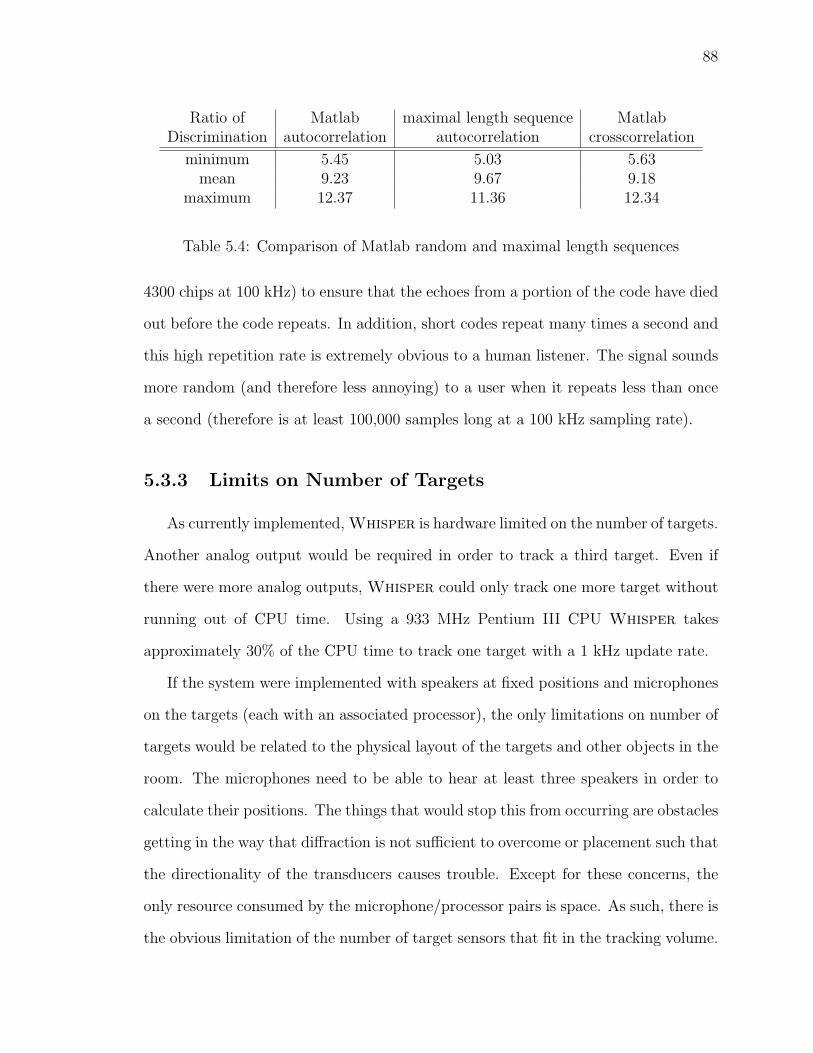
88
Ratio of Matlab maximal length sequence MatlabDiscrimination autocorrelation autocorrelation crosscorrelation
minimum 5.45 5.03 5.63mean 9.23 9.67 9.18
maximum 12.37 11.36 12.34
Table 5.4: Comparison of Matlab random and maximal length sequences
4300 chips at 100 kHz) to ensure that the echoes from a portion of the code have died
out before the code repeats. In addition, short codes repeat many times a second and
this high repetition rate is extremely obvious to a human listener. The signal sounds
more random (and therefore less annoying) to a user when it repeats less than once
a second (therefore is at least 100,000 samples long at a 100 kHz sampling rate).
5.3.3 Limits on Number of Targets
As currently implemented, Whisper is hardware limited on the number of targets.
Another analog output would be required in order to track a third target. Even if
there were more analog outputs, Whisper could only track one more target without
running out of CPU time. Using a 933 MHz Pentium III CPU Whisper takes
approximately 30% of the CPU time to track one target with a 1 kHz update rate.
If the system were implemented with speakers at fixed positions and microphones
on the targets (each with an associated processor), the only limitations on number of
targets would be related to the physical layout of the targets and other objects in the
room. The microphones need to be able to hear at least three speakers in order to
calculate their positions. The things that would stop this from occurring are obstacles
getting in the way that diffraction is not sufficient to overcome or placement such that
the directionality of the transducers causes trouble. Except for these concerns, the
only resource consumed by the microphone/processor pairs is space. As such, there is
the obvious limitation of the number of target sensors that fit in the tracking volume.

Chapter 6
Conclusions and Future Work
Whisper represents a novel approach to the problem of body-centered tracking
systems. Previous to this work, tracking systems either ignored the occlusion problem
or used magnetic or mechanical systems. Optical and acoustic systems used the first
approach, while the latter brought problems of its own such as low update rates, high
latency, heavily environment-dependent accuracy and the difficulty of donning and
doffing the tracking hardware.
The body-centered environment appears to be appropriate for the Whisper sys-
tem. The use of diffraction offers an approach to the occlusion problem. The limited
range between target and beacons helps to reduce past acoustic problems such as
temperature gradients and air currents. The addition of spread spectrum techniques
to acoustic tracking is obviously a win as it allows for fast update rates, simulta-
neous tracking of multiple targets and increased robustness to noise and multipath
interference.
6.1 Summary of results
Whisper is a successful prototype of an acoustic tracking device that shows
potential for use as a body-centered tracking system. Without occlusions, Whisper

90
reports the positions of two static targets with a standard deviation of 0.46 to 0.91
mm and 18 to 49 milliseconds of latency. In dynamic situations the standard deviation
could be as high as 2.0 mm.
Performance is better at shorter ranges due to the lower GDOP. Of course the
microphone array can be redesigned to produce low values of GDOP at whatever
location is desirable, limited only by the available locations for the microphones and
maximum range. Range is limited by the maximum power output of the speakers
and by error of up to 0.5% introduced by local atmospheric conditions.
Occlusions (even from small occluders) can cause Whisper to lose tracking of
the target if they are too close to the microphone or the speaker. This is due to
the increase in the length of the creeping wave. Longer creeping waves attenuate the
signal and result in a signal that is too weak for Whisper to track. Error introduced
by occlusions could be reduced even further by recognizing occluded situations and
reducing the length of the occluded range estimate. Since occlusions attenuate the
higher frequencies, there should be a characteristic change in the spectral content of
the incoming signal that would allow the detection of occlusion.
6.2 Other Applications
Besides the intended purpose of tracking hands and feet for virtual environment
purposes, Whisper could be applied to other tasks. Similar to the bench top system
currently implemented, Whisper could be used as a generic HCI device, much like
the ultrasonic 3D mice made by Logitech.
Another good use would be in the replacement of the ultrasonic beacons used by
Intersense’s Constellation system. This would increase the update rate and allow si-
multaneous range measurements from multiple beacons. Whisper would also provide
an excellent means of tracking the location of a building’s occupants with office-level
91
resolution. A worker would wear a small tag that played an extremely quiet acoustic
signal. Microphones in the office could use an extremely long correlation window to
detect this signal and use the knowledge to control things such as lighting and air
conditioning.
Whisper is not limited to tracking human targets. Although the system’s accu-
racy would be reduced over longer ranges, Whisper techniques could be used to allow
a robot, or any other electronic device for that matter, to determine its position within
a room, much like the system VTT Automation describes [VTT Automation 01], but
with the added benefit of Whisper’s occlusion tolerance and much higher update
rate. This could be especially useful to those who tend to lose their car keys—they
could ask the keys where they are.
6.3 Future Work
In order to make any device that functions in the real world robust, it must
be able to adapt to the current conditions in its environment. As this is such an
important topic, it will be discussed separately from the other opportunities that
exist for future work. Besides the adaptations that can be added to Whisper, there
are also a number of modifications that could improve the performance.
6.3.1 Adaptations
There is a tremendous amount of room to add adaptations to the Whisper system
to allow it to perform better. Some possibilities are:
• using auto gain control on the input. Currently, the microphone inputs have
fixed gain. The problem with this is that the gain must be set low enough so that
the ADCs are not overloaded when the range between speaker and microphone

92
is small. However, this means that not all the bits of the ADC are used when
the range is larger. Adding an auto gain control device should fix this issue.
Jason Stewart is currently working on this idea.
• allowing Whisper to use longer correlation windows. This would permit the
use of quieter signals and also would provide results with less noise when the
target is fairly still. It would however increase latency.
• changing output volume based on room noise level. Human beings adapt to
the current noise level in the room and “quiet” noises are only relatively so.
Whisper could monitor the current level of noise (not generated by Whisper)
and adapt its output volume to that level. To the human user, the volume
would appear to remain constant.
• dynamically changing the search window width (ns). Currently, this is constant,
but it could adapt to the Kalman filter’s estimate of its performance. If the
position estimates are less certain, it could expand its search space so that the
peak does not escape from the search space.
• more intelligent motion prediction for expanding the offset computation space
for computation reuse (better selection of nw). Whisper computes too much
currently as it makes the assumption that the target could take off at maximum
velocity in either direction at any point in time. Using a more realistic model
involving an estimate of maximum acceleration could reduce the computation
space even further.
• shaping the spectrum dynamically. When there is no occluder present, Whis-
per does not require low frequencies to operate. With the appropriate trans-
ducers, the signal could be moved into the ultrasonic region, making it inaudible

93
Microphones
Speakers
Figure 6.1: Conceptual drawing of a body-centered Whisper system. The mostdesirable configuration would probably have body-mounted speakers and microphonesattached to hands and other targets to be tracked.
to the user. This would also allow Whisper to play the signal more loudly in
the ultrasonic frequencies, resulting in better performance.
6.3.2 Modifications
The most important modification necessary is to produce a system that can be put
on a person and tested in a body-centered manner (Figure 6.1). The current benchtop
system is unsuitable to be worn. Given proof that Whisper works well in a body-
centered manner, it needs work to produce something that is small and wearable.
Related to this is the issue of the directionality of the speakers and microphones.
Once again, due to the wide range of motion a human is capable of, a target device
(speaker or microphone) on the hand experiences a wide range of orientations. One
solution to this is the use of arrays of devices on the hand. Whether these would be
merely multiple devices facing different ways with the same input/output signal or
something more sophisticated such as phased arrays must be determined.

94
If Whisper’s use is limited to the tracking of the body, the use of body kinematics
in the algorithm could improve the performance. As implemented, Whisper assumes
that the target could move in any direction with equal likelihood. However, the
structure of the human body limits the motions that are actually possible. These
factors could be included in the Kalman filter to improve its prediction capabilities.
Knowledge of the current state of the body could also be useful in the prediction
and detection of occlusions. If the system knows where the arms are, then it knows
whether or not a ranging pair should be occluded.
Although currently not used, Whisper could make use of the SCAAT Kalman
filter approach [Welch 97]. This approach is useful when measurements do not occur
at exactly the same time. In the algorithm description, I assume that the three
different range measurements all occur at exactly the same time. In reality, this
is not the case. The output of the three microphones are digitized by one ADC.
The ADC actually runs at three times the sampling rate desired (in Whisper’s
case this means it runs at 300 kHz to provide a 100 kHz sampling rate for each
microphone). Since there is just this one ADC, the microphone inputs must be
converted sequentially, and so at slightly different times. In the SCAAT Kalman
filter the measurement update does not provide the full information necessary to
determine all state variables. Instead, full information is provided over multiple filter
updates occurring at different points in time. The advantage is that the different
sampling times of the measurements are not ignored, but the predictor step must
be done more times in between measurements to update the filter’s prediction to
correspond to the time the measurement was made.
Currently the speakers and microphones are synchronized because they are at-
tached to the same data acquisition board. If they are to be separated (say to de-
velop a little device to mount to the target that consists of only a microphone and

95
a DSP chip), then another synchronization method is needed. This can be done by
calculating an additional range to a fourth fixed location and solving for the time
difference between the transmitter clock and the local clock (the same solution as
GPS uses). Similarly, an additional range measurement can be used to solve for the
speed of sound.
As I mentioned in Section 5.2.1, by using the speakers shown in Figure 5.4, it
could be possible to measure the speaker’s orientation in addition to the position. In
this case, the separation of the speaker into four separate sources at higher frequencies
becomes a benefit. One way to use this information is to modify the Kalman filter to
predict the shape of the correlation function instead of just using the position of the
largest peak in the search range. The difference between the predicted correlation
shape and the actual shape could then be used to update the state of the filter.
It is highly desirable to have a coarse to fine strategy for finding the correla-
tion peak. Currently, there is only the option of high-precision range measurements
that can only look in a very small search area. If there was some kind of multi-stage
approach that traded off precision for wider detection area, it could greatly aid Whis-
per. For instance, this allows for a re-acquisition process if the peak is lost. It also
allows the system to give up on really high-precision ranges when necessary (e.g., due
to noise or a bad occlusion scenario) and accept less accurate range measurements.
Whisper is essentially a spread spectrum communications system that is trans-
mitting no data. There is the possibility of transmitting data on the signal. However,
what data would be useful to transmit? One possibility is transmitting the location
of the fixed point to which a speaker is attached. This could allow the hopping of a
receiver from one reference point to another—much like the cells of cellular phones.
Multiple cells could use the same pseudonoise sequence as long as they are located
far enough apart from each other so that they do not interfere.

96
References
[Applewhite 94] Hugh L. Applewhite. A New Ultrasonic PositioningPrinciple Yielding Pseudo-Absolute Location. In VirtualReality Software and Technology: Proceedings of the VRST’94 Conference, pages 175–183, 1994.
[Arc Second 00] Arc Second. Vulcan 3D Measurement System. Productbrochure (see also http://www.arcsecond.com), 2000.
[Ascension 00] Ascension. MotionStar. Product brochure from AscensionTechnology Corporation (see alsohttp://www.ascension-tech.com), 2000.
[Atkeson 85] C. G. Atkeson & J. M. Hollerbach. Kinematic Features ofUnrestrained Vertical Arm Movements. Journal ofNeuroscience, vol. 5, pages 2318–2330, 1985.
[Bachman 01] E. R. Bachman, R. B. McGhee, X. Yun & M. J. Zyda.Inertial and Magnetic Posture Tracking for InsertingHumans into Networked Virtual Environments. In ACMSymposium on Virtual Reality Software and Technology(VRST), pages 9–16, Banff, Canada, 2001. ACM.
[Bhatnagar 93] Devesh Kumar Bhatnagar. Position Trackers for HeadMounted Display Systems: A Survey. Technical report,University of North Carolina at Chapel Hill, 1993.
[Bible 95] Steven R. Bible, Michael Zyda & Don Brutzman. UsingSpread-Spectrum Ranging Techniques for Position Trackingin a Virtual Environment. In Proceedings of the IEEEConference on Networked Realities ’95, Boston, MA, 1995.
[Bishop 84] Gary Bishop. Self-Tracker: A Smart Optical Sensor onSilicon. PhD thesis, University of North Carolina at ChapelHill Department of Computer Science, 1984.
[Boman 00] Mikael Boman, Asa Carlstrom, Jonas Ohlsson, RobertPedersen, Roonak Shakeri & Sedigh Sorush. WirelessDistance Measurement System. A class project report fromThe Royal Institute of Technology, department of Signals,Sensors and Systems in Sweden, May 2000.

97
[Brown 97] Robert Grover Brown & Patrick Y. C. Hwang. Introductionto Random Signals and Applied Kalman Filtering: withMATLAB Exercises and Solutions. John Wiley & Sons, Inc.,third edition, 1997.
[Charnwood 00] Charnwood. CODA mpx30. Product brochure fromCharnwood Dynamics Ltd, 2000.
[Dixon 84] Robert C. Dixon. Spread Spectrum Systems. John Wiley &Sons, second edition, 1984.
[Ferrin 91] Frank J. Ferrin. Survey of Helmet Tracking Technologies. InLarge-Screen-Projection, Avionic, and Helmet-MountedDisplays, volume 1456, pages 86–94. SPIE, 1991.
[Fleming 95] Robert Fleming & Cherie Kushner. Lowe-Power, Miniature,Distributed Position Location and Communication DevicesUsing Ultra-Wideband, Nonsinusoidal CommunicationTechnology. Technical report, AEther Wire and Location,Inc., 1995.
[Foxlin 98a] Eric Foxlin, Michael Harrington & Yury Altshuler. Miniature6-DOF Inertial System for Tracking HMDs. In Proceedingsof AeroSense 98 Conference on Helmet- and Head-MountedDisplays III, volume 3362, Orlando, FL, 1998. SPIE.
[Foxlin 98b] Eric Foxlin, Michael Harrington & George Pfeifer.ConstellationTM: A Wide-Range Wireless Motion-TrackingSystem for Augmented Reality and Virtual Set Applications.In SIGGRAPH 98 Conference Proceedings, AnnualConference Series, pages 371–378, 1998.
[Foxlin 00] Eric Foxlin & Michael Harrington. WearTrack: ASelf-Referenced Head and Hand Tracker for WearableComputers and Portable VR. In Proceedings of the FourthInternational Symposium on Wearable Computers. IEEE,2000.
[Girod 01] Lewis Girod & Deborah Estrin. Robust Range EstimationUsing Acoustic and Multimodal Sensing. In Proceedings ofthe IEEE/RSJ International Conference on IntelligentRobotics and Systems (IROS). IEEE/RSJ, 2001.
[Hightower 00] Jeffrey Hightower, Roy Want & Gaetano Borriello. SpotON:An Indoor 3D Location Sensing Technology Based on RFSignal Strength. UW CSE 00-02-02, University of
98
Washington, Department of Computer Science andEngineering, Seattle, WA, February 2000.
[Iltanen 98] Mika Iltanen, Heikki Kosola, Karri Palovuori & JukkaVanhala. Optical Positioning and Tracking System for aHead Mounted Display Based on Spread SpectrumTechnology. In Proceedings of the 2nd InternationalConference on Machine Automation (ICMA), pages 597–608,1998.
[Insko 01] Brent E. Insko. Passive Haptics Significantly EnhancesVirtual Environments. PhD thesis, University of NorthCarolina at Chapel Hill Department of Computer Science,2001.
[Kaplan 96] E. D. E. Kaplan. Understanding GPS Principles andApplications. Artech House, 1996.
[Keller 62] Joseph B. Keller. Geometrical Theory of Diffraction. Journalof the Optical Society of America, vol. 52, no. 2, pages116–130, February 1962.
[Maybeck 79] Peter S. Maybeck. Stochastic models, estimation, andcontrol, volume 141 of Mathematics in Science andEngineering. Academic Press, Inc., 1979.
[Measurand Inc. 00] Measurand Inc. ShapeTape. Product brochure fromMeasurand, Inc. Also available athttp://www.measurand.com/ as of July 1, 2002., 2000.
[Meta Motion 00] Meta Motion. Gypsy Motion Capture System. Productbrochure from Meta Motion, 2000.
[Meyer 92] Kenneth Meyer, Hugh L. Applewhite & Frank A. Biocca. ASurvey of Position Trackers. Presence, vol. 1, no. 2, pages173–200, 1992.
[Mine 97] Mark R. Mine. Exploiting Proprioception inVirtual-Environment Interaction. PhD thesis, University ofNorth Carolina at Chapel Hill Department of ComputerScience, 1997.
[Neubauer 68] Werner G. Neubauer. Experimental Measurement of“Creeping” Waves on Solid Aluminum Cylinders in WaterUsing Pulses. The Journal of the Acoustical Society ofAmerica, vol. 44, no. 61, pages 298–299, January 1968.

99
[Palovuori 00] Karri T. Palovuori, Jukka J Vanhala & Markku A.Kivikoski. Shadowtrack: A Novel Tracking System Based onSpread-Spectrum Spatio-Temporal Illumination. Presence:Teleoperators and Virtual Environments, vol. 9, no. 6, pages581–592, December 2000.
[Pierce 81] Allan D. Pierce. Acoustics: An Introduction to Its PhysicalPrinciples and Applications. McGraw-Hill Book Company,1981.
[Polhemus 00] Polhemus. FASTRAK. Product brouchure (see alsohttp://www.polhemus.com), 2000.
[Richards 00] Joseph L. Richards. A Spread Spectrum Sonar withNoise-Locked Loop-Based Entrainment. Master’s thesis,Massachusetts Institute of Technology, 2000.
[Roberts 66] Lawrence G. Roberts. The Lincoln Wand. In AFIPSConference Proceedings, 1966 Fall Joint ComputerConference, pages 223–227, 1966.
[Sorensen 89] Brett R. Sorensen, Max Donath, Guo-Ben Yang &Roland C. Starr. The Minnesota Scanner: A PrototypeSensor for Three-Dimensional Tracking of Moving BodySegments. IEEE Transactions on Robotics and Automation,vol. 5, no. 4, pages 499–509, 1989.
[Sutherland 68] Ivan E. Sutherland. A Head-Mounted Three DimensionalDisplay. In AFIPS Conference Proceedings, 1968 Fall JointConference, pages 757–764, 1968.
[US Navy 45] US Navy. Submarine Refrigeration and Air-ConditioningSystems. Bureau of Naval Personnel, December 1945.NavPers 16163. Available online athttp://www.maritime.org/fleetsub/ as of June 28, 2002.
[VTT Automation 01] VTT Automation. Ultrasonic Positioning. VTT Automationweb reference:http://www.vtt.fi/aut/kau/results/mobile/ultrasonic.htmlon November 20, 2001, 2001.
[Welch 95] Greg Welch & Gary Bishop. An Introduction to the KalmanFilter. Department of Computer Science TR95-041,University of North Carolina at Chapel Hill, Chapel Hill,NC, 1995.
100
[Welch 97] Greg Welch & Gary Bishop. SCAAT: Incremental Trackingwith Incomplete Information. In SIGGRAPH 97 ConferenceProceedings, Annual Conference Series, pages 333–344, 1997.
[Welch 01] Greg Welch, Gary Bishop, Leandra Vicci, StephenBrumback, Kurtis Keller & D’nardo Colucci.High-Performance Wide-Area Optical Tracking. Presence:Teleoperators and Virtual Environments, vol. 10, no. 1,pages 1–21, February 2001.