Sensors 2011, 11, 5661-5676; doi:10.3390/s110605661

sensors ISSN 1424-8220

www.mdpi.com/journal/sensors

Article

A Cabled Acoustic Telemetry System for Detecting and Tracking

Juvenile Salmon: Part 2. Three-Dimensional Tracking and

Passage Outcomes

Z. Daniel Deng 1,*, Mark A. Weiland

1, Tao Fu

1, Tom A. Seim

1, Brian L. LaMarche

1,

Eric Y. Choi 1, Thomas J. Carlson

1 and M. Brad Eppard

2

1 Pacific Northwest National Laboratory, P.O. Box 999, Richland, WA 99332, USA;

E-Mails: mark.weiland@pnl.gov (M.A.W.); tao.fu@pnnl.gov (T.F.);

Thomas.Seim@pnl.gov (T.A.S.); brian.lamarche@pnl.gov (B.L.L.); eric.choi@pnl.gov (E.Y.C.);

thomas.carlson@pnl.gov (T.J.C.) 2 U.S. Army Corps of Engineers, Portland District, P.O. Box 2946, Portland, OR 97208, USA;

E-Mail: matthew.b.eppard@usace.army.mil

* Author to whom correspondence should be addressed; E-Mail: zhiqun.deng@pnl.gov.

Received: 30 March 2011; in revised form: 20 May 2011 / Accepted: 23 May 2011 /

Published: 26 May 2011

Abstract: In Part 1 of this paper, we presented the engineering design and instrumentation

of the Juvenile Salmon Acoustic Telemetry System (JSATS) cabled system, a

nonproprietary sensing technology developed by the U.S. Army Corps of Engineers,

Portland District (Oregon, USA) to meet the needs for monitoring the survival of juvenile

salmonids through the hydroelectric facilities within the Federal Columbia River Power

System. Here in Part 2, we describe how the JSATS cabled system was employed as a

reference sensor network for detecting and tracking juvenile salmon. Time-of-arrival data

for valid detections on four hydrophones were used to solve for the three-dimensional (3D)

position of fish surgically implanted with JSATS acoustic transmitters. Validation tests

demonstrated high accuracy of 3D tracking up to 100 m upstream from the John Day Dam

spillway. The along-dam component, used for assigning the route of fish passage, had the

highest accuracy; the median errors ranged from 0.02 to 0.22 m, and root mean square

errors ranged from 0.07 to 0.56 m at distances up to 100 m. For the 2008 case study at John

Day Dam, the range for 3D tracking was more than 100 m upstream of the dam face where

hydrophones were deployed, and detection and tracking probabilities of fish tagged with

JSATS acoustic transmitters were higher than 98%. JSATS cabled systems have been

OPEN ACCESS

Sensors 2011, 11

5662

successfully deployed on several major dams to acquire information for salmon protection

and for development of more ―fish-friendly‖ hydroelectric facilities.

Keywords: acoustic tracking; underwater acoustic sensors; acoustic telemetry

1. Introduction

Despite advances in turbine design and dam operations, passage through turbines and spillways may

injure or kill downstream-migrating juvenile salmon [1-6]. The design and operation of more fish-friendly

hydroelectric facilities require reliable estimates of behavior, timing, and survival of the juvenile

salmonids as they migrate downstream [7-10]. Three-dimensional (3D) position estimates of fish surgically

implanted with acoustic transmitters can provide near-dam fish behavior and passage route-specific

survival rates. In addition, 3D position estimates provide near-dam vertical distribution data required

for other important turbine passage evaluation techniques such as blade-strike modeling [5,10].

Position estimation algorithms are used to locate a moving or stationary object using a reference

sensor network. Different signals and sensors are selected depending on applications. The Global

Positioning System (GPS) uses satellites to provide location estimates by measuring the time of arrival

(TOA) of radio signals [11,12]. An underwater acoustic tracking system provides reliable location

information of the sources by measuring TOA of acoustic pulses or calls from aquatic animals using a

network of underwater hydrophones or receivers with known locations [13,14]. However, the basic

principles underlying the two systems are the same except for different requirements for the TOA

measurement and geometric configuration of the sensor network.

Underwater acoustic tracking has become a common technology for studying and monitoring the

movement and behavior of aquatic animals [15,16]. Usually the absolute time required for the acoustic

signal to travel from the source location to the hydrophone is unknown, so time of arrival differences

(TOADs) are computed. For 3D source location estimation, a network of at least four hydrophones is

required so that four unknown variables—the reference TOA and the three coordinates of the source

location—can be solved using four quadratic (nonlinear) distance equations. When one component of

the source location is derived from another method, such as a pressure or depth sensor, the minimum

number of hydrophones required is then reduced to three. For two-dimensional (2D) source location, at

least three hydrophones are required because there are three unknown variables [17]. When there are

more hydrophones than the minimum requirement (i.e., with redundant hydrophones), this problem

becomes an over-determined system [17,18].

Many researchers have investigated this nonlinear problem, and several solvers have been

developed mathematically for different applications [13-29]. Watkins and Schevill [13] first described

the 3D position estimate problem using four hydrophones and developed a geometric method. Exact

solutions in various forms were also discussed by Fang [22], Wahlberg et al. [15], Spiesberger and

Fristrup [14], and Bucher and Misra [28]. However, an exact solution may not always be available due

to the nonlinearity of the four distance equations, errors in TOA or TOAD measurements, errors in

sound speed, and hydrophone location uncertainties. In such cases, it is necessary to consider it as an

optimization problem and estimate the source location by minimizing the errors.

Sensors 2011, 11

5663

The most common approximation employs iterative Taylor-series methods or variant Newton-Gaussian

methods, which linearize the equation using Taylor expansion and search for an approximate

numerical solution iteratively by minimizing the least-square error [20]. Foy [20] produced accurate

position estimates at reasonable signal-to-noise ratios (SNRs). However, the solution was very

sensitive to the initial conditions. Chan and Ho [25] introduced an intermediate variable to transform

the nonlinear distance equations into linear equations containing the new intermediate variable and the

original unknown variables. The authors then used an approximate realization of the maximum

likelihood estimator to find a noniterative and explicit solution and compared their results with those

from iterative Taylor-series methods. They found improved accuracy and efficiency at relatively high

SNR and small TOAD estimation errors. Wahlberg et al. [15] synthesized the methods proposed by

Watkins and Schevill [13] and Spiesberger and Fristrup [14] and developed a general mathematical

form for 2D and 3D systems and for both minimum number of receivers arrays and over-determined

arrays. Au and Herzing [16] successfully tracked dolphins using a star geometry in which a four-receiver

array was arranged as a symmetrical star. Chan et al. [30] improved their maximum likelihood (ML)

algorithms by starting from ML functions instead of linearizing the equations first, then derived a

closed-form approximate maximum likelihood algorithm. The authors demonstrated the new method’s

superior performance in 2D experiments.

In Part 1 of this paper [31], we presented the engineering design and instrumentation of the Juvenile

Salmon Acoustic Telemetry System (JSATS) cabled system, a nonproprietary sensing technology

developed by the U.S. Army Corps of Engineers, Portland District (OR, USA). All hydrophones are

synchronized to the universal GPS clock using a GPS card (Model GPS170 PCI, Meinberg Funkuhren

GmbH & Co. KG, Bad Pymont, Germany), resulting in detection time accuracy on a single system to

250 ns and across multiple systems to 500 ns. In addition, all JSATS components are required to pass

comprehensive acceptance and performance tests in a controlled environment before they are deployed

in the field [31,32]. Part 2 of this paper describes how the JSATS cabled system was employed and

evaluated in the field as a reference sensor network for detecting and tracking juvenile salmon.

The efficiencies of exact solvers are approximately 90% possibly because of the high accuracy of

clock management, hydrophone location survey, and improved performance of JSATS components.

Therefore, only the performance of exact solvers is presented in this paper.

2. Methods

2.1. Study Site

The John Day Dam, owned and operated by the U.S. Army Corps of Engineers, is located on the

Columbia River at river kilometer (rkm) 348, approximately 45 km east of the city of The Dalles,

Oregon (Figure 1). The dam consists of a powerhouse, spillway, and navigation lock, with fish ladders

at either end of the dam. The powerhouse is 602 m long and consists of 16 turbines with nameplate

capacity of 135 MW each and overload capacity of 155.3 MW each. The spillway has an overall length

of 374 m and contains 20 gates, each 15.2 m wide. Two prototype top-spill weirs (TSWs) were

installed at spillbays 15 and 16 during 2008.

Sensors 2011, 11

5664

Figure 1. Location of John Day Dam on the Columbia River at rkm 348.

2.2. Algorithm

Consider a transmitting source in a four-hydrophone array. Throughout this section, the boldface

letters indicate matrices or vectors. The source (S) and receiver (r) position vectors are defined as:

3,2,1,0),,(

),,(

T

T

izyx

sss

iiii

zyx

r

S (1)

The distance between transmitting source and hydrophones gives:

3,2,1,0,)()()()( 2

0

2222 iTtczsysxs iiziyix (2)

where c is the speed of sound, 0T is the time of travel from the source to the reference receiver

(receiver 0), and it is the TOAD between receiver i and the reference receiver. With it measured by the

common clock, the source position vector and 0T are the four unknowns.

Assuming the first receiver is located at the origin of the coordinate system and subtracting

Equation (2) for i = 0 from Equation (2) for i = 1, 2, and 3 [14,15], we obtain:

btSR 0

222 TcT (3)

where:

321

321

321

zzz

yyy

xxx

R ,

3

2

1

t

t

t

t ,

3

2

1

b

b

b

b , and 222

iii tcb r (3a)

Sensors 2011, 11

5665

From Equation (3):

)2

1( 0

2 TcTtbRS (4)

Substituting Equation (4) into 2

0

2TcT SS gives:

a

aqppT

2

0 (5)

214 cca TT tRRt , bRRt

TTcp 12

2

1, and bRRb

TTq 1

4

1 (5a)

Note that there are two possible solutions for 0T . If both are complex, there is no solution for the

given configuration and TOADs. A negative 0T is not possible. When there are two real non-negative

solutions, then both provide possible locations for the source. It is then necessary to identify which one

is physically possible. After 0T is determined, the source position (S) is obtained by Equation (4).

For this study, all hydrophones were installed at the dam face and looking upstream into the dam

forebay. In addition, the hydrophones were baffled with plastic cones lined with an anechoic material

to exclude loud noises emanating from structures downstream of the hydrophones. Therefore, the

physical solution from two real non-negative solutions would be upstream of the dam. When more

than four hydrophones detected the same transmitter message, the four with the optimum geometric

configuration for 3D tracking were selected using the criteria developed by Wahlberg et al. [15] and

Ehrenberg and Steig [33].

After the source location was obtained from 3D tracking, TOADs ( 321 ,, ttt ) and 0T were computed

using the estimated source location for the given hydrophone locations and speed of sound. Speed of

sound was calculated using an equation developed by Marczak [34]. The total time error was then

defined as:

2

00

2

33

2

22

2

11 )T-T()t-t()t-t()t-t( T

The detailed steps for 3D tracking and passage outcomes for this study are as follows:

1. Pool all detections of the same signal from different hydrophones. If more than four

hydrophones detect the same tag signal, select the four with the best geometric configuration

for 3D tracking. Compute the TOAD directly from detection time because all hydrophones are

synchronized to a universal GPS clock with accuracy within 0.5 µs.

2. Apply tracking solvers to estimate 3D locations and output solutions that are physical and

within the prespecified T (10 µs in this study).

3. Apply order 3 median filtering [35] to remove spurious locations and smooth fish tracks.

Assign a route of passage based on the along-dam component of the last tracked location.

4. Assign another set of passage routes based on the detections of the last two hydrophones at

different piers. For example, if the two hydrophones were at Pier 1 (numbering starting from

the Oregon side) and Pier 2, then the passage route would be assigned to the first turbine unit.

5. Compare the two sets of passage routes. If the difference for a fish is more than one bay, check

its trajectory and detection history manually.

Sensors 2011, 11

5666

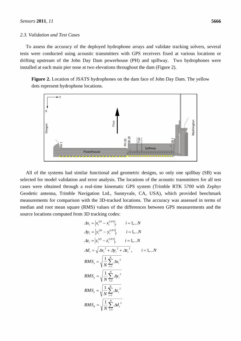
2.3. Validation and Test Cases

To assess the accuracy of the deployed hydrophone arrays and validate tracking solvers, several

tests were conducted using acoustic transmitters with GPS receivers fixed at various locations or

drifting upstream of the John Day Dam powerhouse (PH) and spillway. Two hydrophones were

installed at each main pier nose at two elevations throughout the dam (Figure 2).

Figure 2. Location of JSATS hydrophones on the dam face of John Day Dam. The yellow

dots represent hydrophone locations.

All of the systems had similar functional and geometric designs, so only one spillbay (SB) was

selected for model validation and error analysis. The locations of the acoustic transmitters for all test

cases were obtained through a real-time kinematic GPS system (Trimble RTK 5700 with Zephyr

Geodetic antenna, Trimble Navigation Ltd., Sunnyvale, CA, USA), which provided benchmark

measurements for comparison with the 3D-tracked locations. The accuracy was assessed in terms of

median and root mean square (RMS) values of the differences between GPS measurements and the

source locations computed from 3D tracking codes:

N

i

id

N

i

iz

N

i

iy

N

i

ix

iiii

GPS

i

D

ii

GPS

i

D

ii

GPS

i

D

ii

dN

RMS

zN

RMS

yN

RMS

xN

RMS

Nizyxd

Nizzz

Niyyy

Nixxx

1

2

1

2

1

2

1

2

222

3

3

3

1

1

1

1

,...1,

,...1,

,...1,

,...1,

Sensors 2011, 11

5667

where N was the number of estimated positions and x, y, and z were the three components in the

dam-face coordinate system. The dam-face coordinate system was defined as follows: the x-axis was

perpendicular to the dam and looking straight into the forebay; the y-axis was along the dam face from

the Oregon to the Washington side; and the z-axis was vertical, pointing upward.

The acoustic transmitters used in the validation tests had a ping rate of one pulse per second and a

source level of 155 dB relative to 1 μPa at 1 m. Transmitters were attached at different water depths to

a rope held steady by an anchor at the bottom. For the fixed-location tests, seven transmitters were

suspended at 1, 2, 3, 5, 10, 15, and 20 m below the water surface and held at various locations from

5 m to 100 m upstream of the dam in the forebay (Figure 3). Each fixed location test lasted

approximately 10 min, resulting in a typical sample size of 550 transmissions, given the 1-s pulse rate

repetition. For the drogue drift, six transmitters were held at 1, 2, 3, 5, 10, and 15 m below the water

surface. The GPS measurement point was about 1 m above the water surface. Because of the windy

conditions and underwater currents, the rope holding the transmitters was not always steady, resulting

in large uncertainties in transmitter locations in deep water. For this reason, only the transmitter held at

2 m below water surface was employed for the accuracy assessment, although all transmitters were

included for tracking efficiency analysis.

Figure 3. Error analysis test locations at John Day Dam spillway.

2.4. Field-Scale Application at John Day Dam

This case study involved a total of 2,445 yearling Chinook salmon (YC) and 2,448 steelhead (STH)

in Spring and in 2,483 subyearling Chinook salmon (SYC) in Summer passing through John Day Dam

during 2008. Median lengths of tagged fish for these downstream migrating YC, STH, and SYC were

158 mm, 217 mm, and 117 mm, respectively. All fish were surgically implanted [36] with JSATS

acoustic transmitters and passive integrated transponder (PIT) tags [37]. The size of the JSATS

acoustic transmitters differed from spring to summer due to technological advances in transmitter

design. In Spring, the transmitter mean weight was 0.485 g in air and 0.324 g in water, and transmitters

Spillbay9

Spillbay10

X(m)

Y(m

)

-20 0 20 40 60 80 100 120

740

760

780

800

South

MiddleNorth

Drogue Drift

Sensors 2011, 11

5668

were nominally 12.46 mm long, 5.30 mm wide, and 3.70 mm high. In Summer, the tag mean weight

was 0.425 g in air and 0.290 g in water. Summer tags averaged 12.04 mm long, 5.27 mm wide, and

3.74 mm high. The acoustic transmitters used in this study had a ping rate of one pulse every 3 s to

provide an expected transmitter life of at least 23 days.

Tagged YC and STH were released daily over a 29-day period in Spring (May 1 through May 29)

near Arlington, OR, USA at rkm 390 (42 km upstream of John Day Dam, at 0,600, 1,200, and

1,800 hours). Similarly, acoustic-tagged SYC were released in summer over a 29-day period (June 15

through July 13) in three release groups at Arlington, OR, USA (at 0,600, 1,200, and 2,100 hours).

To receive signals from tagged fish, we deployed shallow and deep JSATS cabled hydrophones on

the upstream face of John Day Dam with a total 21 systems and 84 hydrophones (dam-face array). We

also deployed and maintained autonomous node arrays [38] at river cross sections, including 2 km

upstream of John Day Dam (forebay array) and 9.4 km downstream of the dam (tailwater egress

array). The forebay array was used to create a virtual release for fish as they enter the forebay 2 km

upstream of the dam. The dam-face array was used to create a virtual release for fish known to have

passed John Day Dam and to estimate route of passage at the dam using 3D tracking and last-detection

data. The time of last detection by the dam-face array minus the time of first detection on the forebay

array provided an estimate of forebay residence time. The time of first detection by the John Day Dam

tailwater egress array minus the time of last detection on the dam-face array provided an estimate of

relative egress time. The PIT-tag detection system was used to provide the percentage of fish passing

the PH that were guided into the juvenile bypass facilities at John Day Dam.

Fish passage and behavior at the dam relative to the TSWs and two spill treatments (30% versus

40% spill out of total water discharge through the dam) were investigated using detections at the dam

face coupled with forebay hydrophone detections and acoustic tracking. Fish detections were classified

into ―arrival blocks‖ based on forebay array data and ―passage blocks‖ based on dam-face array data.

The blocks corresponded to areas of the dam, moving from south to north, as indicated in Figure 2: PH

turbine units 1–8, units 9–16, skeleton bays 17–20, SBs 17–20, TSW bays 15–16, and SBs 1–14.

Skeleton bays were included in arrival blocks but not in passage blocks because fish could not pass

there.

3. Results and Discussion

3.1. Validation Results

Tracking efficiency was evaluated as the number of successful 3D-tracked locations divided by the

number of transmissions. All transmitters had high tracking efficiencies at distances of 5 m to 100 m

from the dam face (Table 1). The transmitter attached to the rope at 20 m below the surface broke off

before the 5-m location test. Occasionally, there were low tracking efficiencies at a few locations; for

example, Transmitter 4 had an efficiency of 54.9% at 5 m and Transmitter 3 had an efficiency of

66.8% at 100 m. Tag 1 had lower efficiencies likely because of the multipath from the surface. These

infrequent dips in tracking efficiency were likely due to the fact that we could not control the

directivity of the transmitters during the tests.

Sensors 2011, 11

5669

Table 1. Tracking efficiency of JSATS cabled system at fixed locations.

Transmitter

index

Depth from

surface (m)

Tracking efficiency (%) at

5 m 15 m 30 m 50 m 75 m 100 m

1 1 87.0 89.0 88.6 86.8 69.3 49.9

2 2 93.9 95.5 88.8 96.7 87.4 80.3

3 3 92.1 89.1 90.4 93.0 86.7 66.8

4 5 54.9 99.6 99.1 98.9 94.8 86.8

5 10 98.8 99.3 99.6 98.8 98.2 96.5

6 15 84.6 99.5 98.6 99.1 98.3 97.7

7 20 N/A 89.1 98.7 98.5 99.1 95.8

Only the results of Transmitter 2 were selected for accuracy assessment. The median errors of the

x-component (the distance to the dam face) ranged from 0.06 to 0.55 m at distances up to 75 m and

ranged from 0.52 to 1.18 m at 100 m distance (Table 2).

Table 2. Median and RMS errors of the transmitter at 2 m below the water surface at SB 9,

John Day Dam spillway.

Location Distance

(m)

Median

(Δxi)

Median

(Δyi)

Median

(Δzi)

Median

(Δdi) RMSx RMSy RMSz RMSd

North

5 0.06 0.06 0.39 0.40 0.10 0.08 0.39 0.41

15 0.06 0.07 0.35 0.37 0.12 0.11 0.33 0.37

50 0.22 0.07 0.57 0.64 0.38 0.12 2.13 2.16

75 0.40 0.11 0.46 0.68 0.66 0.16 1.35 1.51

100 0.52 0.13 0.42 0.78 1.31 0.25 0.99 1.66

Middle

5 0.34 0.05 0.31 0.69 0.97 0.08 0.93 1.35

15 0.06 0.05 0.41 0.44 0.37 0.09 2.11 2.15

30 0.21 0.02 0.87 0.94 0.37 0.16 1.82 1.86

50 0.34 0.11 0.53 0.71 0.98 0.17 2.19 2.41

75 0.51 0.11 0.58 0.99 0.86 0.16 1.80 2.00

100 1.18 0.17 0.59 1.64 1.92 0.27 2.17 2.90

South

5 0.07 0.06 0.40 0.42 0.13 0.08 0.43 0.45

15 0.06 0.04 0.40 0.40 0.32 0.07 0.40 0.52

30 0.11 0.05 0.53 0.56 0.21 0.09 0.54 0.59

50 0.18 0.04 0.56 0.60 0.35 0.11 0.66 0.75

75 0.55 0.18 0.57 0.95 0.79 0.24 1.78 1.96

100 1.13 0.22 0.59 1.67 2.16 0.56 2.25 3.17

The RMS errors fell between 0.1 and 0.98 m for distances up to 75 m and between 1.31 and 2.16 at

100 m distance. Figure 4 contains interpolation of the Transmitter 2 results. The y-component, used for

the route assignment, had the highest accuracy among the three components. The median errors at SB

9 ranged from 0.02 to 0.22 m, and RMS errors ranged from 0.07 to 0.56 m at distances up to 100 m.

When the distance was less than 50 m, the median errors and RMS errors were within 0.07 and 0.16 m,

respectively. The z-component was in the vertical plane. At SB 9, the median errors of z-component

Sensors 2011, 11

5670

ranged from 0.31 to 0.87 m, and the RMS errors ranged from 0.33 to 2.25 m for all distances. For

absolute distances, the median errors were within 1 m for all distances except at the 100-m distance in

the south and middle section (1.64 m and 1.67 m, respectively). RMS errors of absolute distances

ranged from 0.37 to 3.17 m.

Figure 4. Contour plots of RMS errors of the transmitter at 2 m below the water surface,

John Day Dam spillway: (a) x; (b) y, (c) z.

For the drogue drift test, the overall tracking efficiency was 93.2% (Figure 5). The median errors in

x, y, z, and total distance were 0.20 m, 0.22 m, 0.38 m, and 0.52 m, respectively. xRMS , yRMS , zRMS ,

and dRMS were 0.49 m, 0.27 m, 0.95 m, and 1.10 m, respectively.

Both the median and RMS errors were computed from 3D-tracked positions that were slightly

smoothed by order 3 median filtering without removing outliers. If outliers were removed, or if

additional smoothing such as Kalman filtering algorithms were applied, the RMS errors could be

reduced significantly. In addition, windy conditions and underwater current probably caused

inaccuracies between GPS measurements and true transmitter locations, which would result in an

increase in RMS errors.

Sensors 2011, 11

5671

Figure 5. Comparison of GPS measurements and 3D-tracked positions at John Day Dam

spillway.

3.2. Case Study

Of the 7,376 tagged fish released upstream of John Day Dam, 7,118 (97%) were detected by the

autonomous receivers in the forebay. Of these 7,118 tagged fish, 7,067 (99%) were detected by the

cabled systems, with a median number of detections of 1,066 (Figure 6). Another 6,975 (98%) were

3D-tracked; the median number of tracking positions was 101 (Figure 7).

Figure 6. Number of detections by cabled systems at John Day Dam, 2008.

Number of Detections

Pe

rce

nt

of

De

tec

ted

Fis

h

0 500 1000 1500 20000%

10%

20%

30%

40%

Sensors 2011, 11

5672

Figure 7. Examples of 3D tracks at John Day Dam, 2008. Note that water surface is not plotted.

At least half of the tagged fish arriving upstream of the PH turbine units and skeleton bays moved

north to ultimately pass at the spillway, including the TSWs. This pattern was strongest for STH and

weakest for SYC. Tagged fish arriving upstream of the spillway, however, did not tend to move south

toward the PH (Figure 8). Specifically, for YC arriving in the forebay, 45% and 16% approached the

PH upstream of turbine units 1–16 and the skeleton bays, respectively, whereas 12% arrived at SBs

17–20, 5% at the TSWs, and 22% at SBs 1–14. Of the fish first arriving at the PH, nearly 60% moved

north and passed at the spillway, mostly at SBs 17–20 and the TSWs, closer to the PH. Conversely, 2%

of YC arriving at the spillway moved south and passed via the PH. The remaining 98% passed via the

spillway or TSWs.

For acoustic-tagged STH arriving in the forebay, 52% and 12% approached the PH upstream of

turbine units 1–16 and the skeleton bays, respectively. Arrivals at the spillway included about 9% at

SBs 17–20, 4% at the TSWs, and 23% at SBs 1–14. Nearly 66% of the STH that arrived at the PH

moved north and passed at the spillway, primarily at the TSWs. Similar to YC, the majority of STH

first approaching the spillway typically passed at SBs 1–14 or the TSWs; few STH arriving at the

spillway moved south and passed at the PH. Overall, a noticeable portion of STH moved toward the

TSWs, regardless of arrival block. For SYC, about 60% of those detected in the forebay arrived

upstream of the PH turbine units and the skeleton bays. About half of these fish moved north to

ultimately pass at the spillway, mostly at SBs 17–20 and the TSWs. Of the 25% of total SYC arriving

at units 9–16, more than one-half passed there or at units 1–8 and did not move north toward the

spillway.

Sensors 2011, 11

5673

Figure 8. Distribution of passage sections and first detection of yearling Chinook salmon

at John Day Dam, 2008.

Vertical distribution data were based on 3D tracking of individual acoustic-tagged fish. As smolts

moved from 75 m to within 10 m of the PH face, travel depths often decreased, but there was a sudden

increase to more than 20 m at a distance of less than 5 m from the PH. Note that PH piers on which

hydrophones were mounted do not extend more than about 1 m upstream of the PH face so that

sounding fish within 5 m of the dam face can be tracked moving down toward intake openings. The

turbine intake ceilings at John Day Dam are about 20 m deep. At the spillway, detection depths were

less than 5 m, regardless of distance upstream from the face of the spillway.

There was no difference in diel vertical distributions for PH- or spillway-passed YC. For STH,

vertical distribution was shallow for fish passed through the spillway; this pattern was especially

evident at the TSW. The last-detection depths at the PH were much deeper. Most SYC in the forebay

of the PH and skeleton bays traveled at depths between 5 and 11 m, while median depths of smolts

within 5 m of the PH or skeleton bays were between 20 and 25 m. As with YC and STH, the

last-detection depths for SYC were relatively shallow at the spillway. Notably, as SYC approached the

TSW, they migrated upward in the water column, but this trend was not evident for their approach at

non-TSW SBs.

4. Conclusions

Time-of-arrival information for valid detections on four hydrophones was used to solve for the 3D

position of fish surgically implanted with JSATS acoustic transmitters. Validation tests demonstrated

high accuracy of 3D tracking up to a 100-m distance at the John Day Dam spillway. The along-dam

component used for assigning the route of fish passage had the highest accuracy; the median errors

ranged from 0.02 to 0.22 m, and RMS errors ranged from 0.07 to 0.56 m at distances up to 100 m. For

the case study at John Day Dam during 2008, the range for 3D tracking was more than 100 m upstream

Sensors 2011, 11

5674

of the dam face, where hydrophones were deployed and detection and tracking probabilities were more

than 98%. JSATS cabled systems have been successfully deployed on several major dams to acquire

information for salmon protection and for development of more ―fish-friendly‖ hydroelectric facilities.

Acknowledgements

The work described in this article was funded by the U.S. Army Corps of Engineers, Portland

District. The study was conducted at Pacific Northwest National Laboratory (PNNL), operated in

Richland, Washington, by Battelle for the U.S. Department of Energy. The authors thank Robert

Wertheimer of the USACE and Derrek Faber, James Hughes, Mitchell Myjak, Geoff McMichael,

Gene Ploskey of PNNL for their help with this study. Numerous staff from the Pacific States Marine

Fisheries Commission and other PNNL staff from the Ecology Group, Hydrology Group, Marine

Sciences Laboratory, and Instrument Development Laboratory worked hard to develop and prove this

technology. Sonic Concepts Inc. provided innovative engineering, prototype development, and

production of transmitters and receiving equipment. Advanced Telemetry Systems set a new standard

for acoustic tag size and performance. Andrea Currie and Jayson Martinez of PNNL provided

comments and technical help preparing the manuscript. The authors are also grateful to the four

anonymous reviewers whose comments substantially improved the initial manuscript.

References

1. Cada, G.F. The Development of Advanced Hydroelectric Turbines to Improve Fish Passage

Survival. Fisheries 2001, 26, 14-23.

2. Odeh, M.; Sommers, G. New Design Concepts for Fish Friendly Turbines. Int. J. Hydropower

Dams 2000, 7, 64-71.

3. Neitzel, D.A.; Dauble, D.D.; Cada, G.F.; Richmond, M.C.; Guensch, G.R.; Mueller, R.P.;

Abernethy, C.S.; Amidan, B.G. Survival Estimates for Juvenile Fish Subjected to a

Laboratory-Generated Shear Environment. Trans. Am. Fish. Soc. 2004, 133, 447-454.

4. Deng, Z.; Guensch, G.R.; McKinstry, C.A.; Mueller, R.P.; Dauble, D.D.; Richmond, M.C.

Evaluation of Fish-Injury Mechanisms During Exposure to Turbulent Shear Flow. Can. J. Fish.

Aquat. Sci. 2005, 62, 1513-1522.

5. Deng, Z.Q.; Carlson, T.J.; Ploskey, G.R.; Richmond, M.C.; Dauble, D.D. Evaluation of

Blade-Strike Models for Estimating the Biological Performance of Kaplan Turbines. Ecol. Model.

2007, 208, 165-176, doi:10.1016/j.ecolmodel.2007.05.019.

6. Deng, Z.; Mueller, R.P.; Richmond, M.C.; Johnson, G.E. Injury and Mortality of Juvenile Salmon

Entrained in a Submerged Jet Entering Still Water. N. Am. J. Fish. Manage. 2010, 30, 623-628.

7. Nehlsen, W.; Williams, J.E.; Lichatowich, J.A. Pacific Salmon at the Crossroads: Stocks at Risk

from California, Oregon, Idaho, and Washington. Fisheries 1991, 16, 4-21.

8. Coutant, C.C.; Whitney, R.R. Fish Behavior in Relation to Passage Through Hydropower

Turbines: A Review. Trans. Am. Fish. Soc. 2000, 129, 351-380.

9. Deng, Z.; Carlson, T.J.; Duncan, J.P.; Richmond, M.C.; Dauble, D.D. Use of an Autonomous

Sensor to Evaluate the Biological Performance of the Advanced Turbine at Wanapum Dam.

J. Renew. Sustain. Energ. 2010, 2, 053104:1-053104:11, doi:10.1063/1.3501336.

Sensors 2011, 11

5675

10. Deng, Z.; Carlson, T.J.; Dauble, D.D.; Ploskey, G.R. Fish Passage Assessment of an Advanced

Hydropower Turbine and Conventional Turbine Using Blade-Strike Modeling. Energies 2011, 4,

57-67.

11. Parkinson, B.W.; Spilker, J.J., Jr.; Axelrad, P.; Enge, P. Global Positioning System: Theory and

Applications; American Institute of Aeronautics and Astronautics: Reston, VA, USA, 1996;

p. 793.

12. Misra, P.; Enge, P. Global Positioning System: Signals, Measurements, and Performance, 2nd ed.

Ganga-Jamuna Press: Lincoln, MA, USA, 2001; p. 569.

13. Watkins, W.A.; Schevill, W.E. Sound Source Location by Arrival-Times on a Non-Rigid

Three-Dimensional Hydrophone Array. Deep Sea Res. Part A 1972, 19, 691-706.

14. Spiesberger, J.L.; Fristrup, K.M. Passive Location of Calling Animals and Sensing of Their

Acoustic Environment Using Acoustic Tomography. Am. Nat. 1990, 135, 107-153.

15. Wahlberg, M.; Mohl, B.; Madsen, P.T. Estimating Source Position Accuracy of a Large-Aperture

Hydrophone Array for Bioacoustics. J. Acoust. Soc. Am. 2001, 109, 397-406.

16. Au, W.W.L.; Herzing, D.L. Echolocation of Wild Atlantic Spotted dolphin (Stenella frontalis).

J. Acoust. Soc. Am. 2003, 113, 598-604.

17. Drake, S.; Dogancay, K. Geolocation by Time Difference of Arrival Using Hyperbolic

Asymptotes. In Proceedings of 2004 IEEE International Conference on Acoustics, Speech, and

Signal Processing, Montreal, QC, Canada, 17–21 May 2004.

18. Friedlander, B. A Passive Localization Algorithm and Its Accuracy Analysis. IEEE J. Ocean.

Eng. 1987, 12, 234-245.

19. Huang, Y.; Benesty, J.; Elko, G.W.; Mersereau, R.M. Realtime Passive Source Localization: A

Practical Linear-Correction Least-Squares Approach. IEEE Trans. Speech Audio Process. 2001,

9, 943-956.

20. Foy, W.H. Position-Location Solutions by Taylor-Series Estimation. IEEE Trans. Aerosp.

Electron. Syst. 1976, AES-12, 187-194.

21. Tonieri, D.J. Statistical Theory of Passive Location Systems. IEEE Trans. Aerosp. Electron. Syst.

1984, AES-20, 183-198.

22. Fang, B.T. Simple Solutions for Hyperbolic and Related Position Fixes. IEEE Trans. Aerosp.

Electron. Syst. 1990, 26, 748-753.

23. Juell, J.-E.; Westerberg, H. An Ultrasonic Telemetric System for Automatic Positioning of

Individual Fish Used to Track Atlantic Salmon (Salmo salar L.) in a Sea Cage. Aquacult. Eng.

1993, 12, 1-18.

24. Axelrad, P.; Brown, R.G. GPS Navigation Algorithms. In Global Positioning System: Theory and

Applications; Parkinson, B.W., Spilker, J.J., Jr., Axelrad, P., Enge, P., Eds.; American Institute of

Aeronautics and Astronautics, Inc.: Reston, VA, USA, 1996; Volume 1, pp. 409-434.

25. Chan, Y.T.; Ho, K.C. A Simple and Efficient Estimator for Hyperbolic Location. IEEE Trans.

Signal Process. 1994, 42, 1905-1915.

26. Yarlagadda, R.; Ali, I.; Al-Dhahir, N.; Hershey, J. Geometric Dilution of Precision (GDOP):

Bounds and Properties; Technical Report 97CRD119; General Electric Research and

Development Center: Niskayuna, NY, USA, 1997.

Sensors 2011, 11

5676

27. Caffery, J.J., Jr. A New Approach to the Geometry of TOA Location. In Proceedings of Vehicular

Technology Conference Fall 2000—Bringing Global Mobility to the Network Age, Boston, MA,

USA, 24–28 September 2000; pp. 1943-1949.

28. Bucher, R.; Misra, D. A Synthesizable Low Power VHDL Model of the Exact Solution of a

Three-Dimensional Hyperbolic Positioning System. VLSI Des. 2002, 15, 507-510.

29. Cheung, K.W.; So, H.C.; Ma, W.-K.; Chan, Y.T. Least Squares Algorithms for Time-of-Arrival-

Based Mobile Location. IEEE Trans. Signal Process. 2004, 52, 1121-1128.

30. Chan, Y.T.; Hang, H.Y.C.; Ching, P.-C. Exact and Approximate Maximum Likelihood

Localization Algorithms. IEEE Trans. Vehic. Tech. 2006, 55, 10-16.

31. Weiland, M.A.; Deng, Z.; Seim, T.A.; LaMarche, B.L.; Choi, E.Y.; Fu, T.; Carlson, T.J.;

Thronas, A.I.; Eppard, B.M. A Cabled Acoustic Telemetry System for Detecting and Tracking

Juvenile Salmon. Part 1: Engineering Design and Instrumentation. Sensors 2011, 11, 5645-5660.

32. Deng, Z.; Weiland, M.; Carlson, T.; Eppard, M.B. Design and Instrumentation of a Measurement

and Calibration System for an Acoustic Telemetry System. Sensors 2010, 10, 3090-3099.

33. Ehrenberg, J.E.; Steig, T.W. A Method for Estimating the Position Accuracy of Acoustic Fish

Tags. ICES J. Mar. Sci. 2002, 59, 140-149.

34. Marczak, W. Water as a Standard in the Measurements of Speed of Sound in Liquids. J. Acoust.

Soc. Am. 1997, 102, 2776-2779.

35. Lim, J.S. Two-Dimensional Signal and Image Processing; Prentice Hall: Englewood Cliffs, NJ,

USA, 1990; pp. 469-476.

36. Deters, K.A.; Brown, R.S.; Carter, K.M.; Boyd, J.W.; Eppard, M.B.; Seaburg, A.G. Performance

Assessment of Suture Type, Water Temperature, and Surgeon Skill in Juvenile Chinook Salmon

Surgically Implanted with Acoustic Transmitters. Trans. Am. Fish. Soc. 2010, 139, 888-899.

37. Skalski, J.R.; Smith, S.G.; Iwamoto, R.N.; Williams, J.G.; Hoffman, A. Use of Passive Integrated

Transponder Tags to Estimate Survival of Migrant Juvenile Salmonids in the Snake and Columbia

Rivers. Can. J. Fish. Aquat. Sci. 1998, 55, 1484-1493.

38. McMichael, G.A.; Eppard, M.B.; Carlson, T.J.; Carter, J.A.; Ebberts, B.D.; Brown, R.S.;

Weiland, M.A.; Ploskey, G.R.; Harnish, R.A.; Deng, Z.D. The Juvenile Salmon Acoustic

Telemetry System: A New Tool. Fisheries 2010, 35, 9-22.

© 2011 by the authors; licensee MDPI, Basel, Switzerland. This article is an open access article

distributed under the terms and conditions of the Creative Commons Attribution license

(http://creativecommons.org/licenses/by/3.0/).