Object Tracking in a Stereo System Using Particle Filter of Computer Science and Engineering...
82
Department of Computer Science and Engineering University of Texas at Arlington Arlington, TX 76019 Object Tracking in a Stereo System Using Particle Filter Anup S. Sabbi [email protected] Technical Report CSE-2005-3 This report was also submitted as an M.S. thesis.
Transcript of Object Tracking in a Stereo System Using Particle Filter of Computer Science and Engineering...
Department of Computer Science and Engineering University of Texas at Arlington
Arlington, TX 76019
Object Tracking in a Stereo System Using Particle Filter
Anup S. Sabbi [email protected]
Technical Report CSE-2005-3
This report was also submitted as an M.S. thesis.

OBJECT TRACKING IN A STEREO SYSTEM
USING PARTICLE FILTER
The members of the Committee approve the master’sthesis of Anup S Sabbi
Manfred Huber
Supervising Professor
Farhad Kamangar
Gergely Zaruba

Copyright c© by Anup S Sabbi 2005
All Rights Reserved

OBJECT TRACKING IN A STEREO SYSTEM
USING PARTICLE FILTER
by
ANUP S SABBI
Presented to the Faculty of the Graduate School of
The University of Texas at Arlington in Partial Fulfillment
of the Requirements
for the Degree of
MASTER OF SCIENCE IN COMPUTER SCIENCE AND ENGINEERING
THE UNIVERSITY OF TEXAS AT ARLINGTON
May 2005

ACKNOWLEDGEMENTS
First and foremost, I would like to thank my dad Trinadh Rao, mom Ganga Naga-
mani and sister Naveena for their endless love, support and encouragement that made
all this possible.
I would like to offer special thanks to my supervising professor Dr. Manfred Huber
for his consistent help, support, and funding in this endeavor. I would also like to thank
Dr. Farhad Kamangar and Dr. Gergely Zaruba for being on my committee.
Last, but not the least, I would like to thank Ashok and Ajay for all those thought
provoking discussions. I extend my appreciation to my friends specially, Mahesh, Praveen,
Bharat, Prasanth, Sree and Greeshma for all the humor and fun.
April 22, 2005
iv
ABSTRACT
OBJECT TRACKING IN A STEREO SYSTEM
USING PARTICLE FILTER
Publication No.
Anup S Sabbi, M.S.
The University of Texas at Arlington, 2005
Supervising Professor: Manfred Huber
Tracking objects based on their visual features is of utmost interest in many do-
mains like robotics, manufacturing industry, surveillance and in smart environments.
This is a challenging problem because it has to deal with a huge amount of data that is
corrupted by noise. To deal with these issues, this thesis describes methods for tracking
objects in a stereo camera system using particle filters. A stereo system has to deal
with the stereo-correspondence problem to track objects in 3D. The proposed method
alleviates this problem by incorporating the stereo constraints into the particle filter.
To incorporate these constraints two possibilities were investigated. Firstly, two particle
sets, one for each of the left and right stereo image frames are maintained and a mapping
between the two sets is established by soft-stereo constraints. Secondly, the particles are
thrown into a three dimensional space and mapped back into the image frames to make
the observations. The observations are based on color, shape and texture of the object,
but the approach is not limited to using these features only.
v

In both of these approaches, Bayesian filtering provides the general framework for
the estimation of the state of the tracking system in the form of a probability density
function (pdf ) based on all the available observations. For a non-linear and non-Gaussian
model one of the challenges in this framework is to represent the pdf using finite com-
puter storage and to perform the integration efficiently when a new observation becomes
available. To overcome these difficulties Monte Carlo sampling-based techniques (particle
filtering) are used.
First observation or measurement models for the features of the objects are devel-
oped. Color histograms in the HSI color-space, edge density histograms for texture, and
shape similarity measures based on measurement lines are used to model the observations
and their likelihoods. Bhattacharyya distance is used as the distance metric for compar-
ing the target and candidate model histograms. These observations are then integrated
with the model of the system dynamics to obtain a posterior probability distribution for
the location of the object in the stereo images, using particle filters. Random Gaussian
displacements are used as the dynamics model of the individual particles. Location esti-
mates can be calculated from the obtained distribution.
The effectiveness of the approach is demonstrated by the experimental results. The
filter running two separate particle sets converges fast on the object, but the tracking er-
rors are higher than for a three-dimensional filter. The filter running in three-dimensional
space takes longer time to converge, but once it converges, the tracking is very effective
and the errors are lower than for the filter running with two separate sets of particles.
vi

TABLE OF CONTENTS
ACKNOWLEDGEMENTS . . . . . . . . . . . . . . . . . . . . . . . . . . . . . . iv
ABSTRACT . . . . . . . . . . . . . . . . . . . . . . . . . . . . . . . . . . . . . . v
LIST OF FIGURES . . . . . . . . . . . . . . . . . . . . . . . . . . . . . . . . . . ix
LIST OF TABLES . . . . . . . . . . . . . . . . . . . . . . . . . . . . . . . . . . . xi
Chapter
1. INTRODUCTION . . . . . . . . . . . . . . . . . . . . . . . . . . . . . . . . . 1
1.1 Overview . . . . . . . . . . . . . . . . . . . . . . . . . . . . . . . . . . . . 2
1.2 Application Domain . . . . . . . . . . . . . . . . . . . . . . . . . . . . . 3
2. PREVIOUS WORK . . . . . . . . . . . . . . . . . . . . . . . . . . . . . . . . 6
3. FILTERS . . . . . . . . . . . . . . . . . . . . . . . . . . . . . . . . . . . . . . 10
3.1 Bayesian Filter . . . . . . . . . . . . . . . . . . . . . . . . . . . . . . . . 10
3.2 Particle Filter . . . . . . . . . . . . . . . . . . . . . . . . . . . . . . . . . 13
4. FEATURES . . . . . . . . . . . . . . . . . . . . . . . . . . . . . . . . . . . . . 18
4.1 Color . . . . . . . . . . . . . . . . . . . . . . . . . . . . . . . . . . . . . . 19
4.2 Edges . . . . . . . . . . . . . . . . . . . . . . . . . . . . . . . . . . . . . 22
4.3 Texture . . . . . . . . . . . . . . . . . . . . . . . . . . . . . . . . . . . . 25
4.4 Shape . . . . . . . . . . . . . . . . . . . . . . . . . . . . . . . . . . . . . 27
5. PARTICLE FILTER MODELS . . . . . . . . . . . . . . . . . . . . . . . . . . 29
5.1 State Space Model for Particle Filter . . . . . . . . . . . . . . . . . . . . 29
5.2 Observation Model for Particle Filter . . . . . . . . . . . . . . . . . . . . 30
5.2.1 Color Likelihood Model . . . . . . . . . . . . . . . . . . . . . . . 30
5.2.2 Texture Likelihood Model . . . . . . . . . . . . . . . . . . . . . . 32
vii

5.2.3 Shape Likelihood Model . . . . . . . . . . . . . . . . . . . . . . . 33
5.3 Dynamics Model for the Particle Filter . . . . . . . . . . . . . . . . . . . 34
5.4 Soft Stereo Constraints . . . . . . . . . . . . . . . . . . . . . . . . . . . . 35
6. EXPERIMENTAL SETUP . . . . . . . . . . . . . . . . . . . . . . . . . . . . 38
6.1 Hardware . . . . . . . . . . . . . . . . . . . . . . . . . . . . . . . . . . . 38
6.2 Software . . . . . . . . . . . . . . . . . . . . . . . . . . . . . . . . . . . . 41
6.3 Pin-Hole Geometry . . . . . . . . . . . . . . . . . . . . . . . . . . . . . . 41
6.4 Location Estimates . . . . . . . . . . . . . . . . . . . . . . . . . . . . . . 42
6.4.1 Mean Estimate . . . . . . . . . . . . . . . . . . . . . . . . . . . . 42
6.4.2 Sum of Inverse Distances . . . . . . . . . . . . . . . . . . . . . . . 43
6.4.3 Density Estimate . . . . . . . . . . . . . . . . . . . . . . . . . . . 43
7. EXPERIMENTAL RESULTS . . . . . . . . . . . . . . . . . . . . . . . . . . . 44
7.1 Uncluttered Background . . . . . . . . . . . . . . . . . . . . . . . . . . . 44
7.2 Cluttered Background . . . . . . . . . . . . . . . . . . . . . . . . . . . . 53
7.3 Multiple Objects . . . . . . . . . . . . . . . . . . . . . . . . . . . . . . . 60
8. CONCLUSION AND FUTURE WORK . . . . . . . . . . . . . . . . . . . . . 64
8.1 Conclusions . . . . . . . . . . . . . . . . . . . . . . . . . . . . . . . . . . 64
8.2 Future Work . . . . . . . . . . . . . . . . . . . . . . . . . . . . . . . . . . 65
REFERENCES . . . . . . . . . . . . . . . . . . . . . . . . . . . . . . . . . . . . . 66
BIOGRAPHICAL STATEMENT . . . . . . . . . . . . . . . . . . . . . . . . . . . 70
viii

LIST OF FIGURES
Figure Page
3.1 SIS Particle Filter Algorithm . . . . . . . . . . . . . . . . . . . . . . . . . 15
3.2 Resampling Algorithm . . . . . . . . . . . . . . . . . . . . . . . . . . . . 16
3.3 Generic Particle Filter Algorithm . . . . . . . . . . . . . . . . . . . . . . 17
4.1 Color Cube for normalized RGB coordintes . . . . . . . . . . . . . . . . . 20
4.2 Hexacone representing colors in HSI . . . . . . . . . . . . . . . . . . . . . 21
4.3 Example histogram of an orange region . . . . . . . . . . . . . . . . . . . 21
4.4 One dimensional signal (sigmoid) . . . . . . . . . . . . . . . . . . . . . . 23
4.5 First derivative (Gaussian) . . . . . . . . . . . . . . . . . . . . . . . . . . 23
4.6 Second derivative . . . . . . . . . . . . . . . . . . . . . . . . . . . . . . . 24
4.7 Horizontal and Vertical Sobel masks . . . . . . . . . . . . . . . . . . . . . 24
4.8 Example texture histogram of checkered region . . . . . . . . . . . . . . . 26
4.9 Contour based shape filter showing the measurement lines and the edges . 28
5.1 Vergence Constraint . . . . . . . . . . . . . . . . . . . . . . . . . . . . . . 37
5.2 Epipolar Constraint (Gaussian) . . . . . . . . . . . . . . . . . . . . . . . 37
6.1 Stereo Head used for experiments . . . . . . . . . . . . . . . . . . . . . . 39
6.2 Range Resolution of the stereo head . . . . . . . . . . . . . . . . . . . . . 40
6.3 Pin-Hole camera goemetry . . . . . . . . . . . . . . . . . . . . . . . . . . 42
6.4 Example showing three different estimates . . . . . . . . . . . . . . . . . 43
7.1 Pendulum with uncluttered background . . . . . . . . . . . . . . . . . . . 46
7.2 Error estimates with different number of particles . . . . . . . . . . . . . 46
7.3 Error estimates with different number of particles . . . . . . . . . . . . . 47
ix

7.4 Error estimates with different number of particles . . . . . . . . . . . . . 47
7.5 Error in each frame using a SC filter with 1000 particles . . . . . . . . . . 48
7.6 Error in each frame using 3D filter with 2000 particles . . . . . . . . . . . 48
7.7 Error in each frame using a SC filter with 200 particles . . . . . . . . . . 49
7.8 Error in each frame using a SC filter with 400 particles . . . . . . . . . . 49
7.9 Error in each frame using a SC filter with 800 particles . . . . . . . . . . 50
7.10 Error in each frame using a SC filter with 1000 particles . . . . . . . . . . 50
7.11 Error in each frame using 3D filter with 200 particles . . . . . . . . . . . 51
7.12 Error in each frame using 3D filter with 400 particles . . . . . . . . . . . 51
7.13 Error in each frame using 3D filter with 2000 particles . . . . . . . . . . . 52
7.14 Error in each frame using 3D filter with 4000 particles . . . . . . . . . . . 52
7.15 Errors in each direction in each frame using SC filter . . . . . . . . . . . . 53
7.16 Error in direction in each frame using 3D filter . . . . . . . . . . . . . . . 54
7.17 Pendulum with cluttered background . . . . . . . . . . . . . . . . . . . . 54
7.18 Average Error in each frame using a SC filter with 200 particles . . . . . 55
7.19 Average Error in each frame using a SC filter with 400 particles . . . . . 55
7.20 Average Error in each frame using a SC filter with 800 particles . . . . . 56
7.21 Average Error in each frame using a SC filter with 1000 particles . . . . . 56
7.22 Average Error in each frame using a 3D filter with 200 particles . . . . . 57
7.23 Average Error in each frame using a 3D filter with 400 particles . . . . . 57
7.24 Average Error in each frame using a 3D filter with 800 particles . . . . . 58
7.25 Average Error in each frame using a 3D filter with 1000 particles . . . . . 58
7.26 Average Error in each frame using a 3D filter with 1500 particles . . . . . 59
7.27 Average Error in each frame using a 3D filter with 2000 particles . . . . . 59
7.28 Average Error in each frame using a 3D filter with 4000 particles . . . . . 60
x

LIST OF TABLES
Table Page
4.1 Simple objects and regions indicating texture . . . . . . . . . . . . . . . . 26
7.1 Frame Rates (frames/sec) . . . . . . . . . . . . . . . . . . . . . . . . . . . 44
7.2 Multiple-Object experiments . . . . . . . . . . . . . . . . . . . . . . . . . 61
xi

CHAPTER 1
INTRODUCTION
Computer vision deals with building systems to automate visual tasks which have
previously been performed by human beings, and to potentially improve their perfor-
mance. At a higher level of abstraction, most problems in computer vision can be cat-
egorized into two classes, (1) Object recognition, in other words to locate, distinguish
and classify a known object in images, (2) Object localization or tracking, which involves
determining the position of a known object in a sequence of image frames. The object
here can refer to a particular object or a general class of objects like chairs and tables.
This is an active area of research and no general algorithm has been proposed to solve
these problems. Instead, algorithms have been proposed to solve specific problems.
In the last decade research in computer vision gained a lot of momentum because
of the rapid increase in the computational power and the availability of cheap hardware.
Fundamental principles and techniques for pixel-level image processing were developed
reasonably well; the authors of [1] provide an overview of these techniques. Several com-
mercial vision systems have been successfully developed and deployed. Many techniques
have been proposed to track objects based on their visual cues. Most of the research
has concentrated on the problems of tracking using a single camera. But since depth
information is lost while tracking using a single image, tracking can be done only in two
dimensions. 3D information can be extracted from a single camera by taking multiple
images from different view points. Margaritis and Thrun [2] have used a single camera
mounted on a mobile robot to recognize and determine the location of objects in 3D
1
space using a grid-based probabilistic approach. Tracking objects in 3D space is still a
challenging problem, wether it be with a single camera or multiple cameras.
This thesis deals with the second type of problem in computer vision, and proposes
methods for object tracking in a stereo framework using particle filters. Tracking is done
based on the visual cues (features) of the object, including color, texture and shape.
Measurement likelihood models are developed for these features. A probabilistic approach
is taken for tracking in order to explicitly address the noise inherent in the images. The
Bayesian framework is used to track objects by estimating a probability density function
for the object’s location. Since the observation density could clearly be multi-modal in
this case the difficulty is to represent the pdf and to perform the integration whenever a
new observation becomes available. To overcome these difficulties Monte Carlo sampling
based techniques are used. Another problem is to incorporate the stereo constraints into
the particle filter. The two possibilities that are investigated are: (1) maintaining two sets
of particles, one for each of the stereo image frames, and establishing a mapping between
the two sets, (2)maintain particles in a three dimensional space and map them back into
the stereo image frames. For this approach it is assumed that the cameras are calibrated
and projective geometry is used to map the 3D locations onto the images. The dynamics
of the objects is modeled by gaussian random displacements. Similar approaches [3, 4, 5]
have been proposed recently to track objects in 3D based on color, but we have used a
novel approach of using two separate filters for each stereo image.
1.1 Overview
This section describes the organization of the content of this thesis. The next
section gives a brief description of the possible application domains of the proposed
method.
2

Chapter 2 provides an overview of the previous work in computer vision on tracking
objects. Chapter 3 gives a general introduction to filtering and then to Bayesian filters.
The Monte Carlo simulation of the bayesian filter often called particle filter is described
in detail. Chapter 4 describes the different features used in this thesis and the method-
ology used to extract them from the image frames. Observation models are needed to
statistically interpret the features desribed in Chapter 4, the models used are described
in Chapter 5. It also describes the state space model of the system and the dynamics
model. Chapter 6 describes the experimental setup used and the implementation details.
The experimental results are presented in Chapter 7. Chapter 8 gives the conclusions
and the future directions of the research.
1.2 Application Domain
With the availability of cheap and high resolution cameras, and the dramatic in-
crease in the information processing capabilities of computers, more and more visual
sensors are being hooked up to computers. Robotics, visual surveillance, manufacturing
and medicine are few domains where such hooks can be seen most commonly today. This
section gives a brief survey of the possible applications of computer vision in general and
the particular tracking techniques used in this thesis. This is not a comprehensive list
of all possible applications, a complete list of all possible applications of computer vision
and its current deployments in the industry would fill a volume in itself.
Robotics is a major field with endless possibilities for computer vision. Vision based
tracking systems in robotics have been used for various tasks ranging from robot soccer
to docking of space crafts. Robots must interact with the environment to perform various
tasks. Even more so for a mobile robot as it needs to negotiate obstacles and perform
3

its tasks. Therefore sensing mechanisms are required for these robots to track obstacles
and other moving objects. Tracking methods proposed here can be used on such robots
and also in developing systems to play games like ping-pong with human or other robot
opponents. They can also be used for applications in industry for component assembly,
inspection, binning different objects coming off an assembly line.
In Visual surveillance , as more and more cameras are being deployed to monitor
high security areas like airports, more people are required to watch the images from these
cameras. Since human observers have to deal with fatigue, the effectiveness of human
observation decreases over time. Therefore, an automatic warning system which alerts
on detection of suspicious activity is desirable. The proposed method can be used to
track objects in such places with less human intervention. Another similar application is
in automatic sports analysis by tracking players and the ball.
As automobiles are becoming more intelligent and the highways are getting more
crowded a computer vision system can be used to assist the driver. For example the
onboard vision system can look and track predefined sign boards and warn the driver
of an upcoming stop sign or reduced speed signs. Such a system can also be used for
automatic collision avoidance and pedestrian detection purposes. A vision based tracking
system can also be used on police cars to track particular vehicles based on the color of
the vehicle, license plates etc.
With the advent of smart homes, more and more advanced electronic devices are
being embedded into houses. Using and programming these devices can be confusing
and cumbersome for a child or an elderly person. The easiest way for them to deal with
these devices is by gestures. Vision-based tracking methods similar to the ones proposed
4

in this thesis can be used to track these gestures. A natural extension of such a gesture
recognition system is an imitation system. The easiest way to program a device is to
make it imitate its operator. Such visual systems can be used for behavioral analysis and
adapt the home environment to best suit the person’s preference. The system can get
feedback from the person by his gestures without him ever needing to program or even
press a single button.
5
CHAPTER 2
PREVIOUS WORK
Tracking in computer vision has attracted a lot of attention recently because of its
applications in real world problems, some of which were described in Chapter 1. Tracking
is a challenging problem because no sensor gives perfect measurements in all situations
wether it be cameras, laser range finders, sonars, infrared sensors, or RSSI readings from a
radio frequency device. For such systems tied down with uncertainty and noise, Bayesian
filters come as a rescue in representing and dealing with uncertainty. Not surprisingly
much of the research and solutions to tracking problems proposed were extensions of
Bayesian filtering techniques. This chapter gives a brief survey of the different Bayesian
filters used for tracking in computer vision and related fields.
The most widely used variant of the Bayesian filter is the Kalman filter [25]. Kalman
filters are optimal under the conditions that initial uncertainty is Gaussian and the ob-
servation model and system dynamics are linear in the state of the system. The like-
lihood distributions here are represented by a Gaussian N (µ, Σ), where µ is the distri-
bution’s mean and Σ is the d × d covariance matrix, assuming the systems state, x, is
d-dimensional. Since a Kalman filter can be implemented by simple matrix operations it
is computationally very efficient. However Kalman filters can only represent uni-modal
distributions. Spors and Rabenstein [6] have used Kalman filter to track human faces
using skin color and PCA based eye localization. Lee et al. [7] have used a Kalman filter
to track a toy train moving along 3D rails using a X-Y cartesian robot equipped with a
6
monocular camera placed orthogonal to the plane on which the tracks are placed.
The Kalman filter equations assume the system to be linear , but most systems are
not strictly linear. To overcome this problem an Extended Kalman filter (EKF) is often
used. In EKF, the idea is to linearize the measurement about the current estimate of
the state using first-order Taylor series expansions. Mikic et al. [8] have used Extended
Kalman filters to model and track human bodies in video streams.
EKF has potential drawbacks as it is difficult to implement and difficult to tune.
And if the time step intervals are not sufficiently small, this can lead to filter instability.
To address these issues with EKF, Unscented Kalman filters (UKF) are introduced [9].
Like in EKF, the state distribution in UKF is represented by a Gaussian Random Vari-
able (GRV), but it is represented using a minimal set of carefully chosen sample points.
The mean and covariance values of the GRV is captured by these sample points. When
these sample points are propagated through the non-linear system, the posterior mean
and covariance values are accurately captured up to the third order of the Taylor se-
ries expansion. Stenger et al. [10] have used UKF to track the 3D pose of a hand. A
comparison of UKF and EKF for tracking human hands and head for human-computer
interaction applications was performed in [11].
The Extended Kalman filter and the Unscented Kalman filter still have the limi-
tation of uni-modal distributions. Multihypothesis tracking techniques were introduced
to overcome this drawback. This tracking method represents the belief as a mixture
of Gaussians∑
i wiN (µi, Σi). Each Gaussian is tracked using a Kalman filter. Usually
a weight wi is associated with each Gaussian and in each update these weights are set
proportional to the likelihood of the sensor measurements. These Gaussian mixture tech-
7
niques are more computationally expensive and they require complicated heuristics to
determine the weights of each Gaussian in the mix.
Particle filters are Bayesian filters which can be easily implemented and do not
have the drawbacks of the Kalman filter methods. Particles filters have attracted a lot
of attention in tracking problems recently and have been used in numerous applications,
leading to a large amount of literature being available. So only the work that is closely
related to computer vision and this thesis is reviewed here. Particle filters were made
popular widely in computer vision by [12]. In this paper contour based observations were
used to track objects in clutter. The authors claim that in a clutter free environment,
Kalman filters could be used, but in the presence of clutter the Gaussian assumption in
KF’s cause the filter to perform poorly. Similar work on contour based tracking was done
in [13] to track human faces in images using an Unscented Particle Filter (UPF). It also
discussed tracking a speaker using audio sensors. Perez et al. [5] have taken advantage
of the data fusion properties of the particle filter to combine information from different
measurement sources. They have used a single camera and a stereo microphone pair for
tracking a speaker based on color, motion and sound cues. Spengler and Schiele [14] have
described a framework for multi-cue integration to increase the robustness of visual cue
based tracking systems. Shape based tracking systems were also described in [15, 16, 17].
Color-based particle filtering methods were described in [18, 19, 20]. The color
based models in the above papers have used similar histogram models that were used
in [21]. Very recently color-based particle filtering in multi-camera systems were inves-
tigated [3, 4]. The authors have claimed that they have not used any precise motion
models for tracking, and yet the tracking error estimates are under 5 cm for tracking
8

color blobs in a 8 cubic meter space.
Mobile robot localization is a related field in which particle filters for tracking were
first introduced. Dellaert et al. [22] have presented vision-based robot localization. They
have taken a novel approach to track the position of the camera platform rather than
tracking an object in the scene. Margaritis and Thrun [2] have used a single camera
mounted on a mobile robot to take several images of an object and estimate its 3D po-
sition.
Even though particle filters are not limited to Gaussian distributions, tracking mul-
tiple hypothesis is still a problem. Koller-Meier and Ade [23] have made an extension
to the particle filter algorithm so that multiple and newly appearing objects can also
be handled. Techniques similar to that of Mixture of Gaussians are used here. Another
multi-hypothesis tracking system for tracking people using a single static camera was de-
scribed in [24]. The idea here is to use a fast and robust observation model that reflects
the likelihood of differing number of objects present.
Particle filters were used in this thesis for tracking purposes. They are described
in more detail with experimental results in the following chapters.
9

CHAPTER 3
FILTERS
As opposed to the common notion of a filter as an electrical network, filter here
refers to a data processing algorithm. Filters are typically used to estimate an unknown
state of a system based on known measurements of the state. This can be visualized
as an estimation process, which has to deal with noisy measurements. Since the noise
is statistical in nature and can be modeled, this leads to stochastic estimation. This
chapter explains these estimation methods in detail.
3.1 Bayesian Filter
In all tracking problems it is required to estimate the state of the system as mea-
surements of the system , which most likely contain noise, become available. We need two
models to make inference in such systems, a system model and a measurement model.
The system model describes the evolution of the state of the system with time. The
measurement model encapsulates the noisy measurements made of the system. In the
Bayesian approach to dynamic state estimation a posterior probability density function
(pdf ) of the state is constructed based on all available information. A more detailed and
formal description is given below.
First, we need a mathematically tractable representation of the system, often called
a state-space model. In the case of tracking in images, state could be a 2D position in the
image, or it could be a multi-dimensional vector with 3D position and velocities in those
10

three directions. The state of the system at time t is represented by a random variable xt.
Assume that there are T frames of data to be processed, and at time t only data
from times 1, . . . t-1 are available. The measurements at time t are labeled Zt and will
contain a list of feature measurements as described in Chapter 4. The measurements up
to t are denoted Zt:
Zt = {Z1, · · ·Zt}.
Now the objective is to find the posterior density pt(xt|Zt) conditioned over all observa-
tions until time t, using Bayes’ formula:
pt(xt|Zt) = pt(xt|Zt,Zt−1)
=pt(Zt|xt,Zt−1)pt−1(xt|Zt−1)
pt(Zt|Zt−1)
(3.1)
Now, if pt(xt|xt−1) represents the system or dynamics model in the form of a probability
distribution, then Equation (3.1) can be expressed as:
pt(xt|Zt) =pt(Zt|xt,Zt−1)
∫xt−1
pt(xt|xt−1)pt−1(xt−1|Zt−1)dxt−1
pt(Zt|Zt−1)(3.2)
The complexity of computing such density increases exponentially over time, be-
cause of the accumulation of the measurements over time. To overcome this problem,
the Markov assumption is used to make Bayesian Filters computationally tractable. The
Markov assumption implies that observations are dependent only on the object’s current
location and its state at time t is dependent only on the previous state xt−1. States before
xt−1 provide no additional information. With the observation independence assumption
Equation (3.1) can be rewritten as:
pt(xt|Zt) =pt(Zt|xt,Zt−1)pt−1(xt|Zt−1)
pt(Zt)(3.3)
11
With the Markov assumption, it can be rewritten as:
pt(xt|Zt) =pt(Zt|xt)pt−1(xt|Zt−1)
pt(Zt)(3.4)
and Equation (3.2) can now be expressed as:
pt(xt|Zt) =pt(Zt|xt)
∫xt−1
pt(xt|xt−1)pt−1(xt−1|Zt−1)dxt−1
pt(Zt)(3.5)
p0(x0) is initialized with the priori distribution of the object’s locations in the im-
age. If no knowledge about the objects’ location is available, then a uniform distribution
can be used. Equation (3.5) gives the posterior distribution of the state of the system. As
new observations become available it needs to be recomputed to update the posterior pdf.
A Bayesian Filter that estimates Equation (3.5) is often called a Recursive Bayesian
Filter. And the equation is evaluated in two steps, namely prediction and update. In the
prediction step, the filter maps the previous posterior distribution pt−1(xt−1|Zt−1) into a
prediction density pt−1(xt|Zt−1) using:
pt−1(xt|Zt−1) =
∫xt−1
pt(xt|xt−1)pt−1(xt−1|Zt−1)dxt−1 (3.6)
The second step is the measurement update step. This step combines a new ob-
servation Zt with the prediction density pt−1(xt|Zt−1) above to get the desired posterior
density pt(xt|Zt):
pt(xt|Zt) =pt(Zt|xt)pt−1(xt|Zt−1)
pt(Zt)(3.7)
In the simplified case of the Kalman Filter [25], the observation density pt(Zt|xt) is
assumed Gaussian, and the dynamics is assumed to be linear. These assumptions make
the computation of Equation (3.5) simple. But these are highly unrealistic assumptions
12
in image-based tracking problems. Clearly the observation density here could be multi-
modal. Seeking an analytic solution to integrate Equation (3.5) over multi-dimensional
space is not tractable. So Monte Carlo-based integration methods are used to approx-
imate the solution. These are often called particle filters, which are discussed in the
following section.
3.2 Particle Filter
Particle filters have been used in a diverse range of applied sciences. The generality
and ease of implementation of particle filters make them ideal for many simulation and
signal processing problems. Particle Filtering is a technique for implementing a recursive
Bayesian filter by Monte Carlo simulations. The idea is to represent the pdf with a set
of random samples with associated weights and to compute estimates based on these
samples and weights. This section describes a basic particle filter in detail.
Particle filters are Sequential Monte Carlo (SMC) methods. Monte Carlo methods
are simulation-based methods which provide a convenient approach to computing the
posterior distributions. This section describes how these simulation methods can be used
to compute a pdf such as
pt(xt|Zt) =pt(Zt|xt)
∫xt−1
pt(xt|xt−1)pt−1(xt−1|Zt−1)dxt−1
pt(Zt)
which was developed in the previous section.
Variants of these methods are widely documented under the names Bootstrap Fil-
tering, Particle Filters, Interacting Particle Approximation, Condensation and Survival
of the fittest. Let Xt = {x1 . . .xt} be the sequence of states up to time t. Now, let
{X (i)t , π
(i)t }, i = 1 . . . N denote a Random Measure that characterizes the posterior pdf
13

p(Xt|Zt) where {X (i)t , i = 0 . . . N} is a set of support points with associated weights
{π(i)t , i = 1 . . . N}. The weights are normalized such that
∑i π
(i)t = 1. The posterior
distribution at time t is given by
p(Xt|Zt) ≈N∑
i=1
π(i)t δ(Xt −X (i)
t ) (3.8)
where δ is a Dirac-delta function with its mass located at 0.
Let xi ∼ r(x), i = 1 . . . N be the samples that are generated from proposal distri-
bution r(x), called an Importance density. The importance sampling technique is used to
choose the weights. This principle relies on the fact that, if p(x) is a probability density
from which it is difficult to draw samples, but for which q(x) can be evaluated, such that
q(x) ∝ p(x), then a weighted approximation to the density p(x) is given by
p(x) ≈N∑
i=1
πiδ(x− xi) (3.9)
where
πi ∝ q(xi)
r(xi)(3.10)
is the normalized weight of the ith particle.
If the samples, xit, were drawn from an importance density, r(Xt|Zt), then the
weights in Equation (3.9) are defined by Equation (3.10) to be
πit ∝
p(X it |Zt)
r(X it |Zt)
In the sequential case, at every iteration it is required to approximate p(Xt|Zt)
from p(Xt−1|Zt−1) with a new set of samples. If the importance density is chosen such
that it may be factorized as
r(Xt|Zt) = r(xt|Xt−1,Zt)r(Xt−1|Zt−1)
14

then samples X it ∼ r(Xt|Zt) can be obtained by adding each of the existing samples
X it−1 ∼ r(Xt−1|Zt−1) with a new state X i
t ∼ r(Xt|Zt). And the weight update equation
is given by
πit ∝ πi
t−1
p(Zt|xit)p(xi
t|X it )
r(xit|xi
t−1,Zt)(3.11)
An interested reader is referred to [26] for a derivation of the above relation. Now the
posterior density p(xt|Zt) can be approximated as
p(xt|Zt) ≈N∑
i=1
π(i)t δ(xt − x
(i)t ) (3.12)
as N →∞ the above approximation approaches the true posterior density. This method
of approximation is called Sequential importance sampling (SIS). The description is sum-
marized in the Figure 3.1 from [26].
[{xit, π
it}N
i−1] = SIS[{xit, π
it}N
i−1,Zt]FOR i = 1 : N
- Draw xit ∼ r(xt|xi
t−1,Zt)- Assign the particle a weight, πi
t, according to Equation (3.11)END FOR
Figure 3.1 SIS Particle Filter Algorithm.
There is an inherent degeneracy problem with the above SIS filter. After a few
iterations, most of the particles have negligible weights and significant computation is
done to update these particles which contribute little or nothing to the approximation
of p(xt|Zt). This is an undesirable effect in particle filters. Resampling is a method
used to reduce the effects of degeneracy. The principle behind resampling is to elimi-
nate the particles with insignificant weights and concentrate on particles with significant
weights. Resampling is accomplished by drawing N independent samples from the dis-
crete representation of p(xt|Zt) given in Equation (3.12) with replacement. An important
15
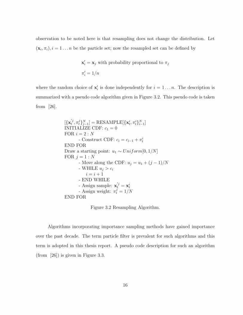
observation to be noted here is that resampling does not change the distribution. Let
(xi, πi), i = 1 . . . n be the particle set; now the resampled set can be defined by
x′i = xj with probability proportional to πj
π′i = 1/n
where the random choice of x′i is done independently for i = 1 . . . n. The description is
summarized with a pseudo code algorithm given in Figure 3.2. This pseudo code is taken
from [26].
[{x′jt , πj
t}Nj−1] = RESAMPLE[{xi
t, πit}N
i−1]INITIALIZE CDF: c1 = 0FOR i = 2 : N
- Construct CDF: ci = ci−1 + πit
END FORDraw a starting point: u1 ∼ Uniform[0, 1/N ]FOR j = 1 : N
- Move along the CDF: uj = u1 + (j − 1)/N- WHILE uj > ci
i = i + 1- END WHILE- Assign sample: x
′jt = xi
t
- Assign weight: πjt = 1/N
END FOR
Figure 3.2 Resampling Algorithm.
Algorithms incorporating importance sampling methods have gained importance
over the past decade. The term particle filter is prevalent for such algorithms and this
term is adopted in this thesis report. A pseudo code description for such an algorithm
(from [26]) is given in Figure 3.3.
16

FOR i = 1 : N- Draw xi
t ∼ r(xt|xit−1,Zt)
- Assign the particle a weight, πit, according to Equation (3.11)
END FORCalculate total weight: t = SUM [{πi
t}Ni=1]
FOR i = 1 : N- Normalize: πi
t = t−1πit
END FORINITIALIZE CDF: c1 = 0FOR i = 2 : N
- Construct CDF: ci = ci−1 + πit
END FORDraw a starting point: u1 ∼ Uniform[0, 1/N ]FOR j = 1 : N
- Move along the CDF: uj = u1 + (j − 1)/N- WHILE uj > ci
i = i + 1- END WHILE- Assign sample: x
′jt = xi
t
- Assign weight: πjt = 1/N
END FOR
Figure 3.3 Generic Particle Filter Algorithm.
17
CHAPTER 4
FEATURES
In-order to be able to track objects in images using particle filters, we need to define
observation likelihood models for these objects. Developing such models for a general
class of objects like chairs or tables is infeasible at this point because of the difficulty
in the understanding of the general notion of objects by a computer. So low level fea-
tures like color, texture and simple geometric shapes are used to describe objects. This
chapter describes the methodology used to obtain these low level observations, and their
likelihoods are discussed in Chapter 5. The proposed tracking methods are not limited
to these observations only, as new types of observations are developed, they can be easily
incorporated into the particle filter.
Sensors measure radiation reflected from objects usually resulting in two-dimensional
images. For example, a video camera records the intensity of light reflected from objects
in the scene, an infrared device produces a thermal image representing the temperature
of corresponding regions in the scene, and a laser range finder produces a range image
representing the distance of objects from the sensor. Intensity images formed by visible
light are most widely used in computer vision applications. These intensity images con-
tain a huge amount of data, so vision algorithms consider only a much smaller set of the
data, often called features. Color, texture and shape are the features used in this thesis,
and they are described in more detail in the following sections.
18

4.1 Color
Humans use color as one of the primary distinguishing feature of objects. For
example we might classify apples as green apples or red apples. Color can be used by
machines for the same purposes as by humans. One advantage of using color is the ability
to classify a single pixel of an image without complex spatial decision-making, in other
words with modest computation cost. Color based tracking methods have been proposed
in [18, 21, 20].
In digital computer systems color is often encoded by three bytes, each byte repre-
senting the amount of red, green and blue intensity. This type of encoding is called RGB
encoding. With such encoding, machines can distinguish between 16 million color codes,
but all these encodings may not represent differences that are significant in the real world.
Figure 4.1 shows the color cube in RGB space. In this representation any arbitrary color
in the visible spectrum can be obtained by combining the encoding of the three primary
colors, RGB. Since a byte is used for each R, G and B components, each can take a
value between 0 and 255. 0 representing the least intensity and 255 the highest. In this
setting pure red is encoded as (255,0,0), green as (0,255,0) and blue as (0,0,255). All the
other colors are encoded as a combination of intensity of these three colors, for example
yellow, which is a combination of red and green, is encoded as (255,255,0). Shades of
grey are combinations of the form (i,i,i), where 0 ≤ i ≤ 255. When i = 0 and 255, it
represents black and white, respectively. While the RGB color space is a straightforward
representation and many cameras output the color values in this format, the RGB values
change with the slightest change in the intensity of the image. This makes it harder to
model the observations in RGB space, so HSI color color space is used in this thesis.
19

��
��
��
-
6
��
��
��
��
�
��
�
Green
Blue
Red
Cyan
Magenta
Yellow
Black
White� Gray-scale Line
Figure 4.1 Color Cube for normalized RGB coordintes.
The Hue-Saturation-Intensity (HSI) color space decouples the chromatic informa-
tion from the shading effects. Here H and S together encode the chromaticity and I the
intensity. If we project the color cube in Figure 4.1 along its major diagonal (Gray-scale
line) we get a hexagon, which is represented by the base of an inverted hexacone as shown
in Figure 4.2. In the hexacone the vertical I axis is the major diagonal in the color cube.
Hue, H, is encoded as an angle between 0 and 2π relative to the red-axis, with pure red
at an angle of 0, pure green at 2π/3 and pure blue at 4π/3, with all angles represented in
radians. Saturation, S, models the purity of the color, with 1 modeling completely pure
color and 0 completely saturated. And intensity I, is a value between 0 and 1, with 0 at
the tip of the hexacone and 1 at the base. In HSI encoding, color black is represented as
(0,0,0) and is at the tip of the hexacone, while white is at the center of the base. Most of
the cameras output the images in RGB or YUV space, so a conversion to HSI is required,
a simple and fast algorithm is given in [27].
20

Figure 4.2 Hexacone representing colors in HSI.
A color feature filter is implemented here to output the bin number of a pixel based
on its HSI values. These bin numbers are used to build the histograms of the target
object and the candidate in the image, so that likelihood estimates can be obtained.
Color histograms of small regions typically of size 11× 11 are used in this thesis and an
example histogram of a region of an orange ball is shown in Figure 4.3. The methodology
used in evaluating the color histograms is described in the next chapter.
Figure 4.3 Example histogram of an orange region.
21
4.2 Edges
Edges in images generally characterize boundaries of objects, so they are of im-
mense interest in image processing and computer vision applications. Edges are the
areas in the image with sudden changes in the intensity. Edge detection filters out a lot
of useless information in the images, and yet preserves the structural properties of the
image. A good discussion of edges is presented in [28, 29, 30].
There are many methods to detect edges. In this thesis, for the sake of computa-
tional simplicity, gradient based edge detection is used. In the gradient based method
edges are detected by looking for the maximum and minimum in the first derivative of
the image. To visualize this, consider a one-dimensional signal as shown in Figure 4.4.
If we take the first derivative of the signal we get Figure 4.5, which clearly shows the
maximum at the center of the transition in the signal. If we look at the second deriva-
tive, Figure 4.6, the maximum in the first derivative corresponds to zero in the second
derivative. This method of finding zero crossings is often called the Laplacian method of
finding edges.
Extending this theory to two dimensions in images, Sobel operators can be used
to perform the spatial gradient measurement at each pixel location on the image. See
Figure 4.7 for the sobel operators. The operator Sx estimates the gradient in the x
direction and Sy estimates the gradient in the y direction. The magnitude of the gradient
is calculated using
|S| =√
S2x + S2
y (4.1)
This gradient value is compared with a threshold value τ to decide if the pixel at scrutiny
corresponds to an edge in the image.
22

- x
6f(x)
Figure 4.4 One dimensional signal (sigmoid).
- x
6f ′(x)
Figure 4.5 First derivative (Gaussian).
23

- x
6f ′′(x)
Figure 4.6 Second derivative.
Figure 4.7 Horizontal and Vertical Sobel masks.
24

4.3 Texture
Texture depends on the scale at which we view objects. The foliage of a tree has
a texture, but a single leaf occupying most of the image does not. This makes it hard to
define texture. There are two main approaches to define texture, structural and statisti-
cal. In the structural approach, texture is defined by a set of primitive texels arranged in
some regular or repeated relationship. Artificial textures can be defined by this structural
approach, but natural textures are more complicated and it is hard to define a canonical
set of texels for them. In the statistical approach, texture is described quantitatively
based on the arrangement of the intensities in a region. The statistical approach is less
intuitive but is computationally efficient.
Statistical texture measures are used in this thesis. The number of edges in a region
indicates the texture energy of that region. This is demonstrated in Table 4.1. If we look
closely at these images the checkered ball and the checkered board in the background in
the left image indicate regions with high edge density in the right image, when compared
to the rest of the image. As seen in the previous section, edge detection is easy to apply
and it is cheap if applied for small regions. In the experiments, regions of size 11 × 11
pixels are used. A gradient-based edge detector can be used to detect edges. The number
of edges per unit area can be used as a quantitative measure of the texture of the region.
Histograms can be obtained by discretizing the edge intensity values in the given region
into a fixed number of bins. Another way is to build the histogram with three bins, each
containing the number of horizontal, vertical and diagonal edges. The histograms thus
obtained can be compared to get a similarity measure. The texture feature filter outputs
the bin number of the pixel based on the edge intensity at the pixel location. These bin
numbers are used to build the histograms of the target and the candidate regions in the
image. An example texture histogram of a small region of a checkered ball is shown in
25

Table 4.1 Simple objects and regions indicating texture
Figure 4.8. The exact methodology used in evaluating the texture histograms and their
similarity measures is described in the next chapter.
Figure 4.8 Example texture histogram of checkered region.
26

4.4 Shape
We deal with thousands of objects every day. We know we can approach a vending
machine but not a speeding car for obvious reasons. Humans are very good at differ-
entiating objects. Unfortunately such a task is hard for a computer, partly because of
the difficulty in defining a generic shape signature for objects. This is apparent if we
try to give a generic definition for a simple object like a chair. Color and Texture are
not structural features. They provide no information about the shape or structure of
the objects in the image. This section describes the traditional methods used for finding
objects in images and the methods used in this thesis.
Traditionally, shape matching is done by template matching. Suppose we have a
template τ of the object of interest, and the goal is to find the instances of τ in the image
I. This can be done by placing τ at all the possible locations in the image and detect
the presence of the template at those locations by comparing the intensity values in the
template with the corresponding values in the image. The intensity values rarely match
exactly, so a similarity measure is required. Cross-correlation is the measure that is most
commonly used. The major limitations of template matching are that it is computation-
ally expensive and is not scale and rotation invariant. Template matching also fails in
case of partial occlusion.
Shapes can also be described by some primitive components and their spatial re-
lationship using a relational graph. These types of representations are invariant to most
2D transformations. Here the target and the candidate models are represented as graphs,
so graph matching algorithms can be used to get the similarity measures. Graph iso-
morphism can be used for matching in case of no occlusions and sub-graph isomorphism
can be used in case of occlusions, but graph isomorphism is an NP problem, and for any
27
reasonable object description the time required for matching can be prohibitive.
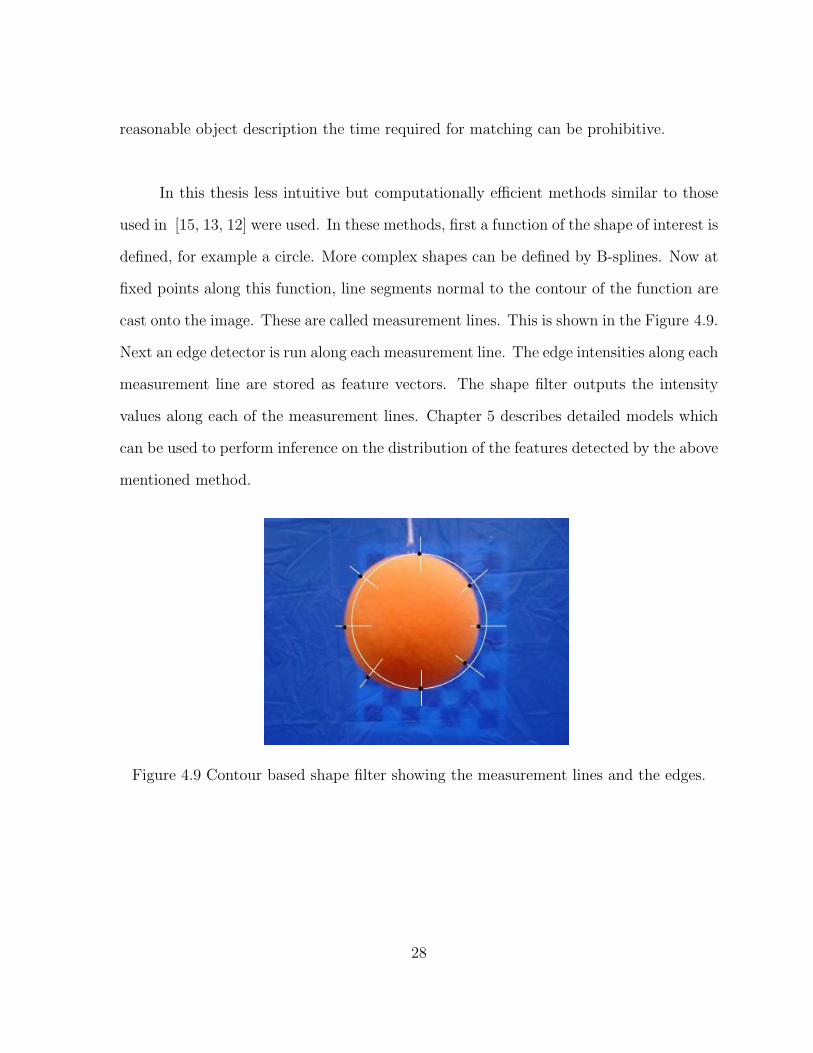
In this thesis less intuitive but computationally efficient methods similar to those
used in [15, 13, 12] were used. In these methods, first a function of the shape of interest is
defined, for example a circle. More complex shapes can be defined by B-splines. Now at
fixed points along this function, line segments normal to the contour of the function are
cast onto the image. These are called measurement lines. This is shown in the Figure 4.9.
Next an edge detector is run along each measurement line. The edge intensities along each
measurement line are stored as feature vectors. The shape filter outputs the intensity
values along each of the measurement lines. Chapter 5 describes detailed models which
can be used to perform inference on the distribution of the features detected by the above
mentioned method.
Figure 4.9 Contour based shape filter showing the measurement lines and the edges.
28

CHAPTER 5
PARTICLE FILTER MODELS
Previously, Chapter 3 described Bayesian filtering and particle filtering in generic
sense. In this chapter the particular models used for state-space representation, dynamic
models and the methodology used for estimating the observation likelihood in our particle
filter are discussed.
5.1 State Space Model for Particle Filter
In our case since we are tracking in a stereo environment, the additional challenge
is to incorporate the stereo constraints into the filter and be able to track in 3D. The first
possibility that was investigated is, maintaining two sets of particles, one for each of the
stereo image frames, and running a separate filter for both and mapping between the two
sets is achieved by enforcing soft constraints. These soft constraints enforce the epipolar
constraint and the constraint that objects can not be behind the camera. The second
possibility is to maintain the particles in a three dimensional space and map them back
into the image frames to make the observations at particular locations in the images. In
the case of two separate particles filters running in the two image frames, we can only
track objects in the image coordinates. For this case each sample state is defined as
x(L) = {x(L), y(L)}
x(R) = {x(R), y(R)}
where x(L),x(R) are the sample states corresponding to left and right images respectively
and x, y specify the location of the sample in image coordinates. This state representation
has two degrees of freedom, one in each direction of the image coordinates.
29
For the second case of tracking in 3D, the sample state is defined as
x = {x, y, z}
where x, y, z specify the location of the sample state in the 3D world coordinate system.
This representation has three degrees of freedom. In this representation the origin of the
coordinate system is fixed at the optical center of the left camera. These representations
are simple and straightforward. More complex and multi-dimensional state space models
could also be used because the filter can handle models that are much more complex.
For example, sample states could be defined as x = {x, y, z, x, y, z}, where x, y and z are
the velocities in x, y and z directions, respectively.
5.2 Observation Model for Particle Filter
An Observation model is required to statistically interpret the features described in
Chapter 4. Observation models are statistical models describing occurrences of features
in typical images. An observation model pt(Zt|xt) gives the likelihood of making the
observation Zt given that the object is at xt. The particular models used in this thesis
are described below.
5.2.1 Color Likelihood Model
In order to estimate the color likelihood models some reference color or target color
model is associated with the object of interest. This target model can now be compared
to the candidate regions in the image. The smaller the difference between the candidate
and target model, the higher the probability that the object of interest is located at the
corresponding region of the image. Histograms were used to define the models, similar to
the ones used in [21, 20, 18], and the likelihood is defined by the Bhattacharyya distance
between the two histograms.
30
Let {x∗i }i=1...n be the pixel locations of the sub-window of the image of the target
model for which the color histogram is being evaluated. The function hcolor(x∗i ) associates
to the pixel at location x∗i the index of the histogram bin depending on the color of the
pixel. If we discretize the histogram into m bins then hcolor : R2 7→ {1 . . . m}. In the
experiments, typically 8 × 8 × 4 bins were used to make the histogram less sensitive to
intensity variations.
Now the color distribution for the target model q = {qu}u=1...m is calculated as
qu =1
n
n∑i=1
δ[hcolor(x∗i )− u] (5.1)
where n is the number of pixels in the sub-window, δ is the Kronecker delta function,
and the normalization factor 1/n ensures that∑m
1 qu = 1.
Let {xi}i=1...nhbe the pixel locations of the sub-window of the target candidate
centered at y in the current image. The target candidates are the potential locations
of the regions of interest given by the locations of the particles. The color distribution
pu(y)of the target candidate can be calculated similarly as in Equation (5.1) as
pu(y) =1
nh
nh∑i=1
δ[hcolor(xi)− u] (5.2)
After computing the distributions of target model and the target candidate, we need
a similarity measure. The Bhattacharyya coefficient [31] is a popular measure which is
defined for the discrete densities q = {qu}u=1...m and p = {pu}u=1...m as
ρ[p, q] =m∑
u=1
√puqu (5.3)
The more similar the distributions are, the larger the value of ρ becomes. If the two
distributions are identical, we have ρ =∑m
u=1
√puqu =
∑mu=1 pu then we get ρ = 1. So
the range of ρ is [0,1]. A distance measure between the two distributions can now be
defined as
d =√
1− ρ[p, q] (5.4)
31
which is also called the Bhattacharyya distance. In the particle filter the samples (si, πi)
whose color distributions are similar to the target model are to be favored, so the weights
πi of the samples can be evaluated using
πi =1√2πσ
e− (1−ρ[psi ,q])
2ρ2 (5.5)
i.e., smaller Bhattacharyya distances correspond to larger weights.
5.2.2 Texture Likelihood Model
Texture likelihood models were developed along the same lines of the color mod-
els. A target model is associated with the object of interest. This target model is
now compared to the candidate regions in the image and the likelihood is defined by
the Bhattacharyya distance between the target histogram and the candidate histogram.
Again, let {x∗i }i=1...n be the pixel locations of the sub-window of the image of the tar-
get model for which the texture histogram is being evaluated. Typically 11 × 11 sized
sub-windows were used to construct the histograms. Now the function htex(x∗i ) asso-
ciates the pixel at location x∗i to the index of the histogram bin depending on the edge
intensity at the current pixel. Here, if the histogram were discretized into m bins, then
hcolor : R2 7→ {1 . . . m}. Similar to Equation (5.1) the texture histogram for the target
q = {qu}u=1...m is calculated as
qu =1
n
n∑i=1
δ[htex(x∗i )− u] (5.6)
where n is the number of pixels in the sub-window, δ is the Kronecker delta function,
and the normalization factor 1/n ensures that∑m
1 qu = 1.
32

Let {xi}i=1...nhbe the pixel locations of the sub-window of the target candidate
centered at y in the current image. The texture distribution pu(y)of the target candidate
can be calculated similarly as in Equation (5.6) as
pu(y) =1
nh
nh∑i=1
δ[htex(xi)− u] (5.7)
Now after computing target and candidate texture distributions, Bhattacharyya
coefficient is used as a similarity measure between the two histograms as given by
ρ[p, q] =m∑
u=1
√puqu
And the likelihood of texture observation can be evaluated using
πi =1√2πσ
e− (1−ρ[psi ,q])
2ρ2
5.2.3 Shape Likelihood Model
Objects with circular shapes are mainly considered in this thesis. If a shape obser-
vation is to be made at a location xt in the image, consider a circle centered at xt with
radius r. To make observations, K radial measurement lines are cast onto the contour of
this circle. These measurement lines are of fixed length and they extend a few pixels in
length on either side of the contour of the circle. The intersections (xk, yk), k = 1 . . . K
of each of the measurement lines with the circle are given by
xk = xt + rCosθk (5.8)
yk = yt + rSinθk (5.9)
The edge intensity values along the K measurement lines are used to model the
shape likelihood. Along these measurement lines the observation function hshape(xt) runs
a gradient-based edge detector to obtain the edge intensity values. In the presence of
clutter the measurements along each of the lines may have multiple-peaks signifying the
33
presence of multiple edge candidates. Let the number of peaks be S, then among these
S peaks at most one corresponds to the true contour of the object. Here we can define
S + 1 hypotheses, the first being hypothesis H0, which signifies that none of the peaks
correspond to the contour of the object. The rest of the hypotheses Hi, 1 ≤ i ≤ S mean
that the ith peak is associated with the contour of the object. Now the likelihood along
one measurement line can be given as
pk(zt|xt) = q0pk(zt|H0) +
S∑i=1
qipk(zt|Hi)
= q0U + NS∑
i=1
qiN ((xk, yk), σk)
(5.10)
such that, q0 +∑S
i=1 qi = 1. Where q0 is the prior probability of the hypothesis H0,
qi, i = 1 . . . S the edge intensity values at the peaks. N is the normalization factor, U
represents a uniform distribution and N (µ, σ) represents a Gaussian distribution.
If the measurement lines are far enough apart, it can be assumed that the feature
outputs along these measurement lines are statistically independent. Now the overall
likelihood of the K measurement lines is given by
p(zt|xt) =K∏
k=1
pk(zt|xt) (5.11)
5.3 Dynamics Model for the Particle Filter
The dynamics model describes how the state of the system changes at every time-
step. Since we are dealing with tracking objects in the real world, the most logical model
would be to incorporate the laws of Newtonian physics. Developing such a dynamics
model requires us to track the velocities and even accelerations in addition to the positions
of the objects, which increases the dimensions of the state of the system. With the
increase of dimensions the number of particles required to fill the multi-dimensional space
increases exponentially. To overcome these difficulties, Gaussian random displacements
34

are used here as a simplistic model of the dynamics of the particles in the particle filter.
The equations are given by
xt = xt−1 +N (0, σx) (5.12)
yt = yt−1 +N (0, σy) (5.13)
and in the case of the 3D filter, another equation is required for the motion in the z
direction, which is given by
zt = zt−1 +N (0, σz) (5.14)
The dynamics models do not favor motion in any particular direction, so σx, σy and σz
are all set to the same value α. The speed of the particles can be adjusted by changing
this value.
5.4 Soft Stereo Constraints
In the case of running two separate particle filters, one for each of the left and right
cameras, a mapping has to be introduced to incorporate the stereo constraints. Such a
mapping is not required for the 3D particle filter. This mapping is done using soft stereo
constraints which take into account the epipolar constraint and the vergence constraint.
The soft stereo constraints tie down the two particle sets and guides them so that the
violations of these constraints are restricted.
The epipolar geometry states that a point in the left image must lie on the epipolar
line in the right image corresponding to the particular point in the left and vice versa.
The orientation of this epipolar line is independent of the scene structure, and only de-
pends on the cameras’ internal parameters and the relative pose of the cameras. In other
words, epipolar geometry states that, an object present in the left image should appear
somewhere along a particular line(epipolar line) in the right image. And similarly, an
35

object present in the right image should appear along a particular line in the left image.
The vergence constraint imposes a restriction on the placement of the corresponding
points along the epipolar line. This constraint makes sure that impossible configurations
of correspondences are subdued, i.e., the configurations which state that the object the
camera is looking at is behind the camera.
The soft stereo constraint incorporates the above constraints by manipulating the
weights of the particles in both the particle sets. Assuming that the cameras are cali-
brated and the images rectified so that the epipolar lines are along the same line in both
the images and are parallel to the x-axis, each particles weight in the left particle set is
influenced by certain particle’s in the right set, given by
π(L)i = π
(L)i
n∑j=1
π(R)j f(x
(R)j − x
(L)i )N (y
(R)j − y
(L)i , σ) (5.15)
where π(L)i and π
(R)i are the weights of the particles in left and right sets, respectively. The
function f() is of the form shown in (Figure 5.1) and it spreads along the epipolar line,
in our case the x-axis of the image coordinate system. The function is placed along the
x-axis such that only the portions of the image along the epipolar line that do not violate
the vergence constraint fall inside the flattened peak of the curve. N () is a gaussian
distribution spread along an axis orthogonal to the epipolar line, as shown in (Figure
5.2). In this case it is spread along the y-axis. The value of σ is chosen such that it is
small enough to capture the epipolar constraint and large enough to allow the effects of
noise introduced by the dynamics model. The expression∑n
j=1 π(R)j f(x
(R)j −x
(L)i )N (y
(R)j −
y(L)i , σ) gives the weighted sum of all the particles in the right image, weighted according
to the two functions f() and N (). This weight is multiplied with the original weight of
36

the particle in the left set. The new weights are normalized to sum to 1. The weights of
the particles in the right particle set are updated similarly by the equation
π(R)i = π
(R)i
n∑j=1
π(L)j f(x
(L)j − x
(R)i )N (y
(L)j − y
(R)i , σ)
-x(R)(epipolar line)
6Inside edge of right image
Infinite distance point of x(L)i
f
Figure 5.1 Vergence Constraint.
- y(R)
6N
Figure 5.2 Epipolar Constraint (Gaussian).
37
CHAPTER 6
EXPERIMENTAL SETUP
This chapter describes the setup in which the experiments were carried out. All
experiments were carried out in as indoor laboratory environment. The sections below
explain in detail the hardware and software used and various assumptions made about
them.
6.1 Hardware
Any pair of cameras can be used for tracking using the proposed methods, provided
the intrinsic and the extrinsic parameters of the two cameras are known. The extrin-
sic parameters are the translation and rotation parameters between the two cameras.
Translation parameters are usually represented as [Tx, Ty, Tz], and rotation parameters
as [Rx, Ry, Rz]. Any calibration program can be used to estimate these values, in this
particular case they were estimated using SRI’s smallvcal program.
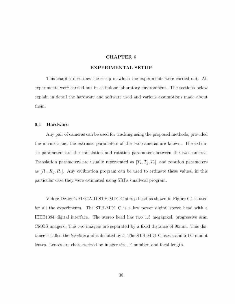
Videre Design’s MEGA-D STH-MD1 C stereo head as shown in Figure 6.1 is used
for all the experiments. The STH-MD1 C is a low power digital stereo head with a
IEEE1394 digital interface. The stereo head has two 1.3 megapixel, progressive scan
CMOS imagers. The two imagers are separated by a fixed distance of 90mm. This dis-
tance is called the baseline and is denoted by b. The STH-MD1 C uses standard C-mount
lenses. Lenses are characterized by imager size, F number, and focal length.
38
Figure 6.1 Stereo Head used for experiments.
The imager size is the largest size of imager that can be covered by the lens. For
the STH-MD1 C, a 2/3” or 1” lens can be used. For the experiments a 2/3” lens is used,
this caused a little bit of darkening at the edges of the image. F number is a measure of
the light gathering ability of a lens. The lower the F number, the better the lens will see
in low-illumination setting. The F number of the particular lenses used can be adjusted
manually between 1 and 1.8. The focal length is the distance from the lens virtual view
point to the imager, and it defines how large an angle the imager views through the lens.
Wide-angle lens have short focal length and telephoto lens have long focal length.
Another important factor for stereo cameras is the range resolution. Range reso-
lution is the minimum distance the stereo system can distinguish. Range resolution is
given by
∆r =r2
bf∆d
where b is the baseline, f if the focal length of the lens, r is the distance of the object from
the camera, and ∆d is the smallest disparity the stereo camera can detect. Figure 6.2
shows the range resolution of the stereo camera used, with f = 4.8mm, b = 90mm and
39

Figure 6.2 Range Resolution of the stereo head.
∆d = 3.0µm. It can be seen in this figure that the range resolution increases quadrati-
cally with the distance from the camera, experiments are designed to track objects that
are in the most effective range of the stereo camera.
The data from the STH-MD1 C is transfered to the host PC through a 1394 cable.
The 1394 interface can communicate at a maximum of 400MBps. Typically, 320 × 240
images are used for all experiments and the stereo camera could transfer up to 26 frames
per second at this resolution. A Dell Dimension desktop PC with a 1.8GHz Intel Pentium
4 CPU is used as Host PC. The stereo camera is connected to the PC using a OHCI
compliant 1394 PCI board.
40

6.2 Software
All the experiments were carried out on a system running Red Hat Linux 9.0 with
a 2.4.18-14 kernel. SRI’s Small Vision libraries are used to grab the images off of the
stereo camera.
6.3 Pin-Hole Geometry
In all the experiments, it is assumed that the cameras are calibrated and the images
rectified. With this assumption the left and right image planes are in the same plane, and
simple projective geometry can be used to calculate the 3D coordinates from the image
coordinates and vice versa. Figure 6.3 shows such a setup where L and R are pinhole
cameras with optical centers at L and R, respectively, and their optical axes parallel to
each other. Let f be the focal length of both cameras. The baseline is perpendicular to
the opitcal axes and the baseline distance is b. Let the world coordinate system (X,Y, Z)
be such that its X axis is along the baseline with its origin at the optical center of the
left camera. The optical axes lie in the XZ plane and the image planes are parallel to
the XY plane. In this setting, if the point P(x, y, z) is imaged as p1(x1, y1) and p2(x2, y2)
in the left and right image planes respectively, then the relationship between the world
and the image coordinates is given by
x =x1 × z
f(6.1)
y =y1 × z
f=
y2 × z
f(6.2)
z =b× f
(x1 − x2)(6.3)
41

- X
6
Z
��
��
��
��
@@
@@
@@
@@
L R
P(x, y, z)sp1(x1, y1)s p2(x2, y2)s
f b
Figure 6.3 Pin-Hole camera goemetry.
6.4 Location Estimates
The particle filter generates a posterior distribution of particles, which represents
the pdf. An example situation is shown in Figure 6.4, where the particle cloud is shown
by blue colored dots. Now, there are many possibilities to estimate the state of the
system from this distribution. The three types of estimates used here are as given below.
6.4.1 Mean Estimate
The mean estimate calculates the mean of the positions of all the particles. Mean
gives a very good estimate if the posterior distribution is unimodal and all the particles
form one ”blob”. But if there are multiple peaks in the distribution and there are two or
more blobs of particles, the mean can be a bad estimate, because it can provide a location
where there might not be a peak at all(or in the worst case, where the actual probability
of the object is 0). For instance in the example shown in Figure 6.4, the mean estimate
is shown as the red dot. In this particular case mean is a bad estimate, and it gives a
location where there is no orange object.
42

Figure 6.4 Example showing three different estimates.
6.4.2 Sum of Inverse Distances
This method computes the weight of each particle with respect to its distance from
all other particles. The distance from one particle to another is squared and inverted
to provide a weight with respect to the other particle. Such weights are computed with
respect to all other particles and these weights cumulatively determine the final weight
of the particle. The weights of all the particles used are computed and the one with the
maximum weight is designated the best estimate. In the example shown in Figure 6.4
this estimate is represented by a yellow dot.
6.4.3 Density Estimate
Similar to the above estimate, we compute a weight for each particle and the
particle with the highest weight is chosen as the best estimate. To compute the weight,
circular regions centered at each particle are assumed. The number of particles in each
such area is determined and used in the estimation of the weight. The distance from one
particle to another particle in the area is squared and inverted to provide a weight.In the
example shown in Figure 6.4 this estimate is represented by a green dot.
43
CHAPTER 7
EXPERIMENTAL RESULTS
In this chapter, various experiments are discussed and the results are presented.
To permit comparisons between filters with different particle numbers, pendulum exper-
iments conducted on image sequences recorded at constant frame rate of 75 frames per
second which for certain experiments with high particle numbers, may not be achievable
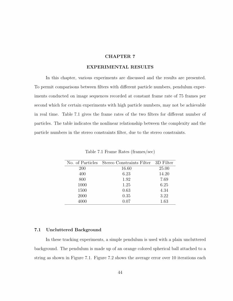
in real time. Table 7.1 gives the frame rates of the two filters for different number of
particles. The table indicates the nonlinear relationship between the complexity and the
particle numbers in the stereo constraints filter, due to the stereo constraints.
Table 7.1 Frame Rates (frames/sec)
No. of Particles Stereo Constraints Filter 3D Filter200 16.60 25.00400 6.23 14.20800 1.92 7.691000 1.25 6.251500 0.63 4.342000 0.35 3.224000 0.07 1.63
7.1 Uncluttered Background
In these tracking experiments, a simple pendulum is used with a plain uncluttered
background. The pendulum is made up of an orange colored spherical ball attached to a
string as shown in Figure 7.1. Figure 7.2 shows the average error over 10 iterations each
44
for different numbers of particles with a stereo constraints filter(blue curve) and a 3D
filter(purple curve). For the stereo constraints filter, the particle numbers indicated in
the figures are the number of particles in each set. By looking at the results in this figure,
the cumulative error in the 3D filter is higher than the stereo constraints filter. This is
because the 3D filter takes longer time to home in on the object. It can be observed here
that the precession of tracking increases with the increase in the number of particles.
And by looking at Figure 7.3 and Figure 7.4, which show the asymptotic error, i.e., the
error once the filter homes in on the object, it can be observed that the 3D filter tracks
reliably when compared to the stereo constraints filter. This is also evident by looking
at the results in Figure 7.5 and Figure 7.6, which show that the stereo constraints fil-
ter homes in on the object faster than the 3D filter, but the final estimation errors are
slightly higher, whereas the 3D filter takes more time to locate the object but once it
locates it, the error variance is low. This observation leads to the idea of using the stereo
constraints filter to coarse-localize and as the filter homes in on the object, the tracking
is switched to the 3D filter.
Figure 7.7, Figure 7.8, Figure 7.9 and Figure 7.10 show the errors in each frame
with different particle sets using a stereo constraints filter. As the number of particles
increases the precession increases. Figure 7.11, Figure 7.12, Figure 7.13 and Figure 7.14
show the errors in each frame with different particle sets using a 3D filter. Here also the
precision increases with the increase in the number of particles.
Figure 7.15 and Figure 7.16 show the errors in the individual x, y, and z coordinates
in each frame as the tracking process continues. Figure 7.15 shows the errors in the stereo
constraints filter running with 800 particles in each set, it can be seen here that the errors
in the z direction are slightly higher. Figure 7.16 shows the errors in the 3D filter with
45

Figure 7.1 Pendulum with uncluttered background.
Figure 7.2 Error estimates with different number of particles.
46

Figure 7.3 Error estimates with different number of particles.
Figure 7.4 Error estimates with different number of particles.
47

Figure 7.5 Error in each frame using a SC filter with 1000 particles.
Figure 7.6 Error in each frame using 3D filter with 2000 particles.
48

Figure 7.7 Error in each frame using a SC filter with 200 particles.
Figure 7.8 Error in each frame using a SC filter with 400 particles.
49
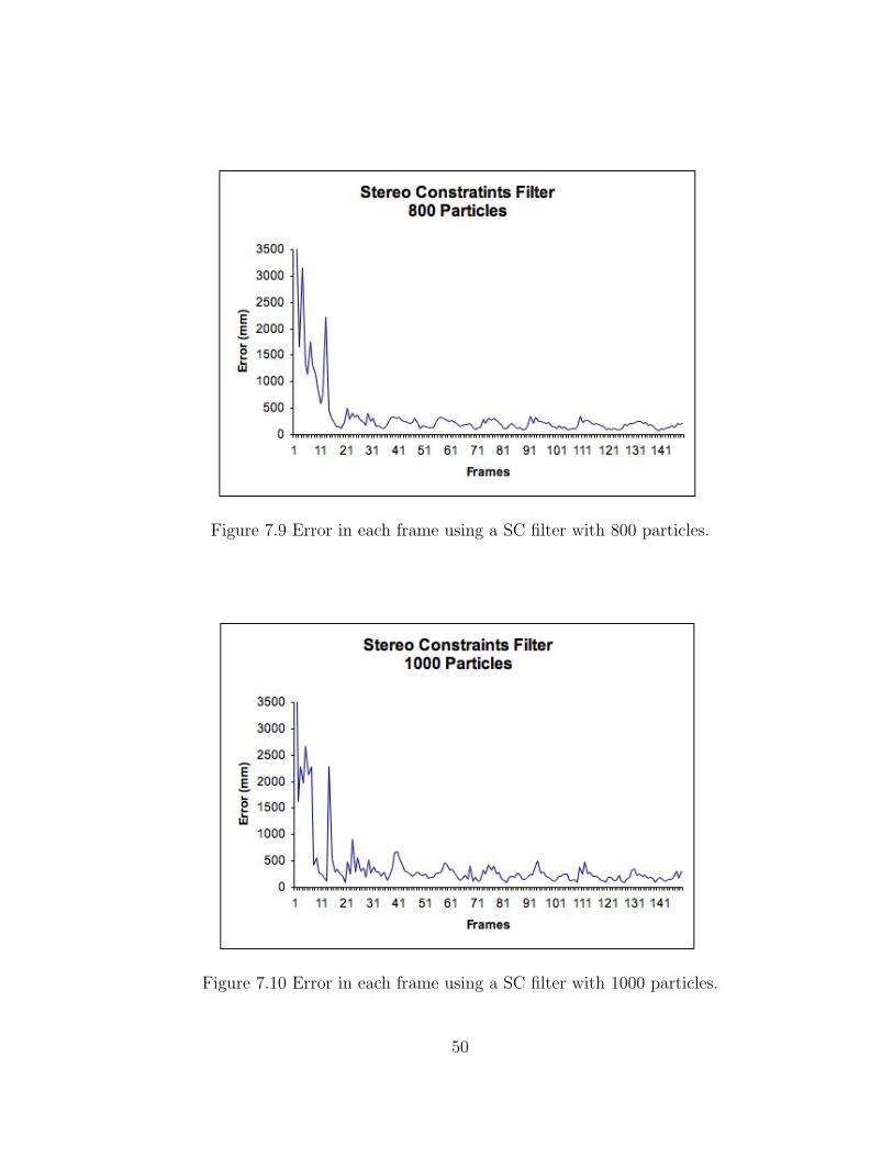
Figure 7.9 Error in each frame using a SC filter with 800 particles.
Figure 7.10 Error in each frame using a SC filter with 1000 particles.
50

Figure 7.11 Error in each frame using 3D filter with 200 particles.
Figure 7.12 Error in each frame using 3D filter with 400 particles.
51
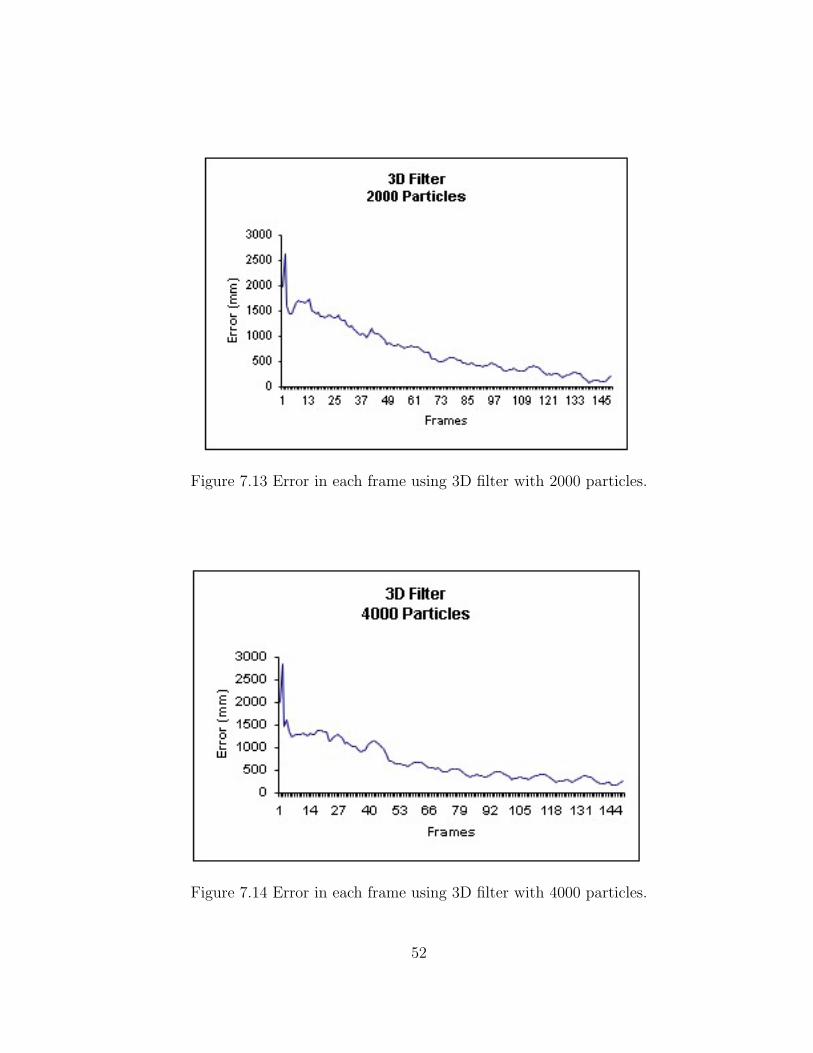
Figure 7.13 Error in each frame using 3D filter with 2000 particles.
Figure 7.14 Error in each frame using 3D filter with 4000 particles.
52

Figure 7.15 Errors in each direction in each frame using SC filter.
1000 particles, here the errors are asymptotic errors i.e., the errors once the filter has
homed-in on the object. In this figure it can be observed that the errors in the z direction
are substantially less than for the stereo constraints filter.
7.2 Cluttered Background
In these experiments also a simple pendulum is used, but with a cluttered back-
ground. This setup is shown in Figure 7.17. Figure 7.18, Figure 7.19, Figure 7.20 and
Figure 7.21 show the error in each frame as the tracking continues, with different particle
sets using a stereo constraints filter. Here as the number of particles increases the preci-
sion increases. Figure 7.22, Figure 7.23, Figure 7.24, Figure 7.25, Figure 7.26 Figure 7.27
and Figure 7.28 shows the error in each frame with different particle numbers using a 3D
filter. Here also the precision increases with the increase in the number of particles.
53

Figure 7.16 Error in direction in each frame using 3D filter.
Figure 7.17 Pendulum with cluttered background.
54

Figure 7.18 Average Error in each frame using a SC filter with 200 particles.
Figure 7.19 Average Error in each frame using a SC filter with 400 particles.
55

Figure 7.20 Average Error in each frame using a SC filter with 800 particles.
Figure 7.21 Average Error in each frame using a SC filter with 1000 particles.
56
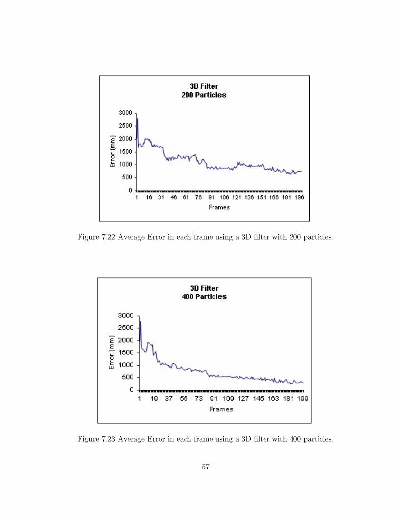
Figure 7.22 Average Error in each frame using a 3D filter with 200 particles.
Figure 7.23 Average Error in each frame using a 3D filter with 400 particles.
57

Figure 7.24 Average Error in each frame using a 3D filter with 800 particles.
Figure 7.25 Average Error in each frame using a 3D filter with 1000 particles.
58

Figure 7.26 Average Error in each frame using a 3D filter with 1500 particles.
Figure 7.27 Average Error in each frame using a 3D filter with 2000 particles.
59

Figure 7.28 Average Error in each frame using a 3D filter with 4000 particles.
7.3 Multiple Objects
In these experiments multiple objects are used. The objects are introduced and
moved away from the cameras’ field of view as the tracking process continues. These
experiments are conducted to demonstrate the stereo constraint filter’s ability to home
in and track new objects as they are introduced into the scene and to re-initialize when
objects get occluded or taken away from the scene. Table 7.2 shows the screen shots of
the tracking process. The pictures in the same row are frames taken at the same instant
of time. Pictures in the left column correspond to the left camera and the right column to
the right camera. The particle locations are represented by the blue dots. In Table 7.2,
the stereo pair in the first row shows the third iteration of the filter and the particles are
spread all over the image. The second row is the tenth iteration and it can be seen that
the particles are homing in on the object. Some particles in the right image are homed
in on the second object also. All the particles drift onto the first object, as shown in the
third row of the table. The subsequent frames show the tracking process as objects are
moved in and out of the scene.
60

Table 7.2 Multiple-Object experiments
61
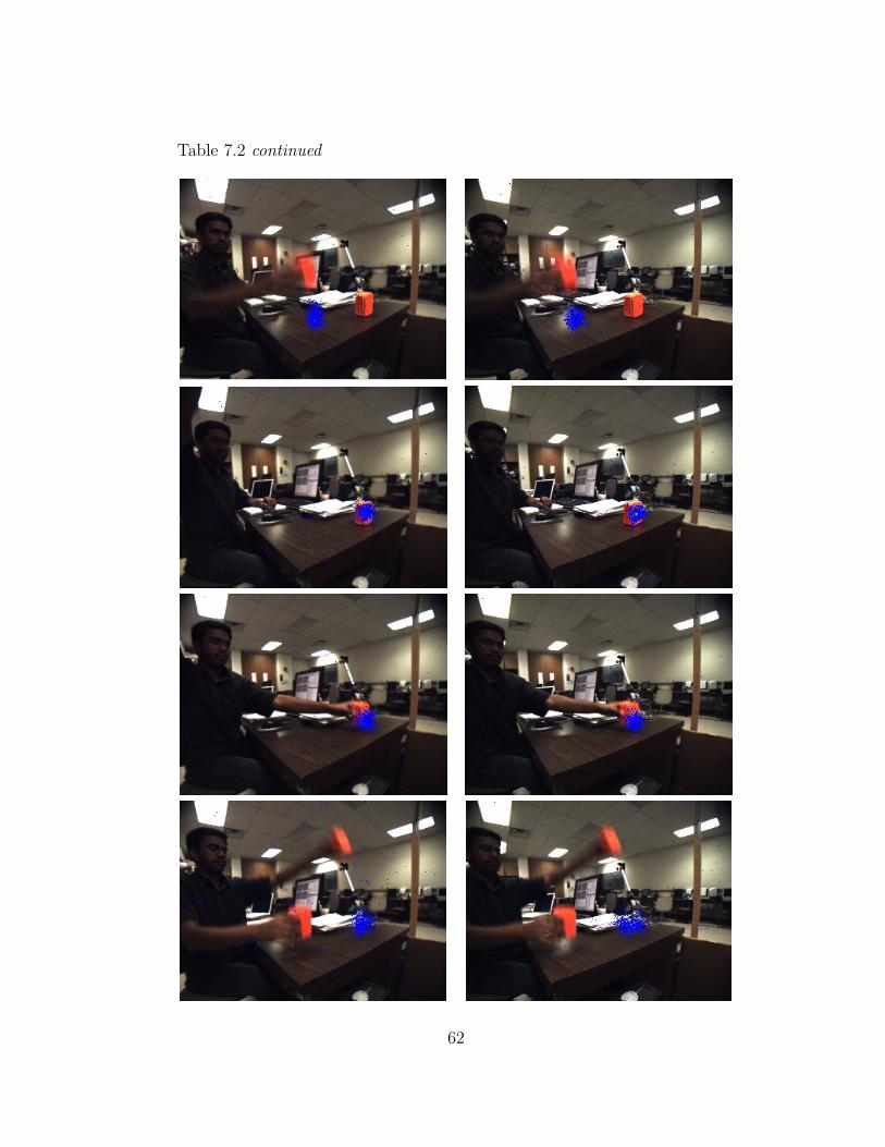
Table 7.2 continued
62

Table 7.2 continued
63

CHAPTER 8
CONCLUSION AND FUTURE WORK
8.1 Conclusions
Vision-based tracking systems have wide ranging applications in robotics, visual
surveillance and manufacturing. With the rapid increase in the computational power
and availability of cheap hardware, more and more computer vision systems are being
developed to automate visual tasks which have previously been performed by human
beings, and to potentially improve their performance. Vision systems are becoming more
robust, but there is long way to go to match the performance levels of human vision.
This thesis is a small advancement towards that goal.
This thesis dealt with tracking objects in a stereo camera system using particle
filters based on the visual cues of the object. The stereo correspondence problem to
track objects in 3D is alleviated in the proposed method by incorporating the stereo
constraints into the particle filter. Two types of filters were used, the stereo constraints
filter and the 3D filter. The results indicate that, the stereo constraints filter homes in
on the objects very fast, but tracking errors are slightly higher when compared to the 3D
filter. The tracking precision in 3D filter is higher, but this filter takes a little longer to
home in on the object.
64

8.2 Future Work
It was seen in the experimental results, that the stereo constraints filter converges
faster on to the object and the 3D filter converges slowly, but its tracking errors are low.
So to take advantage of these properties of the two filters, the stereo constraints filter
could be used to coarse-localize and then to seed a 3D filter to track effectively.
As better observation models are developed they can be incorporated into the
proposed filter to track more robustly and to increase the range of tasks that can be
addressed by this tracking framework.
65
REFERENCES
[1] R. Kasturi and R. C. Jain, Computer Vision : Principles. IEEE Computer Society
Press, 1991.
[2] D. Margaritis and S. Thrun, “Learning to locate an object in 3d space from a
sequence of camera images,” Proc. of Int. Conf. on Machine Learning, pp. 332–340,
1998.
[3] P.Barrera, J.M.Canas, V.Matellan, and F.Martın, “Multicamera 3d tracking using
particle filter,” Int. Conf. on Multimedia, Image processing and Computer Vision,
30march-1april 2005.
[4] P.Barrera, J.M.Canas, and V.Matellan, “Visual object tracking in 3d with color
based particle filter,” Int. Conf. on Pattern Recognition and Computer Vision, 25-
27 february 2005.
[5] P. Perez, J. Vermaak, and A. Blake, “Data fusion for visual tracking with particles,”
Proceedings of IEEE, vol. 92, no. 3, pp. 495–513, March 2004.
[6] S. Spors and R. Rabenstein, “A real-time face tracker for color video.” Utah, USA:
IEEE, May 2001.
[7] J. W. Lee, M. S. Kim, and I. S. Kweon, “A kalman filter based visual tracking
algorithm for an object moving in 3d,” Intl. Conference on Intelligent Robots and
Systems, pp. 342–347, 5-9 Aug 1995.
[8] I. Mikic, M. Trivedi, E. Hunter, and P. Cosman, “Human body model acquisition
and tracking using voxel data,” IJCV, vol. 53, no. 3, pp. 199–233, 2003.
66
[9] E. A. Wan and R. van der Merve, “The unscented kalman filter for nonlinear esti-
mation,” IEEE Symposium on Adaptive Systems for Signal Processing, Communi-
cations and Control, pp. 153–158, October 2000.
[10] B. Stenger, P. R. S. Mendonca, and R. Cipolla, “Model-based 3d tracking of an
articulated hand,” Conf. Computer Vision and Pattern Recognition, vol. 2, pp. 310–
315, December 2001.
[11] J. J. LaViola, “A comparision of unscented and extended kalman filtering for esti-
mating quaternion motion,” Proc. of American Control Conference, pp. 2435–2440,
June 2003.
[12] M. Isard and A. Blake, “Conditional density propagation for visual tracking,” In-
ternational Journal of Computer Vision, vol. 29(1), pp. 5–28, 1998.
[13] Y. Rui and Y. Chen, “Better proposal distributions: Object tracking using unscented
particle filter,” IEEE CVPR, vol. II, pp. 786–793, 2001.
[14] M. Spengler and B. Schiele, “Towards robust multi-cue integration for visual track-
ing,” Machine Vision and Applications, vol. 14, pp. 50–58, 2003.
[15] J. MacCormick, “Probabilistic modelling and stochastic algorithms for visual local-
isation and tracking,” Ph.D. dissertation, University of Oxford, January 2000.
[16] H. Sidenbladh and M. Black, “Learning image statistics for bayesian tracking,” Int.
J. Computer Vision, vol. 54, pp. 183–209, 2003.
[17] J. Sullivan, A. Blake, M. Isard, and J. MacCormick, “Bayesian object localisation in
images,” International Journal of Computer Vision, vol. 44(2), pp. 111–135, 2001.
[18] K. Nummiaro, E. Koller-Meier, and L. V. Gool, “An adaptive color-based particle
filter,” Journal of Image and Vision Computing, vol. 21(1), pp. 99–110, 2003.
[19] K. Nummiaro, E. Koller-Meier, T. Svoboda, D. Roth, and L. V. Gool,
“Color-based object tracking in multi-camera environments.” [Online]. Available:
http://citeseer.ist.psu.edu/648085.html
67

[20] P. Perez, C. Hue, J. Vermaak, and M. Gangnet, “Color-based probabilistic tracking,”
European Conference on Computer Vision (ECCV), pp. 661–675, 2002.
[21] D. Comaniciu, V. Rames, and P. Meer, “Real-time tracking of non-rigid objects
using mean shift,” IEEE CVPR, pp. 142–149, 2000.
[22] F. Dellaert, W. Burgard, D. Fox, and S. Thrun, “Using the condensation algorithm
for robust, vision-based mobile robot localization,” Proc. Conf. Comp. Vision Pat-
tern Rec., pp. 588–594, 1999.
[23] E. Koller-Meier and F. Ade, “Tracking multiple objects using the condensation algo-
rithm,” Journal of Robotics and Autonomous Systems, vol. 34, no. 2-3, pp. 93–105,
2001.
[24] M. Isard and J. MacCormick, “Bramble: a bayesian multiple-blob tracker,” Intl.
Conf. Computer Vision, pp. 34–41, 2001.
[25] A. Gelb, Applied Optimal Estimation. Cambridge Mass: MIT press, 1974, no. ISBN
0 262 70008-5.
[26] M. S. Arulapalam, S. Makell, N. Gordon, and T. Clapp, “A tutorial on particle
filters for online non-linear/non-gaussian bayesian tracking,” IEEE Transactions on
Signal Processing, vol. 50, pp. 174–188, 2002.
[27] L. G. Shapiro and G. C. Stockman, Computer Vision. New Jersey: Prentice Hall,
2001.
[28] D. A. Forsyth and J. Ponce, Computer Vision : A Modern Approach, 1st ed. Pren-
tice Hall, 2001.
[29] O. Faugeras, Three-Dimensional Computer Vision. The MIT Press, 1993, no. ISBN
0-262-06158-9.
[30] J. Canny, “A computational approach to edge detection,” IEEE Transactions on
Pattern Analysis and Machine Intelligence, vol. 8, Issue 6, pp. 679 – 698, 1986.
68

[31] F. Aherne, N. Thacker, and P. Rockett, “The bhattacharyya metric as an absolute
similarity measure for frequency coded data,” Kybernetika, vol. 32, no. 4, pp. 1–7,
1997.
69

BIOGRAPHICAL STATEMENT
Anup S Sabbi received his Bachelor of Engineering degree in Computer Science
and Engineering from RVR and JC College of Engineering, Nagarjuna University, India
in May 2002. He started his graduate studies in August 2002 and received his Master
of Science degree in Computer Science and Engineering from The University of Texas
at Arlington in May 2005. His current research interests include robotic perception,
computer vision and machine learning.
70


