NASA/CR--1998-207933

OARE STS-94 (MSL-1R) Final Report

James E. Rice

Canopus Systems, Inc., Ann Arbor, Michigan

Prepared under Contract NAS3-26556

National Aeronautics and

Space Administration

Lewis Research Center

June 1998

https://ntrs.nasa.gov/search.jsp?R=19980203951 2018-06-26T17:32:44+00:00Z

NASA Center for Aerospace Information7121 Standard Drive

Hanover, MD 21076Price Code: A03

Availablefrom

National Technical Information Service

5287 Port Royal Road

Springfield, VA 22100Price Code: A03

TABLE OF CONTENTS

1.0 INTRODUCTION .......................................................................................................................................... I

1.10ARE SYSTEM FEATURES .............................................................................................................................. 1

1.2 COORDINATE SYSTEMS ................................................................................................................................... 1

1.3 SENSOR MEASUREMENT PARAMETERS ......................................................................................................... 2

2.0 STS-94 0MSL-IR) MISSION RESULTS ..................................................................................................... 2

2.1 STS-94(MSL-IR) MISSION PLAN .................................................................................................................. 2

2.2 STS-94 ACTUAL MISSION DESCRIPTION ....................................................................................................... 3

2.3 STS-94 DATA ANALYSIS ................................................................................................................................. 3

2.4 ORBITER BODY AXIS ACCELERATIONS RESULTS .......................................................................................... 5

2.5 STS-94 ANOMALOUS PERFORMANCE ............................................................................................................ 5

3.00ARE ACCURACY ANALYSIS ................................................................................................................ 10

3.1 BIAS ERRORS .................................................................................................................................................. 10

3.2 SCALE FACTOR ERRORS ................................................................................................................................ l0

3.3 QUASI-STEADY ACCELERATION MEASUREMENTS ...................................................................................... 10

4.0 REFERENCES ............................................................................................................................... 11

TABLE OF FIGURES

Figure 1. STS-94 Instrument (Sensor Head) Temperature ................................................................................... 4

Figure 2a. Quasi-Steady Acceleration at the OARE Location, MET 0-96 Hours .................................................. 6

Figure 2b. Quasi-Steady Acceleration at the OARE Location, MET 96-192 Hours .............................................. 7

Figure 2c. Quasi-Steady Acceleration at the OARE Location, MET 192-288 Hours ............................................ 8

Figure 2d. Quasi-Steady Acceleration at the OARE Location, MET 288-384 Hours ............................................ 9

TABLE OF TABLES

Table 1. OARE Sensor Ranges and Resolutions .................................................................................................... 2

APPENDIX A

OARE DATA CALIBRATION .................................................................................................................. A I-A I 1

1.0INTRODUCTION

The report is organized into sections representing the phases of work performed in analyzing theSTS-94 (MSL-IR) results. STS-94 (MSL-IR) is a reflight of the STS-83 (MSL-I) mission which

was terminated early because of a fuel cell problem. Section I briefy outlines the OARE system

features, coordinates, and measurement parameters. Section 2 describes the results from STS-94.

The mission description, data calibration, and representative data obtained on STS-94 are presented.

Also, the anomalous performance of OARE on STS-94 is discussed. Finally, Section 3 presents a

discussion of accuracy achieved and achievable with OARE. Appendix A discusses the calibration

and data processing methodology in detail.

1.10AR£ System Features

The Orbital Acceleration Research Experiment (OARE) contains a tri-axial accelerometer which

uses a single free-floating (non-pendulous) electrostatically suspended cylindrical proofmass. The

accelerometer sensor assembly is mounted on dual-gimbal platform which is controlled by a

microprocessor in order to perform in-flight calibrations. Acceleration measurements are processed

and stored in the OARE flight computer memory and, simultaneously, the unprocessed data are

recorded on the shuttle payload tape recorder. These raw data are telemetered periodically to ground

stations at several hour intervals during flight via tape recorder playback (data dumps).

OARE's objectives are to measure quasi-steady accelerations, to make high resolution low-frequency

acceleration measurements in support of the micro-gravity community, and to measure Orbiter

aerodynamic performance on orbit and during reentry. There are several features which make theOAP,.E well suited for making highly accurate, low-frequency acceleration measurements. OARE is

the first high resolution, high accuracy accelerometer flight design which has the capability to

perform both bias and scale factor calibrations in orbit. Another design feature is the OARE sensor

electrostatic suspension which has much less bias temperature sensitivity than pendulousaccelerometers. Given the nature of the OARE sensor and its in-flight calibration capability, OARE

stands alone in its ability to characterize the low-frequency environment of the Orbiter with better

than 10 nano-g resolution and approximately 50 nano-g on-orbit accuracy.

1.2 Coordinate Systems

Two coordinate systems are used in this report -- the OARE axes centered at the OARE sensor

proofmass centroid and the Orbiter aircrat_ body axes centered at the Orbiter's center of gravity. The

direction from tail to nose of the orbiter is +X in both systems. The direction from port wing to

starboard wing is +Z in the OARE system and +Y in the Orbiter body system. The direction from

the Orbiter belly to the top of the Orbiter fuselage is +Y in the OARE system and -Z in the Orbiter

body system. This sensor-to-body coordinate alignment referred to above is the nominal flight

alignment and was utilized for OARE data collection during STS-94.

In discussions of OARE calibrations of bias and scale factor, the OARE reference system is used.

However, the fight acceleration data are given in the Orbiter body reference system. The signconvention is such that when there is a forward acceleration of the Orbiter (such as the OMS firing),

this is then reported as a positive X-axis acceleration, even though a free particle may appear to

move in the -X direction relative to the accelerating shuttle. All accelerations given in this report

refer to the OARE location.

1.3 Sensor Measurement Parameters

There are three sensor ranges, A, B, and C, for each OARE axis, which are controlled by auto-

ranging software logic. The full scale ranges and resolutions (corresponding to one count) are givenin Table 1. In order to denote in the data when the sensor channel is driven into saturation, the

output is set to 1.5 times full scale of range A with the sign of the saturation signal included.

Table 1. OARE Sensor Ranges and Resolutions

Nominal Full Scale Rangein micro-Gs

Range X-Axis Y & Z Axes

A 10,000 25,000

B 1,000 1,970

C 100 150

Resolution in nano-Gs

SFN in nano-Gs/count

Range X-Axis Y & Z AxesA 305.2 762.9

B 30.52 60.12

C 3.052 4.578

2.0 STS-94 (MSL-1R) MISSION RESULTS

This section describes the results from STS-94 as derived from post-flight processing of the trim-

mean OARE acceleration data stored on the on-board EEPROM. During the mission, preliminary

calibrations and accelerations were reported in near-real time by NASA Lewis Research Center using

the telemetered data from the payload tape recorder.

2.1 STS-94 (MSL-1R) Mission Plan

The STS-94 adaptation parameters anticipated a mission of up to 17 days long. In order to make

better use of the calibration time, the soRware was modified prior to STS-73 so that only C-range

calibrations would occur in the "Quiet" mode, and calibrations would occur on all three ranges

during the "Normal" mode. Since past experience had indicated that the Scale Factor had minimal

variations and that, on-orbit, the instrument remains almost entirely in the C-range, the adaptation

parameters were selected to use most of the allotted calibration time for C-range bias calibrations in

order to obtain the most accurate measurements possible. When operating in the "Quiet" mode, C-

range bias calibrations are to be performed every 158 minutes, and a bias calibration begins within

one minute after the "Quiet" mode is asserted. A C-range scale factor calibration is to be performed

after every 15th bias calibration in the "Quiet" mode. In the "Normal" mode, a full bias calibration is

to be performed ever)' 432 minutes, and a full scale factor calibration is performed after every 6thbias calibration.

REPORT DOCUMENTATION PAGE FormApprovedOMB No. 0704-0188

Pubac re_ burr_ f_r _is c_e_i_n of k_rrna_ _ e_tirn_ted to _vemge1_r _ _ _ _ _ _ _ _s_ _ _ _ _gatheringand maintoir_g the data needed, and completingand reviewingthe ootlec0onof rnfocmation. Send commentsrlKlm_1:gb"dsl_rden utlmem or lu'tyother sspect of this¢ohctimt of kdormltion, includingsuggel_ for re¢.¢i_ _ burden, to Wml_ngton _=lerl Sendce¢ Directoratelot InformalJonOperationsand I:lepocts,1215 JeflecaonDeW Highway, Sule 1204. Arlington.VA 222_-4302, and to _ OfSce o_Managementand Bu<k_. Pmm,_ R_uct_ Protect (0704-01_). Wuh_ton, DC 2O503.

1. AGENCY USE ONLY (Leave b/ank) 2. REPORT DATE

June 19984. TITLE AND SUBTITLE

OARE STS-94 (MSL-1R) Final Report

6. AUTHOR(S)

James E. Rice

7. PERFORMING ORGANIZATION NAME(S) AND ADDRESS(ES)

Canopus Systems, Inc.

Ann Arbor, Michigan

9. SPONSORING/MONITORING AGENCY NAME(S) AND ADDRESS(ES)

National Aeronautics and Space AdministrationLewis Research Center

Cleveland, Ohio 44135-3191

3. REPORT TYPE AND DATES COVERED

Final Contractor Report5. FUNDING NUMBERS

WU-963-60-0C-00

NAS3-26556

18. PERFORMING ORGANIZATION

REPORT NUMBER

E-11205

10. SPONSORING/MONITORINGAGENCY REPORT NUMBER

NASA CR_1998-207933

11. SUPPLEMENTARY NOTES

Project Manager, William O. Wagar, Microgravity Science Division, NASA Lewis Research Center, organization code

6727, (216) 433-3665.

12a. DISTRIBUTION/AVAILABILITY STATEMENT

Unclassified - Unlimited

Subject Category: 19 Distribution: Nonstandard

This publication is available from the NASA Center for AeroSpace Information, (301) 621-0390.

12b. DISTRIBUTION CODE

13. ABSTRACT (Maximum 200 words)

The report is organized into sections representing the phases of work performed in analyzing the STS-94 (MSL-1R)results. STS-94 (MSL-1R) is a reflight of the STS-83 (MSL-1) mission which was terminated early because of a fuel cell

problem. Section 1 briefly outlines the OARE system features, coordinates, and measurement parameters. Section 2describes the results from STS-94. The mission description, data calibration, and representative data obtained on STS-94

are presented. Also, the anomalous performance of OARE on STS-94 is discussed. Finally, Section 3 presents a discussionof accuracy achieved and achievable with OARE. Appendix A discuss the calibration and data processing methodology indetail.

14. SUBJECT TERMS

Acceleration measurement; Microgravity; Space sensors

17. SECURITY CLASSIFICATIONOF REPORT

Unclassified

NSN 7540-01-280-5500

18. SECURITY CLASSIFICATIONOF THIS PAGE

Unclassified

15. NUMBER OF PAGES

2916. PRICE CODE

A0319. SECURITY CLASSIRCATION 20. LIMITATION OF ABSTRACT

OF ABSTRACT

Unclassified

Standard Form 298 (Rev. 2-89)

Prescribed by ANSI Stcl. Z39-18298-102

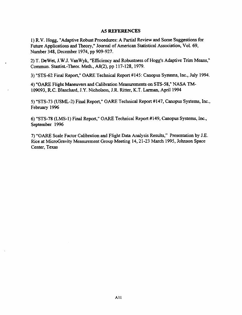
A5 REFERENCES

1) R.V. Hogg, "Adaptive Robust Procedures: A Partial Review and Some Suggestions for

Future Applications and Theory," Journal of American Statistical Association, Vol. 69,

Number 348, December 1974, pp 909-927.

2) T. DeWet, J.W.J. VanWyk, "Efficiency and Robustness of Hogg's Adaptive Trim Means,"

Commun. Stastist.-Theor. Meth., A8(2), pp 117-128, 1979.

3) "STS-62 Final Report," OARE Technical Report #145: Canopus Systems, Inc., July 1994.

4) "OARE Flight Maneuvers and Calibration Measurements on STS-58," NASA TM-

109093, R.C. Blanehard, J.Y. Nicholson, J.R. Ritter, K.T. Larman, April 1994

5) "STS-73 (USML-2) Final Report," OARE Technical Report #147, Canopus Systems, Inc.,

February 1996

6) "STS-78 (LMS-1) Final Report," OARE Technical Report #149, Canopus Systems, Inc.,

September 1996

7) "OARE Scale Factor Calibration and Flight Data Analysis Results," Presentation by J.E.

Rice at MicroGravity Measurement Group Meeting 14, 21-23 March 1995, Johnson Space

Center, Texas

All

2.2 STS-94 Actual Mission Description

Launch for STS-94 was at about 2:02 p.m. EDT on 1 July 1997. The actual length of the STS-94

mission was 376.74 hours or about 15 days and 16 3/4 hours with touch down at 6:46:34 a.m. EDT

on 17 July 1997. Shutdown occurred in REENTER mode under the condition of"re-capture durationerror" in sub-mode 4. This means that the OARE instrument continued to collect data until the Y-

axis signal was saturated for at least 2 minutes in the final REENTER sub-mode. This is considered

normal termination of the mission and represents adequate adaptation parameter settings for the

reenter file size and correct timing of the reenter discrete.

OARE was powered on during the launch. Since the Quiet mode was set at MET 5.96 hours, the

necessary elapsed time of 432 minutes has not occurred from power-on to generate a Normal fullbias calibration or scale factor calibration of all ranges on OARE early in the mission. The Quiet

Mode lasted until about MET of 133.55 hours when the system was again switched to Normal mode.

During STS-94, 82 C-range bias measurements were made. 34 bias measurements were made on

the A and B ranges after 140.8 hours MET. There were 10 and 7 scale factor measurements made on

the C and A&B ranges, respectively.

All engineering parameter values were within normal range. Hardware performance was normal.

2.3 STS-94 Data Analysis

This section treats the several analyses carried out on the STS-94 flight data and summarizes the

significant results. The processed acceleration data have already been delivered to the Microgravity

Measurements and Analysis Branch Program (MMAP) at NASA Lewis Research Center.

The Orbital Acceleration Research Experiment (OARE) is designed to measure quasi-steady

accelerations from below 10 nano-g up to 25 milli-g where quasi-steady indicates the frequency

range from 10-5 to 10-I Hz. To accomplish this, the sensor output acceleration signal is filtered with

a Bessel filter with a cut-off frequency of 1 Hz. and cut-offrate of 120 dB per decade The output

signal is initially processed at 10 samples per second and is then further processed and digitallyfiltered onboard the OARE instrument with an adaptive trimmean filter prior to the normal EEPROM

storage. The trimmean data samples cover 50 second periods every 25 seconds. The regular 10

sample per second data were recorded on the payload tape recorder.

In flight, the OARE instrument is subjected to higher amplitude and higher frequency accelerations

(due to the Reaction Control System (RCS) thrusters, structural vibrations, and crew activities) in

addition to the quasi-steady accelerations due to the gravity gradient, on-orbit drag, slow shuttle

body rotations, and long period venting.

In order to obtain the optimum estimate of the quasi-steady acceleration under these conditions, a

robust adaptive estimator has been implemented as part of the OARE analysis system. The particular

estimator used is known as the Hogg Adaptive Trimmean estimator [1,2]. The bias estimate using

the trimmean estimator of the acceleration is critical to the accuracy of acceleration measurements.

During all previous missions, the data have been processed using the trimmean estimator because it

provides the best estimate of the quasi-steady acceleration.

It has been the conventional wisdom that the quasi-steady acceleration effects are the most relevant

to fluid experiments (as well as others) since in these experiments the processes have a finite reaction

time and are believed to be quite insensitive to high frequency accelerations. However, although the

structural vibrations and crew activities induce only AC components of acceleration, the thruster

firings produce a significant DC component of acceleration even though it is mostly high frequencyrelative to 0.1 Hz. The Trimmean filter tends to exclude these measurements from the 50 second

trimmean averages, and thus, these short thruster firings do not normally appear in the trimmean

processed data appearing in this report. In order to quantify these effects, the 10 sample per second

data recorded on the payload taper recorder would need to be processed. This has not been done in

this report, hut was done on STS-75 where the EEPROM trimmean data were lost [8].

Thus, for STS-94 (MSL-IR) the only measure of acceleration presented is the 50 second trimmean

average calculated every 25 seconds as has been done on all previous OARE missions.

A detailed discussion of the data analysis undertaken for STS-94 is presented in Appendix A along

with the bias estimates using estimated measurement errors based upon the distributions of the

measured data. This mission incorporated a full weighted least squares estimate of bias as was done

on STS-73. [6]

The complete digital acceleration data presented in this report, as well as the raw payload tape

recorder data at 10 samples per second which have not been processed by the trimmean filters, are

available from the Microgravity Measurements and Analysis Program (MMAP) at NASA LewisResearch Center.[7]

The temperature environment was relatively benign except for the large temperature excursion

during the initial thermal pulse generated during launch on STS-94. The instrument temperature in

degrees Celsius (measured on the proofmass housing) is shown in Figure 1.

50F

45 T ........

g 40 ..................... 10

.t:: 35 -. ................... ii

30 ,

10 .... , , ,

OARE Sensor Head Temperature

20 ............................................... __ ..

............ i ........... i , , , i .......... |u ! ! i a u !

0 24 48 72 96 120 144 168 192 216 240 264 288 312 336 360 384

MET in Hours

Figure 1. STS-94 Instrument (Sensor Head) Temperature.

2.4 Orbiter Body Axis Acceleration Results

The accelerations measured by OARE at the OARE location in the Shuttle Body Axes coordinate

system ( X, toward the nose; Y, toward the starboard wing; Z, down through the belly) are shown in

Figures 2a through 2d.

Figures 2a through 2d show the trimmean acceleration measured at the OARE location during the

entire OARE operational time. This measure of acceleration represents the acceleration due to the

quasi-steady forces in that the larger short-period pulses are effectively removed from the data by

this filter. The acceleration measurement set has small gaps in it during the periods when bias and

scale factor calibrations are being made.

This gives an overview of the data, but it may not be in enough detail to meet the requirements of

each experimenter. Also, the experimenter may want the acceleration transformed to the particular

experiment's location. For additional detail, the complete set of data is available from the PIMS

Group at Lewis Research Center. [7] The low frequency accelerations can also be calculated at the

experimenter's location by the PIMS group using the OARE measurements and other shuttle

parameters. Canopus Systems would be happy to answer any questions about OARE operations or

the processed OARE data at the OARE location.

2.5 STS-94 Anomalous Performance

OARE's performance on STS-94 was similar to that on previous missions The Z-axis C-range scale

factor calibration was still affected by jitter to a small degree.

(3

¢;

¢,-0

(9

03totO<

-2

-4

0 12 24 36 48 60 72 84 96

MET in Hours

u)

(.9

t-

t-O

03

03toto

<

8

6

4

2

0

-2

-4

0

• ' "_' ' ' t " ' " _ " " I' I i" "ill ' :r

, Orbter Y-A is .i........ _ -- i!- _ *

I ' i ii : _

i..! ......... _ !......lii_ ,

: = , I:_ ' _ I BI/ /!' , =

" F,t I 'll12 24 36 48 60 72 84 96

MET in Hours

6

(/)(3 4

t- 2

t-o 0

03 -2

03to -4to<

-6

Orbiter ._-Axis i ti iI

r

I1_1IIIIll_.I]

IHiIIII1_1till

0 12 24 36 48 60 72 84 96

MET in Hours

Figure 2a. Quasi-Steady Acceleration at the OARE Location, MET 0-96 Hours.

r/}

(.9

¢-

Oo_

t..

Q)

O

<

8

6

4

2

0

-2

-4

II i

._h=.=..a..=._...--

96

ill .....,,11 ,

108 120 132 144

'I i

-=_!I il

156

1 ii

I!

I .I

168 18t 192

MET in Hours

(/)

O

t-.D

¢-O

°m

t.,.

t_

<

8

6

4

2

0

-2

-4

96

," _ .... ! "i" ! , ' T 'Axis: _ _ Or Y- _ , ......... _ ......

i ' I= t ! ...... ! ,

: 17 i i

' ': ' ' * ' ' I , , , i , , i , ,108 120 132 144 156 168 180 92

MET in Hours

C/)

(.9

t'-

t-O

t.-

OO

<

-2

-4

-6

6 , , , , , , ,

4 ................ Orbiter Z-Axis

2

0

96

=±,.Jh..._..,,, .... ,._-_,L......

I i

101 120

I i i, I

132 144

I I I

156 168 180 192

MET in Hours

Figure 2b. Quasi-Steady Acceleration at the OARE Location, MET 96-192 Hours.

1/)

(.9

r"°m

t-o

om

Q)

(UrO¢.)

<

8

6

4

2

0

-2

-4

192

P.i,I

!

OJ'hit#r

HII '11[I , ',Ill

T[Ilili_11ltll,+,lilllli,

I I | * =

204 216 228 240

[

.............................; ! ........

i I ,

252 264 276 288

MET in Hours

¢/)

(3

c

t-O

tO

oo<

8

6

4

2

0

-2

-4

192

I- _ : I ' ! II: ; i i i Orbitert Y-;_xlis i *,

/ ! i F Jl ; :i : i

I ] i : IJ : ;!i! i -- _ :! ! : iI i: _ i

' I " . .:, [ . +_ .1 1 . .I. , .204 21_ 228 240 252

MET in Hours

.]i

....F_F264

iF!i+:i+i+276 288

(3

¢-.D

t-O

PO)

(Uof.)

<

4

2

0

-2

-4

-6

192

'_'*_'Jlti,,L,.

204

I ! !

'Orbiter Z-Axis............................................... r+

216

........... +..................................

"!'+I'i,228 252240

II![ill °264

MET in Hours

I

276 288

Figure 2c. Quasi-Steady Acceleration at the OARE Location, MET 192-288 Hours.

8

4._¢

2_ o

-4

288

.... ,_ lr _ll [I ILILiII

I t 'i I i i

300 312 324 336 348 360 372 384

MET in Hours

(/)

(,9:::3

E:

f-O

I,,--

toto<

8

6 ...........

4 ....

2

-2

-4 ,

288

t! : Orb,terY-Ax_,s _i I, ,W _:1

..... : " i ! ;

J ,J .,';I ___ ' ; ' i I! ; I_ ........

I " ' ' I ' * ' I I

300 312 324 336 348 360 372 _84

MET in Hours

O

¢-

¢-O

.m

i,-

®

toto

<

6 ,

4-

2

0

-2

-4

-6288

I iOrbiter Z-Axis._ ............. _ ............. i ................................

• i _ .........

I '

, ...... _ " " " i '300 312 324 336

i .i , I

348 360 372

MET in Hours

384

Figure 2d. Quasi-Steady Acceleration at the OARE Location, MET 288-384 Hours.

9

3.00ARE ACCURACY ANALYSIS

The OARE instrument provides high resolution measurements of sensor input axes accelerations,

3.05 nano-Gs in the X-axis and 4.6 nano-Gs for the Y and Z axes. The accuracy of these

measurements is primarily determined by the degree to which the instrument can be calibrated

over the time period of the measurements. Major sources of potential errors are the accuracyobtainable from the bias and scale factor calibrations.

3.1 Bias Errors

On STS-94, the bias was measured 82 times. From these measurements, the true bias was

estimated by the fitting procedure discussed in Appendix A. Potential errors in these bias

estimates arise from the statistical nature of the bias measurements as well as from potential

systematic errors which have not been identified. Based upon the analysis contained in Appendix

A, we estimate that the bias errors on range C are approximately 50 nano-Gs. These are

consistent with the earlier analysis contained in the STS-65 Final Report [5].

3.2 Scale Factor Errors

In the microgravity environment of the Orbiter, the quasi-steady trimmean acceleration

measurements are typically on the order of 1 micro-g or less. Under these conditions, the bias

errors are larger than the scale factor errors.

Measurements of the scale factors made during flight and those on the ground are now consistent

to within 1 to 2 percent. We estimate the scale factor errors to be about 1 to 2 percent of the

measured acceleration. These could be reduced with further study. At a 1 micro-g level, this

corresponds to a 10 to 20 nano-G error. These should be added in quadrature with the bias errors.

So overall, this gives estimated errors for the on-orbit acceleration measurements of about 50 to 60nano-Gs. Scale Factors were estimated from the Scale Factor measurements made on this mission.

3.3 Quasi-Steady Acceleration Measurements

As indicated, the primary OARE data recorded on the flight computer is processed through an

adaptive trimmean filter. This trimmean filter provides a near optimum estimate of the mean of

the quasi-steady acceleration population of measurements over the 50 second sampling period.

This estimate is particularly beneficial in the calculation of the bias estimate and the estimate of

the quasi-steady acceleration due to orbital drag, gravity gradient, and slow body rotations.

However, it tends to reject the effects of crew activity, thruster firings, and other exogenous

events. Experimenters may be interested in the regular average of the acceleration measurements

over the 50 second sample period or other acceleration measurement metrics. In any case, the

regular average and other filters could be applied to the payload tape recorder data for those

periods where the data exist.

10

4.0 REFERENCES

l) R.V. Hogg, nAdaptive Robust Procedures: A Partial Review and Some Suggestions for Future

Applications and Theory," Journal of American Statistical Association, Vol. 69, Number 348,

December 1974, pp 909-927.

2) T. DeWet, J.W.J. VanWyk, _Efficiency and Robustness of Hogg's Adaptive Trim Means,"

Commun. Stastist.-Theor. Meth., A8(2), pp 117-128, 1979.

3) _STS 62 Final Report," OARE Technical Report #145: Canopus Systems, Inc., July 1994.

4) "OARE Flight Maneuvers and Calibration Measurements on STS-58," NASA TM-109093,R.C. Blanchard, J.Y. Nicholson, J.R. Ritter, K.T. Larman, April 1994.

5)_STS-65 Final Report," OARE Technical Report #146, Canopus Systems, Inc., November1994.

6) "STS-73 (USML-2) Final Report," OARE Technical Report #147, Canopus Systems, Inc.,

February 1996.

7) Microgravity Measurement and Analysis Program (MMAP) at Lewis Research Center. Program

Manager of Principle Investigator of Microgravity Services (PIMS) is Duc Truong, (216) 433-

8394. E-mail to duc.truong@lerc.nasa.gov. Data file server is beech.lerc.nasa.gov.

8) _STS-75 (USMP-3) Final Report," OARE Technical Report #148, Canopus Systems, Inc., June1996.

9) "STS-78 (LMS-1) Final Report," OARE Technical Report #149, Canopus Systems, Inc.,

September 1996.

1(3) "STS-83 (MSL-1) Final Report," OARE Technical Report #150, Canopus Systems, Inc., May1997.

11

APPENDIX A

OARE DATA CALIBRATION AND PROCESSING

This Appendix reviews the methods used to calculate the Orbiter body triaxial acceleration

based on the OARE instrument measurements which were recorded on the EEPROM,

downloaded, and then processed by Canopus Systems. The method of estimating the sensor

bias has evolved over the past several missions; STS-73 was the first mission where a full

weighted least squares methodology has been implemented in estimating the instrument bias.

The Appendix begins with the instrument model (A1), discusses the trimmean filter used in

processing the raw OARE accelerometry data (A2), presents the weighted least squares

estimate of the bias of the instrument (A3)and finally presents a short discussion of Scale

Factor calibration (A4).

AI INSTRUMENT MODEL

The OARE instrument acceleration for each axis and range is calculated from an equation of

the form

A A = -SF C * SF N * (CTS - 32768 - BIAS) (eq. 1), where

A A is the calibrated actual acceleration in uGs,

SF C is the Scale Factor Calibration term,

SF N is the Nominal Scale Factor in uGs per count,CTS is the counts out of the instrument A/D converter, and

BIAS is the estimated Bias in counts as a function of time and temperature,

where each of the terms is dependent upon the particular axis and range.

In the above equation, the number 32768 appears because the 16-bit A/D converter is single-

ended; this value is the offset required to obtain a zero measured acceleration for a zero input

acceleration when there is no bias.

An Actual Scale Factor SF A term is defined by

SF A = SF C * SF N (eq. 2).

Values of the nominal scale factor, SFN, are given in Table 1 of the main report for each

OARE axis and range. Values of SF C for the OARE X, Y, and Z axes are approximately

1.02, 1.11, and 1.10, respectively, but are determined through calibration on each STS

mission for each axis and range.

The output of the A/D converter provides a raw digital acceleration data sample which is

effectively processed at a rate of 10 times per second. Data are normally stored on the

EEPROM at a rate of once every 25 seconds, and these data represent the trimmean filtered

estimate of the quasi-steady acceleration value over a 50-second period.

AI

A2 HOGG ADAPTIVE TRIMMEAN FILTER USED IN PROCESSING OARE

ACCELERATION MEASUREMENTS

The OARE instrument is designed to measure the quasi-steady acceleration from below 10

nano-Gs up to 25 milli-Gs and over the quasi-steady bandwidth from 10 "s to l0 q Hz. The

quasi-steady acceleration components of primary interest are those due to gravity gradient,

on-orbit drag, inertial rotations, and perhaps long period venting or gas leaks. However, the

instrument is subjected to higher amplitude and higher frequency accelerations (such as

structural vibration, station keeping thruster firings, and crew effects) in addition to the quasi-

steady accelerations. These higher level accelerations are not well characterized nor

statistically invariant over the OARE measurement periods.

In order to obtain a more optimum estimate of the quasi-steady acceleration under the

conditions of intermittent thruster firings and crew activities, a robust adaptive estimator has

been implemented. For a discussion of robust estimators, see Reference 1. The particular

estimator implemented in OARE is known as the Hogg Adaptive Trimmean estimator and isdescribed in more detail in Reference 2.

In essence, the trimmean adaptive filter removes a percentage of the distribution from each

tail and then calculates the mean of the remaining distribution. It first measures the departure

of the sample distribution from a normal (Gaussian) distribution as measured by a parameter

called Q, then adaptively chooses the amount of the trim to be used on the distribution, and

finally calculates the mean of the remaining distribution after the trim. This filter is designed

to remove the effect of a contaminating distribution (such as a thruster firing) superimposed

on a normal distribution (of instnunent noise, high frequency vibrations, crew activities,

quasi-steady accelerations, etc.),

As implemented, Q is defined by the following equation:

Q = [u(20%) - L(20%)]/[U(50%) - L(50%)] (eq. 3), where

U(X%) is the average of the upper X% of the ordered sample, and

L(X%) is the average of the lower X% of the ordered sample.

In the OARE case, the ordered sample has been a sample of 500 acceleration measurements

of the A/D output over a 50-second measurement period.

Q is a measure of the outlier content in the sample. For a Gaussian distribution, Q is 1.75;

for samples which have larger tails, Q > 1.75. The value of Q is used to estimate the extent

that the quasi-steady acceleration measurements may be contaminated by thruster firings,

crew activities, etc.

In order to improve the estimate of the quasi-steady acceleration, a trimmean is used to

estimate the mean of the quasi-steady population. A trim parameter alpha is determined by

the following algorithm:

A2

0.05 for Q <= 1.75

alpha(Q) = 0.5 + 0.35* (Q-1.75)/(2-1.75) for 1.75 < Q < 2.0 (eq. 4)

0.4 for Q >= 2.0,

where alpha is the fraction of the distribution which is trimmed off each tail of the ordereddistribution before the mean of the remainder of the distribution is calculated.

Then, for an underlying distribution of n points or measurements with a value of alpha, the

trimmean is given by

trimmean = [X(k+l) + X (k+2) + ..... + X(n.k)]/(n-2*k ), (eq. 5),

where k = alpha * n (eq. 6) and

X(i), X(i+l),..., X(n ), is the ordered set ofn points making up the sampledistribution.

In summary, OARE measures the quasi-steady level of acceleration for each axis every 25

seconds by taking the trimmean of 50 seconds of A/D counts (500 samples in total) according

to equations 3 through 6, and then substituting this trimmean for CTS in equation 1. It

should be noted that for large pulses in one direction, the effect of the trimmean is to shift the

estimate of the mean; it does not preserve the DC component in this case.

The trimmean is particularly appropriate for estimating the bias of the OARE instrument,since one wishes to remove the effect of the thruster on the bias measurement if a thruster

firing should occur during the bias measurement period.

Data recorded on the EEPROM and available to support the acceleration calculations include

the trimmean of the 50-second distribution every 25 seconds, the Q of this sample

distribution, the Average Deviation from the trimmean of the distribution used to calculate

the trimmean, the instrument temperature, the Mission Elapsed Time (MET), and numerous

housekeeping parameters.

The widths of the 500 sample distributions (as measured by the standard deviations) are

almost entirely due to the environment aboard the shuttle and not due to sensor noise. This

has been illustrated in the figures of the STS-78 Final Report [6]. On STS-78, the whole

crew had common sleep periods; this gave rise to very small variations in the data obtained

during a sleep period. During these periods, the instrument output is extremely quiet as

opposed to periods when there is crew activity. On most missions as on STS-94, the crew

has been active 24 hours per day and consequently noisier data from a quasi-steady point-of-

view has resulted.

A3 BIAS MEASUREMENTS AND ESTIMATED MEASUREMENT ERRORS

As can be seen in Equation 1, the calculated acceleration depends upon the instrument bias.

This is a critical parameter in accelerometers that are designed to measure quasi-steady or DC

A3

accelerations below 1 milli-G. For on-orbit conditions, the typical quasi-steady or DC

acceleration is less than 1 micro-G. Thus, the bias estimate is absolutely critical to accurate

acceleration measurements in this regime.

The OARE accelerometer uses an electrostatic.ally suspended proofmass in order to minimize

the effects of temperature and mechanical suspension hysteresis on the bias. In addition,

OARE incorporates a two-axis gimbal calibration table by which the OARE instrument can

be calibrated on-orbit for bias and scale factor in each of its three axes.

A3.1 Bias Measurements

The bias measurement for a single axis consists of the following sequence: 1) measuring the

acceleration output in trimmean counts for 50 seconds in the normal table position for a given

axis (called BIASN), 2) rotating the input axis 180 °, and then 3) measuring the acceleration

output in trimmean counts (called BIAS I , for inverted position). Assuming that the actual

input acceleration remains constant during this period (about 125 seconds), as might be

expected for quasi-steady accelerations, then the bias can be calculated by

BIAS M = (BIAS N + BIASI)/2 - 32768 (eq. 7), where

BIAS M is the measured bias for a particular axis,

BIAS N is the bias measurement in the normal position, and

BIAS I is the bias measurement in the inverted position.

During a single mission, the bias is measured for each axis many times for the C-range.

These bias measurements then provide the basis for estimating the bias time history

throughout the mission. The bias estimates are ultimately determined by fitting a functional

form through these bias measurements.

A3.2 Sources of Noise Associated with the Bias Measurement

The sources of noise which contribute to measurement errors on the bias measurements are

largely associated with crew activity. The bias measurement accuracy depends upon the

input acceleration remaining constant during the time that the bias measurements are being

made. The time difference between the two positions used in the bias measurements is about

75 seconds. Clearly, the input acceleration is varying except during the times when the

whole crew is asleep. During most missions, one segment of the crew is active at all times.

Under these conditions, the bias measurements contain significant measurement errors which

cannot be eliminated. A method of estimating the measurement errors on the bias has been

developed and is discussed in Reference 5.

A3.3 Bias Estimates Based Upon Weighted Least Squares Fits

The bias was measured 82 times on STS-94 for each of the three axes on the C-range. Using

the methodology discussed in Reference 5, estimates of the measurement errors associatedwith each bias measurement were calculated. The results for the OARE X, Y, and Z axes are

A4

shown in Figures A-1, A-2, and A-3, respectively. The bias measurements are shown along

with their associated measurement error bars.

As can be seen, there is considerable variation of the individual bias measurements, but the

variation is generally explained by the measurement errors associated with the bias

measurements. There are a few bias measurements which are widely separated from the

others. These could be a result of thruster firing during the bias sequence. During the times

that the crew was inactive, measurements were more accurate as indicated by the smaller

estimated measurement errors.

The bias can be characterized by an initial transient after launch as a function of time and a

small dependence upon temperature. In the same manner since STS-62 [3] except for this

case we used only one exponential, we have fitted the measured bias data with a function of

the following form:

Bias = A 1 + A2*e'(t/t0) + A3* e-(t/tl) + A4*T (eq. 8),

where A 1, A 2, A 3, A4, tO and tl are fitted coefficients, t is the mission elapsed time in

hours, and T is the instnunent temperature in degrees Celsius.

OARE X-AXIS C-RANGE BIAS ESTIMATE ON STS-94

Z .

ooqp

T

= = i , ....... t , , , , , , ....... , •

0 24 48 72 96 120 144 168 192 216

0 o

. 7 .

i J_

: 1"qJ

0

I

O i, ........ : o. ,

240 264 288 312 336 360 384

MET IN HOURS

o Measured Bias and Estimated Measurement Errors _ Estimated Bias from Fit

Figure A-1. Bias Measurements and Fitted Estimate for OARE X-Axis on STS-94.

A5

oz

0 24 48 72 96 120 144 168 192 216 240 264 288 312 336 360 384

MET IN HOURS

Figure A-2. Bias Measurements and Fitted Estimate for OARE Y-Axis on C-range.

OARE Z-AXIS C-RANGE BIAS MEASUREMENTS ON STS-94

=0

0

]

= • , • , , , , , ............

24 48 72 96 120 144 168 192 216 240 264 288 312 336 360 384

MET IN HOURS

_b 0 MeasuredBias and EstimatedMeasurement Errors _Estimated Bias fromFit :

Figure A-3. Bias Measurements and Fitted Estimate for OARE Z-Axis on C-Range.

A weighted least squares procedure was used to determine the coefficients for the C-range.

As part of the fitting procedure, several data, which were significantly off the fitted curve or

which appeared to occur when there was thruster activity as indicated by large acceleration

signals, were removed from those included in the fit and the fitting procedure was repeated

for the C-range fits. The plots show all the data points whether they were included in the fit

A6

or not. For the B and A ranges where there were not bias calibrations prior to MET 140

hours at which time the bias is changing, the bias was estimated for these times by

performing a linear regression between the C bias estimates and the B bias measurements orbetween C bias estimates and A bias measurements for those times where there were bias

measurements. As a result, the B and A bias estimates are linearly related to the C range

estimates. This implies that the B and A range estimates have the same time constants as the

C range estimates for each axis. Results from these fits are shown in the following table.

The bias calculated by equation 8 is then used to estimate the actual bias during the mission

as a function of MET and instrument temperature. This bias is then used to calculate the

actual acceleration using equation 1. We believe that the error in the acceleration

measurements associated with this bias estimation procedure is about 50 nano-Gs. The error

could be further reduced if there were more quiet periods during the mission when a low

noise bias calibration could be performed.

A7

Table A-I. STS-94 Bias Fits to EEPROM Data

OARE X-AXIS

Range A B

FiRed Constant A 1 13.78 -58.68

Fitted Constant A2

FiRed Constant A3

FiRed Constant A4

FiRed Constant to

iFiRed Constant t 1

R-Squared of FitNumber of Measurements

Degrees of Freedom

Chi-Squared

OARE Y-AXIS

RangeFiRed Constant A1

FiRed Constant A2

FiRed Constant A3

FiRed Constant A4

FiRed Constant to

C

-626.03

R-Squared of Fit

-67.91 -354.65 -3210.35 i

28.02 144.36 1324.83

0.361 1.884 17.051

A

12.8

51

15.56

-76.60

3.86

-0.774

12.8 12.8

51 51

0.913

68

B C

33.12

-56.48

28.48

-0.571

13.513.5

64

62.96

320.58

-219.36

11.06

-2.217

13.5

20CFiRed Constanttl 200 200

0.981

Number of Measurements 71

67Degrees of Freedom

Chi-Squared 54.5_

OARE Z-AXIS

170.95

-31.06

15.70

0.301

Range

FiRed Constant A 1

FiRed Constant A2

FiRed Constant A3

FiRed Constant A4

FiRed Constant to

FiRed Constant t I

B

203.49

-94.05

47.53

0.912

10.5

51

R-Squared of FitNumber of Measurements

Degrees of Freedom

Chi-Squared

A

10.5

51

C

1232.5(

-760.4_

384.3(

7.37_

102

5]

0.99 t.

7!

6_

63.8_

AR

A4 SCALE FACTOR CALIBRATION

Scale factor measurements are made by applying a known non zero signal to the sensor and

electronics for each channel and each range. These measurements may be contaminated by

noise in the external environment or by internal noise in several forms.

For OARE, the method of scale factor calibration involves rotating the Motor/Table

Subsystem (MTS) (sometimes called "the table") at a known angular rate to with a fixed

sensor to center-of-rotation offset radius r. The known signal is thus the controlled

centripetal acceleration. While collecting scale factor data, the sensor also experiences a bias

(assumed constant) and is exposed to an external signal. Data collected before and after the

scale factor slew assists in removing the bias and external signal effect.

The basic scale factor measurement model is shown in Figure A-4.

S

rw 2__>: --_!+ _

Figure A-4.

SF

bI

Scale Factor Measurement Model

From this model, the k th measurement Yk is given by

y, =(rto 2 +s,)/SlZ,+b, (eq. 9),

where s k is the signal at the k th measurement time and b k is the internal bias at the kth

measurement time. We assume that co is constant throughout the slew. We also assume that

s k contains two components: (1) an acceleration signal which is fixed with respect to the

MTS base throughout the slew and (2) a noise input with zero mean. To eliminate noise,

consider averages of the measurements over the data set (with length n)

y=(rto2+l_s,)/SF,+b (eq. 10),n t-t

where (-) is the average value of ().

From this equation we can find the actual scale factor SF A. Here, y is the average of the

measurements and roy 2 is known. The remaining unknown, s k, is a combination of the

external signal and noise. This is related to the midpoint measurement (MP). During the

slew, the sensor records varying magnitudes of the external signal. The bias and centripetal

acceleration, however, remain fixed in magnitude. If the measurements are centered around

the midpoint, the midpoint measurement can be used to estimate this external signal and

remove it from the scale factor equation. It can be shown that the influence that the external

signal and bias have on the scale factor measurements is related to the sinc function (sin

A9

(x)/x) of theangular travel. The actual scale factor can then be found from the following

equation:

_-MP(sin(_/_)-(l-(sin(8)/_))g (eq. 11).1 / SF_ = rto2

Previous analysis has shown that these scale factors vary by less that 2% [7].

Table A-2. Scale Factor Correction Factors for STS-94 OARE Axes and Ranges

AXIS RANGE VALUE

X A 1.050

X B 1.035

X C 1.035

Y A 1.142

Y B 1.142

Y C 1.108

Z A 1.097

Z B 1.120

Z C 1.086*

*This Scale Factor Correction was computed from the B range measurement.

AIO