Numerical Modeling of Plasmas: Magnetic Reconnection

Magnetic Explosions

Michael Shay

University of Marylandhttp://www.glue.umd.edu/~shay/presentations

Overview

• What is Reconnection?

• How do you simulate it?

Part I: What is Reconnection?

What is a Plasma?

The Sun is a Big Ball of Plasma

Put animated picture here

http://science.msfc.nasa.gov/ssl/pad/solar/flares.htm

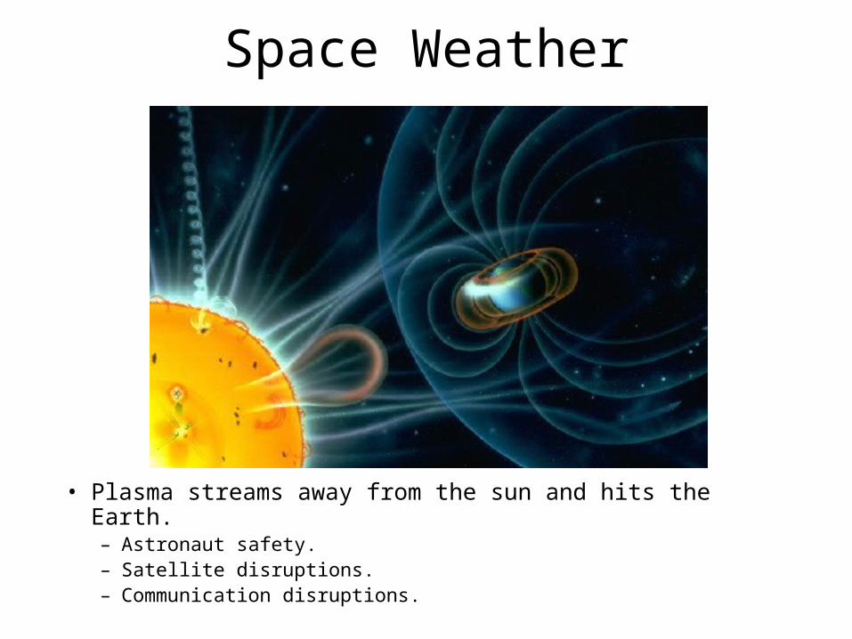
Space Weather

• Plasma streams away from the sun and hits the Earth.– Astronaut safety.– Satellite disruptions.– Communication disruptions.

Unlimited Clean Energy: Fusion

• Hydrogen gas must have:– Very high temperature and density.

• Plasma

Fusion 1: Tokamaks

• Compress and heat the plasma using magnetic fields.

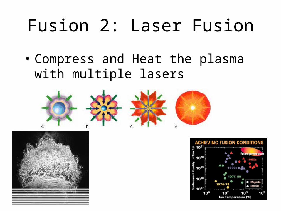
Fusion 2: Laser Fusion

• Compress and Heat the plasma with multiple lasers

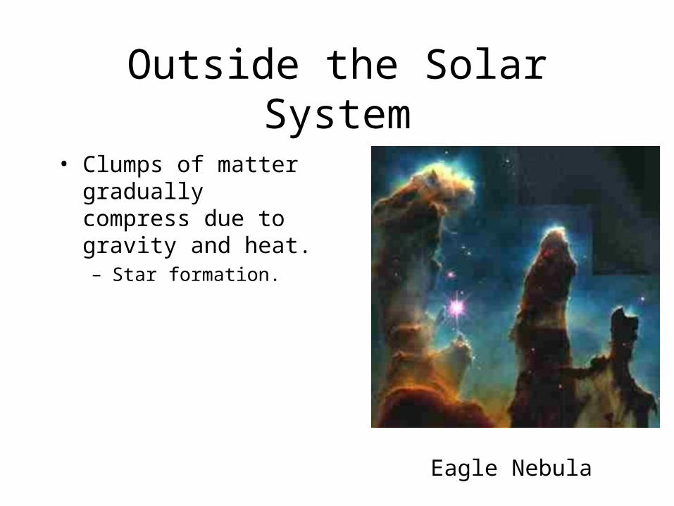
Outside the Solar System

• Clumps of matter gradually compress due to gravity and heat.– Star formation.

Eagle Nebula

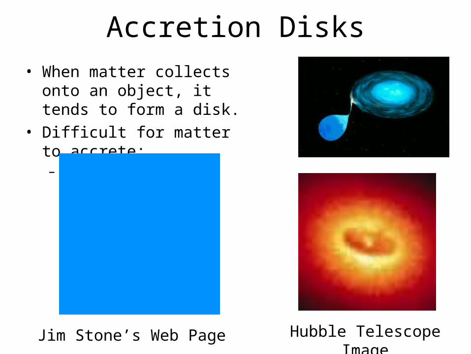
Accretion Disks• When matter collects onto an

object, it tends to form a disk.

• Difficult for matter to accrete:– Plasma Turbulence is key.

Hubble Telescope ImageJim Stone’s Web Page

The Wide Range of Plasmas

A Normal Gas (non-plasma)

• All dynamics is controlled through sound wave physics (Slinky Example).

Plasmas are More Complicated

N

S N

S

Magnetic Fields

• Wave a magnet around with a plasma in it and you will created wind!

• In fact, in the simplest type of plasmas, magnetic fields play an extremely important role.

Frozen-in Condition

• In a simple form of plasma, the plasma moves so that the magnetic flux through any surface is preserved.

Magnetic Field Waves

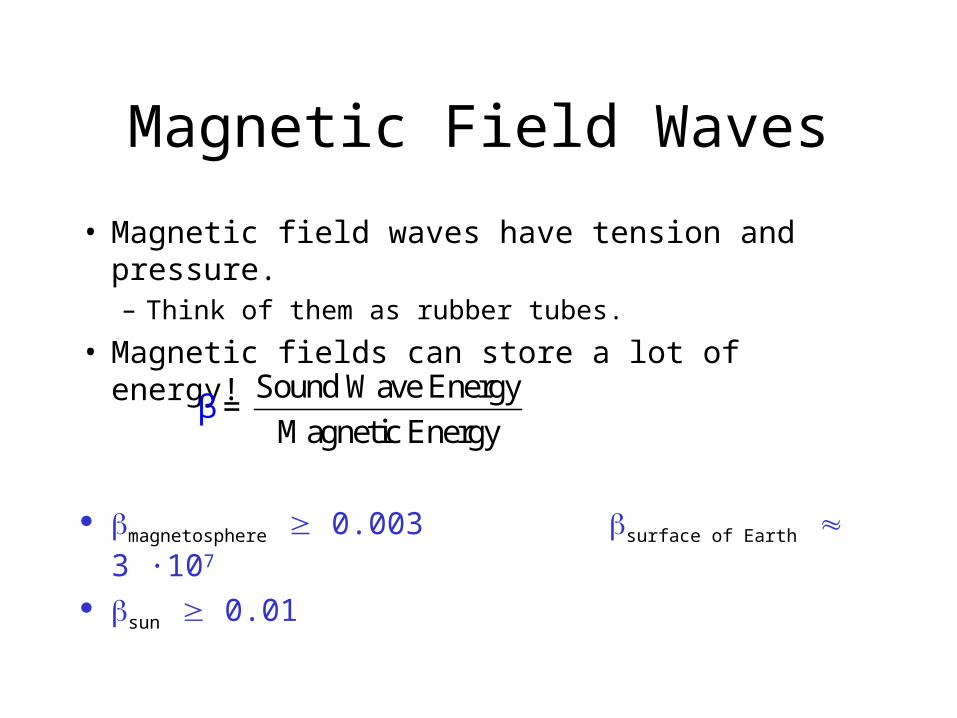
• Magnetic field waves have tension and pressure.– Think of them as rubber tubes.

• Magnetic fields can store a lot of energy!

magnetosphere 0.003 surface of Earth 3 ·107

sun 0.01

Sound Wave Energy =

Magnetic Eβ

nergy

Magnetic Fields: Rubber Tubes

Bi

Bfw

L

R

• Disparate scales: w << R << L

• Incompressible: Lw ~ R2

• Conservation of Magnetic Flux: Bf ~ (w/R) Bi

• Change in Magnetic Energy:

B energy density ~ B2/8Ef ~ (w/L) Ei << Ef

Magnetic Field Lines Can’t Break

=>

Everything Breaks

Eventually

Approximations

• Magnetic fields acting like rubber tubes assumes the slow plasma response.– Good for slow motions– Large scales

• Slinky• It will break:

– Fast Timescales/motions– Small lengths.

Field Lines Breaking: Reconnection

Vin

CA

Process breaking the frozen-in constraint determines the width of

the dissipation region,

Field Lines Breaking: Reconnection

Jz and Magnetic Field Lines

Y

X

What “Reconnection” Isn’t

Application – Solar Flares

Reconnection

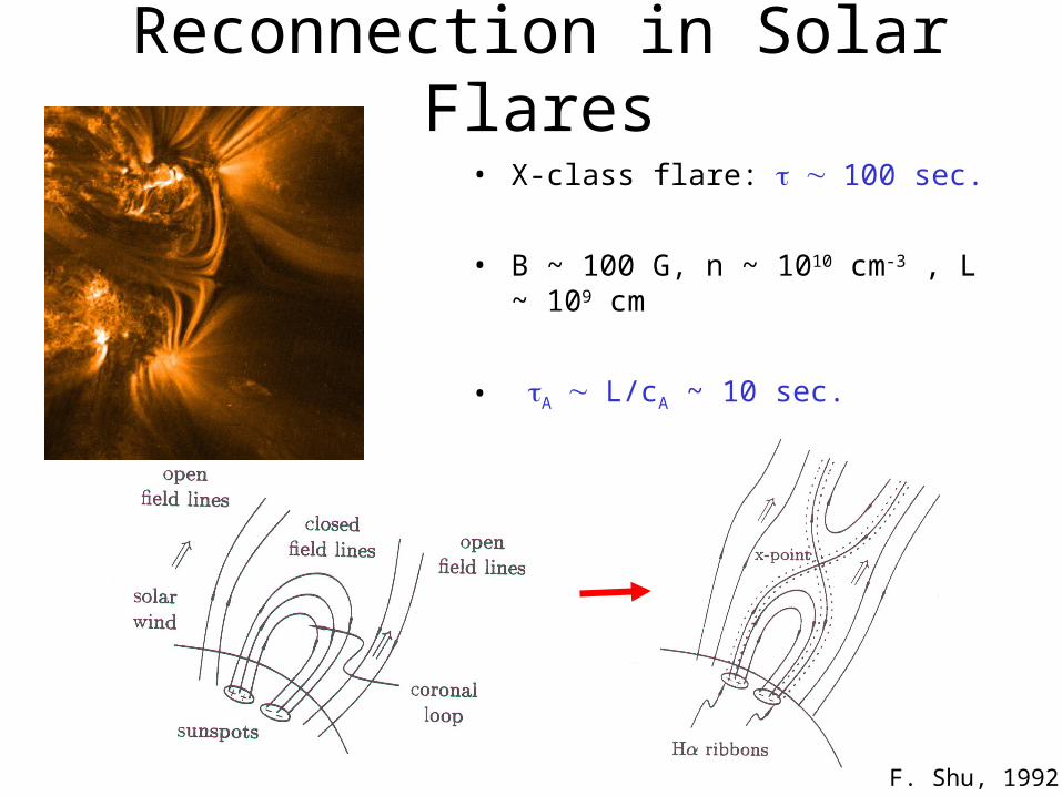
Reconnection in Solar Flares

F. Shu, 1992

• X-class flare: 100 sec.

• B ~ 100 G, n ~ 1010 cm-3 , L ~ 109 cm

• AL/cA ~ 10 sec.

Application - Magnetospheric Physics

ToSun

DaysideReconnection

MagnetotailReconnection

Part II: Simulating Reconnection

Reconnection is Hard

• Remember slinky?

• Now global (important) answers are strongly dependent on very fast/small timescales.

• If you have to worry about very small timescales, it makes the problem very hard.

Currently, Two Choices

• Macro Simulations:– Treat reconnection in a non-physical way.– Simulate Large Systems.

• Micro Simulations– Treat reconnection physically.– Simulate small idealized systems.

Our General Simulations

• Initial Value Problems– You give me the system initially, and I’ll tell

you how it will behave in the future.

A “Real” Plasma

• Individual charge particles (on board)

• Simply Calculate forces between each particle.– Problem: N total particles.– For each N particle, have to calculate force

from (N-1) particles.– Calculations per time step: N2. Prohibitively

expensive.

One Simplification: The Fluid Approximation

Fluid Approximation

• Break up plasma into infinitesmal cells.

• Define average properticies of each cell (fluid element)– density, velocity, temperature, etc.– Okay as long as sufficient particles per cell.

The Simplest Plasma Fluid: MHD

• Magnetohydrodynamics (MHD):

– Describes the slow, large scale behavior of plasmas.

• Now, very straightforward to solve numerically.

2

4 8i

dm n nT

dt

ct

n nt

c

B B BV

B E

V

VE B

Simulating Fluid Plasmas

• Define Fluid quantities on a grid cell.

• Dynamical equations tell how to step forward fluid quantities.

• Problem with Numerical MHD:– No reconnection in

equations.

– Reconnection at grid scale.

Grid cell

n,V,B known.

MHD Macro Simulations

• Courtesy of the University of Michigan group:– Remember that reconnection occurs only at grid

scale.

Non-MHD Micro Fluid Simulations

• Include smaller scale physics but still treat the system as a fluid.

Effective Gyration Radius

• Frozen-in constraint broken when scales of variation of B are the same size as the gyro-radius.

Electron gyroradius << Ion gyroradius

=> Dissipation region develops a 2-scale structure.

E

B

Electrons:

Ions:

Removing this Physics

VinCA

y

xz

X

Y

Hall Term No Hall Term

Out of Plane Currentme/mi = 1/25

Simulating Particles

• Still have N2 problem. How do we do it?

• Forces due to electric and magnetic fields.– Fields exist on grids => Fluid– Extrapolate to each particles location.

• Particles can be thought of as a Monte-Carlo simulation.

Simulating Kinetic Reconnection

• Finite Difference– Fluid quantities exist at grid

points.

• E,B treated as fluids always– Maxwell’s equations

• Two-Fluid– E,B,ions, electrons are fluid

• Kinetic Particle in Cell– E,B fluids– Ions and electrons are particles.– Stepping fluids: particle

quantities averaged to grid.– Stepping particles: Fluids

interpolated to particle position.

Grid cell

Macro-particle

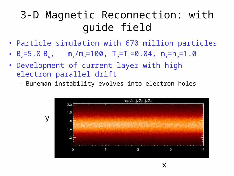
• Particle simulation with 670 million particles

• Bz=5.0 Bx, mi/me=100, Te=Ti=0.04, ni=ne=1.0

• Development of current layer with high electron parallel drift– Buneman instability evolves into electron holes

3-D Magnetic Reconnection: with guide field

y

x

Formation of Electron holes

• Intense electron beam generates Buneman instability– nonlinear evolution into “electron holes”

• localized regions of intense positive potential and associated anti-parallel electric field

x

z

Ez

Electron Holes• Localized region of positive potential in three space

dimensions– ion and electron dynamics essential

• different from structures studied by Omura, et al. 1996 and Goldman, et al. 1999 in which the ions played no role

– scale size Vd/pe in all directions

– drift speed ~Vd/3– dynamic structures (spontaneously form, grow and die)

• Drag Dz has complex spatial and temporal structure with positive and negative values

– quasilinear ideas fail badly

• Dz extends along separatrices at late time

• Dz fluctuates both positive and negative in time.

Electron drag due to scattering by parallel electric fields

y

x

The End