The Physics of Magnetic Reconnection

Reconnection: A Fundamental Process • What is Reconnection? • Conditions for Reconnection

Magnetospheric Reconnection and Convection • Steady vs. Unsteady • IMF and Geomagnetic Geometry

Physical Models & Simulations

Observations • Linking Reconnection to Aurora • Future Missions - When, Why, How?

EAS 4360/6360 16:1

Reading!!Baumjohann & Treumann, Chapter 5 !!Useful Resources !Space Physics Textbook, University of Oulu!http://www.oulu.fi/~spaceweb/textbook/merging.html Wikipedia’s Page http://en.wikipedia.org/wiki/Magnetic_reconnection !

EAS 4360/6360 16:2

The Physics of Magnetic Reconnection

Magnetic Reconnection or “Magnetic Merging”

“The process whereby magnetic field lines from different magnetic domains are spliced to one another, changing the overall topology of a magnetic field.”

(from Wikipedia)

Initial Reconnecting Final

EAS 4360/6360 16:3

What is Magnetic Reconnection?

Magnetic reconnection occurs throughout the Universe

Solar Flares and Coronal Mass Ejections: Magnetic fields on the Sun reconnect, ejecting huge, plasma filled loops into space.

EAS 4360/6360 16:4

What is Magnetic Reconnection?

EAS 4360/6360 16:5

What is Magnetic Reconnection? Magnetic reconnection occurs throughout the Universe

Solar Flares and Coronal Mass Ejections: Magnetic fields on the Sun reconnect, ejecting huge, plasma filled loops into space.

Magnetic reconnection occurs throughout the Universe Magnetopause Reconnection: The Interplanetary Magnetic Field (IMF) reconnects with the Earth’s magnetic field, at the magnetopause (the outer boundary of the magnetosphere). Also called “Dayside Merging”

Geomagnetic Field IMF

(southward)

EAS 4360/6360 16:6

What is Magnetic Reconnection?

Magnetic reconnection occurs throughout the Universe

Magnetotail Reconnection: Two oppositely directed “tail” fields (“Northern” and “Southern”) reconnect, often leading to an explosive release of energy called a “substorm”.

N Tail Field

S Tail Field

EAS 4360/6360 16:7

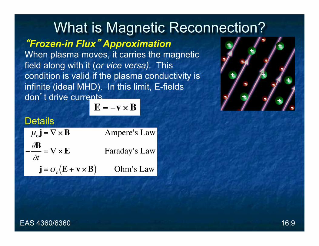
What is Magnetic Reconnection?

“Frozen-in Flux” Approximation When plasma moves, it carries the magnetic field along with it (or vice versa). This condition is valid if the plasma conductivity is infinite (ideal MHD). In this limit, E-fields don’t drive currents.

EAS 4360/6360 16:8

What is Magnetic Reconnection?

€

E = −v ×B

€

µoj =∇ ×B Ampere's Law

−∂B∂t

=∇ ×E Faraday's Law

j =σ o E + v ×B( ) Ohm's Law

Details

“Frozen-in Flux” Approximation When plasma moves, it carries the magnetic field along with it (or vice versa). This condition is valid if the plasma conductivity is infinite (ideal MHD). In this limit, E-fields don’t drive currents.

EAS 4360/6360 16:9

What is Magnetic Reconnection?

€

E = −v ×B

€

E = −v ×B +jσ o

Full Ohm’s Law

€

µoj =∇ ×B Ampere's Law

−∂B∂t

=∇ ×E Faraday's Law

j =σ o E + v ×B( ) Ohm's Law

Details

“Frozen-in Flux” Approximation When plasma moves, it carries the magnetic field along with it (or vice versa). This condition is valid if the plasma conductivity is infinite (ideal MHD). In this limit, E-fields don’t drive currents.

EAS 4360/6360 16:10

What is Magnetic Reconnection?

€

E = −v ×B

€

∂B∂t

=∇ × v ×B( ) + 1σ oµo

∇2B

€

E = −v ×B +jσ o

Full Ohm’s Law

€

µoj =∇ ×B Ampere's Law

−∂B∂t

=∇ ×E Faraday's Law

j =σ o E + v ×B( ) Ohm's Law

Details

“Frozen-in Flux” Approximation When plasma moves, it carries the magnetic field along with it (or vice versa). This condition is valid if the plasma conductivity is infinite (ideal MHD). In this limit, E-fields don’t drive currents.

EAS 4360/6360 16:11

What is Magnetic Reconnection?

€

E = −v ×B

Standard “Diffusion Equation” €

∂B∂t

=∇ × v ×B( ) + 1σ oµo

∇2B

€

E = −v ×B +jσ o

Full Ohm’s Law

€

µoj =∇ ×B Ampere's Law

−∂B∂t

=∇ ×E Faraday's Law

j =σ o E + v ×B( ) Ohm's Law

Details

“Frozen-in Flux” Approximation When plasma moves, it carries the magnetic field along with it (or vice versa). This condition is valid if the plasma conductivity is infinite (ideal MHD). In this limit, E-fields don’t drive currents.

EAS 4360/6360 16:12

What is Magnetic Reconnection?

€

E = −v ×B

€

∂Q∂t

= K∇2Q“Frozen-in Flux”

Term “Diffusion”

Term e.g. Heat Diffusion

Magnetic Diffusivity Coefficient of “diffusion term”

€

∂B∂t

=∇ × v ×B( ) + 1σµ0

∇2B

€

Dm ≡1

σ oµoMagnetic Reynolds Number * Ratio of “frozen-in” and “diffusion” terms. Measure of magnetic field line “slippage”

* RM is very large for typical space plasmas (e.g., in magnetosphere, L ~ few RE and v ~ 100 km/s… RM = 1011)

* Condition for reconnection: RM ~ 1 or less.

€

RM ≡ "FROZEN-IN""DIFFUSION"

=vLBDm

=σ oµovLB

“Frozen-in Flux” “Diffusion”

EAS 4360/6360 16:13

How ‘Ideal’ is the Plasma?

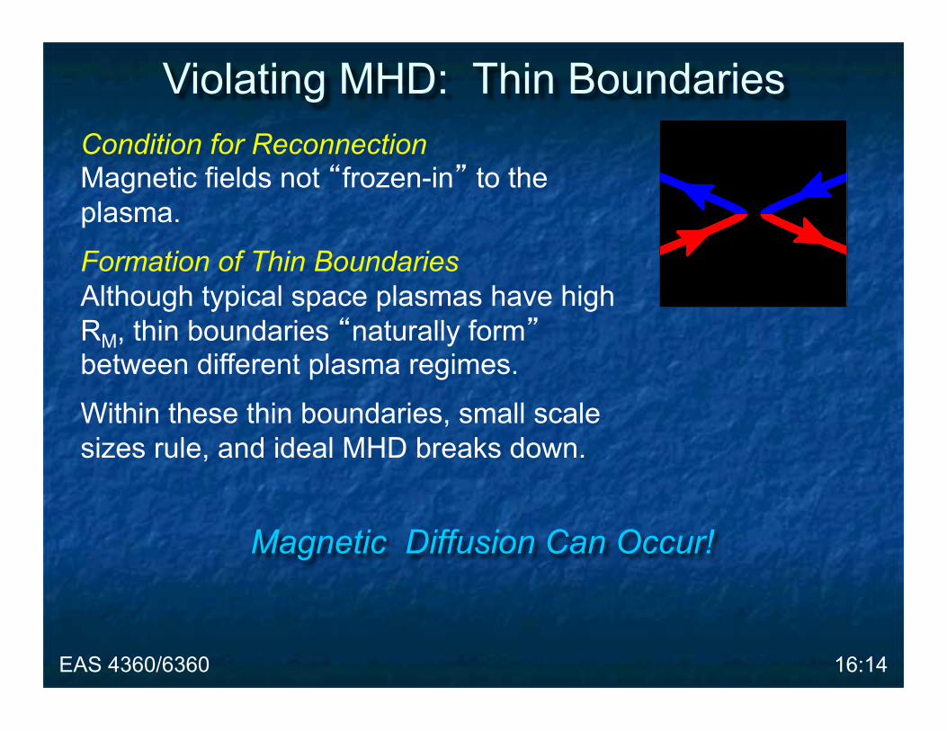
Condition for Reconnection Magnetic fields not “frozen-in” to the plasma.

Formation of Thin Boundaries Although typical space plasmas have high RM, thin boundaries “naturally form” between different plasma regimes.

Within these thin boundaries, small scale sizes rule, and ideal MHD breaks down.

EAS 4360/6360 16:14

Violating MHD: Thin Boundaries

Magnetic Diffusion Can Occur!

Current Sheets: Thin Boundaries in the Magnetosphere A dipole field is curl-free. But the real magnetosphere does have a curl--thus there are current sheets needed to maintain its configuration. These current sheets result “naturally” from the solar wind-magnetosphere interaction.

EAS 4360/6360 16:15

Current Sheets

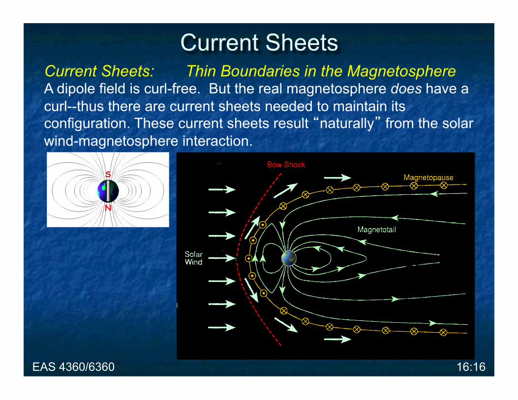
Current Sheets: Thin Boundaries in the Magnetosphere A dipole field is curl-free. But the real magnetosphere does have a curl--thus there are current sheets needed to maintain its configuration. These current sheets result “naturally” from the solar wind-magnetosphere interaction.

EAS 4360/6360 16:16

Current Sheets

Current Sheets: Thin Boundaries in the Magnetosphere A dipole field is curl-free. But the real magnetosphere does have a curl--thus there are current sheets needed to maintain its configuration. These current sheets result “naturally” from the solar wind-magnetosphere interaction.

EAS 4360/6360 16:17

Current Sheets

Current Sheets: Thin Boundaries in the Magnetosphere A dipole field is curl-free. But the real magnetosphere does have a curl--thus there are current sheets needed to maintain its configuration. These current sheets result “naturally” from the solar wind-magnetosphere interaction.

EAS 4360/6360 16:18

Current Sheets

The Diffusion Region and “X-Type Neutral Line”

• Vertical inflow brings oppositely directed B together: Current Sheet.

• In small diffusion region, ideal MHD breaks down (RM small).

• With MHD relaxed, B-field can reconnect (X-Line)

• Horizontal outflow carries new B-field topology away.

X-Line At center of

diffusion region

EAS 4360/6360 16:19

Concepts of Reconnection

The “Dungey Cycle” Dungey [1961] proposed that reconnection drove plasma convection (ExB drift) in the magnetosphere.

2 locations: • Dayside of the magnetosphere • At an X-line in the magnetotail

Except at the reconnection sites, magnetic field lines “frozen in”, meaning entire flux tube moves, even in ionosphere.

magnetotail reconnection

dayside reconnection Dayside Reconnection Rate

Drives entire process

EAS 4360/6360 16:20

Magnetospheric Reconnection

The “Dungey Cycle” Dungey [1961] proposed that reconnection drove plasma convection (ExB drift) in the magnetosphere.

2 locations: • Dayside of the magnetosphere • At an X-line in the magnetotail

Except at the reconnection sites, magnetic field lines “frozen in”, meaning entire flux tube moves, even in ionosphere.

Dayside Reconnection Rate Drives entire process

EAS 4360/6360 16:21

Magnetospheric Reconnection

The “Dungey Cycle” Dungey [1961] proposed that reconnection drove plasma convection (ExB drift) in the magnetosphere.

2 locations: • Dayside of the magnetosphere • At an X-line in the magnetotail

Except at the reconnection sites, magnetic field lines “frozen in”, meaning entire flux tube moves, even in ionosphere.

EAS 4360/6360 16:22

Magnetospheric Reconnection

Ionosphere: “Two-Cell” Convection

The “Dungey Cycle” Dungey [1961] proposed that reconnection drove plasma convection (ExB drift) in the magnetosphere.

2 locations: • Dayside of the magnetosphere • At an X-line in the magnetotail

Except at the reconnection sites, magnetic field lines “frozen in”, meaning entire flux tube moves, even in ionosphere.

EAS 4360/6360 16:23

Magnetospheric Reconnection

Ionosphere: “Two-Cell” Convection

Dayside Reconnection Rate Drives entire process

Magnetic Flux Transfer Reconnection removes magnetic flux from the dayside and brings it to the nightside (i.e., magnetotail).

Magnetopause Erosion Note that just after reconnection, the outermost closed field line (i.e., the magnetopause) has moved inward.

In the simple schematic picture to the right, the magnetopause moves from:

Larger magnetopause (before reconnection)

to Smaller magnetopause

(after reconnection)

  (add this to dynamic pressure compression of m’pause!)

EAS 4360/6360 16:24

Magnetopause ‘Erosion’

Open Field Lines After dayside reconnection, magnetic field lines connect the ionosphere directly to the solar wind. These are called “open field lines”.

Polar Cap The portion of the ionosphere containing open field lines is called the “polar cap.”

The Aurora The lower-latitude edge of the polar cap is often the site of aurora. The aurora are caused by charged particles, funneled down by the magnetic field, raining down (“precipitating”) into the upper atmosphere. Collisions with the precipitating particles cause the atmosphere to fluoresce.

Aurora

EAS 4360/6360 16:25

Magnetopause ‘Erosion’

Aurora

EAS 4360/6360 16:26

Magnetopause ‘Erosion’

The Aurora The lower-latitude edge of the polar cap is often the site of aurora. The aurora are caused by charged particles, funneled down by the magnetic field, raining down (“precipitating”) into the upper atmosphere. Collisions with the precipitating particles cause the atmosphere to fluoresce.

IMF Clock Angle Dayside Reconnection depends strongly upon the angle between the Interplanetary Magnetic Field (IMF) and the (Earth’s) geomagnetic field.

This angle is called “IMF Clock angle”.

The IMF clock angle determines the location of the open-closed boundary.

The Bz Effect

When Bz < 0, Reconnection erodes the magnetopause, causing the auroral oval to move

lower in latitude.

Earth’s Field

IMF Bz < 0

Earth’s Field

IMF By

The By Effect

The By polarity shifts the auroral oval either

toward dawn or toward dusk.

EAS 4360/6360 16:27

Southward IMF

The By Effect The “Dawn-Dusk”

component can skew the reconnection geometry.

The Bz Effect

When Bz < 0, Reconnection erodes the magnetopause, causing the auroral oval to move

lower in latitude.

Earth’s Field

IMF Bz < 0

Earth’s Field

IMF By

The By Effect

The By polarity shifts the auroral oval either

toward dawn or toward dusk.

EAS 4360/6360 16:28

Southward IMF

IMF “Southward”? The Earth’s magnetic dipole is not exactly aligned with the spin axis, so that as the Earth rotates, the magnetic dipole “wobbles”, even if the IMF direction is constant.

EAS 4360/6360 16:29

Tilt of the Magnetic Dipole

Tsyganenko Model

Steady Convection Magnetic flux is removed from the dayside and delivered to the nightside. But magnetotail reconnection then carries that magnetic flux back to the dayside. If the rates of dayside reconnection and magnetotail reconnection are the same, then this will set up a “steady” convection--so long as the IMF is steady!

EAS 4360/6360 16:30

Magnetospheric Convection

Unsteady Convection In truth, steady convection may not be all that common. If the rates of dayside reconnection and magnetotail reconnection are not equal, then this will set up “unsteady” convection.

Substorms are an example of unsteady reconnection & convection.

If the IMF is not steady, convection will not be steady.

EAS 4360/6360 16:31

Magnetospheric Convection

Not Just Southward IMF Even when the IMF is “northward”, reconnection can still take place at the magnetopause. The northward IMF can be oppositely directed to magnetic fields in the high- latitude “lobe” regions.

Lobe reconnection is probably less common, and much less efficient at transferring energy to the magnetosphere.

EAS 4360/6360 16:32

‘Lobe’ Reconnection

The Diffusion Region and “X-Type Neutral Line”

Physical Process that was poorly understood at first (delayed acceptance)

X-Line At center of

diffusion region

EAS 4360/6360 16:33

Concept of Reconnection

X-Line geometry & configuration

Large Diffusion Region (2L by 2l)

Symmetrical (Simple) (1)  Uniform electric field

(2)  Incompressible flow

(3)  Mass conservation

(4)  Mass flux

(5)  Conserve Energy

Sweet-Parker Solution

€

E = EeY

€

ρi = ρo = ρ

€

−2ui2l

+2uo2L

= 0 ⇒ uiL = uol

€

S = E ×H =E Bi

µ0

=ui Bi

2

µ0

IN : Electromagnetic Power / area

PMECH = 12 ρ ui( ) uo

2 − ui2( ) OUT: Mechanical Power / area€

ρ ui mass / area / time

EAS 4360/6360 16:34

Reconnection Rate: Sweet-Parker

Infinitessimal size diffusion region

Diffusion region generates standing slow-mode shock waves

Presence of shock waves speeds up reconnection rate.

Petschek Solution (1964)

Standing Shock Shock formed by a stationary object in a

super-“sonic” flow. The shock stays in the same position.

EAS 4360/6360 16:35

Reconnection Rate: Petschek

Add fast mode shocks 2 sets of shocks that divert

initial flow direction. Locations of fast mode

shocks determined by macroscopic plasma conditions

Sonnerup Solution (1970)

Macroscopic Determination of Reconnection Priest and Forbes (1986) solution demonstrates that

reconnection rate determined outside diffusion region, by global plasma parameters and scale sizes.

EAS 4360/6360 16:36

Reconnection Rate: Sonnerup

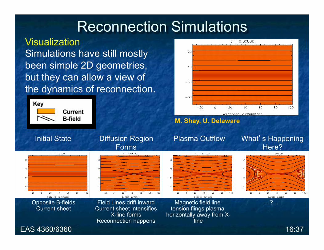
Visualization Simulations have still mostly been simple 2D geometries, but they can allow a view of the dynamics of reconnection.

M. Shay, U. Delaware

Initial State Diffusion Region Forms

Plasma Outflow What’s Happening Here?

Opposite B-fields Current sheet

Field Lines drift inward Current sheet intensifies

X-line forms Reconnection happens

Magnetic field line tension flings plasma

horizontally away from X-line

…?…

Key Current B-field

EAS 4360/6360 16:37

Reconnection Simulations

Visualization Simulations have still mostly been simple 2D geometries, but they can allow a view of the dynamics of reconnection.

M. Shay, U. Delaware

Initial State Diffusion Region Forms

Plasma Outflow Boundary Contamination

Opposite B-fields Current sheet

Field Lines drift inward Current sheet intensifies

X-line forms Reconnection happens

Magnetic field line tension flings plasma

horizontally away from X-line

Oops! Outflow bumps into boundary conditions.

Simulations have practical limitations.

Key Current B-field

EAS 4360/6360 16:38

Reconnection Simulations

More Complicated Dynamics Computational solutions can treat some complicated dynamics and physics that are difficult to include in analytical models.

McClymont & Craig (1996)

Compression & Rarefaction

Inflow causes rarefaction. Outflow causes compression.

Current sheet formation is from the “ends inward”

Key Density B-field

Current Sheet is Formed

High density reached at center of current sheet. Low

density “holes” in inflow lobes.

Outflow: plasma jets

Mass is squirted out of the ends of the current sheet,

streams along separatrices. Very thin current sheet!

EAS 4360/6360 16:39

Reconnection Simulations

Tanuma & Shibata (2005)

Current Sheet Collapse

The initial part of the simulation follows the classic current sheet

development.

“Internal” Shocks

Complicated shock waves develop inside the

reconnection region.

Plasma Instability

The “tearing mode” instability develops,

producing magnetic & pressure “islands”.

More Complicated Physics Computational solutions can treat some complicated dynamics and physics that are difficult to include in analytical models.

EAS 4360/6360 16:40

Reconnection Simulations

Kivelson & Russell, Fig 9.23

Magnetopause Crossing ISEE 2 spacecraft: Outward magnetopause crossing, 12 Aug 1978.

Indirect signature of reconnection Increased V, Vy, N

EAS 4360/6360 16:41

Observations

Kivelson & Russell, Fig 9.23

Magnetopause Crossing ISEE 2 spacecraft: Outward magnetopause crossing, 12 Aug 1978.

Indirect signature of reconnection Increased V, Vy, N

EAS 4360/6360 16:42

Observations

Remote Sensing: The Aurora Auroral imagers see global picture of aurora.

The Aurora The aurora are caused by charged particles, funneled down by the magnetic field, raining down (“precipitating”) into the upper atmosphere. Collisions with the precipitating particles cause the atmosphere to fluoresce.

EAS 4360/6360 16:43

Observations

Substorm Onset Beginning of auroral signatures associated with substorms.

Indirect signature of MAGNETOTAIL reconnection Particles from reconnection site precipitate into the atmosphere.

Onset Expansion Westward Surge Recovery

Auroral Substorm

EAS 4360/6360 16:44

Observations

Proton Cusp Aurora (Frey et al., 2002) IMAGE auroral imager sees “spot” in cusp.

Indirect signature of DAYSIDE reconnection Particles from reconnection site funneled to upper atmosphere. Signature appears during Southward IMF

Frey et al. [2003] EAS 4360/6360 16:45

Observations

Conjugate Cusp Aurora (Ostgaard et al., 2005) IMAGE auroral imager sees conjugate “spots” in cusp.

Indirect signature of DAYSIDE reconnection geometry Conjugate spots consistent with reconnection hypothesis

Ostgaard et al. [2005]

EAS 4360/6360 16:46

Observations

X-Ray Spot (Ostgaard et al., 2006)

Polar PIXIE data Bright X-ray energy spot

Magnetic Mapping to the Geotail

Flow Reversal at Mapped Location of Spot

Plasma data from Cluster

A B

+Vx - Vx

EAS 4360/6360 16:47

Observations

What’s Left to Learn? Plenty 1.  What are the kinetic processes responsible for

collisionless reconnection? 2.  How is reconnection initiated? 3.  Where does reconnection occur in the

magnetopause and in the magnetotail? 4.  What influences the location of reconnection? 5.  How does reconnection vary with time, and

what factors influence its temporal behavior? 6.  How do FTEs and plasmoids form and

evolve? 7.  What is the role of induction E-fields and

wave-particle interactions in acceleration processes?

8.  What are the properties and processes associated with magnetospheric turbulence?

EAS 4360/6360 16:48

Open Questions

Magnetospheric Multiscale (MMS) Explore Reconnection… 4 spacecraft, Launch 2014

Time History of Events and Macroscale Interactions during Substorms (THEMIS) Substorm Timing… 5 spacecraft, LAUNCHED 17 Feb 2007 3 x 10 RE + 20 RE + 30 RE

EAS 4360/6360 16:49

Future Missions

Reading: Read the paper ‘Continuous magnetic reconnection at Earth’s Magnetopause’ by Frey, Phan, Fuselier, and Mende (Nature, 2003) (to be handed out on Friday) Write: Paragraph Summary of the paper for discussion on Wednesday

EAS 4360/6360 16:50

Assignment