ROOTS OF EQUATIONS

BRACKETING METHODS

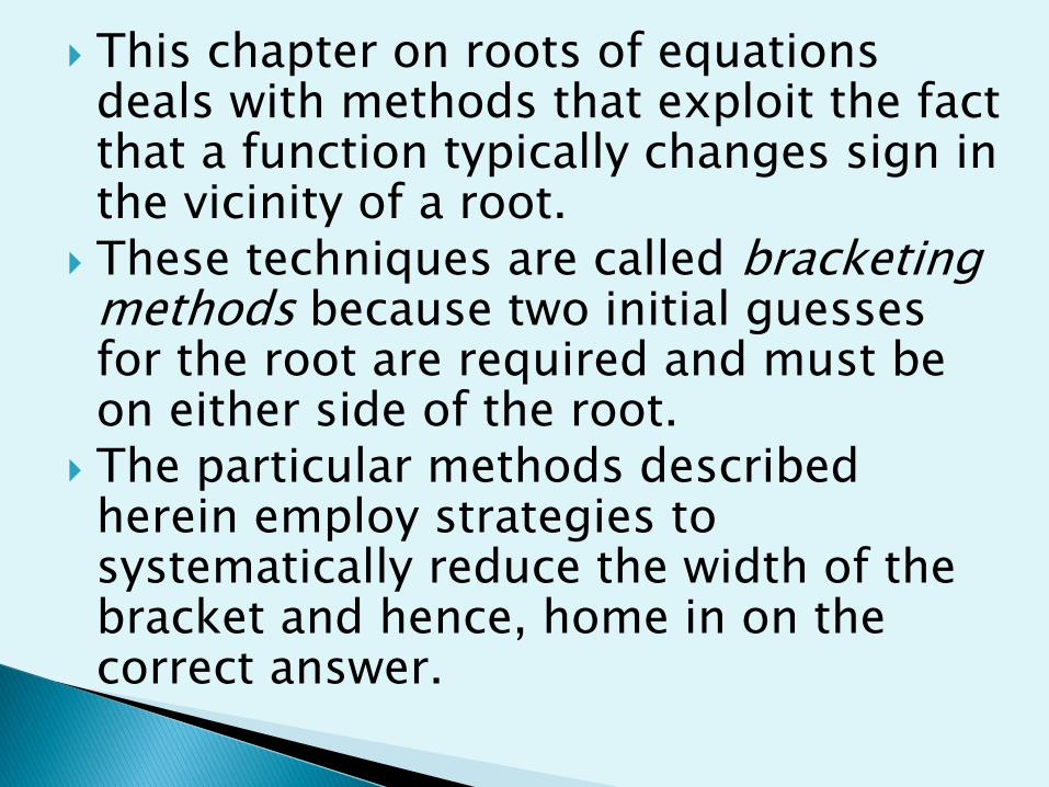
This chapter on roots of equations deals with methods that exploit the fact that a function typically changes sign in the vicinity of a root.

These techniques are called bracketing methods because two initial guesses for the root are required and must be on either side of the root.

The particular methods described herein employ strategies to systematically reduce the width of the bracket and hence, home in on the correct answer.

Numerical Methods – these are techniques by

which engineering problems are solved by

basic arithmetic operations, which are

normally long and tedious (i.e. iterative /

repetitive)

TYPES OF EQUATION

1.Polynomial or Algebraic Equations

Theory: Every equation f(x) = 0 of degree n has most n distinct roots. If the equation has a + bi as a root, then it has a –bi also as a root.

Signs of the roots

Let f(x) have real coefficients and be arranged in descending powers of x. Then, if two successive terms differ in sign, there is said to be a variation of sign. In counting the variation, zero coefficients or missing powers of x are disregarded.

If f(x) =x4-5x3+6x2-9 : _____variations of sign

If f(x) = 2x4+5x2-4x-1 : ____variations of sign

DESCARTES’ RULE OF SIGNS

If f(x) is a polynomial with real coefficients, the number of positive roots of the equation f(x)=0 cannot exceed the number of variation of sign in f(x), and, in any case, differs from the number of variations by an even integer.

To determine the number of negative roots

f(x)=0 , determine the number of positive

roots of f(-x)=0 .

Example: Determine the number of positive and negative

roots of the equation

a) f(x) = 2x4 + 5x2 - 4x -1

b) f(x) = 2x5 – 3x4 + 2x - 5

A simple method for obtaining an estimate of the root of the equation f(x)=0 is to make a plot of the function and observe where it crosses the x axis.

x

y

Root

Illustration of a number of general ways that a root may occur in an interval prescribed by a lower bound xl and an upper bound xu.

Parts (a) and (c) indicate that if both f(xl) and f(xu) have the same sign, either there will be no roots or there will be an even number of roots within the interval. Figure 5.2

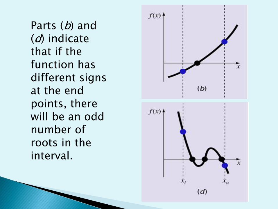
Parts (b) and (d) indicate that if the function has different signs at the end points, there will be an odd number of roots in the interval.

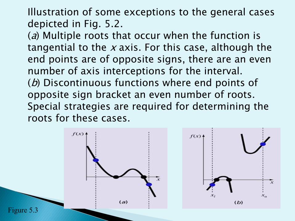
Illustration of some exceptions to the general cases depicted in Fig. 5.2.

(a) Multiple roots that occur when the function is tangential to the x axis. For this case, although the end points are of opposite signs, there are an even number of axis interceptions for the interval.

(b) Discontinuous functions where end points of opposite sign bracket an even number of roots. Special strategies are required for determining the roots for these cases.

Figure 5.3

In general, if f(x) is real and continuous in the interval from xl to xu and f(xl) and f(xu) have opposite signs then there is at least one real root between xl and xu

The bisection method is one type of an incremental search method in which the interval is always divided in half.

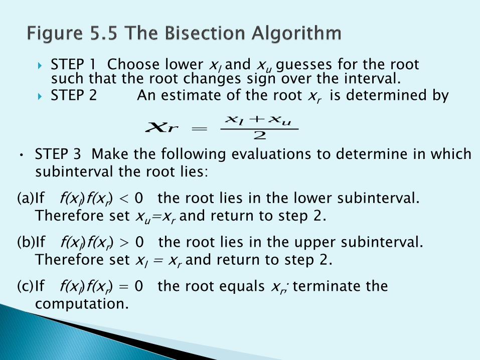
STEP 1 Choose lower xl and xu guesses for the root such that the root changes sign over the interval.

STEP 2 An estimate of the root xr is determined by

2

ul xxrx

• STEP 3 Make the following evaluations to determine in which subinterval the root lies:

(a)If f(xl)f(xr) < 0 the root lies in the lower subinterval. Therefore set xu=xr and return to step 2.

(b)If f(xl)f(xr) > 0 the root lies in the upper subinterval. Therefore set xl = xr and return to step 2.

(c)If f(xl)f(xr) = 0 the root equals xr; terminate the computation.

A graphical depiction of the bisection method.

Figure 5.6

%100new

r

old

r

new

ra

x

xx

When εa becomes less than a pre-specified stopping

criterion εs, the computation is terminated.

Table form:

n xl f(xl) xu Xr f(xr) f(xl)f(xr)

1

2

Example: Find the positive root of f(x) =4x3-6x2+7x-2.3

(use 4 decimal places), use x =-5, -4, -3…

A shortcoming of the bisection method is that it does not take into account the magnitudes of f(xl) and f(xu).

For example, if f(xl) is much closer to zero than f(xu), it is likely that the root is closer to xl than to xu

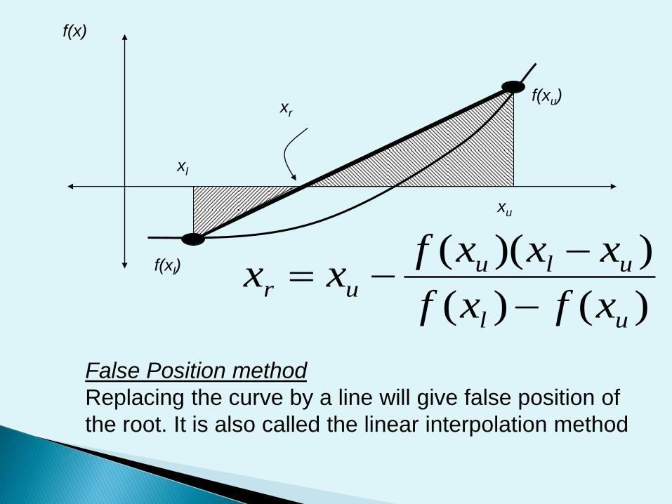
An alternative method that exploits this graphical insight is to join f(xl) and f(xu) by a straight line. The intersection of this line with the x-axis represents an improved estimate of the root.

)()(

))((

ul

uluur

xfxf

xxxfxx

f(x)

f(xu)

xu

f(xl)

xl

xr

False Position method

Replacing the curve by a line will give false position of

the root. It is also called the linear interpolation method

One way to mitigate the “one-sided” nature of false position is to have the algorithm detect when one of the bounds is stuck. If this occurs, the function value at the stagnant bound can be divided in half. This is called the modified false-position method.

Example:

Determine the real roots of f(x)=-13-20x+19x2 – 3x2 using the Regula Falsi method to 3 decimal places. Use xl = -1 and xu = 0.