Numerical Methods for High Speed Vehicle Dynamic...
36
Numerical Methods for High Speed Vehicle Dynamic Simulation Edward J. Haug Dan Negrut* Radu Serban** Dario Solis Automotive Research Center and NSF Center for Virtual Proving Ground Simulation NADS and Simulation Center The University of Iowa Iowa City, Iowa 52242 April 30, 1999 -------------------------- *Presently Senior Development Engineer, Mechanical Dynamics, Inc., 2301 Commonwealth Blvd., Ann Arbor, MI 48105 **Presently Postgraduate Researcher, Computational Science and Engineering Program, Department of Mechanical and Environmental Engineering, University of California at Santa Barbara, Santa Barbara, CA 93106
Transcript of Numerical Methods for High Speed Vehicle Dynamic...

Numerical Methods for High Speed Vehicle Dynamic Simulation
Edward J. Haug
Dan Negrut*
Radu Serban**
Dario Solis
Automotive Research Center
and
NSF Center for Virtual Proving Ground Simulation
NADS and Simulation Center
The University of Iowa
Iowa City, Iowa 52242
April 30, 1999
--------------------------
*Presently Senior Development Engineer, Mechanical Dynamics, Inc., 2301 Commonwealth
Blvd., Ann Arbor, MI 48105
**Presently Postgraduate Researcher, Computational Science and Engineering Program,
Department of Mechanical and Environmental Engineering, University of California at Santa
Barbara, Santa Barbara, CA 93106

2
Abstract
Recent developments in numerical methods for high speed vehicle dynamic simulation in
the multi-university Automotive Research Center sponsored by the U.S. Army Tank-Automotive
Research, Development, and Engineering Center are summarized and illustrated. The prior
state-of-the-art is reviewed and computational developments focusing on both computer-aided
engineering applications with stiff equations and driver-in-the-loop real-time vehicle system
simulation are presented. To illustrate gains achieved in computational efficiency and reliability,
realistic handling models of the Army High Mobility Multi-Purpose Wheeled Vehicle are
simulated and compared to results obtained using previous methods. A demonstration of two
orders of magnitude speed-up for stiff vehicle models characteristic of those employed by
vehicle developers in computer-aided engineering is presented. Achievement of real-time
simulation on computing platforms integral to emerging driving simulators that are establishing
new capabilities for virtual proving ground simulation is presented.
1. Prior State-of-the-Art
Prior to the mid 1990s, a decade of development in the technology of multibody dynamic
simulation had advanced the state-of-the-art to the point that significant capabilities were
available, but significant limitations remained, as follows:
(1) Real-time simulation for emerging driver-in-the-loop simulators was feasible with
models accounting for up to 15 Hz frequency response (wheel hop frequency), using either
optimized symbolic (Wehage, Belczynski, 1992; Schiehlen, 1994) or complex recursive(Bae,
Haug, 1987a,b) formulations.
Simplified models with special formulations were required to achieve real-time
simulation, which were generally incompatible with computer-aided engineering (CAE) tools

3
such as DADS and ADAMS that are used in engineering design. Modeling incompatibilities that
resulted required that two distinct, generally incompatible, sets of models be used for driver-in-
the-loop real-time simulation to determine duty cycles and CAE analysis in design for subsystem
integrity and system performance.
(2) Reliable and accurate numerical integration of the differential-algebraic equations
(DAE) of multibody dynamics was possible only with explicit predictor-corrector methods,
which had significant difficulty with stiff models of vehicle systems that routinely arise in
engineering design.
The engineering community had no robust implicit numerical integration algorithms to
reliably carry out dynamic analysis of stiff differential-algebraic systems (Hairer, Wanner, 1996)
arising in practice. The implementation of implicit integrators (Hairer, Wanner, 1996) requires
calculation of a derivative of the equations of motion, for numerical solution of the discretized
equations. This implies the need for the derivative of all mass and force quantities, as well as
three derivatives of constraint expressions. Except for the highly inefficient alternative of
numerical differentiation, no practical means of obtaining these derivatives was available.
(3) High frequency vehicle subsystem response characteristics that are important in driver-
vehicle interaction could only be approximately modeled in achieving real-time performance.
High fidelity modeling of vehicle subsystems such as tires, headway control devices,
hybrid-electric powertrains, and a host of the emerging actively controlled devices appearing in
modern vehicles was not possible in real-time. As a result, often unsatisfactory simplified
models were used in real-time dynamic simulation.
(4) Computational environments for multibody dynamic simulation were either
nonexistent, or integrated into proprietary software such as ADAMS and DADS.

4
No modular software environments were available for creating, testing, and
implementing new algorithms and methods to overcome the difficulties outlined above. The
enormous number of formulation and computational alternatives that must be systematically
investigated to create fundamentally new methods to overcome the foregoing limitations can
only be effectively assessed in an integrated computational environment.
2. Scope of High Speed Dynamic Simulation Developments Addressed
High speed dynamic simulation research supported by the Army and the National Science
Foundation during the period 1994 to1998 focused on overcoming limitations in the four areas outlined
above. Upgrades being made in Tank and Automotive Research and Development Center soldier- and
hardware-in-the-loop simulators and US Department of Transportation development of the National
Advanced Driving Simulator (NADS) motivated research aimed at achieving real-time simulation, in
order to realize the potential for fundamental new virtual proving ground capabilities. The goal was to
support both human factors analysis and vehicle duty cycle determination and their integration with CAE
tools and technologies. The principal developments that resulted are summarized in more detail in the
body of the paper. A computational environment created to support the research reported in this paper is
briefly outlined in this section.
Starting from a vehicle model generated in formulations based on Cartesian coordinates
used in DADS, a general purpose computational environment has been created to support a
broad range of mutlibody mechanical analyses. Applications supported include explicit and
implicit numerical integration of the DAE of motion for vehicle system design, as well as real-
time simulation of vehicle systems for use in emerging vehicle driving simulators. The core of
this computational environment is shown in Fig. 1, comprising six basic tools developed in an
environment supporting both design level fidelity simulation and real-time simulation for

5
hardware- and operator-in-the-loop driving simulation. All developments presented in this paper
were implemented and tested in this environment.
Figure 1. Vehicle Multibody Dynamics Computational Environment
In order to assess the benefits of developments summarized in this paper, a realistic
handling model of the Army’s high mobility multipurpose wheeled vehicle (HMMWV) shown in
Fig. 2 is used as a test problem. The fourteen-body model of this vehicle adopted for test and
evaluation is shown in Fig. 3. It consists of four independent suspension subsystems, each with a
wheel spindle body, connected by spherical joints to a pair of control arms, which are in turn
connected to the chassis via rotational joints. Each wheel assembly is connected to the chassis or
to a steering rack using a tie rod, modeled as a distance constraint. Excluding the steering degree
of freedom, which is specified as an input, this model has 10 degrees of freedom. The kinematics
model using Cartesian coordinates employs a total of 98 generalized coordinates, subject to 88
nonlinear kinematic constraint equations. Force elements acting in the model, not shown in Fig.
3, include suspension spring and shock absorber elements and tire force elements.
Model Synthesis
Derivative Computation
Topology-BasedLinear Solvers
Globally Independent Generalized Coordinates
Dual-Rate Integration forSubsystem Simulation
Real-Time,High Fidelity,
Vehicle Simulation
Stable and EfficientImplicit Integrators
for Stiff Vehicle Models

6
Figure 2. U.S. Army High Mobility Multipurpose Wheeled Vehicle (HMMWV)
Figure 3. Fourteen-Body Model of HMMWV
In this paper, q = q1, q2, ..., q n[ ]T denotes the vector of generalized coordinates that define
the state of a multibody system (Haug, 1989). The generalized coordinates are Cartesian
position coordinates and orientation Euler parameters of body centroidal reference frames.

7
Joints connecting the bodies of a mechanical system restrict their relative motion and impose
constraints on the generalized coordinates. In most cases, constraints are expressed as algebraic
expressions involving generalized coordinates; i.e., expressions of the form
F ( ) ( ), ( ),..., ( )q q q q∫ =F F F1 2 mT 0 (1)
Differentiating Eq. (1) with respect to time yields the kinematic velocity equation,
F q q q 0b g&= (2)
where subscript denotes partial differentiation; i.e., Φ q =LNMM
OQPP
∂Φ∂
i
jq, and an over dot denotes
differentiation with respect to time. Differentiating Eq. (2) with respect to time yields the
kinematic acceleration equation,
F Fq q qq q q q q qb g d i b g&& & & ,&= − ≡ t (3)
Equations (1) through (3) characterize the admissible motion of the mechanical system.
The mechanical system configuration changes in time under the effect of applied forces. The
Lagrange multiplier form of the constrained equations of motion for the mechanical system is
(Haug, 1989)
M q Q q qq( )&& ( ) ( &q q+ =F T , , t)λ A (4)
where M q( ) is the system mass matrix, λ is the vector of Lagrange multipliers that account for
workless constraint forces, and Q q q,A ,&tb g is the vector of generalized applied forces.
In order to determine a partitioning of the generalized coordinate vector q into dependent
and independent coordinate vectors u and v, respectively, a set of consistent generalized
coordinates q0 ; i.e., satisfying Eq. (1), is first determined. In this configuration, the constraint

8
Jacobian matrix is evaluated and numerically factored, using the Gauss-Jordan algorithm with
column pivoting (Atkinson, 1989),
Φ Φ Φq u vq q q0 0 0b g b g b gGaussæ Æææ (5)
The column pivoting induces a reordering of the generalized coordinates, its objective being to
produce a nonsingular sub-Jacobian with respect to u; i. e.,
det( ( ))Φ u q0 π 0 (6)
Partitioning the generalized coordinates to satisfy the condition of Eq. (6) is possible as long as
the constraint equations of Eq. (1) are independent (Haug, 1989).
Having partitioned the generalized coordinates, Eqs. (1) through (4) can be rewritten in
the associated partitioned form (Haug, 1989),
M u v v M u v u u v Q u v u vvv vuvT v, , , , , ,b g b g b g b g&& && &&+ + =Φ λ (7)
M u v v M u v u u v Q u v u vuv uuuT u, , , , , ,b g b g b g b g&& && &&+ + =Φ λ (8)
Φ (u,v) = 0 (9)
Φ Φu vu v u u v v 0( , )& ( , )&+ = (10)
Φ Φ τu vu v u u v v u v u v( , )&& ( , )&& , ,&,&+ = b g (11)
The condition of Eq. (6) and the implicit function theorem (Corwin, Szczarba, 1982)
guarantee that Eq. (9) can be solved locally for u as a function of v,
u = g(v) (12)
where the function g( )v has as many continuous derivatives as does the constraint function
Φ ( )q . Thus, at an admissible configuration q0 , there exist neighborhoods U1 of v0 and U2 of

9
u0 and a function g : U1 → U2 such that for any v ∈ U1 , Eq. (9) is identically satisfied when u is
given by Eq. (12). The analytical form of the function g v( ) is not known, but g v( )* can be
evaluated by fixing v v= * in Eq. (9) and iteratively solving for u g v* *= ( ) .
Using the partitioning of generalized coordinates induced by Eq. (5), the system of DAE
in Eqs. (7), (8), and (11) is reduced to a state-space ordinary differential equation (ODE),
through a succession of steps that use information provided by Eqs. (9) and (10). Since the
coefficient matrix of &u in Eq. (10) is nonsingular, &u can be determined as a function of v and
&v , where Eq. (12) is used to eliminate explicit dependence on u. Next, Eq. (11) uniquely
determines &&u as a function of v, &v , and &&v , where results from Eqs. (10) and (12) are substituted.
Since the coefficient matrix of λ in Eq. (8) is nonsingular, λ can be determined uniquely as a
function of v, &v , and &&v , using previously derived results. Finally, each of the preceding results
is substituted into Eq. (7) to obtain an underlying state-space ODE in only the independent
generalized coordinates v (Haug, 1989),
$ ( )&& $ ( &M v Q q qq = , , t) (13)
where
$$M M M M M
Q Q M Q M
vv vu uv uu
v vu u uu
= - - -
= - - -
- - -
- - -
Φ Φ Φ Φ Φ Φ
Φ τ Φ Φ Φ τ
u v v u u v
u v u u
1 1 1
1 1 1
T T
T T
c hc h
(14)
3. Implicit Runge-Kutta Numerical Integration Methods
Implicit Runge-Kutta numerical integration methods (Hairer, Nørsett, Wanner, 1993)
have been well developed for the solution of ODE of the form
&y = f t,yb g (15)
A broad range of Runge-Kutta integrators for this problem can be written in the form

10
k f t c h y h a k i si n i n ij jj
i
= + +FHG
IKJ =
=Â, , ,...,
1
1 (16)
y y h b kn n i ii
s
+=
= + Â11
(17)
where tn is the current time step; yn is the approximate solution at tn ; aij , bi , and ci are constants;
s is the number of stages in integrating from tn to tn+ 1; and ki are stage variables that
approximate &y at the stage points t c hi i+ . In all cases treated here, a ij = 0 for i j< ; i.e., only
diagonally implicit Runge-Kutta (DIRK) methods (Hairer, Nørsett, Wanner, 1993) with a ii ≠ 0
are considered. If each of the diagonal elements are equal; i.e., a ii = γ, the algorithm is called a
singly diagonal Runge-Kutta (SDIRK) method. According to Eq. (16), in successive steps, ki
appears on both sides of the equation. Since f assumes a nonlinear form, an iterative method to
solve for the stage variable ki is required.
In order to make Runge-Kutta methods suitable for integration of the second order DAE
of multibody dynamics, the second argument on the right of Eq. (16) is interpreted as an
approximate solution at time t t c hi n i= + (Haug, Negrut, Engstler, 1999); i.e.,
z y h a zi n ijj
i
j= +=∑
1
& (18)
where&z j is used instead of k j . Substituting Eq. (18) into Eq. (16) and regarding the left side as
&zi , the equation can be solved for &zi . Once all stages in Eq. (16) are solved for the associated &zi ,
the results are substituted into Eq. (17) to obtain
y y h b zn n ii
s
i+=
= + Â11
& (19)

11
Applying Eq. (18) to integrate acceleration yields
& & && &~ &&z y h a z z ha zi n ijj
i
j i ii i= + ∫ +=Â
1
(20)
where
&~ & &&z y h a zi n ij jj
i
= +=
-
1
1
Â
Extending the integration formula of Eq. (19) to second order,
& & &&y y h b zn n ii
s
i+=
= + ∑11
(21)
In order to enable solution of second order differential equations using Eqs. (19) and (21),
with &&zi as the solution variable in the discretized equations of motion, it is helpful to substitute
from Eq. (20) into Eq. (19), to obtain
y y h b y h a z
y h b y h b a z
y hy h b z
n n ii
s
n ij jj
i
n ii
s
n i iji
s
j
s
j
n n jj
s
j
+= =
= ==
=
= + +FHG
IKJ
= + FHG
IKJ + F
HGIKJ
= + +
 Â
 ÂÂ
Â
11 1
1
2
11
2
1
& &&
& &&
& &&
(22)
where it is recalled that aij = 0 for j i> , the condition bii
s
=Â =
1
1 must hold (Hairer, Nørsett,
Wanner, 1993), and the coefficients b j are defined as
b b aj i iji
s=
=Â
1
(23)

12
Likewise, Eq. (20) may be substituted into Eq. (18) to obtain
z y h a y h a z , j 1,...,i 1,... , j
y h a y h a a z , j i
y hc y h a z
z h a z
i n ijj 1
i
n j1
j
n ijj 1
i
n2
ij jj 1
s
1
s
n i n2
i1
i
i2
ii i
= + +FHG
IKJ = =
= +FHG
IKJ +
FHG
IKJ < <
= + +
≡ +
= =
= ==
=
∑ ∑
∑ ∑∑
∑
& &&
& &&
& &&~ &&
l ll
ll
l
l ll
l
l(24)
where the upper limits of the double summation in Eq. (24) are changed from l and j to s , since
l j i£ £ and a jl = 0 for l j> ;
a a ail ij jlj
s
∫=Â
1
(25)
is used, noting that if l i> , each term in the sum is zero and ail = 0; and
~ & &&z y hc y h a zi n i n2
ij 1
s
≡ + +=∑ l l
Introduction of the notation for the right side of Eqs. (20) and (24) enables a broad range
of implicit Runge-Kutta methods, including the trapezoidal formula and Rosenbrock methods
(Hairer, Nørsett, Wanner, 1993), to be applied in the reduction of the DAE of mechanical system
dynamics to underlying state space equations. This structure is also applicable to implicit multi-
step methods of numerical integration. Thus, a computer code that implements a state space
reduction method for solution of DAE using the implicit formulas of Eqs. (20) and (24) can be
used in conjunction with numerous implicit integrators, with the appropriate definition of
~ &~z zi i and .

13
The approach adopted to integrate the DAE of multibody dynamics is to insert Eqs. (20)
and (24) for independent coordinates into the state-space ODE of Eq. (13). This approach is
commonly used with Newmark methods in structural dynamics (Hughes, 1987) and is applicable
for multibody dynamics (Haug, Iancu, Negrut, 1997). The resulting equations are equivalent to
making the same substitution into the descriptor form of Eqs.(3) and (4), using Eqs. (9) and (10)
to determine dependent coordinates and their first time derivatives. The resulting discretized
equations of motion involve both independent and dependent accelerations and Lagrange
multipliers as solution variables. They are solved numerically and the Runge-Kutta algorithm of
Eqs. (24), (20), (19), and (22) is used, just as in the conventional first order implementation of
Runge-Kutta methods.
Solution of the resulting set of nonlinear algebraic equations using Newton and Newton-
like iterative methods (Atkinson, 1989) requires computation of derivatives of the discretized
equations and use of the implicit function theorem to obtain required iteration coefficient
matrices. Methods for calculating derivatives of terms in the equations of motion are discussed
in Section 5 of this paper.
The descriptor form method introduced above has been implemented in conjunction with
two integration formulas. The first is an order 4, 5 stage, A- and L-stable, SDIRK formula
(Hairer and Wanner, 1996), the resulting algorithm denoted in what follows by InflSDIRK. The
second integrator uses the trapezoidal formula (Hairer and Wanner, 1996), denoted InflTrap.
Details of the implementations can be found in the work of Haug, Negrut, and Engstler (1999).
Algorithms InflSDIRK and InflTrap are used to simulate the time evolution of a14-body
stiff HMMWV model, denoted HMMWV-14. Stiffness in the model is induced by replacing the
revolute joints between upper control arms and chassis in the original model with spherical
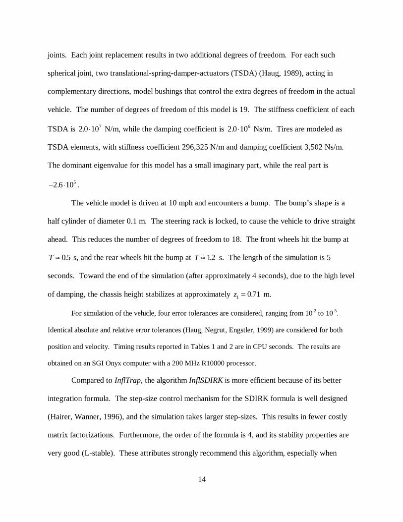
14
joints. Each joint replacement results in two additional degrees of freedom. For each such
spherical joint, two translational-spring-damper-actuators (TSDA) (Haug, 1989), acting in
complementary directions, model bushings that control the extra degrees of freedom in the actual
vehicle. The number of degrees of freedom of this model is 19. The stiffness coefficient of each
TSDA is 2 0 107. ◊ N/m, while the damping coefficient is 2 0 106. ◊ Ns/m. Tires are modeled as
TSDA elements, with stiffness coefficient 296,325 N/m and damping coefficient 3,502 Ns/m.
The dominant eigenvalue for this model has a small imaginary part, while the real part is
- ◊2 6 105. .
The vehicle model is driven at 10 mph and encounters a bump. The bump’s shape is a
half cylinder of diameter 0.1 m. The steering rack is locked, to cause the vehicle to drive straight
ahead. This reduces the number of degrees of freedom to 18. The front wheels hit the bump at
T ª05. s, and the rear wheels hit the bump at T ª12. s. The length of the simulation is 5
seconds. Toward the end of the simulation (after approximately 4 seconds), due to the high level
of damping, the chassis height stabilizes at approximately z1 0 71= . m.
For simulation of the vehicle, four error tolerances are considered, ranging from 10-2 to 10-5.
Identical absolute and relative error tolerances (Haug, Negrut, Engstler, 1999) are considered for both
position and velocity. Timing results reported in Tables 1 and 2 are in CPU seconds. The results are
obtained on an SGI Onyx computer with a 200 MHz R10000 processor.
Compared to InflTrap, the algorithm InflSDIRK is more efficient because of its better
integration formula. The step-size control mechanism for the SDIRK formula is well designed
(Hairer, Wanner, 1996), and the simulation takes larger step-sizes. This results in fewer costly
matrix factorizations. Furthermore, the order of the formula is 4, and its stability properties are
very good (L-stable). These attributes strongly recommend this algorithm, especially when

15
Table 1. Timing Results InflTrap Table 2. Timing results InflSDIRK
TOL 10-2 10-3 10-4 10-5 TOL 10-2 10-3 10-4 10-5
1 s 42 61 158 463 1 s 33 52 90 1702 s 79 155 420 1198 2 s 69 124 218 4333 s 92 189 524 1521 3 s 81 150 248 4934 s 100 206 552 1568 4 s 84 155 256 500
very stiff models are integrated with medium to high accuracy requirements. For low accuracy,
the difference between the algorithms is not significant.
In order to see the impact of the proposed algorithms on simulation timing results, they
are compared with a state-of-the-art explicit algorithm, in terms of efficiency. The explicit
algorithm used is denoted ExplDEABM. It is based on the code DEABM from the suite DEPAC
of explicit integrators of Shampine and Gordon (1975). ExplDEABM is an algorithm based on a
state-space reduction method, which uses the code DDEABM to integrate independent
accelerations to obtain independent velocities and positions. Dependent positions and velocities
are recovered using the position and velocity kinematic constraint equations of Eqs. (1) and (2).
Efficient means for acceleration computation are used in ExplDEABM, (Serban, Negrut, Potra,
Haug, 1997).
Table 3 presents simulation timing results in CPU seconds for ExplDEABM, which can
be compared with the results in Tables 1 and 2. The first row contains the absolute and relative
error tolerances imposed on both positions and velocities. The first column contains simulation
lengths in seconds. The simulations are carried out using the same SGI Onyx computer.
Table 3. Timing Results for ExplDEABM
TOL 10-2 10-3 10-4 10-5
1 s 3618 3641 3667 36632 s 7276 7348 7287 72763 s 10865 11122 10949 109654 s 14480 14771 14630 14592

16
The explicit algorithm requires up to 100 times longer to complete simulations,
independent of simulation duration and error tolerances. Results obtained with ExplDEABM also
conform to theoretical predictions; i.e., for each imposed error tolerance, the algorithm required
the same CPU time to complete a simulation run. This is typical of situations in which explicit
algorithms are limited to small step-sizes by stability considerations when integrating stiff
systems (Hairer, Wanner, 1996). Furthermore, for an imposed error tolerance, the CPU time
increases linearly with the simulation length. Even after the vehicle clears the obstacle and there
is no significant source of external excitation, the explicit algorithm is constrained to take very
small steps, because otherwise it would become unstable.
4. Topologically-Based Sparse Matrix Linear Equation Solvers
The equations of motion of Eq. (4) and kinematic acceleration equations of Eq. (3), for a
multibody system, may be written in matrix form as
M0
q Qq
q
FF
TLNMM
OQPPLNM
OQP = L
NMOQP
&&l t (26)
The coefficient matrix of the linear system in Eq. (26) is of dimension ( ) ( )n m n m+ × + , and is
called the augmented matrix.
The strategy proposed for solving the linear system in Eq. (26) proceeds by formally
expressing accelerations &&q in terms of Lagrange multipliers. Assuming for the moment that the
mass matrix is nonsingular, accelerations are substituted back into the acceleration kinematic
constraint equation to obtain
Φ Φ Φq q qM M Q− −= −1 1Td iλ τ (27)
17
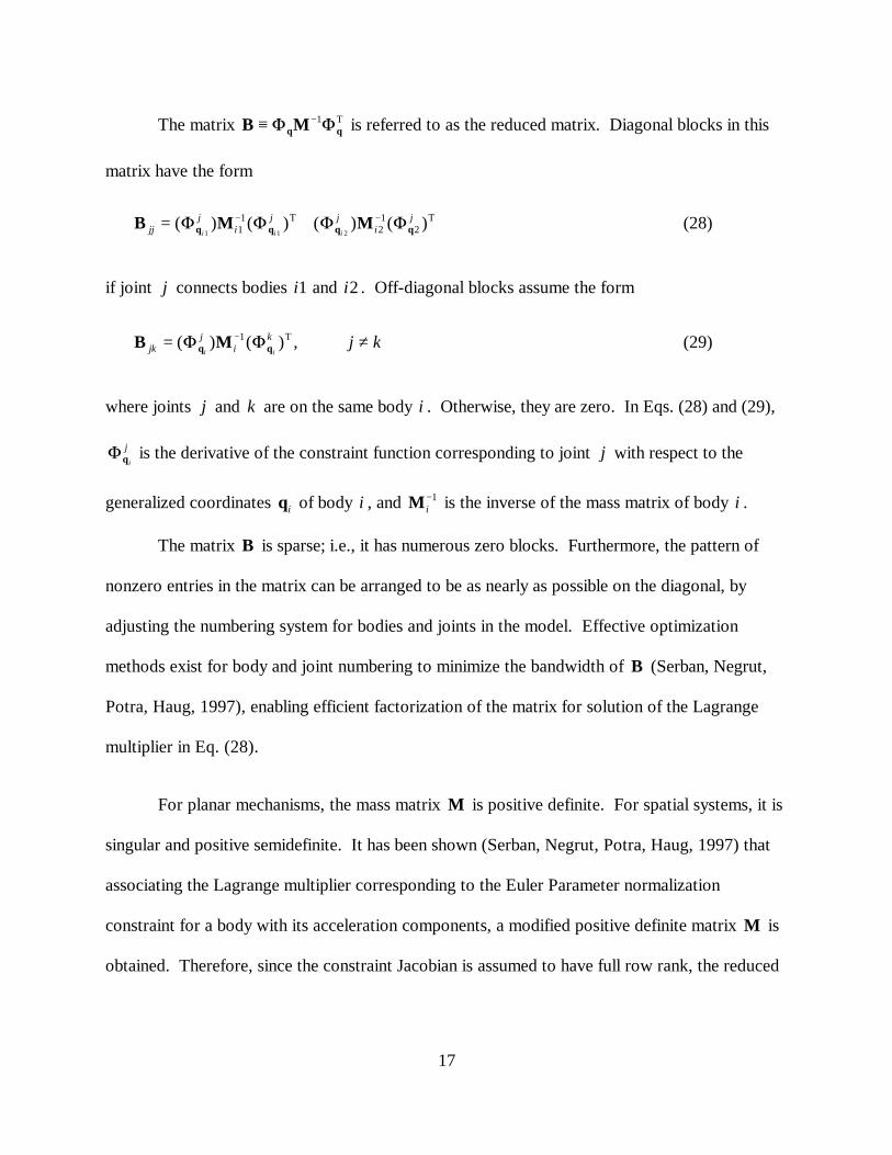
The matrix B Mq q≡ −F F1 T is referred to as the reduced matrix. Diagonal blocks in this
matrix have the form
B M Mq q q qjjj
ij j
ij
i i i= +− −( ) ( ) ( ) ( )F F F F
1 1 211
21
2T T (28)
if joint j connects bodies i1 and i2 . Off-diagonal blocks assume the form
B Mq qjkj
ik
i ij k= ≠−( ) ( ) ,F F1 T (29)
where joints j and k are on the same body i . Otherwise, they are zero. In Eqs. (28) and (29),
F qi
j is the derivative of the constraint function corresponding to joint j with respect to the
generalized coordinates qi of body i , and Mi− 1 is the inverse of the mass matrix of body i .
The matrix B is sparse; i.e., it has numerous zero blocks. Furthermore, the pattern of
nonzero entries in the matrix can be arranged to be as nearly as possible on the diagonal, by
adjusting the numbering system for bodies and joints in the model. Effective optimization
methods exist for body and joint numbering to minimize the bandwidth of B (Serban, Negrut,
Potra, Haug, 1997), enabling efficient factorization of the matrix for solution of the Lagrange
multiplier in Eq. (28).
For planar mechanisms, the mass matrix M is positive definite. For spatial systems, it is
singular and positive semidefinite. It has been shown (Serban, Negrut, Potra, Haug, 1997) that
associating the Lagrange multiplier corresponding to the Euler Parameter normalization
constraint for a body with its acceleration components, a modified positive definite matrix M is
obtained. Therefore, since the constraint Jacobian is assumed to have full row rank, the reduced

18
matrix B is positive definite. Since Lagrange multipliers are available from the solution of Eq.
(27), accelerations are easily computed using the equations of motion,
Mq Q q&&= − F Tl (30)
The mass matrix M has the block diagonal structure
M
M 0 00 M 0
0 0 M
=
L
N
MMMM
O
Q
PPPP
1
2
LK
L L L LL nb
(31)
For both planar and spatial systems, the block diagonal terms have closed form inverses
(Serban, Negrut, Potra, Haug, 1997), so M is easily inverted. The proposed algorithm for
solving Eq. (27) for Lagrange multipliers and accelerations is thus as follows:
(1) Assemble the reduced matrix B , based on Eqs. (28) and (29).
(2) Solve the linear system of Eq. (27) for l.
(3) Recover the generalized accelerations, based on Eqs. (30) and (31).
Steps 1 and 2 are discussed in detail by Serban, Negrut, Potra, and Haug (1997). They are
responsible for the better efficiency of the method, when compared to classical direct methods.
During these two steps, advantage is taken of the topology-induced sparsity. Step 3 requires the
solution of nb systems of linear equations of dimension 3 3¥ for planar systems and 7 7× for
spatial systems, to recover generalized accelerations. This process can be carried out in parallel.
At the core of the proposed algorithm for solution of the augmented linear system of Eq.
(26) is an efficient factorization of the reduced matrix B (Serban, Negrut, Potra, Haug, 1997).
The factorization takes advantage of the sparsity induced by the topological graph of the

19
mechanical system. The following four algorithns, based on combinations of solution sequences
and linear solvers, are compared:
(1) The Lapack dense linear solver dgetrf-dgetrs, based on LU decomposition for general
matrices, is applied to the augmented linear system of Eq. (26) to evaluate both accelerations and
Lagrange multipliers.
(2) The Harwell sparse solver ma47, based on LU decomposition of symmetric matrices, is used
to solve the augmented linear system of Eq. (26).
(3) The Harwell Cholesky decomposition routine ma35, for banded symmetric, positive definite
matrices, is used to factor the reduced matrix B and solve Eq. (27) for the Lagrange multipliers
corresponding to joint constraints. Accelerations and Lagrange multipliers for Euler parameter
constraints are then recovered using Eq. (30).
(4) The Lapack Cholesky decomposition routine (dpbtrf) for banded symmetric, positive definite
matrices, replaces the Harwell routine of algorithm 3.
Numerical results presented in Table 4 are based on the proposed algorithms and refer to
the HMMWV-14 model presented in Sections 2 and 3. For this example, the proposed solution
technique is compared with the usual direct approach of solving for the generalized accelerations
and Lagrange multipliers by factoring the augmented matrix. The most efficient solution
technique is the last. The speed-up obtained from the usual strategy for solving the augmented
system, using a sparse LU decomposition (algorithm 2), is a factor of 4.2. The small difference
between algorithms 3 and 4 is due to the different internal storage algorithms in the subroutines
dpbtrf from Lapack and ma35 from Harwell.

20
Table 4. Timing Results for HMMWV-14 Numerical Experiments
Algorithm 1 Algorithm 2 Algorithm 3 Algorithm 4
22.88 ms 12.62 ms 3.17 ms 3.07 ms
5. Analytical Differentiation Identities
As shown in Section 3, implicit integration of the equations of multibody dynamics
requires the availability of a derivative of the differential equations of motion and third order
derivatives of the algebraic constraint equations. Regardless of which implicit integrator is used,
derivatives of all terms in Eqs. (1) through (4) with respect to both generalized coordinates and
velocities are required. The derivatives to be evaluated are as follows:
As shown by Serban and Haug (1998a), in the setting of Cartesian coordinates with Euler
parameters for orientation, a relatively small number of basic identities enables computation of
all required derivatives. Explicit forms for derivatives of basic quantities are obtained.
Therefore, this approach is expected to be more efficient than using automatic differentiation
methods (Bischof, et.al., 1996). When evaluating higher order derivatives, automatic
differentiation codes differentiate a lower order derivative and thus cannot take advantage of
simplifying identities that may exist, such as Euler parameter normalization constraints.
In the proposed approach, derivatives of four basic expressions that are used as building
blocks in generating required kinematic and kinetic derivatives are obtained. The identities
derived are subsequently applied to obtain higher order derivatives of the four basic constraints
on vectors in and between pairs of bodies (DOT-1 constraint, DOT-2 constraint, distance
( &&) , ( ) , , ( &) , ( &&) , (( &) &) , (( &) &)& &Mq Q , Q q q q q q qq qT
q q q q q q q q q q q q qΦ Φ Φ Φ Φλ

21
constraint, and spherical constraint) (Haug, 1989), which are then combined to generate
derivatives of constraints corresponding to any kinematic joint. A similar treatment is applied to
obtain derivatives of common force elements.
Numerical experiments have shown significantly improved efficiency of computation
using the expressions derived, compared with results obtained employing finite differences. For
the 14-body model of the HMMWV, Table 5 presents maximum absolute differences between
analytical and numerical values of the kinematic derivatives, for different values of the
perturbation used in computing finite differences.
Table 5. Kinematic Derivative Comparison (Analytical vs. Finite Difference)
Perturbation 10-4 10-5 10-6 10-7 10-8
Φ q 3.291�10-3 3.291�10-4 3.291�10-5 3.293�10-6 3.241�10-7
Φ q q
Tλd i 4.012�10-2 4.012�10-3 4.013�10-4 4.002�10-5 5.864�10-6
Φ q qq&d i 5.301�10-2 5.599�10-3 5.599�10-4 5.655�10-5 1.148�10-5
Φ q q qq q& &d ie j 10.5970 1.0587 0.1059 1.054�10-2 2.254�10-3
Φ q q qq q& &
&d ie j 6.582�10-3 6.582�10-4 6.538�10-4 1.482�10-4 1.322�10-4
A library of subroutines that calculate the required derivatives outlined above has been
implemented in the computational environment described in Section 2. This library is used for
calculating derivatives required for implicit integration in Section 3, constructing the matrices
factored using the topological method of Section 4, and in implementing the globally
independent coordinate, real-time simulation method described in Section 7.
6. Dual-Rate Numerical Integration Methods
If a wide range of frequencies are present in the system to be simulated, different step-
sizes can be used within a multi-rate integration formula to speed up computations. Multi-rate

22
methods possess the potential for real-time vehicle simulation, due to the inherent structure of
the vehicle. Predominant frequencies in the motion of vehicles are in the range of 1 to 2 Hz for
the sprung mass (chassis) and 10 to 15 Hz for the un-sprung mass (suspension system), during
wheel hop (Gillespie, 1992). Much higher frequencies are observed for wheel spin and tire force
calculation (Bernard, 1973). High frequency content is also encountered when modeling vehicle
subsystems such as powertrain, steering, braking, and active suspension.
The equations of motion employed here for dual-rate integration of constrained
mechanical systems are
M q q q Q q,q xqb g b g b g&& &,+ =Φ λT
(32
Φ q 0b g= (33)
& ,&, ,x q q x= Γ tb g (34)
where Eq. (34) is a set of n x ODE that is used to model interacting vehicle subsystems such as controls
and tire forces that influence forces on the vehicle, often containing high frequency effects.
During the simulation of vehicle systems, problems arise when subsystems with high
frequency content require small step-size for a stable solution, making the simulation process
inefficient. If this small step-size is used for all the variables in the system, the overall
simulation performance will suffer. Within computer hardware constraints imposed by
microprocessor technology, it may not be possible to solve the governing equations of the
vehicle model in real time. As a result, multi-rate numerical integration techniques that may
overcome the limitations of existing computational engines are needed.
Solis (1996) reviewed ODE multi-rate integration methods. Among the methods
presented, the slowest first approach (Wells, 1982) was chosen to be applied to the vehicle
simulation problem. Although this method was designed for integrating ODE, its application

23
was made possible by reducing the DAE that describe the vehicle motion, to an ODE on a
manifold, expressed in terms of the constraint equations. This reduction can be carried out using
a number of DAE solvers available in the literature. For the present work, the generalized
coordinate partitioning method (Haug, 1989) is combined with the globally independent
coordinate method (Serban, Haug, 1998) to reduce the DAE to underlying ODE.
The slowest first approach consists of integrating the slow variables first, using
extrapolated values of the fast variables (if implicit formulas are used for the slow integration),
and then integrating the fast variables using interpolated values of the slow variables. Because
the slow and fast variables are coupled, extrapolation of the fast variables in the slowest first
approach is subject to numerical errors. This is not relevant if explicit integration formulas are
used to integrate the slow variables, but it becomes critical when implicit formulas are used.
In Fig. 4, the smooth line represents slow variable ( q qi i and &) response and the zig-zag
line represents a typical fast variable ( x i+rk ) response. The slow variables are integrated using a
step- size h , and the fast coordinates are integrated using a step-size r = h / m r , where m r is a
fixed integer ratio between the step-sizes for both scales. Here, qip+ 1 and &qi
p+ 1 are predicted
position and velocity values for the slow variables. Finally, qi sr+* represents the interpolated
value of the slow variable for use in integrating for the fast variables.
This technique was implemented (Solis, 1996) and applied to the HMMWV-14 model,
using the null space method (Liang, Lance, 1987), instead of the coordinate partitioning-globally
independent coordinate approach of Section 7 to reduce the DAE to ODE. Very similar results
were obtained with a ratio of 6 between slow and fast integration step lengths.

24
Figure 4. Dual-Rate Integration Schematic
qi+ rk*
xixi+ rk
xi+ 1
xi− rxi− 2r&qi- 3
&qi- 2
&qi- 1
&qi
&&qi
&qip+ 1
qip+ 1
q
qi- 2
qi- 1
qi
Next, advantages of using multi-rate methods are discussed in terms of function
evaluation and numerical costs. Assuming the existence of two clearly identifiable time scales,
the process of integrating the slow subsystem over one step of size h is referred to as a macro
step, and the process of integrating the fast variables with a step-size r = h / m r is referred to as a
micro step. A complete multi-rate step contains one macro step and m r micro steps.
As the coupling between slow and fast variables decreases, the error accumulation during
integration decreases. Wells (1982) shows that multi-rate methods based on the slowest first
approach are convergent under certain conditions. Bounds for the absolute stability of multi-rate
methods are also presented. These technical conditions are derived from the absolute stability of
linear multi-step integration formulas.
The numerical cost of completing a multi-rate step can be measured in terms of several
contributing costs. Let C s be the cost of evaluating the slow time scale derivatives, C f be the cost of
evaluating the fast time scale derivatives, C intrp be the cost of interpolating the slow variables to provide
values needed by the fast subsystems, and C integ be the cost of performing one integration step using an
order k explicit multistep formula. The cost of one multi-rate integration step C mr is thus

25
C m C n C C (m n n ) Cmr r f coup interp s r f s integ= × + × + + × + ×d i (35)
In Eq. (35), n f , n s , and n coup are, respectively, the number of fast variables, slow variables, and
interpolated slow variables for use in the fast subsystems. If a single-rate integration method is used, the
step-size is dictated by the fast variables. The cost of single-rate integration in the same time interval is
thus
C m C m C m (n n ) Csr r f r s r f s integ= × + × + × + × (36)
It is assumed that the integration cost C integ is approximately equal to the interpolation cost
C interp , and the number of slow variables n coup that are interpolated (or extrapolated) is equal to the total
number of slow variables n s . The first assumption is reasonable if a multistep integration formula and a
consistent interpolation formula are used. The second assumption tends to reduce the overall advantage
of multi-rate methods, since coupling between slow and fast subsystems is often through a few variables
and not the whole set of slow variables. With these assumptions, Eq. (35) becomes
C m C n C C (m n n ) Cm r f s integ s r f s integr= × + × + + × + ×d i (37
which can be rearranged and simplified as
C m C C m n n n Cmr r f s r f s s integ= × + + × + + ×d ie j (38)
The condition under which a multi-rate integration formula is advantageous is
m 1 C n C 0r s s integ− × − × >b g (39)
which, in terms of the step ratio m r , is
m 1n C
Crs integ
s
> +×
(40)
Equation (40) shows that when an explicit multistep integration formula (only one
function evaluation per step) is used in a multi-rate integration method, the multi-rate integration

26
has a computational advantage over single-rate methods if the function evaluation cost per
variable is higher than the interpolation cost per variable. In constrained mechanical systems,
this is generally the case. With the reduction in computational cost in the solution of the system
equations, a reduction in computational time is also obtained. This goal justifies the use of
multi-rate formulas.
7. Globally Independent Coordinates
Numerical methods for real-time multibody system simulation and analysis must resolve
two conflicting requirements; (1) high fidelity of the model for high accuracy of results, and (2)
high computational efficiency for low simulation time. In the past, a number of modeling
approaches have been used to achieve one or the other of these goals. Commercial analysis tools
such as DADS and ADAMS that emphasize high fidelity are based on Cartesian coordinates,
while more recent codes designed for real-time simulation employ joint relative coordinate
recursive formulations (Bae, Haug, 1987a,b).
It is desirable that the same model be used for both fast and high fidelity simulations.
The Cartesian coordinate formulation with Euler parameters for orientation (Haug, 1989) is well
suited for multibody system modeling, from the point of view of systematic analysis, because of
the simple structure of the resulting equations. The main disadvantage of this formulation is the
dimension of the problem to be solved. A large system of DAE must thus be solved, which is a
computationally demanding task. State-space methods for solving the equations of motion, such
as those presented in Section 3, are based on a parameterization of the constraint manifold via a
set of independent coordinates. The equations of motion can theoretically be reduced then to a
set of ODE in these independent coordinates. However, for general mechanisms, such a
parameterization of the constraint manifold is possible only locally. Therefore, the underlying

27
ODE can be constructed only locally. When the manifold parameterization is no longer valid,
new independent coordinates must be selected, based on matrix decomposition techniques that
are in general computationally expensive.
Coordinates that are independent for the entire range of admissible motion, called
globally independent coordinates (GIC), are particularly attractive for multibody system
simulation. The existence of such coordinates eliminates the need for local independent
coordinate selection to parameterize the constraint manifold. For the special case of vehicle
multibody systems, Serban and Haug (1998) have shown that information on functional intent
and design criteria enables definition of a subset of generalized coordinates that remain
independent for the entire admissible range of motion. These coordinates are dual to force
elements of the vehicle system, including suspension springs, shock absorbers, and control
elements such as the steering rack.
In addition to the immediate advantage of avoiding the computationally expensive
redefinition of local parameterization in a state-space formulation, efficiency enhancements are
obtained from the fact that optimal computational sequences for dependent coordinate recovery
can be defined using the GIC formulation. Once values of independent generalized coordinates
and velocities are obtained by integration, dependent states and velocities are recovered from the
nonlinear constraint equations, usually using a Newton-Raphson or Newton-like method
(Atkinson, 1989). The dimension of this nonlinear system of equations is large, especially when
Cartesian coordinates with Euler parameters for orientation are used. Availability of GIC
associated with force and/or control elements in the multibody system results in a decoupling of
the nonlinear constraint equations into smaller sets of independent equations. Since the number
of equations being solved has a significant influence on the computational effort in solving sets

28
of nonlinear equations, recovery of dependent coordinates can be performed efficiently by
solving lower dimensional subsets of equations. Even greater efficiency is realized when these
solutions are obtained in parallel on a multiprocessor computer.
As an example of dynamic simulation using GIC, a 10-body HMMWV model is
presented. This model is obtained from the 14-body model of Fig. 3 by replacing the upper
control arms with composite revolute-spherical joints. Globally independent coordinates are
selected as lengths of suspension springs, position of the steering rack, position coordinates of
the center of gravity of the chassis, and three independent Euler parameters. A realistic slip-
based tire model is employed, requiring use of the dual-rate integration method of Section 6 in
integration for wheel rotation. In the simulation, the vehicle is initially moving at a speed of 5
m/s, and is driven for 4 s over a series of bumps.
In order to highlight the improved computational efficiency of the GIC formulation, this
method is compared to the usual generalized coordinate partitioning technique (Haug, 1989).
The topology-based linear solver presented in Section 4 is used to compute generalized
accelerations. The following three cases are compared:
GIC; The globally independent coordinate method, using the topology based linear solver
GCP1; The generalized coordinate partitioning method, using the topology based linear solver
GCP2; The generalized coordinate partitioning method, using sparse linear solver ma47 from
the Harwell library for acceleration computation
The last case serves as a reference, since it is the method currently used in the commercial
multibody dynamics software system DADS. All three cases use a constant step-size third order
Adams-Bashforth (AB3) integrator. All computations are performed on an SGI computer with
200MHz R10000 processors.

29
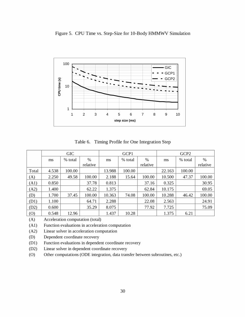
For integration step-sizes ranging from 10 ms to 1 ms, CPU times for a four second
simulation are plotted in Fig. 5. It can be seen that the computational effort for one integration
step with the GIC formulation is about 4.5 ms. This shows that real-time simulation can be
achieved with the GIC formulation, as long as the integration step-size is 4.5 ms or greater,
which is acceptable for this vehicle model. For the experiment considered, the generalized
coordinate partitioning algorithms use the same subset of independent coordinates throughout the
entire simulation. Therefore, the improved efficiency of the GIC formulation, as compared to
the GCP1 algorithm is due entirely to the dependent coordinate recovery algorithm. The speed-
up obtained for this portion of the numerical simulation is best seen in Table 6, which presents
the timing profile for one step of numerical integration for each of the three algorithms
considered. The proposed computational sequence for dependent coordinate recovery is faster
than the conventional method by a factor of 6.1. Overall, it is a factor of 4.9 times faster.
This example illustrates the feasibility of the GIC formulation in achieving real-time
simulation, with a relatively high fidelity vehicle handling model. The formulation holds great
potential for implementation on shared memory parallel processors, which will enable real-time
simulation of even higher fidelity design oriented models in a virtual proving ground
environment.
30
Figure 5. CPU Time vs. Step-Size for 10-Body HMMWV Simulation
Table 6. Timing Profile for One Integration Step
GIC GCP1 GCP2ms % total %
relativems % total %
relativems % total %
relativeTotal 4.538 100.00 13.988 100.00 22.163 100.00(A) 2.250 49.58 100.00 2.188 15.64 100.00 10.500 47.37 100.00(A1) 0.850 37.78 0.813 37.16 0.325 30.95(A2) 1.400 62.22 1.375 62.84 10.175 69.05(D) 1.700 37.45 100.00 10.363 74.08 100.00 10.288 46.42 100.00(D1) 1.100 64.71 2.288 22.08 2.563 24.91(D2) 0.600 35.29 8.075 77.92 7.725 75.09(O) 0.548 12.96 1.437 10.28 1.375 6.21(A)(A1)(A2)(D)(D1)(D2)(O)
Acceleration computation (total)Function evaluations in acceleration computationLinear solver in acceleration computationDependent coordinate recoveryFunction evaluations in dependent coordinate recoveryLinear solver in dependent coordinate recoveryOther computations (ODE integration, data transfer between subroutines, etc.)
1
10
100
1 2 3 4 5 6 7 8 9 10
step size (ms)
CPU
tim
e (s
)
GICGCP1GCP2

31
8. Conclusions and Future Work
The following high-speed numerical simulation capabilities have been developed and
demonstrated, for use in CAE and in real-time driver-in-the-loop simulation:
(1) High fidelity dynamic analysis of vehicle models with stiff components, using
recently developed implicit integration algorithms, yields speed-ups of at least two orders of
magnitude over commercially available tools.
A new class of implicit SDIRK methods, developed for solution of stiff ODE, has been
adapted for solution of the DAE of multibody dynamics. Both fast low-order and more refined
higher order methods have been demonstrated. The new class of Runge-Kutta-based implicit
integrators is shown to overcome limitations in stability of lower order Newmark-based
algorithms. The more refined algorithms are targeted for highly accurate simulation of very stiff
vehicle system models, which are often encountered in vehicle system engineering. Topology-
based linear algebra tools discussed in Section 4 provide a highly efficient framework for the
computationally intense Rosenbrock and SDIRK methods. The benefits of the new implicit
numerical integrators is demonstrated for simulation of a bushed HMMWV14-body model.
This capability is currently being extended and implemented in the commercial DADS
software system for vehicle system engineering, under a grant from the U.S. National Science
Foundation. The formulation, extended to incorporate discontinuous effects due to intermittent
motion and variable model structure, will be made available to the commercial sector by LMS-
CADSI in the near future.
(2) Real-time simulation of vehicle models of comparable fidelity to those used by
industry in vehicle design for handling has been demonstrated, using the globally independent
coordinate formulation, topological linear solvers, and dual-rate numerical integration algorithms.
32
In order to demonstrate the real-time capabilities of the GIC formulation, in conjunction
with topology-based linear solvers and dual-rate integrators, a 10-body model of the HMMWV is
implemented and simulated in real time on multiprocessor computers that are commonly used in
driving simulators. Simulations used to test and demonstrate the capability developed include
steering, tire, and powertrain models that are at a level of fidelity suitable for vehicle system design.
The real-time simulation environment developed is now being implemented jointly by the
research team and Army personnel for interactive simulation with Army motion-based
simulators, such as the Ride Motion Simulator shown in Fig. 6, and the National Advanced
Driving Simulator shown in Fig. 7. With this capability, these enormously capable, state-of-the-
art vehicle driving simulators will function as virtual proving grounds for engineering
development of both on-and off-road vehicles and equipment.
Figure 6. Ride Motion Simulator

33
Figure 7. National Advanced Driving Simulator
Acknowledgement: This research was supported by the US Army Tank-Automotive Research,
Development, and Engineering Center through the Automotive Research Center (DoD contract
number DAAE07-94-C-R094), a multi-university Center led by the University of Michigan.
References
Atkinson, K. E., 1989, An Introduction to Numerical Analysis, Wiley & Sons, New York.
Bae, D.-S., Haug, E. J., 1987a, “A Recursive Formulation for Constrained Mechanical System
Dynamics. Part I: Open-Loop Systems”, Mechanics of Structures and Machines, Vol. 15, pp.
359-382.
Bae, D.-S., Haug, E. J., 1987b, “A Recursive Formulation for Constrained Mechanical System
Dynamics. Part 11: Closed-Loop Systems”, Mechanics of Structures and Machines, Vol. 15, pp.
481-506.

34
Bernard, J. E., 1973, “Some Time-Saving Methods for the Digital Simulation of Highway
Vehicles,” Simulation, pp. 161-165.
Bischof, C., Roh, L., Mauer, A., 1996, “ADIC: A Tool for the Automatic Differentiation of C
Program”, Technical report, Mathematics and Computer Science Division, Argonne National
Laboratory.
Corwin, L. J., Szczarba, R. H., 1982, Multivariable Calculus, Marcel Dekker, New York.
Gillespie, T. D., 1992, Fundamentals of Vehicle Dynamics, Society of Automotive Engineers.
Hairer, E., Nørsett S. P., Wanner, G., 1993, Solving Ordinary Differential Equations I. Nonstiff
Problems, Springer-Verlag, Berlin.
Hairer, E., Wanner, G., 1996, Solving Ordinary Differential Equations II. Stiff and Differential-
Algebraic Problems, Springer-Verlag, Berlin.
Haug, E. J., 1989, Computer-Aided Kinematics and Dynamics of Mechanical Systems, Allyn
and Bacon, Boston.
Haug, E. J., Iancu, M., Negrut, D., 1997, “Implicit Integration of the Equations of Multibody
Dynamics in Descriptor Form,” Advances in Design Automation, 1997 ASME Design
Automation Conference.
Haug, E. J., Negrut, D., Engstler, C., 1999, “Implicit Runge-Kutta Integration of the Equations of
Multi-Body Dynamics in Descriptor Form,” Mechanics of Structures and Machines, to appear.
Gear, C. W., Wells, D. R., 1984, “Multirate Linear Multistep Methods,” BIT 24, pp. 484-502.
35
Liang, C. G., Lance, G. M., 1987, “A Differentiable Null Space Method for Constrained Dynamic
Analysis,” Journal of Mechanisms, Transmissions, and Automation in Design, Vol. 109, pp. 405-411.
Schiehlen, W., 1994, “Symbolic Computations in Multibody Systems”, Computer-Aided
Analysis of Rigid und Flexible Mechanical Systems, (M. F. O. S. Pereira and J. A. C. Ambrosio
eds.), Kluwer Academic Publishers, pp. 101-136.
Serban, R., Haug, E. J., 1988a, “Analytical Derivatives for Multibody System Analyses,”
Mechanics of Structures and Machines, Vol. 26, pp. 145-173.
Serban, R., Haug, E. J., 1998b, “Dual Coordinates for Real-Time Vehicles Simulation,” Journal
of Mechanical Design, submitted.
Serban, R., Negrut, D., Potra, F. A., Haug, E. J., 1997, “A Topology Based Approach for
Exploiting Sparsity in Multibody Dynamics in Cartesian Formulation,” Mechanics of Structures
and Machines, Vol. 25, pp 379-39.
Shampine, L. F., Gordon, M. K., 1975, Computer Solution of Ordinary Differential Equations.
The Initial Value Problem, Freeman and Company, San Francisco.
Solis, D., 1996, “DAE Multirate Methods for Dynamic Systems with Interacting Subsystems,”
Ph.D. Thesis, The University of Iowa.
Wehage, R. A., Belczynski, M., 1992, “High-resolution Vehicle Simulations Using Precomputed
Coefficients,” Transportation Systems, ASME, Vol. 44, pp. 311-325.

36
Wells, D. R., 1982, “Multirate Linear Multistep Methods for the Solution of Systems of Ordinary
Differential Equations,” Report UIUCDCS-R-82-1093 Department of Computer Science,
University of Illinois at Urbana-Champaign.