Numerical investigation of modeling frameworks and ...

This is the Accepted version of the article

Numerical investigation of modeling frameworks and geometric approximations on NREL 5 MW wind turbine

Citation: M. Salman Siddiqui, Adil Rasheed, Mandar Tabib, Trond Kvamsdal (2019). Numerical investigation of modeling frameworks and geometric approximations on NREL 5 MW wind turbine. Renewable Energy. 2019, vol. 132, 1058-1075. DOI:10.1016/j.renene.2018.07.062

This file was downloaded from SINTEFs Open Archive, the institutional repository at SINTEF http://brage.bibsys.no/sintef

M. Salman Siddiqui, Adil Rasheed, Mandar Tabib, Trond Kvamsdal

This is the Accepted version.It may contain differences form the journal's pdf version

;

RESEARCH ARTICLE

Numerical investigation of modeling frameworks andgeometric approximations on NREL 5MW wind turbineM. Salman Siddiqui1, Adil Rasheed2, Mandar Tabib2 and Trond Kvamsdal1

1Department of Mathematical Sciences, Norwegian University of Science and Technology, NO-7491 Trondheim, Norway.2CSE Group, Mathematics and Cybernetics, Sintef Digital, 7034, Trondheim, Norway.

ABSTRACT

The key to the better design of an industrial scale wind turbine is to understand the influence of blade geometry andits dynamics on the complicated flow-structures. An industrial-scale wind turbine can be numerically represented usingvarious approaches (from simpler 2D steady flow to complex 3D with moving mesh, with and without the inclusionof hubs) that can alter the results substantially. At the same time, to standardize and test methodologies, the referenceindustrial-scale NREL 5 MW wind turbine is gaining popularity. The wind energy community will learn through animproved understanding of the aerodynamics of this NREL 5 MW reference mega−watt size wind turbine by takinginto consideration the various levels of geometric approximations. Hence, in this work the NREL 5MW reference windturbine is used for both: (a) understanding the associated flow-complexities due to various geometric approximation, and(b) comparison and validation of the performance of different numerical approaches for flow-simulation. The variousgeometric approximations considered here are related to simulating the influence of the shape of turbines structure (blade,an inclusion of hub, tower) and motions of blades. It involves (a) influence of 2D, 2.5D and 3D turbine blade geometryto highlight the impact of section bluntness, (b) influence of steady frozen rotor and rotating rotor simulations and (c)influence of inclusion of hub through a full-scale geometry of the complete reference turbine. Furthermore, the key featuresof the flow dynamics of a rotor and full machine are identified and parametric studies are conducted to evaluate overallperformance prediction under variable Tip Speed Ratios (TSR = 6, 6.5, 7, 7.5, 8, 8.5, 9) and variable level of geometricand flow modeling approximations.

KEYWORDS

Wind energy·Multipe reference frame·Sliding mesh interface·NREL 5MW wind turbine·Finite volume method

CorrespondenceM. Salman Siddiqui, Department of Mathematical Sciences, Norwegian University of Science and Technology, NO-7491 Trondheim,Norway.Phone: +47-48628035

E-mail: [email protected]

1. INTRODUCTION

The complex flow around wind machines, notably inside the near wake region, is hindering the universal development ofmegawatt-size wind turbines. It is essential to resolve the dominant source components of the flow to study the impact ofvariable environmental conditions on the turbine performance. Large rotor sizes and unique design of blade aerodynamiccharacteristics are also posing significant challenges [1]. It is necessary to limit the degrees of freedom to an acceptablelevel to quickly draw realistic conclusions [2]. Depending on the design complexity of a wind turbine, analytical, numericalor experimental based design approach can be adopted. The Blade Element Momentum (BEM) technique for the analyticalsolution of the turbine provides reasonable estimations in a short time frame [3]. The disadvantage of BEM is associatedwith its inability to predict the distributions of pressure and velocity magnitudes over the turbine structure [4][5]. On theother hand, the experimental tests conducted inside wind tunnels are also able to represent the flow field using methodssuch as Particle Image Velocimetry (PIV), however, due to ever-increasing sizes of modern wind turbines, experimentaltests at a real scale become almost impossible. To conduct experiments with downscale geometries are also not feasibleas the wind tunnel based conclusions can never be directly scaled to the actual dimensions [6]. Lacking a physical model

1

M.S.S M. Siddiqui et al.

NACA64-618

CYLINDER

DU21

DU25

DU35

DU30

DU40

Figure 1. NREL5MW: CAD model of the turbine blade showing 2D airfoil cross sections used in the design of wind turbine rotor blade

Figure 2. NREL 5MW: Illustration of the computational mesh over the domain of full-machine. The planar cross-section shows thefiner mesh grading employed near turbine surface and inside the wake block to capture sharp gradients. The mesh is composed of

tetrahedral and hexahedral elements and having y+ of 30.

of the turbine geometry also prevents experimental tests at the initial design stage. Numerical investigations based onComputational Fluid Dynamics (CFD) are recently emerging as an attractive alternative to the analytical and empiricalapproaches [7]. It allows to conduct high fidelity simulations at real scales and provide ease of visualization of the flowvariables (p,u) over the regions of interest. Current progress in CFD is still in its infancy due to the requirement of highcomputational resources. However, continued advancements in the computing technology are helping such simulations todeliver faster results. They are believed to aid wind engineers to draw plausible conclusions based on visual evidence [8].To employ CFD in earlier designs, the researchers have used various geometrical approximations of the wind turbinestructure to lower the computational cost. Most of the initial work thus was only focused on the simulation of the flowdynamics around airfoil/blade sections. In the context of 2D simulations, Devinant et al. and Sicot et al. [9][10] workhave particular significance. They have demonstrated the flow and stall behavior around the airfoils and demonstrated thatsimple 2D simulations are not enough to develop realistic estimates of the aerodynamic loading. Tangler et al. [11] also

2

M. Siddiqui et al. M.S.S

Table I. NREL 5MW: Detail of airfoils used in the construction of CAD model taken from [22]

Airfoil Profile Thickness (t/c) Begin location (m) Chord (m) Twist angle(o)

Cylinder1 100% 2.00 3.542 0.000Cylinder2 100% 5.60 3.854 0.000DU40-A17 40.50% 11.75 4.557 13.308DU35-A17 35.09% 15.85 4.652 11.480DU30-A17 30.00% 24.05 4.249 9.011DU25-A17 25.00% 28.15 4.007 7.795DU21-A17 21.00% 36.35 3.502 5.361NACA64-A17 18.00% 44.55 3.010 3.125

performed similar numerical tests in both 2D/3D and consistently monitored the accuracy of his numerical simulationsagainst experimental data. He also pointed the discrepancies of simple 2D simulations and the need for full-scale 3Dtests for the accurate prediction of aerodynamic loading. The study of three-dimensional effects has started to becomepronounced as the turbine blade was constructed with multiple airfoil sections. Irregular relative velocity distribution andvariable thickness along the span have produced transverse flow effects, which were necessary to be integrated into theanalysis. Spentzos et al. [12] thus have performed full numerical estimations and demonstrated that the flow separationaround the blade could cause transverse flow under dynamic conditions. Numerical modeling of a full-scale HorizontalAxis Wind Turbines (HAWT) at variable wind speeds (5.0 m/s to 10.0 m/s) was performed by Yu et al. [13]. They haveillustrated the phenomenon of stall delay and flow separation in a 2D/3D spatial environment. They associated the unusualvibrations in the turbine during operation to the massive flow separation and three-dimensional spanwise flow over thesuction surface of the blade. Sørensen et al. [14][15][16][17] performed aerodynamic simulations on rotors of mega-wattsize turbines with Ellipse3D. They have determined that full rotor modeling is essential to obtain realistic estimates ofthe flow inside the plane of the rotor as well as in the wake. Bazilevs et al. [18][19][20][21] performed the analysis ona full machine including the cylindrical tower and the nacelle into the computational framework. They have manifestedthat a loss in the overall torque occurs while the blade passes in front of the turbine tower. Therefore simpler geometricalapproximations are deemed to modify the results and sometimes aid to draw implausible conclusions related to windturbine performance.

Higher associated costs related to full-scale modeling have also forced the researchers to adopt various numericalapproximations. Siddiqui et al. [23] and Bazilev et al. [18] have performed the rotor simulations by modeling only the120 sector of the domain to reduce the numerical complexity (by exploiting the periodicity of the flow). Sørensen etal. [14][15] and Zhong et al. [24] have addressed the problem by replacing the turbine blades from the numerical frameworkwith actuator line or actuator disc models. Although it has provided substantial speed ups which allow analyzing the large-scale behavior (wind farm analysis), however, such approximations are believed to draw implausible conclusions towardsthe aerodynamic loading of the blades. Jasak et al. [25] have attempted to reduce the numerical complexity by the additionof source terms (centripetal and centrifugal forces) into the governing systems of equations to account for the rotationaleffects. Until now, the only handful of studies have incorporated the turbines physical rotation under fully resolved settingto assess the dynamic loading. The essential details for megawatt size turbines thus lack a clear understanding of thediscrepancies arising from the assumptions mentioned above on a single turbine model.

In the present work, we aim to present the numerical and geometrical approximations approaches for a full-scalemegawatt wind turbine. The goal is to illustrate the extent of each approximation using CFD and exhibit its implication onthe overall power production. Reynolds Averaged Navier-Stokes (RANS) simulation technique has been applied to conductthe simulations under fully resolved setting on industrial NREL 5MW reference wind turbine [22][26]. We have quantifiedthe overall torque, wake distribution, and turbulent structures formation in a 2D, 2.5D, 3D (blade, rotor, and full machine)configurations at various operating conditions. The authors have already conducted such study for a small rooftop VerticalAxis Wind Turbines (VAWT) and have demonstrated successfully the implications on overall power production [2][8][27].

2. THEORY

2.1. CAD model and NREL turbine

The 5MW NREL turbine consists of three 63m long blades defined in terms of cross-sectional Delft University (DU) andNational Advisory Committee for Aeronautics (NACA) profiles (DU21, DU25, DU30, DU35, DU40, and NACA64) withdifferent twist angles at various locations away from the hub [26]. The twist angles along the blade from hub to tip are

3


(a) Case-I: 2D airfoils (b) Case-II: Stationary blade

(c) Case-III: Rotating rotor (d) Case-IV: Rotating rotor exploiting axial symmetry

(e) Case-V: Rotating turbine with support structure and ground

Figure 3. NREL 5MW: Illustration of case setups employed with increasing level of geometric approximation. Note∗: R represents theradius of the turbine(61.9m)

4


0 5 10 15α

0.0

0.2

0.4

0.6

0.8

1.0

1.2

1.4

1.6

1.8

Cl

ExpNum

(a) NACA64

0 5 10 15α

0.4

0.6

0.8

1.0

1.2

1.4

1.6

Cl

ExpNum

(b) DU21

0 5 10 15α

0.0

0.5

1.0

1.5

Cl

ExpNum

(c) DU35

0 5 10 15α

0.0

0.5

1.0

1.5

Cl

ExpNum

(d) DU40

Figure 4. NREL 5MW: Comparison of Cl with experiments at four different sections of turbine blade. Error bars in blue color representsthe uncertainty associated with the experimental measurements

intended to accommodate the variations in the incoming relative wind velocity arising from the rotational motion of theblade. To prevent structural failure, a significant sectional thickness is required at the blade root close to the hub [28]. Itcalls for airfoils with a relatively higher thickness, typically 30% to 40% chord length near the hub [29]. Away from thehub, cross sections are more aerodynamically shaped to maximize lift and minimize drag to allow an increase in torquegeneration. A parametric Computer-Aided Design (CAD) model of the blade is generated using the data provided in TableI. The hub height is fixed at an elevation of 90m above the ground. The tower’s base diameter is 6m tapering with heightto 3.87m close to the hub.

2.2. Governing equations and numerical techniques

Flow around complex geometries is governed by the conservation equations of mass and momentum. However, therotational motion of wind turbines adds further complexity making the computations more expensive and prone to round-off errors (due to the presence of very high velocity close to the tip of the blade). To deal with such problems threedifferent techniques are adopted: Single Reference Frame (SRF), Multiple Reference Frame (MRF) and Sliding MeshInterface (SMI) [30]. While in the SMI technique, turbine rotation is explicitly resolved using a rotating mesh and unsteadysimulations, in the other two (SRF and MRF) the mesh is maintained stationary and appropriate source / sink terms areadded to the governing equations to model the steady-state behavior of the flow implicitly. A detailed technical descriptionof the three techniques is presented in the following subsection.

5


2.2.1. Single reference frameThis procedure is applied when there is only one center of rotation, and all the wall surfaces are rotating with the same

rotational speed. The general idea is to describe the flow from a reference frame attached to the rotating body and rewritethe governing equations in the rotating reference frame. It results in two additional terms in the momentum equationcorresponding to Centripetal and Coriolis forces (See second and third term on the left-hand side of Equation 2).

∇ · ur = 0 (1)

∂ua∂t

+∇ · (ur ⊗ ur) + 2Ω× ur︸︷︷︸Centripetal force

+ Ω× (Ω× r)︸︷︷︸Coriolis force

= −∇p+∇ · (ν + νt)∇(ur + (∇ur)T(2)

Where Ω is the rotational speed of the reference frame for a stationary observer (here it will also be equal to the rotationalspeed of the turbine), p is the pressure, ν is the kinematic viscosity of the air and νt is the turbulent kinetic viscosity. Sincesteady state solutions are aimed for, temporal derivatives are dropped from the governing equations both in SRF and MRF.

2.2.2. Multiple reference frameThe shortfall of SRF technique is that it requires all the solid walls/structures to be rotating around the same axis and

with the same rotational speed. It has limited applications in the current context where the rotor turbine rotates, however,the ground surfaces and the support structures are stationary. MRF technique eliminates those shortfalls by subdividing thecomputational domain into different non-overlapping zones each rotating with a different rotational speed. While in thefixed zones, the governing equations are addressed in the absolute reference frame, the equations describing flow in therotating zones are rewritten in the form similar to those of the SRF. At the interfaces boundaries between different zones, atransformation is applied to enable flow variables located inside one zone to be used to estimate fluxes at the boundary ofthe adjacent zone [25]. Velocities and velocity gradients are transformed from the rotating reference frame to the absoluteinertial frame using Equation 7. No such special treatment is applied to scalar quantities such as pressure, density, turbulentkinetic energy, and dissipation.

Thus in the stationary zone, following set of equations for mass and momentum are solved:

∇ · ua = 0 (3)

∂ua∂t

+∇ · (ua ⊗ ua) = −∇p+∇ · (ν + νt)∇(ua + (∇ua)T) (4)

where ua is the absolute velocity as seen from a SRF. In the rotating rotational zone, the same equations are rewritten interms of the relative speed ur (relative to the rotating frame of reference) given by:

∇ · ur = 0 (5)

∂ur∂t

+∇ · (ur ⊗ ur) + 2Ω× ur + Ω× (Ω× r) = −∇p+∇ · (ν + νt)∇(ur + (∇ur)T) (6)

ua = ur + Ω× r (7)

2.2.3. Sliding mesh interfaceBoth SRF and MRF seek steady-state solutions to problems that are inherently unsteady. To capture the transient

behavior, an accurate but computationally expensive [31] SMI technique is employed. In this, flow around a rotatingturbine at any particular instance is computed, after which, the mesh is rotated by an angle equal to the rotational speedof the turbine times a time step. The previously calculated flow field is then projected onto the revolved mesh and solvedfor the new time step. This technique thus explicitly captures the effects of rotation. The associated improvements are anaccurate balance of fluxes at the interface boundaries [32] and modeling of transient effects like pressure waves arising dueto the relative motion between the rotational and stationary zones. The governing equations remain in its original form.However, there is an additional step of mesh motion and projection of the computed field on the moving mesh at everytime step.

∇ · ua = 0 (8)

∂ua∂t

+∇ · (ua ⊗ ua) = −∇p+∇ · (ν + νt)∇(ua + (∇ua)T) (9)

6


0 5 10 15α

0.00

0.05

0.10

0.15

0.20Cd

ExpNum

(a) NACA64

0 5 10 15α

0.00

0.05

0.10

0.15

0.20

Cd

ExpNum

(b) DU21

0 5 10 15α

0.00

0.05

0.10

0.15

0.20

Cd

ExpNum

(c) DU35

0 5 10 15α

0.00

0.05

0.10

0.15

0.20

0.25

0.30

Cd

ExpNum

(d) DU40

Figure 5. NREL 5MW: Comparison of Cd with experiments at four different sections of turbine blade. Error bars in blue colorrepresents the uncertainty associated with the experimental measurements

2.3. Turbulence modeling

Flows encountered in wind turbine are highly turbulent and characterized by eddies having large spatio-temporal variations.These scales can be fully resolved using Direct Numerical Simulations (DNS) or partially using Large Eddy Simulation(LES). However, their high computational nature prohibits their usage for the kind of study undertaken in this work.We, therefore, used k − ε, k − ω and Spalart Allmaras (SA) models which are based on the RANS equations. A detaileddescription of SA turbulence model can be found in [33]. The two equation models k-ε and k−ω are given by the followingset of t, k, ε and ω equations [34][35]

∂k

∂t+∇ · (u⊗ k) = τij∇u +∇ ·

[ν + νtσk

]∇(k + (∇k)T)− ωk (10)

∂ε

∂t+∇ · (u⊗ ε) = Cε1

ε

kτij∇u +∇ ·

[ν + νtσε

]∇(ε+ (∇ε)T)− Cε2

ε2

k(11)

∂ω

∂t+∇ · (u⊗ ω) =

γ

νtτij∇u +∇ ·

[ν + νtσω

]∇(ω + (∇ω)T)− ω2β + 2(1− F1)

σω2ω∇.k∇.ω (12)

The model constants used in the study are σk1=0.85 σω1=0.65 β1=0.075 σk2=1.00 σω2=0.856 β2=0.0828β∗=0.09 a1=0.31

7


3. COMPUTATIONAL SETUP

3.1. Investigated cases, mesh and boundary conditions

Table II. NREL 5MW: Overview of the test cases investigated under various geometric and numerical assumptions

Sr. no Dimension Blade design Rotor Geometry Numerical Technique Mesh SizeCase-I 2D NACA64, DU21/35/40 - Airfoil SRF 0.3×106

Case-II 2D/2.5D/3D NREL 5MW 120 Blade SRF 2×106

Case-III 3D NREL 5MW 360 Rotor MRF/SMI 6×106

Case-IV 3D NREL 5MW 120 Blade MRF 2×106

Case-V 3D NREL 5MW 360 Rotor & monopole MRF/SMI 10×106

To study the influence of progressing complexities resulting from simulation set-up and simulation techniques, the studyis partitioned into five cases (see Table II). A brief classification of each case, its purpose and set-up are provided below.

Case-I 2D simulations of flow around blade sections (NACA64, DU21, DU35, DU40 airfoils): The objective of thesesimulations is two-fold; firstly to validate the model against experimental results. Secondly to get a quantitative idea of thevariation of lift and drag coefficient as a function of the angle of attack at a high Reynolds number. The choice of domainand boundary conditions are manifested in Figure 3(a). 3× 105 mesh elements are utilized in the simulation. The domainand mesh independence studies are previously exhibited in work by Nordanger et al. [36][37]. The resolutions used hereis twice the finest resolution employed in those studies.

Case-II 2D, 2.5D and 3D simulations of stationary turbine blade: The purpose of these simulations is to evaluate theapplicability of the use of lower spatial dimensions to model the flow physics. The 2D simulations are similar to the onesmentioned in Case I. The 2.5D simulations are conducted on slices around the four profiles (NACA64, DU21, DU35,DU40) of the blade. A similar investigation is performed by Sørensen et al. [38] and illustrated that RANS techniqueis capable of accurately predicting the spanwise structure. Herraez et al. [39] also suggested the similar conclusion,however, their study was limited to the smaller wind turbine at the root section only. The 3D simulation region is shown inFigure 3(b).

Case-III SMI and MRF simulation methods for flows around a rotating rotor: The goal of these simulations is to quantifythe discrepancies between accuracy and efficiency of the two methods to simulate rotational effects. The domain is shownin Figure 3(d). Six million mesh elements are applied to discretize the flow domain which is finer than the resolution usedby Bazilevs et al. [40] to simulate the fluid-structure interaction of the same turbine.

Case-IV Steady state simulation of flow around a single 3D rotating blade using MRF technique and utilizing axialsymmetry: The purpose of this study is to conduct several sensitivity studies (by changing turbulence intensity and TSR)at a reduced computational cost. Axial symmetry is utilized enabling the use of only one-third the domain used in CaseIII. The Periodic boundary condition is imposed on the lateral faces. The domain extent is chosen as defined by Bazilevset al. [40] in their study. The set-up is shown in Figure 3(c)

Case-V Simulation of the rotor with the nacelle, tower and ground effects using SMI and MRF: The purpose of this studyis to obtain a better insight into the consequences of a nacelle, tower, and ground on the wakes generated by the rotor. Thecase set-up is generated as suggested by Jonkman et al. [22] for full machine model of NREL 5MW. The estimation ofaerodynamic loading using CFD for complete 3D megawatt-size wind machine is proposed by Sørensen et al. [41][42].

A hybrid finite element mesh with structured hexahedral elements is created close to the structure, and the tetrahedralmesh is generated in the rest of the domain (see Figure 2). This approach not only permitted to produce a quality meshin the boundary layer adjacent to the turbine but also allowed more control over the y+ (standard wall functions are usedwith average y+ value of approximately 30). This way a hybrid mesh ensured a smooth transition from structured tounstructured mesh elements. The details of the computational setup and mesh sizes for all the cases are summarized inthe Table II. For the cases, III-V stationary and rotating sub-domains are separated by a non-overlapping interface. Therelative tolerance between the zone face is set low (approximately 0.0001) to make a tight interface coupling between theboundaries [25].

The simulations are conducted at various TSR’s for uniform and log-shaped velocity profiles for the case I-IV and caseV respectively. The TSR is adjusted by regulating the rotational speed (Ω) of the turbine. At the outlet face, standardoutflow boundary condition (zero gradients), is imposed for all the parameters computed. A free-slip boundary conditionis applied to the domain outer boundaries. To impose axial symmetry, the periodic boundary condition is employed on the

8


(a) d = 15m (b) d = 30m (c) d = 60m

Figure 6. NREL 5MW: Comparison of flow-pattern (velocity contour with superimposed streamlines) for 3D Vs 2.5D Vs 2D simulationat NACA64 section located 44.5m from the hub.

(a) d = 15m (b) d = 30m (c) d = 60m

Figure 7. NREL 5MW: Comparison of flow-pattern (velocity contour with superimposed streamlines) for 3D Vs 2.5D Vs 2D simulationat DU21 section located 36.5m from the hub.

(a) d = 15m (b) d = 30m (c) d = 60m

Figure 8. NREL 5MW: Comparison of flow-pattern (velocity contour with superimposed streamlines) for 3D Vs 2.5D Vs 2D simulationat DU35 section located 15.5m from the hub.

adjacent faces for the cases involving only the 120 model of the turbine. A no-slip boundary condition is applied on theblade surface, and wall function is used along with the k − ε and k − ω equations to work with relatively coarse meshclose to the blade surface [43].

9


(a) d = 15m (b) d = 30m (c) d = 60m

Figure 9. NREL 5MW: Comparison of flow-pattern (velocity contour with streamlines) for 3D Vs 2.5D Vs 2D simulation at DU40section located 11.75m from the hub.

3.2. Solver details

OpenFOAM-4.1 (OF), an open source CFD toolbox, is employed for the case studies enlisted in Table II. To ensure thatcontinuity is satisfied, the OF combines the continuity equation with the divergence of momentum equation to createan elliptic equation for the modified pressure. This elliptic equation along with the momentum and turbulence equationis solved in a segregated manner using either the PIMPLE algorithm (in transient case) or the Semi-Implicit Methodfor Pressure-Linked Equations (SIMPLE) algorithm (in steady state case). The OF uses a finite volume discretizationtechnique; wherein all the equations are integrated over control volumes (CV) using Green-Gauss divergence theorem.The Gauss divergence theorem converts the volume integral of the divergence of a variable into a surface integral of thevariable over faces comprising the CV. Thus, the divergence term defining the convection terms can simply be computedusing the face values of variables in the CV. The face values of variables are obtained from their neighboring cell centeredvalues by using convective scheme [37]. In this work, all the equations (except k and turbulence equations) use secondorder linear discretization scheme, while the turbulent equations use upwind convection schemes. Similarly, the diffusionterm involving Laplacian operator (the divergence of the gradient) is simplified to computing the gradient of the variable atthe faces. The gradient term can be split into the contribution from the orthogonal and non-orthogonal part, both of whichare considered in the analysis.

3.3. Other input parameters

For all the simulations, reference fluid density ρ = 1.225 kg/m3, dynamic viscosity µ = 1.82× 10−5 kg/m.s andincoming wind velocity U∞ = 9 m/s and turbine rotational speed Ω = 10 rpm is used. Several more simulations areconducted with the same inlet velocity but with seven different tip speed ratios (6, 6.5, 7, 7.5, 8, 8.5, 9). A self-adjustingtime step based on a maximum Courant number consideration of 1 is utilized. The simulations are terminated after 15000iterations for SRF/MRF and at least until 12 seconds corresponding to two turbine rotation for SMI simulations. It isensured that the residuals fall below 10−5 for all the simulations. The residual is calculated using the matrix systemAx = b as explained by Jasak et al. [44] in the following manner.

r =1

n

∑|b− Ax| (13)

where n is evaluated with residual scaling and using the normalization i.e. n =∑

(|Ax− Ax|+ |b− Ax|)

4. RESULTS AND DISCUSSION

In this section results from the simulations of the five cases are manifested in the increasing level of complexities. First,the results are exhibited in the form of validation and verification study performed in 2D. It is followed by a detailedcomparison of 2D/2.5D/3D simulation strategy. Herein, the simulations are presented for 120 and 360 sectors of theturbine rotor. In the end, the results are shown for a complete turbine consisting of nacelle and turbine tower.

10


Table III. NREL 5MW: Details of airfoil characteristics for 2D, 2.5D, 3D geometric approximations

Airfoil Distance from center (m) α () Chord (m)DU-21 36.35 -5.360 3.50DU-35 15.85 -11.48 4.65DU-40 11.75 -13.30 4.55NACA-64 44.55 +3.120 3.01

4.1. Case-I: 2D simulations of flow around blade sections

We have selected four airfoil sections (NACA64, DU35, DU21, DU40) from the NREL 5MW turbine blade to benchmarkthe numerical framework. The simulation is conducted under static conditions at the Re= 106 and multiple incidenceangles. Figure 4-5 illustrates a comparison of the aerodynamic coefficients prediction from present numerical setup againstthe experimental data. In general, a close agreement demonstrates the right design strategy and the suitable choice ofboundary conditions over the domain. Reliable estimates of the aerodynamic coefficients are essential since the torquecontribution is directly related to the amount of lift produced from the sections in the spanwise directions. The trend of liftcoefficient is such that it first rise with increasing α, reach a maximum value and then starts to drop again. It manifests theaccurate estimates of stall around the airfoil and shows the accuracy of numerical setup. Whereas, for the drag coefficientshigher magnitudes are seen for inner sections of the blade (constitutes of airfoils having higher thickness) as comparedto the outer sections (consist of more aerodynamically shaped airfoils). Slightly better agreements of coefficients at lowerα is associated with the extended symmetry of the flow about the chord length. The increase in α causes the flow tobecome unsymmetrical which leads to an inadequate agreement between the results. A notable rise in periodic oscillationsis reported after the critical α, which describes massive flow separation leading to the evolution of von-Karman vortexstreet in the wake behind the airfoils. For NACA64, DU21, DU35, the critical value of α is located in the proximity of 14.Whereas for DU40, it is found around 17. These measurements are in good agreement with the conclusions of Jonkmanet al. [22] who have conducted a similar experimental and analytical investigations on the airfoils.

4.2. Case-II: 2D, 2.5D and 3D simulations of stationary turbine blade

4.2.1. Wake distribution and flow structuresWind-turbine blades are designed for rotating conditions, where a realistic turbine blade thickness aims to taper from

root to tip enabling the blade to withstand higher stress and moment near the root than that towards the tip. Similarly,the blade twist is varied to maintain an optimum power coefficient (Cp) and α along the blade span. Now, the geometricoptimization works efficiently in operational conditions when the turbine is rotating. However, in a non-rotating situation,which can happen when yaw and pitch regulations are offline or during a turbine-erection phase, the blade twist optimizedfor rotation will cause the flow to become artificially 3D compared to the actual rotor flow itself. Hence, in the absenceof a wind turbine control situation during off-line, the α of flow on the blades is determined by the free wind direction,and the wind-turbine may operate outside the narrow operational range. In such stationary situations, complex 3D effectsmay exist owing to both the operating conditions and the 3D complex turbine geometry. Consequently, 2D simulationsconducted in the section 4.1 are not good enough to understand flow dynamics in such conditions. It now highlights thesignificance of performing stationary simulations which can account for the impact of bluffness of the turbine geometryand changing cross-section on aerodynamics parameters and flow physics. Therefore, this section provides results withthe stepwise increasing level of geometric approximation from 2D to 3D. 2D corresponds to the same setup as describedin the previous section, whereas, 3D simulation involves the full stationary NREL 5MW turbine blade. To get a deeperintuition of the flow behavior between the planar two and the full-scale three-dimensional simulations, a 2.5D dimension isintroduced. 2.5D segments are modeled by clipping the particular airfoil section from the full-scale 3D model and includethe tapering effects along the radial direction. Initially, the flow is simulated independently at all four segments (NACA64,DU35, DU21, DU40) before performing a static full-scale 3D blade simulations. This procedure highlights the changescaused in the flow field by the bluntness of a particular airfoil section, details of which are not captured by performingsimple 2D simulations. These intermediate spatial computations will account for three-dimensional effects with spanwisevariations of twist and the chord-length / blade thickness ratio. Here, a detailed comparison is presented regarding flowphysics and aerodynamic coefficients prediction by the three modeling approaches. The comparison provided in section4.1 for lift and drag coefficient with DOWEC report [45] is not applicable here anymore since the measured data is validfor the only 2D, where our 2.5D and 3D simulations take into consideration the tapering effects along the span as well. Acomparison of the simulations between the three approaches is manifested in Figure 6-9, which show the flow patterns atfour sections as predicted by 2D, 2.5D and 3D approach. Each airfoil section is set up at certain α, details of which aredescribed in Table III (which remained consistent for the three spatial dimensions). To identify the aerodynamic loading

11


0 10 20 30 40 50Distance from hub center radial direction (m)

0.02

0.00

0.02

0.04

0.06

0.08

0.10

0.12

0.14

Cd

DU40

DU35

DU21 NACA64

3D2.5D2D

0 10 20 30 40 50Distance from hub center radial direction (m)

0.8

0.6

0.4

0.2

0.0

0.2

0.4

Cl

DU40

DU35DU21

NACA64

3D2.5D2D

Figure 10. NREL 5MW: Comparison of computed aerodynamic drag and lift coefficients using 2D, 2.5D, 3D simulations at foursections of the blade.

from the three approaches quantitatively, drag and lift coefficients predictions from the simulation are plotted in Figure 10.Each section has reported a certain amount of separation along with vortex shedding of variable sizes and strengths at2D, 2.5D and 3D configurations. An examination of the contours highlights marked differences in the position of flowreversal point along the chord length in a particular setting. It is noted that the extent of flow reversal point varies from onegeometric approximation to another. The details of flow physics corresponding to each airfoil section is presented below:

NACA-64 airfoil: The outer part of the blade offers a significant contribution to the total torque production andexperiences relatively smaller loading. To fulfill both the requirements (maximum torque and minimum loading) NACA-64airfoils are employed in the outer part of the blade starting at a distance of 44.5m from the hub (Table III). The aerodynamicshape ensures that the flow is constantly attached to the blade surface. Figure 6 associates the flow patterns of velocitysuperimposed with flow streamlines for 2D, 2.5D, 3D. It is evident from the plots that there is negligible difference betweenthe three simulations of variable spatial dimensions, implying a lack of three-dimensionality and associated unsteadinessin the flow behavior. It can be attributed to the aerodynamic shape of the NACA64 profile and low α. Hence, the threesimulations converge to almost a single value of drag (Cd = 0.01) and lift (Cl = 0.1) coefficient(see Figures 10). Theabsence of oscillation in the computed values of coefficients also reinforces the absence of flow separation and associatedvortex shedding.

DU-21 airfoil: It is located at a distance of 36.5m from the hub center at an α = 5.3 (Table III). Comparable to thebehavior shown by NACA64 section, the flow is streamlined and strongly attached to the blade section(see Figure 7).No significant difference is observed between the three simulations, and the predicted values of drag and lift coefficientsare 0.01 and 0.2 respectively (Figure 10). The slightly higher value of the lift coefficient compared to one reported byNACA64 section can be attributed to slightly higher α. As the outer section of the blade is designed to produce maximumtorque, lesser separation is desirable which is also observed from the simulations. Moreover, being operated under higherrelative wind speeds most of the time increase the aerodynamic efficiency. Both sections(NACA64, DU21) offer large stallangles and are less likely to undergo a dramatic reduction in lift.

DU-35 airfoil: It is located at a distance of 15.5m from the hub center at an α = 11.48. Velocity contours withstreamlined for all three spatial simulations are shown in Figure 8. The streamlines in 3D configuration exhibit furthercomplex three-dimensional flow pattern beneath the airfoil surface. 2D and 2.5D results also show flow separations,whereas 2D show lesser chaotic streamlines than the 2.5D and 3D. In the downstream flow direction, snapshots of flowfield show a wavy velocity profile for 2.5D and 2D, where the streamlines arising from the top and bottom surfaces of theairfoil do not cross each other or mingle. On the other hand in the 3D simulations, the fluctuating profile is not observed.However, streamlines emanating from the bottom and top of the airfoil cross each other behind the airfoil implying threedimensionalities in the flow. This intermingling of the streamlines in 3D flow gets blended with expected higher turbulencewhich possibly diffuses the velocity profile. This flow separation and three-dimensional nature of the flow cause significantvariations in the predicted drag force. 2D and 2.5D predict a drag coefficient of nearly 0.11 whereas the 3D predict a dragof around 0.09 (see Figure 10(a)). In comparison to the NACA64 and DU21 segments, the 2D and 2.5D simulations for theDU35 section predict higher drag coefficients (Figure 10(a)). Comparison of the lift coefficient (Figure 10(b)), again hasshown a wide variation in the predicted values with all the three approaches. The 2D simulation altogether fails to predictthe trend, i.e., a decrease of lift coefficient while moving from turbine tip towards the hub.

12


0

500

1000

1500

2000

2500

3000

3500

k−

Om

eg

a−

SS

T(M

RF

)

k−

Om

eg

a−

SS

T(S

MI)

LE

S−

Sm

ag

orin

sky(S

MI)

k−

Ep

silo

n(M

RF

)

k−

Om

eg

a−

SS

T(M

RF

)

S−

A(M

RF

)

k−

Om

eg

a−

SS

T(M

RF

)

k−

Om

eg

a−

SS

T(S

MI)

Ba

zile

v−

et−

al.

Jo

nkm

an

−e

t−a

l. .

Aero

dynam

ic torq

ue(k

N m

)

Case−IIICase−IVCase−V

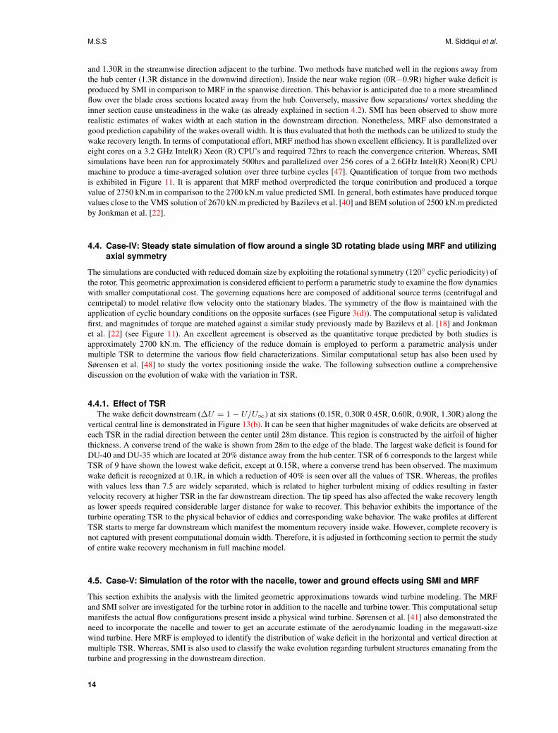
Figure 11. NREL 5MW: Comparison of aerodynamic torque using different simulation methodologies at TSR=7.5 compared againstBazilevs et al. [18] and Jonkman et al. [22]

DU-40 airfoil: It is the section located closest to the hub and is chosen for study at z = 11.75m with α = 13.3,which is placed at the highest α amongst the four sections. Here, the reported drag and lift coefficients values are higher inmagnitude than the ones for DU35, DU21, and NACA64. Similar to DU35, the DU40 case has also shown strong variationsin the predicted drag and lift coefficients from the three approaches (Figure 10). The 2D prediction has the largest dragand lowest lift coefficient for DU40 (amongst 3D and 2.5D) and have shown maximum deviation from the simulated 2.5Dand 3D drag and lift coefficient values. It could be due to the 2D nature of the predictions, which have a larger wake(which suggests higher form-drag acting in streamwise direction) as compared to 2.5D and 3D case. However, the lowerlift reported can be because of a balancing pressure distribution profile around the airfoil, since the streamlines emergingfrom airfoils bottom do not bend upwards as in the case of 3D and 2.5D (indicating a low reactive downward lift on theairfoil for the 2D case). The difference in the wake and streamlines behavior between 2D, 2.5D, 3D is shown in Figure 9.

Overall the results indicate that even for a stationary blade, the blade segments which are positioned nearer the to thehub are associated with complex 3D flow structures. These conclusions are also suggested by Herraez et al. [39] and Akayet al. [46] who performed PIV and CFD investigations on a horizontal axis wind turbine. Whereas, moving towards thetip of the blade, the associated flow tends to lose its 3D characteristics and can be represented by 2D simulations. As theouter part of the blade offers a notable contribution to the total torque generated, a 2D approach might be adequate topredict torque and hence power production from a turbine. It can be regarded as a justification for using an actuator linemodel to estimate power production from wind turbines. However, a 3D approach will still be required to predict unevenaerodynamic loading closer to the hub.

4.3. Case-III: SMI and MRF simulation techniques for flows around a rotating rotor

This section exhibits a comparison of SMI and MRF numerical methods in a geometrical approximation of 360 rotor. Thecomparison is manifested in term of the associated computational costs and the accuracy of each method in the predictionof torque magnitudes and associated flow dynamics. Details of the simulation setups are tabulated next to case III-IV inTable II, whereas the schematics of the domain is presented in Figures 3(c)-3(d). The SMI simulation is conducted onlyat the designed TSR of 7.5 owing to its extremely high computational cost. Unsteady interactions are recognized with therelative motion between the inner and outer interfaces (essentially because of pressure waves that propagate and due towakes). The SMI approach has modeled such interactions well and presented a good estimate of the overall torque valuefor the turbine. This excellent ability of SMI towards the rotating machinery is also documented previously in the literatureby Jasak et al. [8][25]. No such unsteadiness is recognized in the MRF as the two zones are not physically rotating anda steady solution is desired. To study the wake dynamics, time-averaged wake deficit prediction from SMI and MRF arecompared. Figure 13(a) exhibits the normalized profiles of velocity at a distance of 0.15R, 0.30R 0.45R, 0.60R, 0.90R

13


and 1.30R in the streamwise direction adjacent to the turbine. Two methods have matched well in the regions away fromthe hub center (1.3R distance in the downwind direction). Inside the near wake region (0R−0.9R) higher wake deficit isproduced by SMI in comparison to MRF in the spanwise direction. This behavior is anticipated due to a more streamlinedflow over the blade cross sections located away from the hub. Conversely, massive flow separations/ vortex shedding theinner section cause unsteadiness in the wake (as already explained in section 4.2). SMI has been observed to show morerealistic estimates of wakes width at each station in the downstream direction. Nonetheless, MRF also demonstrated agood prediction capability of the wakes overall width. It is thus evaluated that both the methods can be utilized to study thewake recovery length. In terms of computational effort, MRF method has shown excellent efficiency. It is parallelized overeight cores on a 3.2 GHz Intel(R) Xeon (R) CPU’s and required 72hrs to reach the convergence criterion. Whereas, SMIsimulations have been run for approximately 500hrs and parallelized over 256 cores of a 2.6GHz Intel(R) Xeon(R) CPUmachine to produce a time-averaged solution over three turbine cycles [47]. Quantification of torque from two methodsis exhibited in Figure 11. It is apparent that MRF method overpredicted the torque contribution and produced a torquevalue of 2750 kN.m in comparison to the 2700 kN.m value predicted SMI. In general, both estimates have produced torquevalues close to the VMS solution of 2670 kN.m predicted by Bazilevs et al. [40] and BEM solution of 2500 kN.m predictedby Jonkman et al. [22].

4.4. Case-IV: Steady state simulation of flow around a single 3D rotating blade using MRF and utilizingaxial symmetry

The simulations are conducted with reduced domain size by exploiting the rotational symmetry (120 cyclic periodicity) ofthe rotor. This geometric approximation is considered efficient to perform a parametric study to examine the flow dynamicswith smaller computational cost. The governing equations here are composed of additional source terms (centrifugal andcentripetal) to model relative flow velocity onto the stationary blades. The symmetry of the flow is maintained with theapplication of cyclic boundary conditions on the opposite surfaces (see Figure 3(d)). The computational setup is validatedfirst, and magnitudes of torque are matched against a similar study previously made by Bazilevs et al. [18] and Jonkmanet al. [22] (see Figure 11). An excellent agreement is observed as the quantitative torque predicted by both studies isapproximately 2700 kN.m. The efficiency of the reduce domain is employed to perform a parametric analysis undermultiple TSR to determine the various flow field characterizations. Similar computational setup has also been used bySørensen et al. [48] to study the vortex positioning inside the wake. The following subsection outline a comprehensivediscussion on the evolution of wake with the variation in TSR.

4.4.1. Effect of TSRThe wake deficit downstream (∆U = 1− U/U∞) at six stations (0.15R, 0.30R 0.45R, 0.60R, 0.90R, 1.30R) along the

vertical central line is demonstrated in Figure 13(b). It can be seen that higher magnitudes of wake deficits are observed ateach TSR in the radial direction between the center until 28m distance. This region is constructed by the airfoil of higherthickness. A converse trend of the wake is shown from 28m to the edge of the blade. The largest wake deficit is found forDU-40 and DU-35 which are located at 20% distance away from the hub center. TSR of 6 corresponds to the largest whileTSR of 9 have shown the lowest wake deficit, except at 0.15R, where a converse trend has been observed. The maximumwake deficit is recognized at 0.1R, in which a reduction of 40% is seen over all the values of TSR. Whereas, the profileswith values less than 7.5 are widely separated, which is related to higher turbulent mixing of eddies resulting in fastervelocity recovery at higher TSR in the far downstream direction. The tip speed has also affected the wake recovery lengthas lower speeds required considerable larger distance for wake to recover. This behavior exhibits the importance of theturbine operating TSR to the physical behavior of eddies and corresponding wake behavior. The wake profiles at differentTSR starts to merge far downstream which manifest the momentum recovery inside wake. However, complete recovery isnot captured with present computational domain width. Therefore, it is adjusted in forthcoming section to permit the studyof entire wake recovery mechanism in full machine model.

4.5. Case-V: Simulation of the rotor with the nacelle, tower and ground effects using SMI and MRF

This section exhibits the analysis with the limited geometric approximations towards wind turbine modeling. The MRFand SMI solver are investigated for the turbine rotor in addition to the nacelle and turbine tower. This computational setupmanifests the actual flow configurations present inside a physical wind turbine. Sørensen et al. [41] also demonstrated theneed to incorporate the nacelle and tower to get an accurate estimate of the aerodynamic loading in the megawatt-sizewind turbine. Here MRF is employed to identify the distribution of wake deficit in the horizontal and vertical direction atmultiple TSR. Whereas, SMI is also used to classify the wake evolution regarding turbulent structures emanating from theturbine and progressing in the downstream direction.

14


(a) TSR=6 (b) TSR=6.5

(c) TSR=7.5 (d) TSR=9

(e) TSR=9 (f) TSR=9

Figure 12. NREL 5MW: Pressure contours superimposed with velocity vector at four different sections along the blade length. Theprojected field illustrates the direction of oncoming wind onto the blade surface at various tip speed ratios.

4.6. Torque characteristics

The variation of torque with TSR for the full machine model is illustrated in Figure 14(b) and is performed with MRF.The magnitude of total torque increases with TSR until it has reached a maximum value (at TSR of 7.5) before droppingdown again. It is important at this point to highlight the flow behavior at each segment of the blade in connection to thecross-sectional geometry. Close to the hub, to support the big turbine structures, the geometry is not usually aerodynamicwhich results in massive flow separation. The cross-sectional geometry tends to get more aerodynamic shape away fromthe hub and towards the blade edge (similar to the conclusion of section 4.2). Hence, the large contribution of torque isgenerated by the segments located at the outer edge in contrast to the ones on the inner side of the blade. To allow theturbine to generate maximum torque, TSR has to be adjusted in a manner to avoid large α with the relative wind whichproduces large flow separations and stall delays. Too low α also causes the turbine to underperform because of the smallercontribution to positive aerodynamic loading. For a turbine to work at its optimum, the operating TSR is paramount.See [36] for the variation of lift as a function of α. For the NREL 5MW turbine, Figure 12(c) exhibits the optimum inflowdirection of the wind on each segment of rotating blades at a tip speed of 7.5. With the reduction of TSR to 6.5 or 6, thewind starts impinging on the top of the blade section instead of the leading edge, resulting in large flow separations. Thisis true for all the cross-sectional profiles along the blade length (see Figure 12(a)-12(b)). The arrival of a stall at lower TSRis the cause of underperformance of a wind turbine under low TSR values. An opposite trend is observed for larger TSRvalues where the flow starts to become more symmetric relative to the blade. It causes a lower contribution to positive lift

15


0.0 0.5 1.0 1.51-U/Uref

1.0

0.5

0.0

0.5

1.0z/

R

MRFSMI

(a) NREL 5MW: Case-III: Simulation results; TSR=7.5

0.0 0.5 1.0 1.5 2.01-U/Uref

0.0

0.2

0.4

0.6

0.8

1.0

z/R

TSR=6TSR=7.5TSR=9

(b) NREL 5MW: Case-IV: Simulation results

Figure 13. NREL 5MW: Velocity deficit behind the turbine for different tip-speed-ratio and at different locations (0.15R, 0.30R, 0.45R,0.60R, 0.90R, 1.30R from the hub). Note*: Successive profiles has been offset for better clarity.

generation which results in lower torque outputs. This type of torque variation with the tip speed is also observed in theBlind Test experiments performed for HAWT at NTNU [49][50]. The quantitative results presented in Figure 14(b) arealso complemented by the qualitative description of the flow field presented in Figure 12.

To study the transient variations over the turbine cycle, time history of the aerodynamic torques are plotted in Figure14(a). In addition to regular RANS based simulations, one simulation is conducted from LES using Smagorinskymodel to benchmark the CFD methodology. The LES technique is only applied to 360 rotor geometry due to highercomputational requirements. The SMI torque history has shown highly irregular initial instabilities, which diminished overtwo revolutions and the torque has settled to a constant value. The magnitudes of torque obtained from the simulationsare observed to oscillate around 2,550 kN.m and 2,650 kN.m over rotation. Bazilevs et al. [19][21] have obtained similarvalues using variational multiscale methods.

The evaluation of torque is conducted for each geometrical approximation and an overall comparison is presented inFigure 11. MRF methodology slightly over-predicted the results as compared to the SMI simulations for each geometricapproximation. This discrepancy has also been observed in the prediction of the wake deficit profiles by both methods. Itcan be attributed to the underlying difference of the flow modeling behavior in the two approaches. However, the higher

0 5 10 15 20 25Time (s)

1500

2000

2500

3000

3500

Aero

dyna

mic

torq

ue (k

N m

)

Case-III(RANS)Case-III(LES)Case-IV(RANS)

(a) NREL 5MW: Temporal evolution of aerodynamic torque using SMI

5.5 6.0 6.5 7.0 7.5 8.0 8.5 9.0 9.5TSR

1800

2000

2200

2400

2600

2800

3000

Aero

dyna

mic

torq

ue (k

N m

)

(b) NREL 5MW: Aerodynamic torque for different TSR using MRF

Figure 14. NREL 5MW: Computation of aerodynamic torque using SMI/MRF with different simulation methodologies

16


rates of convergence in MRF have compensated for the slight loss of accuracy, in comparison to computationally intractableSMI simulations. With the increase in the level of geometric approximation from 120 blade to the complete 360 rotor,a significant improvement in the prediction of overall torque is observed. For the SMI simulations, the time to achievethe solution is exceptionally higher as compared to the corresponding increase in accuracy. However, LES simulationhas produced the best approximation of the total torque. For the RANS solutions, best predictions are achieved withthe geometric approximation of full machine. The torques have compared well with previously conducted studies in theliterature [13][26].

4.6.1. Wake distribution and flow structuresThe introduction of monopole and nacelle have produced additional vortex shedding, and sharp intermittent oscillations

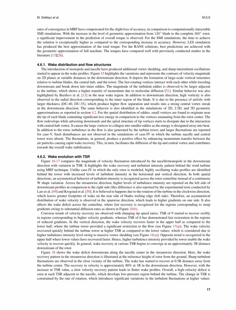
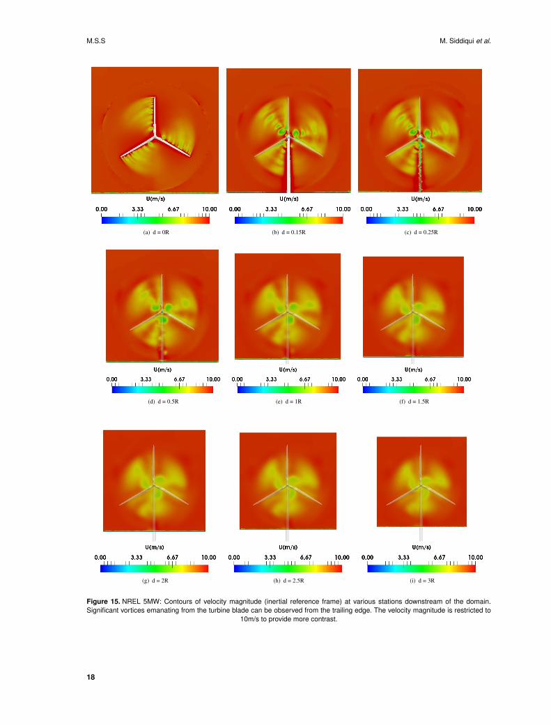
started to appear in the wake profiles. Figure 15 highlights the variations and represents the contours of velocity magnitudeon 2D planes at variable distances in the downstream direction. It depicts the formation of large-scale vortical structuresrelative to turbine blades, the central hub, and the tower. The fast rotating vortices interact with each other while travelingdownstream and break down into tinier eddies. The magnitude of the turbulent eddies is observed to be larger adjacentto the turbine, which shows a higher transfer of momentum due to molecular diffusion [51]. Similar behavior was alsohighlighted by Bazilevs et al. [13] in the near wake region. In addition to downstream direction, high vorticity is alsoobserved in the radial direction corresponding to the inner region of the blade. It is due to the presence of airfoils withlarger thickness (DU-40, DU-35), which produce higher flow separation and results into a strong central vortex streakin the downstream direction. The same behavior is also identified in the simulations of 2D, 2.5D, and 3D geometricapproximations as reported in section 4.2. For the spatial distribution of eddies, small vortices are found to originate nearthe tip of each blade containing significant less energy in comparison to the vortices emanating from the rotor center. Theflow redevelops while advecting downwards and the spiral structure of tip vortices starts to dissipate due to the interactionwith central hub vortex. It causes the large vortices to collapse into smaller eddies as the energy is dissipated away into heat.In addition to the rotor, turbulence in the flow is also generated by the turbine tower, and larger fluctuations are reportedfor case-V. Such disturbances are not observed in the simulations of case-IV in which the turbine nacelle and centraltower were absent. The fluctuations, in general, produce a positive effect by enhancing momentum transfer between theair particles causing rapid wake recovery. This, in turn, facilitates the diffusion of the tip and central vortex and contributestowards the overall wake stabilization.

4.6.2. Wake evolution with TSRFigure 16-17 compares the magnitude of velocity fluctuation introduced by the nacelle/monopole in the downstream

direction with variation in TSR. It highlights the wake recovery and turbulent intensity pattern behind the wind turbineusing MRF technique. Unlike case-IV in which the only rotor is modeled, highly oscillating wake profiles are identifiedbehind the tower with increased levels of turbulent intensity in the horizontal and vertical direction. In both spatialdirections, an asymmetrical behavior of turbulent intensity is recognized across the rotor centerline instead of a continuousW shape variation. Across the streamwise direction, higher levels of turbulence intensity are reported on the left side ofdownstream profiles in comparison to the right side (this difference is also reported by the experimental tests conducted byLars et al. [49] and Krogstad et al. [50]. It is believed to happens due to the rotation of the turbine in the clockwise direction,which leaves greater footprints of wake on the rear side of blades trailing edge (left side). Therefore, an asymmetricaldistribution of wake velocity is observed in the spanwise direction, which leads to higher gradients on one side. It alsoaffects the wake deficit across the centerline, where fast recovery is recognized for the regions corresponding to steepgradients owing to substantial diffusion rates as shown in Figure 16(b).

Converse trends of velocity recovery are observed with changing tip speed ratios. TSR of 9 started to recover swiftlyin regions corresponding to higher velocity gradients, whereas TSR of 6 has demonstrated fast restoration in the regionsof reduced gradients. In the vertical direction, the wake velocity recovers faster in the upper half as compared to thelower half, where the turbine tower provided a significant restriction to the flow (see Figure 17(a)). The wake velocityrecovered quickly behind the turbine tower at higher TSR as compared to the lower values, which is considered due tohigher turbulence intensity level owing to massive vortex shedding (see Figure 16(a)). Opposite trend is recognized in theupper half where lower values have recovered faster. Hence, higher turbulence intensity provided by tower enable the wakevelocity to recover quickly. In general, wake recovery at various TSR begins to converge at an approximately 3R distancedownstream of the rotor.

Figure 18 shows the wake deficit downstream along the nacelle center in the streamwise direction. Here, the wakerecovery pattern in the streamwise direction is illustrated at the reference height of rotor from the ground. Sharp turbulentfluctuations are observed in the close vicinity of the turbine. The wake has started to recover at 0.5R distance away fromthe turbine center. The recovery in velocity is approximately 80% at 1R in the downstream direction. However, with theincrease in TSR value, a slow velocity recovery pattern leads to flatter wake profiles. Overall, a high-velocity deficit isseen at each TSR adjacent to the nacelle, which develops low-pressure region behind the turbine. The change in TSR isconstrained by the rate of rotation, which introduces significant variations in the turbulent fluctuations at higher values.

17


(a) d = 0R (b) d = 0.15R (c) d = 0.25R

(d) d = 0.5R (e) d = 1R (f) d = 1.5R

(g) d = 2R (h) d = 2.5R (i) d = 3R

Figure 15. NREL 5MW: Contours of velocity magnitude (inertial reference frame) at various stations downstream of the domain.Significant vortices emanating from the turbine blade can be observed from the trailing edge. The velocity magnitude is restricted to

10m/s to provide more contrast.

18


0 1 2 3 4 5 6 71-U/Uref

1.0

0.5

0.0

0.5

z/R

(a) NREL 5MW: Wake deficit in vertical direction

0 1 2 3 4 5 61-U/Uref

0.4

0.2

0.0

0.2

0.4

0.6

y/R

(b) NREL 5MW: Wake deficit in horizontal direction

Figure 16. NREL 5MW: Wake deficit for variable TSR and at locations (0.15R, 0.30R, 0.45R, 0.60R, 0.90R, 1.30R, 2.00R, 2.50R,3.00R from hub). (–) TSR=6, (- -) TSR=7.5, (.) TSR=9; Note*: Successive profiles have been offset for better clarity.

0 2 4 6 8 10I/Iinf

1.0

0.5

0.0

0.5

z/R

(a) NREL 5MW: Turbulent intensity (I/Iinf ) in vertical direction

0 2 4 6 8 10I/Iinf

0.6

0.4

0.2

0.0

0.2

0.4

0.6

0.8

1.0y/

R

(b) NREL 5MW: Turbulent intensity (I/Iinf ) in horizontal direction

Figure 17. NREL 5MW: Turbulent for variable TSR and at locations (0.15R, 0.30R, 0.45R, 0.60R, 0.90R, 1.30R, 2.00R, 2.50R, 3.00Rfrom hub). (–) TSR=6, (- -) TSR=7.5, (.)TSR=9; Note*: Successive profiles have been offset for better clarity.

Such variations are instantly reflected in the wake recovery pattern in the streamwise direction. For all TSR, the recovery invelocity is delayed beyond 0.8R downstream. Considering the limited size of the present computational domain, completerecovery in velocity field could not be achieved.

5. CONCLUSION

A complete aerodynamics analysis of NREL 5MW wind turbine at full scale was conducted with an incremental level ofgeometric approximations (from simple 2D to complete 3D). Reynolds Averaged Navier Stokes (RANS) technique wasadopted with Sliding Mesh Interface (SMI), and Multiple Reference Frame (MRF) approaches to model the rotationaleffects present inside the turbine. Due to unavailability of experimental data for validation purpose at full scale, werestricted ourself to data from wind tunnel experiments involving sectional blade profiles or numerical/analytical resultsalready published in the literature for quantitative validations. However, wherever possible we tried to relate it to

19


0.4 0.6 0.8 1.0 1.2 1.4x/R

0.1

0.2

0.3

0.4

0.5

0.6

0.7

0.8

0.9

1-U

/Uref

TSR=6TSR=7.5TSR=9

Figure 18. NREL 5MW: Wake deficit behind the full machine using MRF along the centerline of the hub at the 90m height from theground.

experimental observation at wind tunnel scales, the best example being of the Cl, Cd vs. α at various segments alongthe blades span. Here we enumerate some of the important conclusions drawn from the study:

• For the turbine blade segments along the span, there is an optimal angle of attack (α) at which lift coefficienthas a maximum value. Below this α, the flow becomes parallel and hence the lift contributions from the top, andbottom surfaces offset each other resulting in a reduced overall torque. Whereas, above the optimal α, massiveflow separation results in the stall which contributes poorly to lift coefficient and produce lower torque. Theseobservations were highlighted in the contours of pressure superimposed with velocity at variable TSR whichcaptured the behavior extremely well.

• Regarding, flow dimensional characteristics, the flow closer to the hub is dominated by complex 3D structures,while as one recedes away from the center, the flow starts to lose its 3D characteristics and can be reasonably wellrepresented by efficient 2D simulations. In this work, an additional geometric approximation is also introduced andcoined 2.5D. It was shown that 2.5D modeling approach efficiently captures the underlying flow dynamics at aparticular flow cross-section with tapering effect in a reasonable time frame. Thus, for megawatt-size wind machineblades, 2D simulations should only be employed to identify the aerodynamic loading in the outer sections of blades.Whereas, 2.5D modeling strategy may work adequately near the hub where three-dimensional effects dominate andshould be resolved to get a real sense of flow field.

• MRF methodology has slightly overpredicted torque values as compared to the SMI simulations at each levelof geometrical approximation. A comparative study between 120 blade sector, 360 simple rotor and 360 fullmachine has highlighted an error of 10%, 5.6% and 4% respectively from the BEM results published in the literature.

• An unsymmetrical distribution of wake velocity is observed in the horizontal direction instead of a continuousW shape curve. Higher velocity gradients are observed on the trailing edge side of the blade, which resulted inuneven wake recovery pattern across the rotor centerline. Moreover, turbulence created by the support structureallowed swift velocity recovery, as enhanced molecular diffusion causes massive turbulent fluctuations to settledown rapidly.

• Velocity recovery at various tip speeds started to converge far downstream of the turbine. The deficit in the velocityis high for the low tip speed ratios as compared to the larger ones. The axial velocity recovery at the hub heightis approximately 75% at around 1R distance downstream. Flow visualization has exhibited a flow pattern of threelarge eddies originating from the turbine blades, which get dissipated by the interaction with eddies emanating fromthe turbine tower and nacelle at around 3R distance downstream.

• Geometric approximations employed in a numerical framework for the prediction of the aerodynamic characteristicin a megawatt-size wind turbine is sensitive and prone to the type of analysis in hand. If computational resources

20


are limited, and the full-scale 3D solution cannot be adopted, a 2.5D spatial dimension as introduced in the presentarticle should be preferred rather then performing a simplistic 2D analysis. Cyclic periodicity (120) can become alegitimate alternative if turbine’s overall torque calculations are under consideration. Whereas, if the purpose is toevaluate the horizontal wake deficit profiles in the downstream direction, (360) rotor sector can produce plausibleresults. However, for vertical profiles, nacelle and tower should be employed to get a realistic picture of the wake inthe downstream direction.

To improve the understanding of flow characteristics behind a rotating turbine, there is a need to validate the methodologiesas presented in the present manuscript against experimental results. In the current work, a RANS based k − ω SSTturbulence model is used. Although this model is known to be appropriate for simulations dominated by flow separation,still future studies are required using Large Eddy Simulations. When it comes to the simulation of wind turbines in a windfarm, even the MRF approach will be computationally expensive. There will be a need for employing simpler models basedon Strip Theory, and the evaluation of their computational efficiencies and accuracies in comparison to SMI and MRF willalso be undertaken in future works.

ACKNOWLEDGMENTS

The authors acknowledge the financial support from the Norwegian Research Council and the industrial part-ners of NOWITECH: Norwegian Research Centre for Offshore Wind Technology (Grant No.:193823/S60)(http://www.nowitech.no) and FSI-WT (Grant No.:216465/E20)(http://www.fsi-wt.no). Furthermore, the authorsgreatly acknowledge the Norwegian Metacenter for computational science (NOTUR-reference number:NN9322K/1589)(www.notur.no) for giving us access to the Vilje high-performance computer at the NorwegianUniversity of Science and Technology (NTNU).

REFERENCES

1. Tabib M, Rasheed A, Kvamsdal T. Investigation of the impact of wakes and stratification on the performance of anonshore wind farm. Energy Procedia 2015; 80:302 – 311.

2. Siddiqui MS, Rasheed A, Kvamsdal T, Tabib M. Effect of turbulence intensity on the performance of an offshorevertical axis wind turbine. Energy Procedia 2015; 80:312–320.

3. Bai CJ, Wang WC. Review of computational and experimental approaches to analysis of aerodynamic performancein horizontal-axis wind turbines. Renewable and Sustainable Energy Reviews 2016; 63:506–519.

4. Yang H, Shen W, Xu H, Hong Z, Liu C. Prediction of the wind turbine performance by using BEM with airfoil dataextracted from CFD. Renewable Energy 2014; 70(0):107–115.

5. Monteiro JP, Silvestre MR, Piggott H, Andre JC. Wind tunnel testing of a horizontal axis wind turbine rotor andcomparison with simulations from two blade element momentum codes. Journal of Wind Engineering and IndustrialAerodynamics 2013; 123:99–106.

6. Bottasso CL, Campagnolo F, Petrovic V. Wind tunnel testing of scaled wind turbine models: Beyond aerodynamics.Journal of Wind Engineering and Industrial Aerodynamics 2014; 127(0):11–28.

7. Miller A, Chang B, Issa R, Chen G. Review of computer-aided numerical simulation in wind energy. Renewable andSustainable Energy Reviews 2013; 25(0):122–134.

8. Siddiqui MS, Durrani N, Akhtar I. Quantification of the effects of geometric approximations on the performance of avertical axis wind turbine. Renewable Energy 2015; 74(0):661–670.

9. Devinant PH, Laverne T, Hureau J. Experimental study of wind turbine airfoil aerodynamics in high turbulence.Journal of Wind Engineering and Industrial 2002; 90:689–707.

10. Christophe S, Aubrun S, Loyer S, Devinant P. Unsteady characteristics of the static stall of an airfoil subjected tofreestream turbulence level up to 16%. Experiments in Fluids 2006; 41(4):641–648.

11. Tangler JL. Insight into wind turbine stall and post-stall aerodynamics. Wind Energy 2004; 7(3):247–260.12. Spentzos A, Barakos GN, Badcock KJ, Richards BE, Wernert P, Schreck S, Raffel M. Investigation of three-

dimensional dynamic stall using computational fluid dynamics. Journal of American Institute of Aeronautics andAstronautics, AIAA 2005; 43:1023–1033.

13. Yu G, Shen X, Zhu X, Du Z. An insight into the separate flow and stall delay for HAWT. Renewable Energy 2011;36(1):69–76.

14. Troldborg N, Zahle F, Sørensen NN. Simulation of a MW rotor equipped with vortex generators using CFD and anactuator shape model. Proceedings of 53rd AIAA Aerospace Sciences Meeting, American Institute of Aeronautics &Astronautics 2015; .

21


15. Sørensen NN, Zahle F. Simulations of wind turbine rotor with vortex generators. Journal of Physics: ConferenceSeries (Online) 2016; 753.

16. Guntur S, Sørensen NN, Schreck S, Bergami L. Modeling dynamic stall on wind turbine blades under rotationallyaugmented flow fields. Wind Energy 2016; 19(3):383397.

17. Cavar D, Rethore PE, Bechmann A, Sørensen N, Martinez B, Zahle F, Berg J, Kelly M. Comparison of openfoamand ellipsys3D for neutral atmospheric flow over complex terrain. Wind Energy Science Discussions 2016; 1:5570.

18. Bazilevs Y, Hsu MC, Akkerman I, Wright S, Takizawa K, Henicke B, Spielman T, Tezduyar TE. 3D simulation ofwind turbine rotors at full scale. part I: Geometry modeling and aerodynamics. International Journal for NumericalMethods in Fluids 2011; 65(1-3):207–235.

19. Hsu MC, Bazilevs Y. Fluid–structure interaction modeling of wind turbines: simulating the full machine.Computational Mechanics 2012; 50(6):821–833.

20. Bazilevs Y, Hsu MC, Kiendl J, Benson D. A computational procedure for prebending of wind turbine blades.International Journal for Numerical Methods in Engineering 2012; 89(3):323–336.

21. Hsu MC, Akkerman I, Bazilevs Y. Finite element simulation of wind turbine aerodynamics: validation study usingNREL phase VI experiment. Wind Energy 2014; 17(3):461–481.

22. Jonkman J, Marshal L, Buhl J. Fast users guide. National Renewable Energy Laboratory, Golden, CO, 2005, TechRep NREL/EL-500-38230; .

23. Siddiqui MS, Rasheed A, Tabib M, Kvamsdal T. Numerical analysis of NREL 5MW wind turbine: A study towards abetter understanding of wake characteristic and torque generation mechanism. Journal of Physics: Conference Series2016; 753(3):032 059.

24. Zhong H, Du P, Tang F, Wang L. Lagrangian dynamic large-eddy simulation of wind turbine near wakes combinedwith an actuator line method. Applied Energy 2015; 144(0):224–233.

25. Jasak H. Dynamic mesh handling in OpenFOAM. 47th AIAA Aerospace Sciences Meeting Including the NewHorizons Forum and Aerospace Exposition 5-8 January, 2008; 52:(AIAA 2009–341).

26. Jonkman JM, Butterfield S, Musial W, Scott G. Definition of a 5MW reference wind turbine for offshore systemdevelopment. National Renewable Energy Laboratory 2009, Tech Rep NREL/TP-500e38060; .

27. Khalid S, Rabbani T, Akhtar I, Durrani N, Siddiqui MS. Reduced-order modeling of torque on a vertical-axis windturbine at varying tip-speed ratios. ASME Journal of Computational and Nonlinear Dynamics 2015; 10(CND-14-1055):041 012(9).

28. Bak C, Timmer W. Aerodynamic characteristics of wind turbine blade airfoils. Advances in wind turbine blade designand materials, Woodhead Publishing, 2013.

29. Timmer WA, Van Rooij RPJOM. Summary of the delft university wind turbine dedicated airfoils. Journal of SolarEnergy Engineering 2003; 125:488–496.

30. Siddiqui MS, Durrani N, Akhtar I. Numerical study to quantify the effects of struts and central hub on the performanceof a three dimensional vertical axis wind turbine using sliding mesh. ASME Power Conference 2013; 2(POWER2013-98300):V002T09A020(11).

31. Mo JO, Choudhry A, Arjomandi M, Lee YH. Large eddy simulation of the wind turbine wake characteristics in thenumerical wind tunnel model. Journal of Wind Engineering and Industrial Aerodynamics 2013; 112:11–24.

32. Siddiqui MS, Ahmed H, Ahmed S. Numerical simulation of a compressed air driven tesla turbine. ASME PowerConference 2014; 2(POWER2014-32069):V002T09A009(6).

33. Spalart P, Allmaras S. A one-equation turbulence model for aerodynamic flows. AIAA Paper 92-0439(1992) ; .34. Tachos NS, Filios AE, Margaris DP. A comparative numerical study of four turbulence models for the prediction

of horizontal axis wind turbine flow. Proceedings of the Institution of Mechanical Engineers, Part C: Journal ofMechanical Engineering Science 2010; 224(9):1973–1979.

35. Menter F. Review of the shear-stress transport turbulence model experience from an industrial perspective.International Journal of Computational Fluid Dynamics 2009; 23:305–316.

36. Nordanger K, Holdahl R, Kvarving AM, Rasheed A, Kvamsdal T. Implementation and comparison of threeisogeometric Navier-Stokes solvers applied to simulation of flow past a fixed 2D NACA0012 airfoil at high Reynoldsnumber. Computer Methods in Applied Mechanics and Engineering 2015; 284:664–688.

37. Nordanger K, Holdahl R, Kvamsdal T, Kvarving AM, Rasheed A. Simulation of airflow past a 2D NACA0015 airfoilusing an isogeometric incompressible Navier-Stokes solver with the Spalart-Allmaras turbulence model. ComputerMethods in Applied Mechanics and Engineering 2015; 290:183 – 208.

38. Sarlak Chivaee H, Nishino T, Sørensen J. URANS simulations of separated flow with stall cells over an NREL S826airfoil. A I P Conference Proceedings Series 2016; 1738.

39. Herraez I, Akay B, van Bussel GJW, Peinke J, Stoevesandt B. Detailed analysis of the blade root flow of a horizontalaxis wind turbine. Wind Energy Science 2016; 1(2):89–100.

40. Bazilevs Y, Hsu MC, Scott M. Isogeometric fluidstructure interaction analysis with emphasis on non-matchingdiscretizations, and with application to wind turbines. Computer Methods in Applied Mechanics and Engineering

22


2012; 249-252(0):28–41. Higher Order Finite Element and Isogeometric Methods.41. Zahle F, Bak C, Sørensen N, Guntur S, Troldborg N. Comprehensive Aerodynamic Analysis of a 10MW Wind Turbine

Rotor Using 3D CFD. American Society of Mechanical Engineers, 2014.42. Sørensen NN, Bechmann A, Boudreault LE, Koblitz T, Sogachev A. CFD applications in wind energy using RANS.

von Karman Institute for Fluid Dynamics, 2013.43. Wilcox D. Simulation of transition with a two-equation turbulence model. AIAA Journal. 32 1994; :247–255.44. Jasak H. Error analysis and estimation in the finite volume method with applications to fluid flows. Imperial College,

University of London 1996; .45. Kooijman HJT, Lindenburg C, Winkelaar D, , Hooft ELVD. DOWEC 6MW pre-design: Aero-elastic modeling of

the dowec 6MW pre-design in phatas,. DOWEC Dutch Offshore Wind Energy Converter 19972003 Public Reports ,DOWEC 10046-009, ECN-CX–01-135, Petten, the Netherlands: Energy Research Center of the Netherlands 2003; .

46. Akay B, Micallef D, Ferreira CJS, van Bussel GJW. Effects of geometry and tip speed ratio on the hawt blade’s rootflow. Journal of Physics: Conference Series 2014; 555(1):012 002.

47. The norwegian metacenter for computational science (NOTUR). http://www.sigma2.no. [Online; accessed26-September-2016].

48. Ivanell S, Sørensen JN, Mikkelsen R, Henningson D. Numerical analysis of the tip and root vortex position in thewake of a wind turbine. Journal of Physics: Conference Series 2007; 75(1):012 035.

49. Krogstad PA, Sætran L. An experimental and numerical study of the performance of a model turbine. Wind Energy2012; 15(3):443–457.

50. Krogstad PA, Sætran L, Adaramola MS. Blind test 3 calculations of the performance and wake development behindtwo inline and offset model wind turbines. Journal of Fluids and Structures 2015; 52:65–80.

51. Ainslie J. Calculating the flow field in the wake of wind turbines. Journal of Wind Engineering and IndustrialAerodynamics 1988; 27(1-3):213–224.

23

http://www.sigma2.no

Numerical investigation of modeling frameworks and ...

Documents

Transcript of Numerical investigation of modeling frameworks and ...