Scuola Dottorale di Ingegneria

sezione di Ingegneria Meccanica e Industriale

XXI Ciclo

“Numerical analysis of the hydrogen

combustion in a double cavity Trapped

Vortex Combustor”

PhD thesis by Alessandro Di Marco

Advisor: Prof. R. Camussi

PhD Coordinator: Prof. E. Bemporad

Degree of

Doctor of Philosophy March 2009

In Memory of Prof. G. Guj (R.I.P.)

2

Contents

Abstract...................................................................................................... 5 List of symbols........................................................................................... 6 1 Introduction......................................................................................... 9

1.1 Background and motivations........................................................................... 9 1.2 Structure of the thesis .................................................................................... 10

2 Theoretical Background................................................................... 11 2.1 Review of some property relations ................................................................ 11

2.1.1 Ideal-Gas Mixtures ....................................................................................................11 2.1.2 Stoichiometry .............................................................................................................12 2.1.3 Hydrogen properties ..................................................................................................13

2.2 Principles of combustion ............................................................................... 14 2.2.1 Conservation equations for multicomponent reacting systems..................................14 2.2.2 Dimensionless governing parameters........................................................................20 2.2.3 Basic flame types........................................................................................................21

2.2.3.1 Premixed Flames............................................................................................................................. 22 2.2.3.2 Non-premixed flames....................................................................................................................... 26

2.3 Chemical kinetics and reaction mechanisms................................................. 28 2.3.1 Rates of reactions.......................................................................................................29 2.3.2 Hydrogen Chemical Mechanism................................................................................30 2.3.3 Oxides of nitrogen formation .....................................................................................33

2.4 Mild Combustion ........................................................................................... 34 3 Trapped Vortex Combustor............................................................. 36

3.1 TVC concept................................................................................................... 37 3.2 TVC Development.......................................................................................... 40

3.2.1 Air Force Research Laboratory.................................................................................40 3.2.2 General Electric Company.........................................................................................41 3.2.3 DOE National Energy Technology Laboratory .........................................................42 3.2.4 Ramgen Power Systems (RPS)...................................................................................43 3.2.5 ALM Turbines ............................................................................................................44

3.3 ENEA TVC Geometry .................................................................................... 45 4 Numerical Combustion Modelization ............................................. 49

4.1 Computational domain and mesh properties ................................................ 49 4.2 Numerical model............................................................................................ 53

4.2.1 Realizable k-ε .............................................................................................................54 4.2.2 Radiation model .........................................................................................................55 4.2.3 Combustion Model .....................................................................................................58 4.2.4 Gas Mixture Properties..............................................................................................59 4.2.5 Boundary conditions ..................................................................................................61

5 Results ................................................................................................ 62 5.1 Test Matrix..................................................................................................... 62 5.2 Flow field and flame ...................................................................................... 63 5.3 Effect of moisture........................................................................................... 72 5.4 Effect of the primary and secondary equivalence ratio ................................ 76

3

5.5 Combustion instabilities ................................................................................ 79 6 Conclusions and future perspectives ............................................... 96 References................................................................................................ 98 Appendix................................................................................................ 101

4

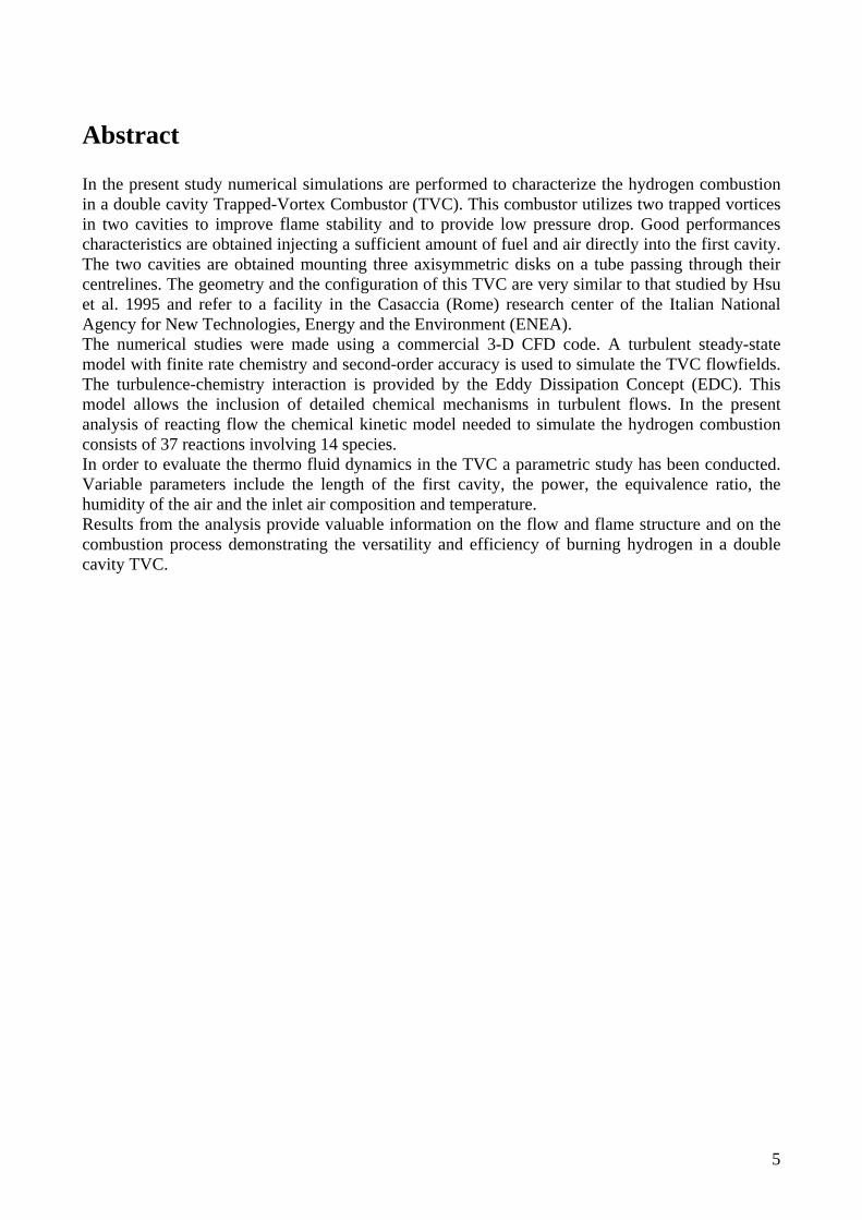
Abstract In the present study numerical simulations are performed to characterize the hydrogen combustion in a double cavity Trapped-Vortex Combustor (TVC). This combustor utilizes two trapped vortices in two cavities to improve flame stability and to provide low pressure drop. Good performances characteristics are obtained injecting a sufficient amount of fuel and air directly into the first cavity. The two cavities are obtained mounting three axisymmetric disks on a tube passing through their centrelines. The geometry and the configuration of this TVC are very similar to that studied by Hsu et al. 1995 and refer to a facility in the Casaccia (Rome) research center of the Italian National Agency for New Technologies, Energy and the Environment (ENEA). The numerical studies were made using a commercial 3-D CFD code. A turbulent steady-state model with finite rate chemistry and second-order accuracy is used to simulate the TVC flowfields. The turbulence-chemistry interaction is provided by the Eddy Dissipation Concept (EDC). This model allows the inclusion of detailed chemical mechanisms in turbulent flows. In the present analysis of reacting flow the chemical kinetic model needed to simulate the hydrogen combustion consists of 37 reactions involving 14 species. In order to evaluate the thermo fluid dynamics in the TVC a parametric study has been conducted. Variable parameters include the length of the first cavity, the power, the equivalence ratio, the humidity of the air and the inlet air composition and temperature. Results from the analysis provide valuable information on the flow and flame structure and on the combustion process demonstrating the versatility and efficiency of burning hydrogen in a double cavity TVC.

5

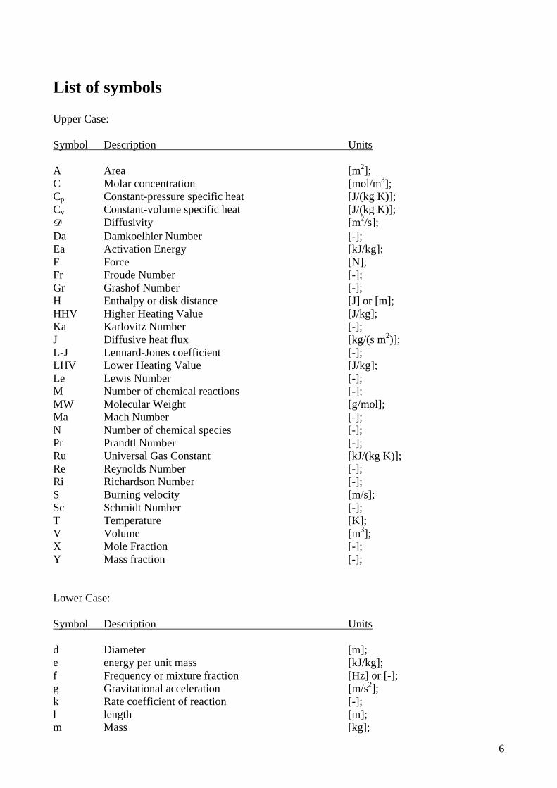
List of symbols Upper Case: Symbol Description Units A Area [m2]; C Molar concentration [mol/m3]; Cp Constant-pressure specific heat [J/(kg K)]; Cv Constant-volume specific heat [J/(kg K)]; D Diffusivity [m2/s]; Da Damkoelhler Number [-]; Ea Activation Energy [kJ/kg]; F Force [N]; Fr Froude Number [-]; Gr Grashof Number [-]; H Enthalpy or disk distance [J] or [m]; HHV Higher Heating Value [J/kg]; Ka Karlovitz Number [-]; J Diffusive heat flux [kg/(s m2)]; L-J Lennard-Jones coefficient [-]; LHV Lower Heating Value [J/kg]; Le Lewis Number [-]; M Number of chemical reactions [-]; MW Molecular Weight [g/mol]; Ma Mach Number [-]; N Number of chemical species [-]; Pr Prandtl Number [-]; Ru Universal Gas Constant [kJ/(kg K)]; Re Reynolds Number [-]; Ri Richardson Number [-]; S Burning velocity [m/s]; Sc Schmidt Number [-]; T Temperature [K]; V Volume [m3]; X Mole Fraction [-]; Y Mass fraction [-]; Lower Case: Symbol Description Units d Diameter [m]; e energy per unit mass [kJ/kg]; f Frequency or mixture fraction [Hz] or [-]; g Gravitational acceleration [m/s2]; k Rate coefficient of reaction [-]; l length [m]; m Mass [kg];

6

t Time [s]; p Pressure [Pa]; q Heat Flux [W/m2], r,θ,z Cylindrical coordinate system [m,° or rad,m]; u velocity component in x- or axial direction [m/s]; v velocity component y- or radial direction [m/s]; w velocity component z-direction [m/s]; x,y,z Cartesian coordinate system [m]; Greek symbols: Symbol Description Units α Thermal diffusivity [m2/s]; δ Thickness [m]; ε Dissipation rate of turbulent kinetic energy [m/s3]; Φ Equivalence ratio [-]; κ Turbulent kinetic energy [m2/s2]; λ Thermal conductivity [J/(s m K)]; μ Dynamic viscosity [N s/m2]; ν Kinematic viscosity [m2/s]; ρ Density [kg/m3]; σ Normal stress [N/m2]; τ Shear stress [N/m2]; ω Mass rate of production of species [kg/(s m3)]; Ω Vorticity [rad/s]; Acronyms: Symbol Description _____ AFRL Air Force Research Laboratory; APU Auxiliary Power Unit; ATS Advanced Turbine System; AVC Advanced Vortex Combustion; CEC California Energy Commission; DLN Dry Lean NOx; DOE Department Of Energy; EDC Eddy Dissipation Concept; GE General Electric; ICAO International Civil Aviation Organization; IGCC Integrated Gasification Combined Cycle; LES Large Eddy Simulation; LBO Lean Blow Out; LECTR Low Emission Combustion Test and Research; NETL National Energy Technology Laboratory; PSR Perfect stirred Reactor; RPS Ramgen Power Systems;

7

RQL Rich-burn, Quick-mix/quench, Lean burn; SERDP Strategic Environmental Research and Development Program; TVC Trapped Vortex Combustor; WSGGM Weighted Sum of Gray Gases Model.

8

1 Introduction

1.1 Background and motivations Combustion is a subject of great relevance from the scientific and technological point of view. The scientific interest is associated with the variety of physical processes which are encountered and with the inherent multi-disciplinary character of the subject, which involves Fluid Mechanics, Chemistry, Thermodynamics and the environmental science. The technological relevance is instead associated with the vast spectrum of industrial and engineering applications in which combustion is used. In almost all cases, chemical reactions, i.e. the combustion process, through which heat is produced, develop within a turbulent flow field. The characteristics and the evolution of the combustion process is strictly dependent on the property of the turbulent field and on the way fuel and oxidizer are mixed. The state of the mixedness of the reactants divides the combustion, and the flames, in two classes: premixed and non-premixed (or diffusive). In a premixed combustion fuel and oxidizer are mixed at the molecular level prior to the occurrence of any significant chemical reaction. Contrarily, in a diffusion combustion, the reactants are initially separated, and reaction occurs only at the interface between the fuel and the oxidizer, where mixing and reaction both take place. In both classes of flames, depending on the combustion device’s operating range, important design criteria are the avoidance of flashback and liftoff, two conditions of instability. Flashback occurs when the flame enters and propagates through the burner tube or port without quenching; while liftoff is the condition where the flame is not attached to the burner tube or port hub, rather, is stabilized at some distance from the port. A poor stability of the flame can be obtained attempting to burn fuel in lean mixture combustion regimes to reduce the consumption or the pollutant emissions (furnaces, aircraft engines, turbo-reactors, etc.). Combustion stability is often achieved through the use of recirculation zones to provide a continuous ignition source which facilitates the mixing of hot combustion products with the incoming fuel and air mixture. Swirl vanes, bluff bodies and rearward facing steps are commonly employed to establish recirculation zones for flame stability. Each method creates a low velocity zone of sufficient residence time and turbulence levels such that the combustion process becomes self-sustaining. The challenge, however, is the selection of a flame stabilizer which ensures both performance (emissions, combustor acoustic and pattern factor) and cost goals are met. As opposed to conventional combustion systems which rely on swirl stabilization, the TVC employs cavities to stabilize the flame and grows from the wealth of literature on cavity flows [Hsu et al., 1995, Sturgess and Hsu, 1997, Straub et al., 2000, Roquemore et al., 2001]. Much of this effort examines the flow field dynamics established by the cavities, as demonstrated in aircraft wheel wells, bomb bay doors and other external cavity structures. Cavities have also been studied as a means of cooling and reducing drag on projectiles and for scramjets and waste incineration [Gharib and Roshko, 1987]. Very little work, however, exists on studying cavity flameholders for subsonic flow [Roquemore et al., 2001]. and none at all for lean premixed operation for potential use in a land based gas turbine engine The actual stabilization mechanism facilitated by the TVC is relatively simple. A conventional bluff or fore body is located upstream of a smaller bluff body - commonly referred to as an aft body - at a prescribed distance commensurate with cold flow stabilization studies [Hsu et al., 1995, Sturgess and Hsu, 1997, Roquemore et al., 2001]. The flow issuing from around the first bluff body separates as normal, but instead of developing shear layer instabilities which in most circumstances is the prime mechanism for initiating blowout, the alternating array of vortices are conveniently trapped

9

or locked between the two bodies. The very stable yet more energetic primary/core flame zone is now very resistant to external flow field perturbations, yielding extended lean and rich blowout limits relative to its simple bluff body counterpart. Due to its configuration, the system has greater flame holding surface area and hence will facilitate a more compact primary/core flame zone; which is essential in promoting high combustion efficiency and reduced emissions. Incorporation of transverse struts (Roquemore et al., 2001), which enhance the mixing/interaction of hot combustion products with the cooler premixed fuel and air, further reinforces the merits of the TVC as an excellent candidate for a lean-premixed combustion system. Furthermore, since part of combustion occurs within the recirculation zone, a typically flameless (Mild or Flox) regime can be achieved. The objectives of this thesis are the evaluation of the performances and the stability regimes of a double cavity TVC by means of numerical simulations. The simulations are performed with a commercial code since this combustor is used in the industrial field. Another aim of this research is to contribute to improve the knowledge and understanding of the physics involved in the TVC combustion and cover the lack of results regarding the use of hydrogen as fuel with this kind of combustor.

1.2 Structure of the thesis The approach taken writing the thesis is to present and discuss some of the theoretical and practical elements needed to understand the model used and to relate the results obtained to practical applications. The section 2 is structured to give all the fluid mechanics and thermochemistry fundamentals useful to a better comprehension of the arguments treated in the following sections. The section 3 contains a brief review of the TVC state of the art and development, followed by a description of the TVC geometry taken into consideration. Furthermore an outline of the TVC behaviour under certain working conditions is given. The numerical combustion modelization is described in section 4. It deals with a description of the approach used to solve the physical model needed to analyze the TVC performances. The computational domain and the mesh properties are first shown and then the main characteristic of the model with some reminds to the original articles/books to gather further information are given. Finally, in section 5 and 6 the results of the simulations and discussion are presented. The results are ordered following the phenomenological consequences due to the variation of the variables reported in the test matrix.

10

2 Theoretical Background In this chapter, some important concepts related to combustion processes are examined. A review of some essential topics such as the basic properties of the ideal-gas mixtures, the stoichiometry and the thermo physical properties of the fuel (hydrogen) is briefly given. Successive paragraphs deal with the conservation equations for multicomponent reacting mixtures and relatives dimensionless governing parameters, the study of premixed and non-premixed flames and some basic chemical kinetics concepts. Then an outline of the elementary steps involved in the H2-O2 chemical mechanism and in the oxides of nitrogen formation is given. Details can be found in reference books [e.g. Kuo 1986, Williams 1985 …] so only the main concepts are summarized in the following.

2.1 Review of some property relations

2.1.1 Ideal-Gas Mixtures Two important and useful concepts used to characterize the composition of a mixture are the constituent mole fractions and mass fractions. Considering a multicomponent mixture of gases composed of N1 moles of species 1, N2 moles of species 2, etc.. the mole fraction of species i, Xi is defined as the fraction of the total number of moles in the system that are species:

tot

i

i

ii N

NNNN

NX =

++++=

......21

2-1

Similarly, the mass fraction of species i, Yi, is the amount of mass of species i compared with the total mixture mass:

tot

i

i

ii m

mmmm

mY =

++++=

......21

2-2

Mole fractions and mass fractions are readily converted from one to another using the molecular weights of the species of interest and of the mixture:

mix

iii MW

MWXY = ,

i

mixii MW

MWYX =

2-3

The partial pressure can be related to the mixture composition and total pressure as:

PXP ii = 2-4

For ideal gas mixtures, many mass- (or molar-) specific mixture properties are calculated simply as mass (or mole) fraction weighted sums of the individual species-specific properties. For example, mixture enthalpies are calculated as.

11

∑=

iiimix hYh , ∑=

iiimix hXh 2-5

2.1.2 Stoichiometry The stoichiometric quantity of oxidizer is just that amount needed to completely burn a quantity of fuel. If more than a stoichiometric quantity of oxidizer is supplied, the mixture is said to be fuel lean, or just lean; while supplying less than the stoichiometric oxidizer results in a fuel-rich, or rich mixture. The stoichiometric oxidizer- (or air-) fuel ratio (mass) is determined by writing simple atom balances, assuming that the fuel reacts to form an ideal set of products. For a hydrocarbon fuel given by CxHy, the stoichiometric relation can be expressed by the a global reaction mechanism (see 2.3) as

( ) 22222 76.32

76.3 aNOHyxCONOaHC yx ++→++ 2-6

Where

4yxa +=

It is assumed, in the following that the simplified composition for air is 21% O2 and 79% N2 (by volume) i.e. that for each mole of O2 in air, there are 3.76 moles of N2. The stoichiometric air-fuel ratio can be found as

fuel

air

stoicfuel

air

stoic MWMWa

mm

FA

176.4

=⎟⎟⎠

⎞⎜⎜⎝

⎛=⎟

⎠⎞

⎜⎝⎛ 2-7

Where MWair and MWfuel are the molecular weights of the air and the fuel, respectively. The equivalence ratio, Φ, is commonly used to indicate quantitatively whether a fuel-oxidizer mixture is rich, lean, or stoichiometric. The equivalence ratio is defined as

( )( )

( )( )

stoic

stoic

AF

AF

FAF

A==Φ 2-8

From the definition: For fuel-lean conditions, we have 0<Φ<1, For stoichiometric conditions, we have Φ=1, And for fuel-rich conditions, we have 1<Φ<∞.

12

2.1.3 Hydrogen properties Hydrogen is the fuel used in the simulations. In this section its main thermo physical properties are reported. At standard temperature and pressure, hydrogen is a colourless, odourless, non-metallic, tasteless, highly flammable diatomic gas. Dihydrogen (hydrogen gas) is highly flammable and will burn at concentrations of 4% or more H2 in air. The enthalpy of combustion for hydrogen is -286 kJ/mol; it burns according to the following global reaction:

( )molkJkJOHOH /28657222 222 +→+ 2-9 When mixed with oxygen across a wide range of proportions, hydrogen explodes upon ignition. Hydrogen burns violently in air. It ignites automatically at a temperature of 560°C. Pure hydrogen-oxygen flames burn in the ultraviolet colour range and are nearly invisible to the naked eye, as illustrated by the faintness of flame from the main Space Shuttle engines. Another characteristic of hydrogen fires is that the flames tend to ascend rapidly with the gas in air causing less damage than hydrocarbon fires. In the following tables the hydrogen main properties and a comparison with other fuels of the ignition and flammability properties are reported.

H2 Phase Gas Melting point [K] 14.01 Boiling point [K] 20.28 Heat of fusion [kJ/mol] 0.117 Heat of vaporization [kJ/mol] 0.904 Gas Constat R [kJ/kg K] 4.124 Density ρ (300 K) [kg/m3] 0.0819 Specific heat cp (300 K) [kJ/kg K] 14.307 Thermal conductivity k (300 K) [W/m °C] 0.182 Thermal diffusivity α [m2/s] 1.55E-04 Dynamic Viscosity μ [kg/m s] 8.90E-06 Higher Heating Value HHV [kJ/kg] 141850 Lower Heating value LHV [kJ/kg] 120010

Tab. 2-1: Hydrogen Thermo Physical properties.

H2 CH4 C3H8

Minimum ignition energy [mJ] 0.02 0.28 0.25 Ignition temperature [K] 858 810 783 Adiabatic flame temperature [K] 2384 2227 2268 Limits of flammability (% by volume in Air) 4.1-75 4.3-15 2.2-9.5 Maximum laminar flame velocity [cm/s] 270 38 40 Diffusivity [cm2/s] 0.63 0.2 Minimum quenching distance at 1 atm [cm] 0.06 0.25 0.19 Normalized flame emissivity (200 K and 1 atm) 1 1.7 1.7

Tab. 2-2: Ignition and flammability properties.

13

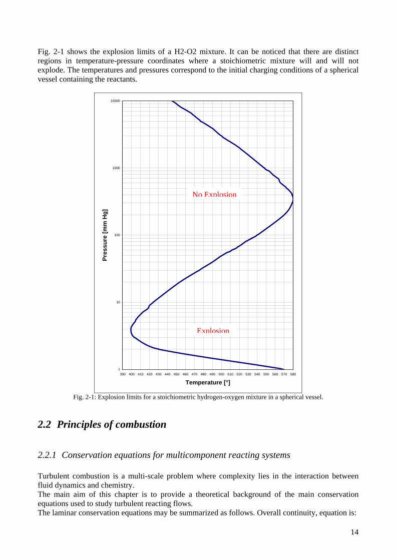
Fig. 2-1 shows the explosion limits of a H2-O2 mixture. It can be noticed that there are distinct regions in temperature-pressure coordinates where a stoichiometric mixture will and will not explode. The temperatures and pressures correspond to the initial charging conditions of a spherical vessel containing the reactants.

1

10

100

1000

10000

390 400 410 420 430 440 450 460 470 480 490 500 510 520 530 540 550 560 570 580

Temperature [°]

Pres

sure

[mm

Hg]

No Explosion

Explosion

Fig. 2-1: Explosion limits for a stoichiometric hydrogen-oxygen mixture in a spherical vessel.

2.2 Principles of combustion

2.2.1 Conservation equations for multicomponent reacting systems Turbulent combustion is a multi-scale problem where complexity lies in the interaction between fluid dynamics and chemistry. The main aim of this chapter is to provide a theoretical background of the main conservation equations used to study turbulent reacting flows. The laminar conservation equations may be summarized as follows. Overall continuity, equation is:

14

0=⋅∇+∂∂ v

trρρ 2-10

Which is the equation of continuity for the mixture. For a multicomponent system the equation of continuity for a component i is:

iiiii VYYv

tY ωρρρ =⋅∇+∇⋅+

∂∂ rr 2-11

In a general multicomponent system there are N equations of this kind (or N-1 if the equation for the mixture is used). The addition of these equations gives the equation of continuity for the mixture. The ωi in each species continuity equation is determined by the phenomenological chemical kinetic expression (see sec. 2.3.1 for details):

( ) ∏∑==

⎟⎟⎠

⎞⎜⎜⎝

⎛−−=

N

j u

j

u

kak

M

kkikiii

kj

k

TRpX

TRE

TBW1

'

1,,

,

exp'''ν

αννω 2-12

Where M is the total number of chemical reactions occurring and N is the total number of chemical species present. For what concerns the partial differential momentum equation, the basic assumption is that we are dealing with continuous, isotropic, and homogeneous media. We shall consider the special case of a Newtonian fluid, that is, a fluid exhibiting a linear relationship between shear stress and rate of deformation, resulting in the Navier-Stokes equation. The momentum equation in indicial notation is:

( )∑=

+∂∂

=⎥⎥⎦

⎤

⎢⎢⎣

⎡

∂∂

+∂∂ N

kikk

j

ji

j

ij

i fYxx

uutu

1ρ

σρ 2-13

σji is the stress tensor, fk is the force per unit mass on the k-th species. Substituting the constitutive equation:

⎟⎟⎠

⎞⎜⎜⎝

⎛

∂∂

+∂∂

+∂∂

⎟⎠⎞

⎜⎝⎛ −+−=

i

j

j

iij

k

kijij x

uxu

xup μδμμδσ

32' 2-14

in the momentum equation, we obtain the Navier-Stokes equation:

( )∑=

+⎥⎥⎦

⎤

⎢⎢⎣

⎡⎟⎟⎠

⎞⎜⎜⎝

⎛

∂∂

+∂∂

+∂∂

⎟⎠⎞

⎜⎝⎛ −+−

∂∂

=⎥⎥⎦

⎤

⎢⎢⎣

⎡

∂∂

+∂∂ N

kikk

i

j

j

iij

k

kij

jj

ij

i fYxu

xu

xup

xxuu

tu

132' ρμδμμδρ 2-15

Where μ’ is the bulk viscosity, μ is the dynamic viscosity. The difference

μμλ32'−=

15

is the second viscosity. The usual practice is to employ the hypothesis made by Stokes in 1845:

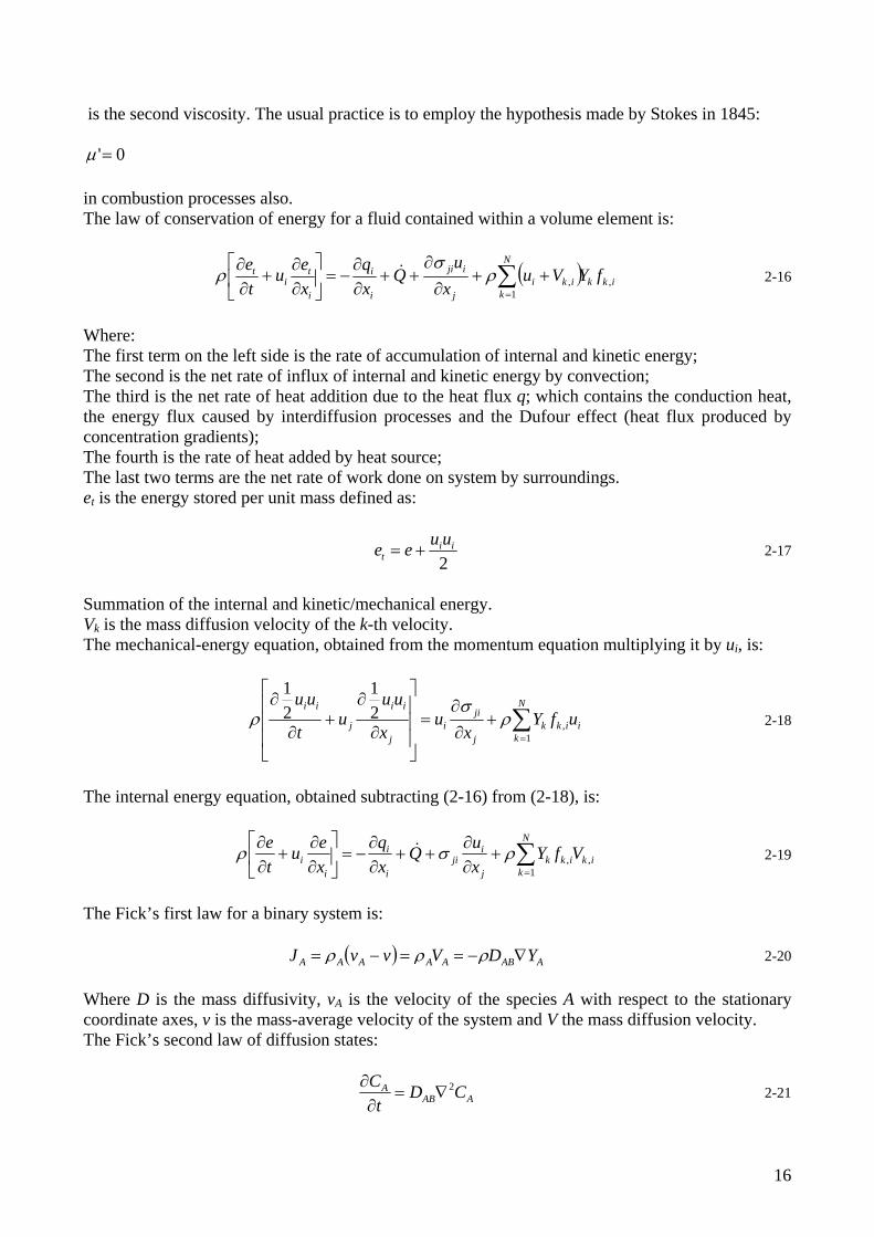
0'=μ in combustion processes also. The law of conservation of energy for a fluid contained within a volume element is:

( ) ikk

N

kiki

j

iji

i

i

i

ti

t fYVux

uQ

xq

xeu

te

,1

,∑=

++∂

∂++

∂∂

−=⎥⎦

⎤⎢⎣

⎡∂∂

+∂∂ ρ

σρ & 2-16

Where: The first term on the left side is the rate of accumulation of internal and kinetic energy; The second is the net rate of influx of internal and kinetic energy by convection; The third is the net rate of heat addition due to the heat flux q; which contains the conduction heat, the energy flux caused by interdiffusion processes and the Dufour effect (heat flux produced by concentration gradients); The fourth is the rate of heat added by heat source; The last two terms are the net rate of work done on system by surroundings. et is the energy stored per unit mass defined as:

2ii

tuuee += 2-17

Summation of the internal and kinetic/mechanical energy. Vk is the mass diffusion velocity of the k-th velocity. The mechanical-energy equation, obtained from the momentum equation multiplying it by ui, is:

∑=

+∂∂

=⎥⎥⎥

⎦

⎤

⎢⎢⎢

⎣

⎡

∂

∂+

∂

∂ N

kiikk

j

jii

j

ii

j

iiufY

xu

x

uuu

t

uu

1,

21

21

ρσ

ρ 2-18

The internal energy equation, obtained subtracting (2-16) from (2-18), is:

∑=

+∂∂

++∂∂

−=⎥⎦

⎤⎢⎣

⎡∂∂

+∂∂ N

kikikk

j

iji

i

i

ii VfY

xuQ

xq

xeu

te

1,,ρσρ & 2-19

The Fick’s first law for a binary system is:

( ) AABAAAAA YDVvvJ ∇−==−= ρρρ 2-20 Where D is the mass diffusivity, vA is the velocity of the species A with respect to the stationary coordinate axes, v is the mass-average velocity of the system and V the mass diffusion velocity. The Fick’s second law of diffusion states:

AABA CD

tC 2∇=∂

∂ 2-21

16

This equation is generally used for diffusion in solids or stationary liquids and for equimolar counterdiffusion in gases. Other necessary equations in multicomponent systems are listed below. The ideal-gas equation, stating that

∑=

=N

i i

iu W

YTRp1

ρ 2-22

The relationship between Xi and Yi :

( )∑=

= N

jii

iii

WY

WYX

1/

/ 2-23

The multicomponent diffusion equation obtained through rigorous derivation from the kinetic theory for i=1, 2, … , N species is:

( ) ( ) ( )∑ ∑∑= ==

∇⎟⎟⎠

⎞⎜⎜⎝

⎛−+−+

∇−+−=∇

N

j

N

j i

i

j

j

ij

jijijiii

N

jij

ij

jii T

TYYD

XXffYY

pppXYVV

DXX

X1 11

ααρ

ρ rrrr 2-24

Where αj is the thermal diffusion coefficient of species j. Physically this equation states that concentration gradients may be supported by diffusion velocities, pressure gradients, the differences in the body force per unit mass on molecules of different species, and thermal-diffusion effects. For what concerns the solution of a multicomponent-species system, if the diffusion velocities can be substituted by Fick’s Law in the species and energy equations, then in a system with N species there are N+6 unknowns. The N+6 equations to be solved are: 1 overall mass continuity 3 momentum equations 1 energy equation N – 1 species equations 1 equation of state 1 equation relating all Yi If the diffusion velocities must be solved from the diffusion equation for a multicomponent system, there will be 5N+6 unknowns. Further there are 4N equations: 3N diffusion equations N equations relating Xi to Yi In the preceding paragraphs, we have discussed some important equations for laminar reacting flows. For laminar flows, the adjacent layers of fluid slide past one another in a smooth, orderly manner. The only mixing possible is due to molecular diffusion. The velocity, temperature, and

17

concentration profiles measured in laminar flow with a high-sensitivity instrument will be quite smooth. At very high Reynolds or Grashof numbers the flow becomes turbulent. In turbulent flow, eddies move randomly back and forth and across the adjacent fluid layers. The flow no longer remains smooth and orderly. It is very difficult to give a precise definition of turbulence. In the following some of the characteristics of turbulent flows are listed: • Irregularity: all turbulent flows are irregular, or random. This makes a deterministic

approach to turbulence problems impossible; one relies on statistical methods. • Diffusivity: the diffusivity of turbulence, which causes rapid mixing and increased rates of

momentum, heat and mass transfer, is another important feature of all turbulent flows. • Large Reynolds number: turbulent flows always occur at high Reynolds numbers.

Turbulence often originates as an instability of laminar flows if the Reynolds number becomes too large. The instability is related to the interaction of viscous terms and non linear inertia terms in the equation of motion.

• Three-Dimensional Vorticity Fluctuations: turbulence is rotational and three dimensional. It is characterized by high levels of fluctuating vorticity. For this reason, vorticity dynamics plays an essential role in the description of turbulent flows.

• Dissipation: turbulent flows are always dissipative. Viscous shear stresses perform deformation work which increases the internal energy of the fluid at the expense of the kinetic energy of the turbulence. Turbulence needs a continuous supply of energy to make up for these viscous losses.

• Continuum: turbulence is a continuum phenomenon, governed by the equations of fluid mechanics. Even the smallest scales occurring in a turbulent flow are ordinarily far larger than any molecular length scale.

• Turbulent Flows Are Flows: turbulence is not a feature of fluids but of fluid flows. Most of the dynamics of turbulence is the same in all fluids, whether like they are liquids or gases, if the Reynolds number of the turbulence is large enough; the major characteristics of turbulent flows are not controlled by the molecular properties of the fluid in which turbulence occur.

Even chemically non-reacting turbulent flows are highly challenging due to the above characteristics. When chemical reactions occur, the problems become even more complex, since the turbulent fluid flow is further coupled with chemical kinetics and quit often with phase changes. This is why the study of turbulent reacting flows is one of the most challenging fields of engineering science. The turbulent flame is often accompanied by noise and rapid fluctuations of the flame envelope. In addition to the characteristics of non-reacting turbulent flows mentioned earlier, some of the flames are described briefly in the following: • The flame surface is very complex, and it is difficult ot locate the various surfaces that are

used to characterize laminar flames. • Also due to the enhanced transport properties the turbulent flame speed is much greater than

the laminar flame speed. • The height of a turbulent flame is smaller than that of a laminar flame at the sme flow rate,

fuel-air ratio, and burner size. This is shown by comparison of direct photographs. At a given velocity, the flame height decreases as the intensity of the turbulence increases.

• Unlike the laminar flame, the reaction zone is usually quite thick.

18

As the turbulent motion is random and irregular, it has a broad range of length scales and can be treated statistically taking into consideration some type of averaged quantities. There are two different averaging procedures commonly used: conventional time averaging (also called Reynolds averaging) and mass-weighted averaging (also called Favre averaging). The time-averaged conservation equations can be obtained by applying the Reynolds averaging procedure. But Reynolds averaging for variable density flow introduces many other unclosed correlations between any quantity and density fluctuations then to avoid this difficulty, mass-weighted averages (called Favre averages) are usually preferred. We can define a mass-weighted generic quantity as:

ρρff =

~ 2-25

Any quantity f may be split into mean and fluctuating components as:

''~ fff += 2-26

Using this formalism, the averaged balance equations become: Continuity

( ) 0~ =∂∂

+∂∂

jj

uxt

ρρ 2-27

Momentum (assuming that the body force is negligible)

( ) ( ) ( )''''~~~jiij

jiji

ji uu

xxpuu

xu

tρτρρ −

∂∂

+∂∂

−=∂∂

+∂∂ 2-28

Where the last term on the right-hand side represents the turbulent stresses due to turbulent diffusion of momentum. Chemical species

( ) ( ) kkii

k

ii

k

iki

ik Yu

xYD

xxYD

xYu

xY

tϖρρρρρ &+⎟⎟

⎠

⎞⎜⎜⎝

⎛−

∂∂

∂∂

+∂

∂∂∂

=∂∂

+∂∂ ''''

~''~~~ 2-29

Energy (total enthalpy)

( ) ( ) ( )j

iij

j

iijjj

jjj

jj

ij

j xu

xuuhq

xxpu

xpu

xpuh

xh

t ∂∂

+∂∂

+−−∂∂

+∂∂

+∂∂

+∂∂

=∂∂

+∂∂ ''~~''''''~~~~ ττρρρ 2-30

Where:

⎟⎟⎠

⎞⎜⎜⎝

⎛

∂∂

+∂∂

+∂∂

⎟⎠⎞

⎜⎝⎛ −=

i

j

j

iij

k

kij u

uxu

xu μδμμτ

32'

19

jj x

Tq∂∂

−= λ

The left-hand side represents the average rate of change of ρh per unit volume per unit time; The first two terms on the right-hand side represent the pressure work due to macroscopic motion; The third term is the work due to turbulence; The forth term is the transport heat due to conduction; The fifth term is the turbulent diffusion of ρh; The last two terms represent the dissipation due to molecular friction.

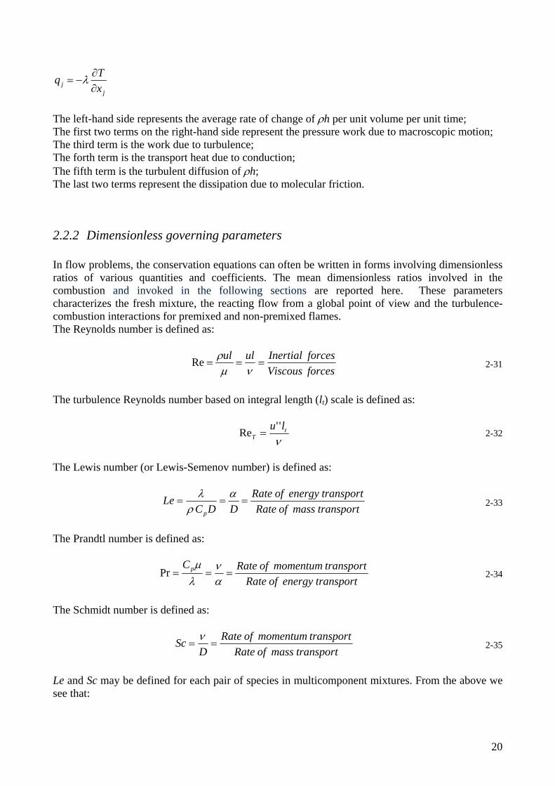
2.2.2 Dimensionless governing parameters In flow problems, the conservation equations can often be written in forms involving dimensionless ratios of various quantities and coefficients. The mean dimensionless ratios involved in the combustion and invoked in the following sections are reported here. These parameters characterizes the fresh mixture, the reacting flow from a global point of view and the turbulence-combustion interactions for premixed and non-premixed flames. The Reynolds number is defined as:

forcesViscousforcesInertialulul

===νμ

ρRe 2-31

The turbulence Reynolds number based on integral length (lt) scale is defined as:

νt

Tlu ''Re = 2-32

The Lewis number (or Lewis-Semenov number) is defined as:

transportmassofRatetransportenergyofRate

DDCLe

p

===α

ρλ 2-33

The Prandtl number is defined as:

transportenergyofRatetransportmomentumofRateCp ===

αν

λμ

Pr 2-34

The Schmidt number is defined as:

transportmassofRatetransportmomentumofRate

DSc ==

ν 2-35

Le and Sc may be defined for each pair of species in multicomponent mixtures. From the above we see that:

20

PrScLe = 2-36

In the following the Le number is approximately assumed 1(where not differently specified). An important parameter in combustion is the Damköhler number. This parameter appears in the description of many combustion problems and is quite important in understanding turbulent premixed flames (see following section). It is defined by:

( ) ( )LL

tt

c

tm

c

t

SlullDa

/''/

δττ

ττ

=== 2-37

It is defined for the largest eddies and corresponds to the ratio of the integral time scale (τt

turbulence time, characteristic flow time) to the chemical timescale (τc flame time). The subscript m stands for mechanical. δL is the laminar flame thickness, SL the laminar flame velocity and u’ the velocity fluctuations. From the definition, the Da can also represent the product of the length scale ratio and the reciprocal of a relative turbulence intensity. Thus, once fixed the length-scale ratio, the Da falls as turbulence intensity increases. The Karlovitz number is defined as:

( ) ( )

223

21

''1⎟⎟⎠

⎞⎜⎜⎝

⎛=⎟⎟

⎠

⎞⎜⎜⎝

⎛⎟⎟⎠

⎞⎜⎜⎝

⎛===

−

K

L

LL

t

Km

c

Ka lS

ulllDa

K δδτ

τ 2-38

It corresponds to the smallest eddies (Kolmogorov) and is the ratio of the chemical time scale to the Kolmogorov time.

2.2.3 Basic flame types In combustion processes, fuel and oxidizer are mixed and burned. There are several combustion categories based upon whether the fuel and oxidizer is mixed first and burned later (premixed) or whether combustion and mixing occur simultaneously (non premixed). Each of this categories can be further subdivided based on whether the fluid flow is laminar or turbulent. Next figure shows examples of combustion systems that belong to each of these categories, which will be discussed in the following sections.

21

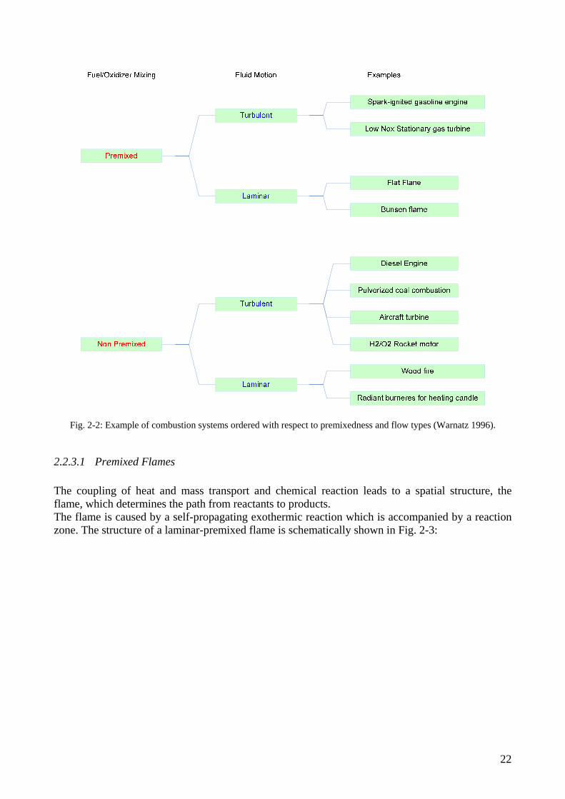
Fig. 2-2: Example of combustion systems ordered with respect to premixedness and flow types (Warnatz 1996).

2.2.3.1 Premixed Flames The coupling of heat and mass transport and chemical reaction leads to a spatial structure, the flame, which determines the path from reactants to products. The flame is caused by a self-propagating exothermic reaction which is accompanied by a reaction zone. The structure of a laminar-premixed flame is schematically shown in Fig. 2-3:

22

Fig. 2-3: Schematic representation of premixed flames structure.

Premixed flame structure can be divided into four zones: unburned zone (cold reactants zone), preheat zone, reaction zone and burned gas zone (products zone). The unburned mixture of fuel and oxidizer is delivered to the preheat zone at prefixed conditions, where the mixture is warmed by upstream heat transfer from the reaction zone. In the reaction zone, the fuel is rapidly consumed and the bulk of chemical energy is released. The thickness of the flame front depends on pressure and on initial temperature and equivalence ratio. This thin flame front implies steep species and temperature gradients, which provide the driving forces for the flame to be self-sustaining. In the reaction zone, temperature is high enough for creating a large radical pool. Finally, in the burned zone, radicals recombine, and both temperature and major species concentrations approach their equilibrium values. However, the concentrations of minor species in this region can deviate substantially from their equilibrium values. The velocity with which a flame front propagates with respect to the unburned fuel-oxidizer mixture is called the laminar burning velocity, SL, and is strongly dependent upon fuel and oxidizer type, equivalence ratio and temperature of unburned fuel-oxidizer mixture. Considering a premixed flammable mixture in a long tube, open at both ends, ignited from one end. A combustion wave will travel down the tube starting from the ignition point. The characteristic burning velocity depends upon the fuel. For most hydrocarbon-air stoichiometric mixtures this velocity is about 0.4 to 0.6 m/s, for hydrogen-air mixures this velocity is several meters per second. The velocity of this wave is controlled by the diffusion of heat and active radicals. Indicating the unburned fuel-oxidizer mixture velocity with v, the speed of the flame front vfr is v-SL. From the last relation three possible idealized situations may occur, depending on the relation between v and SL. First, if v>SL the flame will move away from the burner, i.e., the flame will blow off. If v=SL, the flame will keep its position relative to the burner surface, and be “aerodynamically stabilized”. In this case, neglecting possible radiative losses from the flame to the surroundings, the enthalpy in the fuel is solely manifest in the temperature of the burned gases, and the flame is referred to as an “adiabatic” or “free” flame. The temperature corresponding to an adiabatic flame is the maximum flame temperature that can be achieved for a given fuel-oxidizer composition. If v<SL, the flame will move towards the burner and will attempt to enter the burner (flash back). Since the pores of the idealized burner are assumed to prevent the flame from entering the burner, the flame will

23

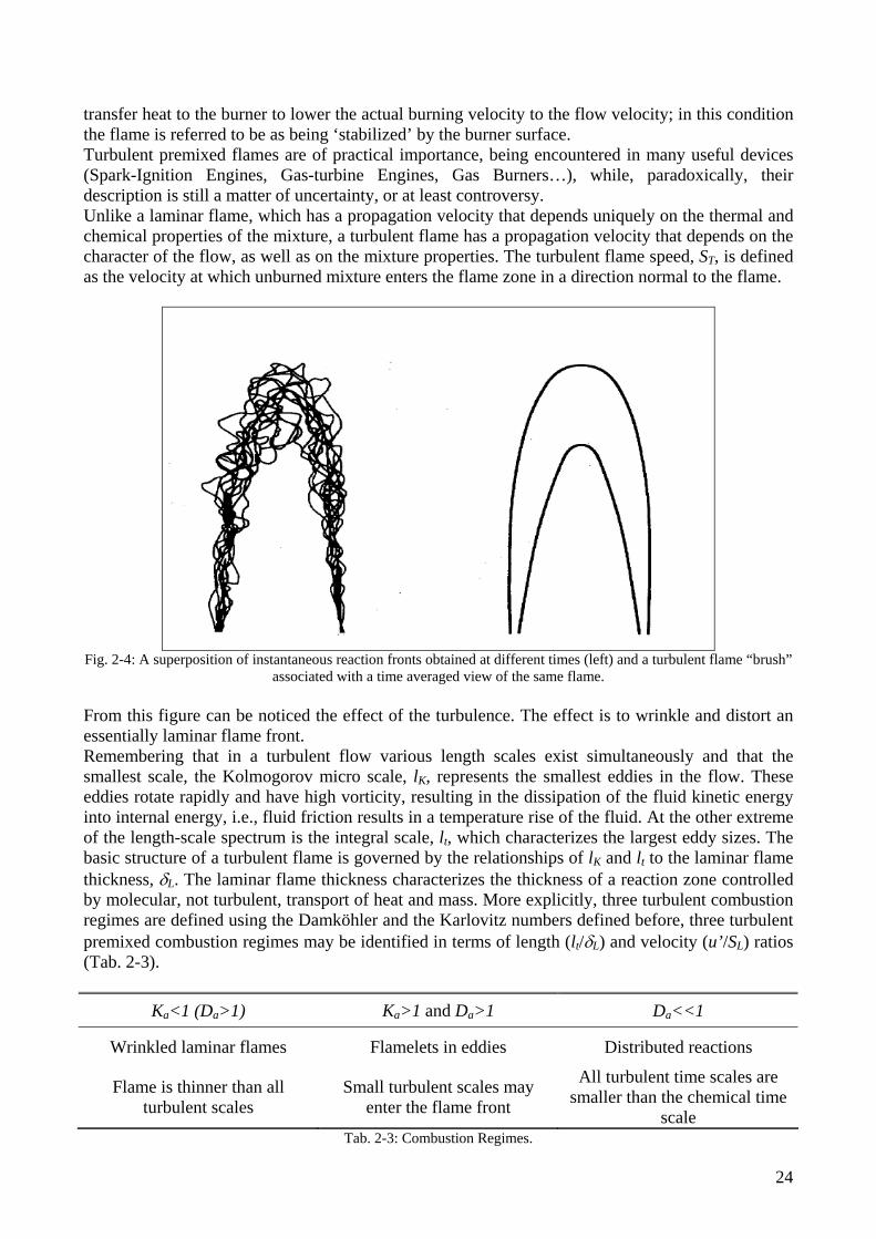
transfer heat to the burner to lower the actual burning velocity to the flow velocity; in this condition the flame is referred to be as being ‘stabilized’ by the burner surface. Turbulent premixed flames are of practical importance, being encountered in many useful devices (Spark-Ignition Engines, Gas-turbine Engines, Gas Burners…), while, paradoxically, their description is still a matter of uncertainty, or at least controversy. Unlike a laminar flame, which has a propagation velocity that depends uniquely on the thermal and chemical properties of the mixture, a turbulent flame has a propagation velocity that depends on the character of the flow, as well as on the mixture properties. The turbulent flame speed, ST, is defined as the velocity at which unburned mixture enters the flame zone in a direction normal to the flame.

Fig. 2-4: A superposition of instantaneous reaction fronts obtained at different times (left) and a turbulent flame “brush”

associated with a time averaged view of the same flame. From this figure can be noticed the effect of the turbulence. The effect is to wrinkle and distort an essentially laminar flame front. Remembering that in a turbulent flow various length scales exist simultaneously and that the smallest scale, the Kolmogorov micro scale, lK, represents the smallest eddies in the flow. These eddies rotate rapidly and have high vorticity, resulting in the dissipation of the fluid kinetic energy into internal energy, i.e., fluid friction results in a temperature rise of the fluid. At the other extreme of the length-scale spectrum is the integral scale, lt, which characterizes the largest eddy sizes. The basic structure of a turbulent flame is governed by the relationships of lK and lt to the laminar flame thickness, δL. The laminar flame thickness characterizes the thickness of a reaction zone controlled by molecular, not turbulent, transport of heat and mass. More explicitly, three turbulent combustion regimes are defined using the Damköhler and the Karlovitz numbers defined before, three turbulent premixed combustion regimes may be identified in terms of length (lt/δL) and velocity (u’/SL) ratios (Tab. 2-3).

Ka<1 (Da>1) Ka>1 and Da>1 Da<<1

Wrinkled laminar flames Flamelets in eddies Distributed reactions

Flame is thinner than all turbulent scales

Small turbulent scales may enter the flame front

All turbulent time scales are smaller than the chemical time

scale Tab. 2-3: Combustion Regimes.

24

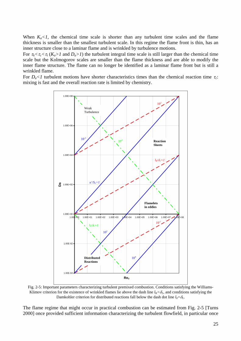
When Ka<1, the chemical time scale is shorter than any turbulent time scales and the flame thickness is smaller than the smallest turbulent scale. In this regime the flame front is thin, has an inner structure close to a laminar flame and is wrinkled by turbulence motions. For τk<τc<τt (Ka>1 and Da>1) the turbulent integral time scale is still larger than the chemical time scale but the Kolmogorov scales are smaller than the flame thickness and are able to modify the inner flame structure. The flame can no longer be identified as a laminar flame front but is still a wrinkled flame. For Da<1 turbulent motions have shorter characteristics times than the chemical reaction time τc: mixing is fast and the overall reaction rate is limited by chemistry.

1.00E-04

1.00E-02

1.00E+00

1.00E+02

1.00E+04

1.00E+06

1.00E+08

1.00E+00 1.00E+01 1.00E+02 1.00E+03 1.00E+04 1.00E+05 1.00E+06 1.00E+07 1.00E+08

ReT

Da

102

Weak Turbulence

10-2

104 Reaction Sheets

lK/δL=1

u’/SL=1

Flamelets in eddies

10-2

l0/δL=1

102

104Distributed Reactions

Fig. 2-5: Important parameters characterizing turbulent premixed combustion. Conditions satisfying the Williams-Klimov criterion for the existence of wrinkled flames lie above the dash line lK=δL, and conditions satisfying the

Damkohler criterion for distributed reactions fall below the dash dot line l0=δL. The flame regime that might occur in practical combustion can be estimated from Fig. 2-5 [Turns 2000] once provided sufficient information characterizing the turbulent flowfield, in particular once

25

identified five dimensionless parameters interrelated in the figure. The parameters are: lK/δL, l0/δL, ReT, Da and u’/SL. There are three separated regions on the graph of Da versus ReT corresponding to the three regimes defined before. The three regions are separated by the dash dot line l0/δL=1 and the dash line lK/δL=1. Above the dash line reactions take place in thin sheets, the wrinkled laminar-flame regime; below the dash dot line reactions will take place over a distributed region in space. The region between the lines is the flamelets in eddies regime.

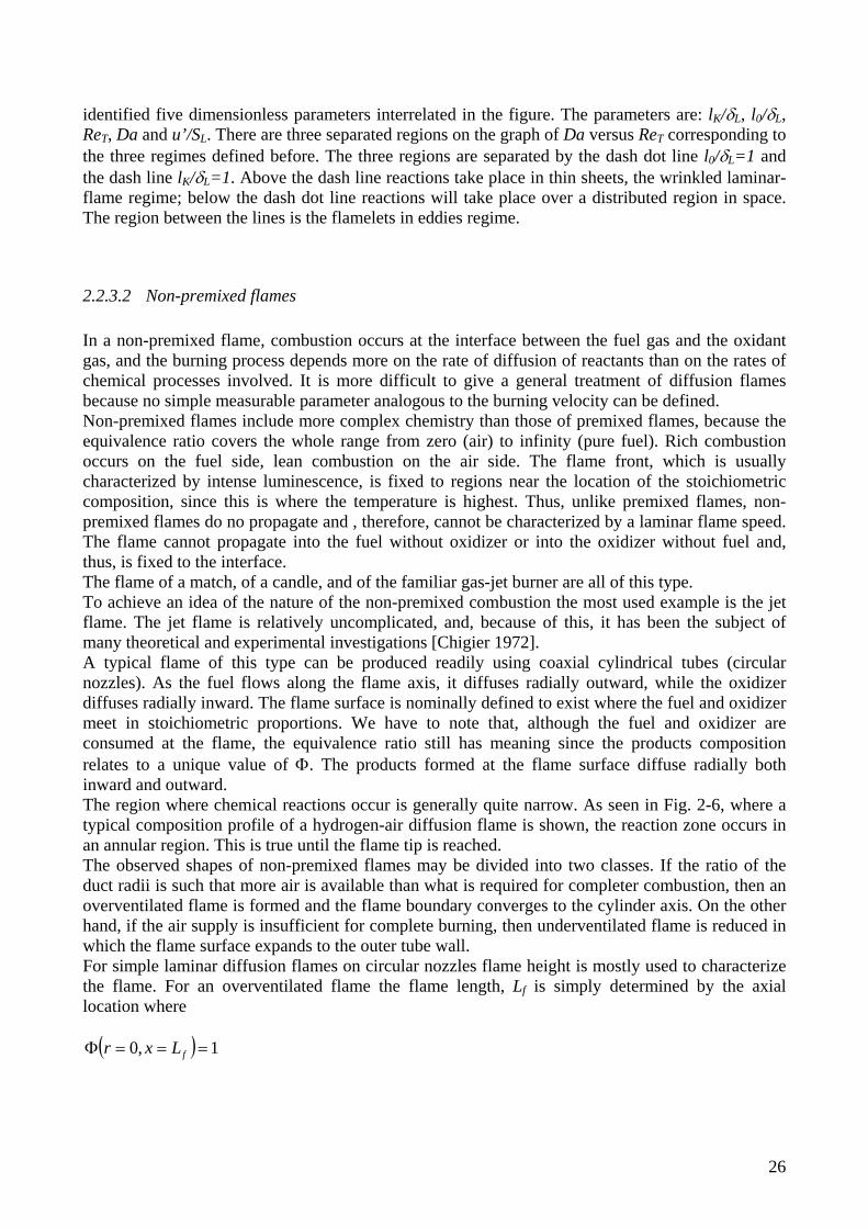
2.2.3.2 Non-premixed flames In a non-premixed flame, combustion occurs at the interface between the fuel gas and the oxidant gas, and the burning process depends more on the rate of diffusion of reactants than on the rates of chemical processes involved. It is more difficult to give a general treatment of diffusion flames because no simple measurable parameter analogous to the burning velocity can be defined. Non-premixed flames include more complex chemistry than those of premixed flames, because the equivalence ratio covers the whole range from zero (air) to infinity (pure fuel). Rich combustion occurs on the fuel side, lean combustion on the air side. The flame front, which is usually characterized by intense luminescence, is fixed to regions near the location of the stoichiometric composition, since this is where the temperature is highest. Thus, unlike premixed flames, non-premixed flames do no propagate and , therefore, cannot be characterized by a laminar flame speed. The flame cannot propagate into the fuel without oxidizer or into the oxidizer without fuel and, thus, is fixed to the interface. The flame of a match, of a candle, and of the familiar gas-jet burner are all of this type. To achieve an idea of the nature of the non-premixed combustion the most used example is the jet flame. The jet flame is relatively uncomplicated, and, because of this, it has been the subject of many theoretical and experimental investigations [Chigier 1972]. A typical flame of this type can be produced readily using coaxial cylindrical tubes (circular nozzles). As the fuel flows along the flame axis, it diffuses radially outward, while the oxidizer diffuses radially inward. The flame surface is nominally defined to exist where the fuel and oxidizer meet in stoichiometric proportions. We have to note that, although the fuel and oxidizer are consumed at the flame, the equivalence ratio still has meaning since the products composition relates to a unique value of Φ. The products formed at the flame surface diffuse radially both inward and outward. The region where chemical reactions occur is generally quite narrow. As seen in Fig. 2-6, where a typical composition profile of a hydrogen-air diffusion flame is shown, the reaction zone occurs in an annular region. This is true until the flame tip is reached. The observed shapes of non-premixed flames may be divided into two classes. If the ratio of the duct radii is such that more air is available than what is required for completer combustion, then an overventilated flame is formed and the flame boundary converges to the cylinder axis. On the other hand, if the air supply is insufficient for complete burning, then underventilated flame is reduced in which the flame surface expands to the outer tube wall. For simple laminar diffusion flames on circular nozzles flame height is mostly used to characterize the flame. For an overventilated flame the flame length, Lf is simply determined by the axial location where

( ) 1,0 ===Φ fLxr

26

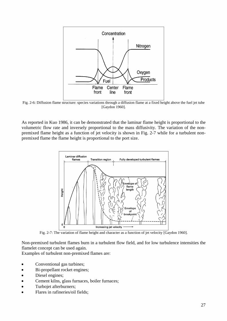
Fig. 2-6: Diffusion flame structure: species variations through a diffusion flame at a fixed height above the fuel jet tube

[Gaydon 1960]. As reported in Kuo 1986, it can be demonstrated that the laminar flame height is proportional to the volumetric flow rate and inversely proportional to the mass diffusivity. The variation of the non-premixed flame height as a function of jet velocity is shown in Fig. 2-7 while for a turbulent non-premixed flame the flame height is proportional to the port size.

Fig. 2-7: The variation of flame height and character as a function of jet velocity [Gaydon 1960].

Non-premixed turbulent flames burn in a turbulent flow field, and for low turbulence intensities the flamelet concept can be used again. Examples of turbulent non-premixed flames are: • Conventional gas turbines; • Bi-propellant rocket engines; • Diesel engines; • Cement kilns, glass furnaces, boiler furnaces; • Turbojet afterburners; • Flares in rafineries/oil fields;

27

• Most fires (like forest fires), pool flames; • Coal/wood combustion; For any particular application, some of the issues the designer is faced with are as follows (importance of each may change depending on the nature of the application): combustion intensity and efficiency, flame stability shape and size, heat transport and pollutant emissions. Because of the safety considerations mentioned above and the ease with which such flames can be controlled, non-premixed flames are mostly used in industrial furnaces and burners, the majority of practical combustion systems. With current concern for pollutant emissions, however, this advantage becomes something of a liability in that there is also less ability to control, or tailor, the combustion process for low emissions. Unless very sophisticated mixing are used, non premixed flames show a yellow luminescence (Fig. 2-8), caused by glowing soot particles, which are formed by fuel rich chemical reactions in the rich domain of the non-premixed flames; the non-premixed turbulent jet flames have brushy or fuzzy edges similar to premixed flames.

Fig. 2-8:Turbulent non-premixed flames.

As mentioned before, the height of the laminar flame depends on the flow rate. As the flow rate increases, turbulence begins to influence the flame height and a transitional regime can be seen. Over this transitional, the increasing turbulence levels with flowrate result in the fully turbulent flames being shorter than their laminar counterparts. Concerning flame stability, at sufficiently low flowrates, the base of a jet flame lies quite close to the burner tube outlet and is said to be attached. As the fuel flowrate is increased, holes begin to form in the flame sheet at the base of the flame, and with further increase in the flowrate, more and more holes form until there is no continuous flame close to the burner port (Liftoff). At sufficiently large flow rate, the flame blows out.

2.3 Chemical kinetics and reaction mechanisms Chemical kinetics is the part of chemical science dealing with the quantitative study of the rates of chemical reactions and of the factors upon which they depend. It also deals with the interpretation of the empirical kinetic laws in terms of reaction mechanisms. A reaction mechanism is a collection of elementary reactions necessary to describe an overall reaction. We remind to e.g. Kuo 1986, Glassman 1996, Peters 1993, Smoke 1991, Turns 2000 for more details.

28

Some of the essential features of chemical kinetics which occur frequently in this work will be reviewed in the following sections.

2.3.1 Rates of reactions All chemical reactions, whether hydrolysis or combustion, take place at a definite rate, depending on the conditions of the system. Some important conditions are concentrations of the chemical compounds, temperature, pressure, presence of a catalyst or inhibitor, and radiative effects. The rate of reaction may be expressed in terms of the concentration of any reactant as the rate of decrease of the concentration of that reactant (the rate of consumption of the reactant). It may also be expressed in terms of product concentration as the rate of increase of the product concentration. A conventional unit for reaction rate is moles/m3 sec. The rate law for an elementary reaction can be described by the equation:

...... FEDCBA k ++⎯→⎯+++ 2-39 Where A,B,C… denote the different species involved in the reaction. A rate law describes an empirical formulation of the reaction rate, i.e. the rate of formation or consumption of a species in a chemical reaction. The law of mass action, which is confirmed by numerous experimental observations, states that the rate of disappearance of a chemical species is proportional to the products of the concentrations of the reacting chemical species, each concentration being raised to a power equal to the corresponding stoichiometric coefficient. Looking at the consumption of species A, the reaction rate can be expressed according to

[ ] [ ] [ ] [ ] ....cba CBAkdtAd

⋅−= 2-40

Where a,b,c.. are reaction orders with respects to the species A,B,C… and k is the rate coefficient of the reaction (or specific reaction rate constant). The sum of all exponents is the overall reaction order. For the reverse reaction (characterized here by the subscript r) one obtains the rate law for the production of A:

[ ] [ ] [ ] [ ] ....fedr FEDk

dtAd

⋅= 2-41

Since mechanisms may involve many elementary steps and many species, the compact notation can be used to represent both the mechanism and the individual species production rates. For the mechanism, one can write:

∑∑==

⇔N

jjji

N

jjji AA

11''' νν for i=1,2,…,L. 2-42

Where ν’ji and ν’’ji are the stoichiometric coefficients on the reactants and products side of the equation, respectively, for the jth species and ith reaction. Aj is the arbitrary specification of all chemical species and N the total number of compounds involved.

29

The following three relations compactly express the net production rate of each species in a multistep mechanism:

[ ]∑

=

==L

iijij

j qdtAd

1νω& for j=1,2,…,N. 2-43

Where

( )jijiji ''' ννν −= 2-44

And

[ ] [ ]∏∏==

−=N

jjri

N

jjfii

jiji AkAkq1

''

1

' νν 2-45

The last equation defines the rate of progress variable, qi, for the ith elementary reaction. The specific reaction-rate constant, for a given reaction, is independent of the concentrations [Aj] and depends only on the temperature. In general, k is expressed as:

⎟⎟⎠

⎞⎜⎜⎝

⎛−=

TREATk

u

an exp 2-46

Where ATn represents the collision frequency and the exponential term is the Boltzmann factor, specifying the fraction of collisions that have an energy greater than the activation energy Ea. The values of B, n and Ea are based on the nature of the elementary reaction. For given chemical changes, these parameters are neither functions of the concentrations nor of temperature.

2.3.2 Hydrogen Chemical Mechanism The H2-O2 reaction mechanism has been extensively studied over the years and has already got widespread application such as in high energy rocket engines. More recently it has become extremely evident that combustion of hydrogen with air will continue to receive increasing application primarily because of the non-polluting characteristics of this combustion process. In this contest it is essential to discuss the hydrogen oxygen combustion reactive mechanism. It has been observed that under ambient conditions of temperature, hydrogen and oxygen do not enter into any direct reaction between them in absence of a catalyst. It is further seen if a mixture of hydrogen and oxygen gets exposed to light oxygen gets activated usually by way of dissociation. In the presence of the sensitizers of Cl, N2O and NH3, a set of secondary reactions take place and form H atoms. These H atoms enter into a reaction with the activated oxygen thus forming H2O. Relying heavily on Glassman 1996, the oxidation of hydrogen is as follows. The initiation reactions are

MHHMH ++⇒+2 (very high temperature) HHOOH +⇒+ 222 (other temperatures).

30

Chain-reaction steps involving O, H and OH radicals are

OHOOH +⇒+ 2 OHHHO +⇒+ 2

HOHOHH +⇒+ 22 OHOHOHO +⇒+ 2 .

Chain-terminating steps involving O, H and OH radicals are the three-body recombination reactions:

MHMHH +⇒++ 2 MOMOO +⇒++ 2

MOHMOH +⇒++ MOHMOHH +⇒++ 2 .

To complete the mechanism, the reactions involving HO2, the hydroperoxy radical, and H2O2, hydrogen peroxide need to be included. When

MHOMOH +⇒++ 22 Becomes active, then the following reactions come into play:

OHOHHHO +⇒+2 OOHHHO +⇒+ 22

OHOOHO +⇒+ 22 And

22222 OOHHOHO +⇒+ HOHHHO +⇒+ 2222

With

2222 HOOHOHOH +⇒+ OHOHHOH +⇒+ 222

2222 HHOHOH +⇒+ MOHOHMOH ++⇒+22

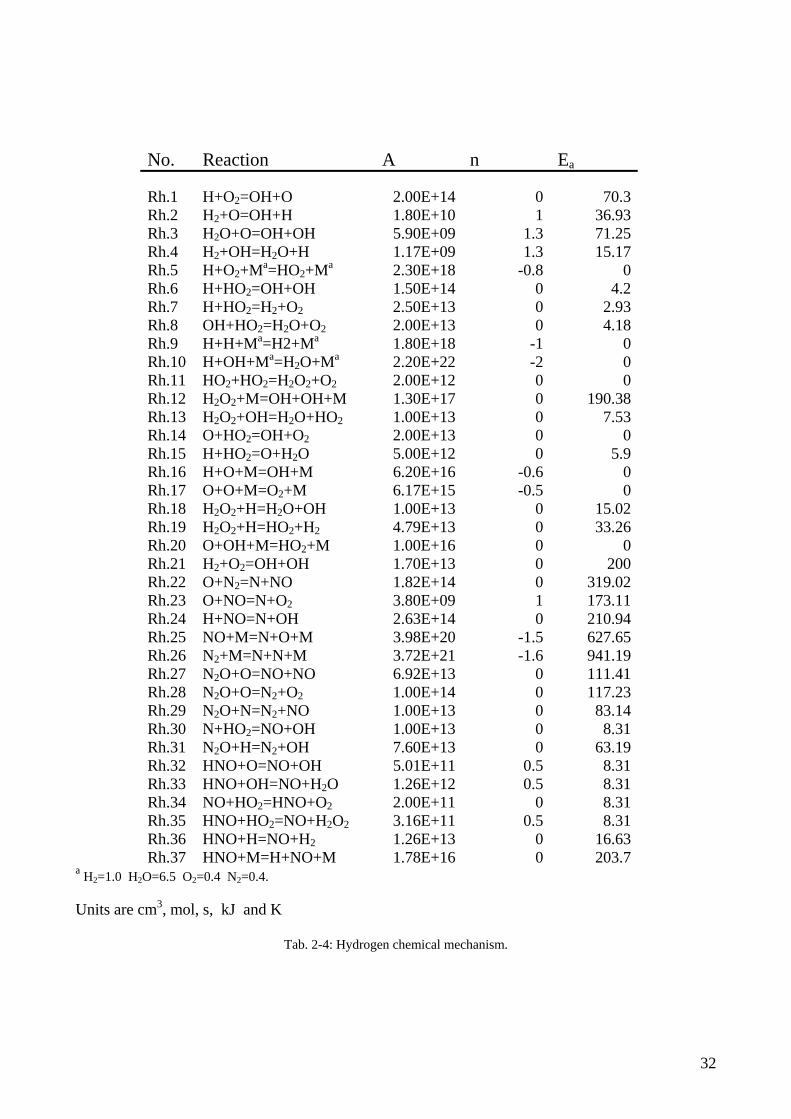
Depending upon the temperature, pressure and extent of reaction, the reverse reactions of all of above can be important; therefore in modelling H2-O2 system as many as 40 reactions can be taken into account involving eight species: H2, O2, H2O, OH, O, H, HO2 and H2O2. The H2 chemical mechanism used in the simulations is reported in the following table.

31

No. Reaction A n Ea Rh.1 H+O2=OH+O 2.00E+14 0 70.3 Rh.2 H2+O=OH+H 1.80E+10 1 36.93 Rh.3 H2O+O=OH+OH 5.90E+09 1.3 71.25 Rh.4 H2+OH=H2O+H 1.17E+09 1.3 15.17 Rh.5 H+O2+Ma=HO2+Ma 2.30E+18 -0.8 0 Rh.6 H+HO2=OH+OH 1.50E+14 0 4.2 Rh.7 H+HO2=H2+O2 2.50E+13 0 2.93 Rh.8 OH+HO2=H2O+O2 2.00E+13 0 4.18 Rh.9 H+H+Ma=H2+Ma 1.80E+18 -1 0 Rh.10 H+OH+Ma=H2O+Ma 2.20E+22 -2 0 Rh.11 HO2+HO2=H2O2+O2 2.00E+12 0 0 Rh.12 H2O2+M=OH+OH+M 1.30E+17 0 190.38 Rh.13 H2O2+OH=H2O+HO2 1.00E+13 0 7.53 Rh.14 O+HO2=OH+O2 2.00E+13 0 0 Rh.15 H+HO2=O+H2O 5.00E+12 0 5.9 Rh.16 H+O+M=OH+M 6.20E+16 -0.6 0 Rh.17 O+O+M=O2+M 6.17E+15 -0.5 0 Rh.18 H2O2+H=H2O+OH 1.00E+13 0 15.02 Rh.19 H2O2+H=HO2+H2 4.79E+13 0 33.26 Rh.20 O+OH+M=HO2+M 1.00E+16 0 0 Rh.21 H2+O2=OH+OH 1.70E+13 0 200 Rh.22 O+N2=N+NO 1.82E+14 0 319.02 Rh.23 O+NO=N+O2 3.80E+09 1 173.11 Rh.24 H+NO=N+OH 2.63E+14 0 210.94 Rh.25 NO+M=N+O+M 3.98E+20 -1.5 627.65 Rh.26 N2+M=N+N+M 3.72E+21 -1.6 941.19 Rh.27 N2O+O=NO+NO 6.92E+13 0 111.41 Rh.28 N2O+O=N2+O2 1.00E+14 0 117.23 Rh.29 N2O+N=N2+NO 1.00E+13 0 83.14 Rh.30 N+HO2=NO+OH 1.00E+13 0 8.31 Rh.31 N2O+H=N2+OH 7.60E+13 0 63.19 Rh.32 HNO+O=NO+OH 5.01E+11 0.5 8.31 Rh.33 HNO+OH=NO+H2O 1.26E+12 0.5 8.31 Rh.34 NO+HO2=HNO+O2 2.00E+11 0 8.31 Rh.35 HNO+HO2=NO+H2O2 3.16E+11 0.5 8.31 Rh.36 HNO+H=NO+H2 1.26E+13 0 16.63 Rh.37 HNO+M=H+NO+M 1.78E+16 0 203.7

a H2=1.0 H2O=6.5 O2=0.4 N2=0.4. Units are cm3, mol, s, kJ and K

Tab. 2-4: Hydrogen chemical mechanism.

32

2.3.3 Oxides of nitrogen formation Nitric oxide is an important minor species in combustion because of its contribution to air pollution. The detailed nitrogen chemistry involved in the combustion of methane is reported in the GRIMECH mechanism [GRI-Mech 3.0]. In the combustion of fuels that contain no nitrogen, nitric oxide is formed by three chemical mechanisms or routes that involve nitrogen from the air: the thermal or Zeldovich mechanism, the Fenimore or prompt mechanism and the N2O intermediate mechanism. There is growing evidence for the possibility of a fourth route involving NNH. The thermal mechanism dominates in high-temperature combustion over a fairly wide range of equivalence ratios, while the Fenimore mechanism is particularly important in rich combustion. It appears that the N2O-intermediate mechanism plays an important role in the production of NO in very lean, low-temperature combustion processes. Recent studies show the relative contributions of the three mechanisms in premixed and diffusion flames. The thermal or Zeldovich mechanism consists of two chain reactions:

NNONO +⇔+ 2 ONOON +⇔+ 2

Which can be extended by adding the reaction

HNOOHN +⇔+ This three-reaction set is referred as the extended Zeldovich mechanism. In general, this mechanism is coupled to the fuel combustion chemistry through the O2, O, and OH species; however, in process where the fuel combustion is complete before NO formation becomes significant, the two processes can be uncoupled. In this case, if the relevant time scales are sufficiently long, one can assume that the N2, O2, O, and OH concentrations are at their equilibrium values and N atoms are in steady state. These assumptions greatly simplify the problem of calculating the NO formation. If we make the additional assumption that the NO concentrations are much less than their equilibrium values, the reverse reactions can be neglected. This yields the following rather simple rate expression:

[ ] [ ] [ ]eqeqfN NOkdtNOd

21.2= 2-47

Within flame zones proper and in short-time-scale, postflame processes, the equilibrium assumption is not valid. Superequilibrium concentrations of O atoms, up to several orders of magnitude greater than equilibrium, greatly increase NO formation rates. This superequilibrium O (and OH) atom contribution to NO production rates is sometimes classified as part of the so-called prompt-NO mechanism. The activation energy for the first NO reaction is relatively large; thus, this reaction has a very strong temperature dependence. As a rule-of-thumb, the thermal mechanism is usually unimportant at temperatures below 1800 K. Compared with the time scales of fuel oxidation processes, NO is formed rather slowly by the thermal mechanism; thus, thermal NO is generally considered to be formed in the postflame gases. The N2O-intermediate mechanism is important in fuel-lean (F<0.8), low temperature conditions. The three steps of this mechanism are

33

MONMNO +⇔++ 22 NHNOONH +⇔+ 2 NONOONO +⇔+ 2

This Mechanism becomes important in NO control strategies that involve lean premixed combustion, which are currently being explored by gas-turbine manufacturers. The Fenimore mechanism is intimately linked to the combustion chemistry of hydrocarbons [Lefebvre 1983]. Fenimore discovered that some NO was rapidly produced in the flame zone of laminar premixed flames long before there would be time to form NO by the thermal mechanism, and he gave this rapidly formed NO the appellation prompt NO. The general scheme of the Fenimore mechanism is that hydrocarbon radicals react with molecular nitrogen to form amines or cyano compounds. The amines and cyano compounds are then converted to intermediate compounds that ultimately form NO. In the atmosphere, nitric oxide ultimately oxidizes to form nitrogen dioxide, which is important to the production of acid rain and photochemical smog. Many combustion processes, however, emit significant fractions of their total oxides of nitrogen as NO2. the elementary reactions responsible for forming NO2 prior to exhausting of the combustion products into the atmosphere are the following:

OHNOHONO +⇔+ 22 (formation) OHNOHNO +⇔+2 (destruction)

22 ONOONO +⇔+ (destruction) Where the HO2 radical is formed by the three-body reaction:

MHOMOH +⇔++ 22 The HO2 radicals are formed in relatively low-temperature regions; hence, NO2 formation occurs when NO molecules from high temperature regions diffuse or are transported by fluid mixing into HO2 rich regions. The NO2 destruction reactions are active at high temperatures, thus preventing the formation of NO2 in high-temperature zones.

2.4 Mild Combustion One of the major advantages into the application of the TVC combustors is the possibility to achieve mild combustion that is one of the promising techniques proposed to control pollutant emissions from combustion plants. It is characterized by high pre-heating of combustion air and massive recycle of burned gas before reaction. Real-size burners achieve flameless conditions by feeding the combustion air and the fuel through separated or coflowing high velocity jets into the combustion chamber. The air jets entrain a large amount of burned gases from the combustion chamber before reacting with the fuel. Consequently oxygen concentration in combustion air is lower than in traditional flames, while turbulence is higher. Chemical reactions occur at lower rates (compared with mixing ones) and are less limited by mass diffusion. Consequently, the combustion region is no longer concentrated close to the flame front but is extended over the whole combustion chamber, resulting in a volumetric rather than superficial combustion and in the complete disappearance of the flame, hence the name flameless. As a result, mild oxidation can easily control thermal gradients by avoiding the formation of hot

34

spots in the furnace and by enabling reduction of thermal NOx production without compromising combustion efficiency. Another peculiar characteristic is the reduction of combustion noise, which is set to values similar to those generated by a non-reacting jet [Wünning 1997].

35

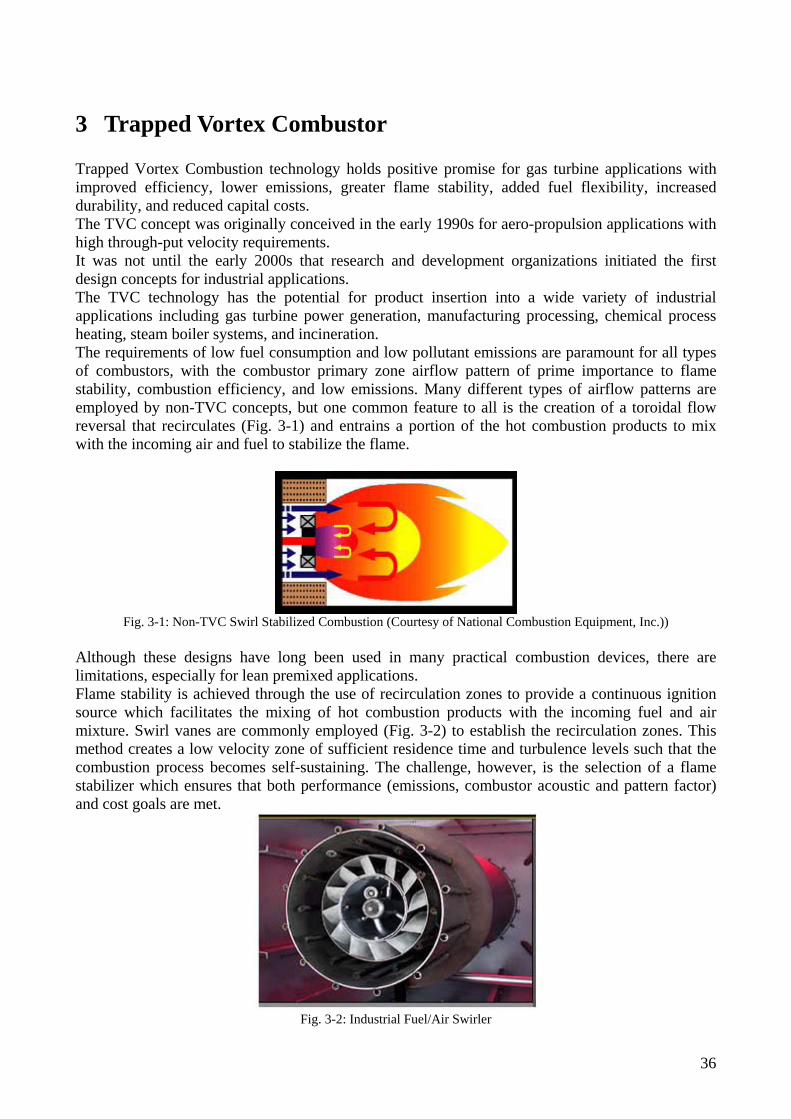
3 Trapped Vortex Combustor Trapped Vortex Combustion technology holds positive promise for gas turbine applications with improved efficiency, lower emissions, greater flame stability, added fuel flexibility, increased durability, and reduced capital costs. The TVC concept was originally conceived in the early 1990s for aero-propulsion applications with high through-put velocity requirements. It was not until the early 2000s that research and development organizations initiated the first design concepts for industrial applications. The TVC technology has the potential for product insertion into a wide variety of industrial applications including gas turbine power generation, manufacturing processing, chemical process heating, steam boiler systems, and incineration. The requirements of low fuel consumption and low pollutant emissions are paramount for all types of combustors, with the combustor primary zone airflow pattern of prime importance to flame stability, combustion efficiency, and low emissions. Many different types of airflow patterns are employed by non-TVC concepts, but one common feature to all is the creation of a toroidal flow reversal that recirculates (Fig. 3-1) and entrains a portion of the hot combustion products to mix with the incoming air and fuel to stabilize the flame.

Fig. 3-1: Non-TVC Swirl Stabilized Combustion (Courtesy of National Combustion Equipment, Inc.))

Although these designs have long been used in many practical combustion devices, there are limitations, especially for lean premixed applications. Flame stability is achieved through the use of recirculation zones to provide a continuous ignition source which facilitates the mixing of hot combustion products with the incoming fuel and air mixture. Swirl vanes are commonly employed (Fig. 3-2) to establish the recirculation zones. This method creates a low velocity zone of sufficient residence time and turbulence levels such that the combustion process becomes self-sustaining. The challenge, however, is the selection of a flame stabilizer which ensures that both performance (emissions, combustor acoustic and pattern factor) and cost goals are met.

Fig. 3-2: Industrial Fuel/Air Swirler

36

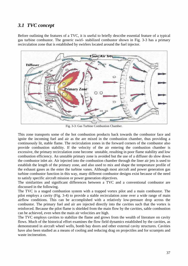
3.1 TVC concept Before outlining the features of a TVC, it is useful to briefly describe essential feature of a typical gas turbine combustor. The generic swirl- stabilized combustor shown in Fig. 3-3 has a primary recirculation zone that is established by swirlers located around the fuel injector.

Liner Air Jets

Diffuser

Primary Zone

Fig. 3-3: Gas Turbine Combustion Chamber. This zone transports some of the hot combustion products back towards the combustor face and ignite the incoming fuel and air as the are mixed in the combustion chamber, thus providing a continuously lit, stable flame. The recirculation zones in the forward corners of the combustor also provide combustion stability. If the velocity of the air entering the combustion chamber is excessive, the primary recirculation zone become unstable, resulting in poor flame stability and low combustion efficiency. An unstable primary zone is avoided but the use of a diffuser do slow down the combustor inlet air. Air injected into the combustion chamber through the liner air jets is used to establish the length of the primary zone, and also used to mix and shape the temperature profile of the exhaust gases as the enter the turbine vanes. Although most aircraft and power generation gas turbine combustor function in this way, many different combustor designs exist because of the need to satisfy specific aircraft mission or power generation objectives. The similarities and significant differences between a TVC and a conventional combustor are discussed in the following. The TVC is a staged combustion system with a trapped vortex pilot and a main combustor. The pilot employs a cavity (Fig. 3-4) to provide a stable recirculation zone over a wide range of main airflow conditions. This can be accomplished with a relatively low-pressure drop across the combustor. The primary fuel and air are injected directly into the cavities such that the vortex is reinforced. Because the pilot flame is shielded from the main flow by the cavities, sable combustion can be achieved, even when the main air velocities are high. The TVC employs cavities to stabilize the flame and grows from the wealth of literature on cavity flows. Much of the historical effort examines the flow field dynamics established by the cavities, as demonstrated in aircraft wheel wells, bomb bay doors and other external cavity structures. Cavities have also been studied as a means of cooling and reducing drag on projectiles and for scramjets and waste incineration.

37

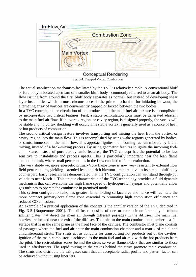
Fig. 3-4: Trapped Vortex Combustion.

The actual stabilization mechanism facilitated by the TVC is relatively simple. A conventional bluff or fore body is located upstream of a smaller bluff body - commonly referred to as an aft body. The flow issuing from around the first bluff body separates as normal, but instead of developing shear layer instabilities which in most circumstances is the prime mechanism for initiating blowout, the alternating array of vortices are conveniently trapped or locked between the two bodies. In a TVC concept, the re-circulation of hot products into the main fuel-air mixture is accomplished by incorporating two critical features. First, a stable recirculation zone must be generated adjacent to the main fuel-air flow. If the vortex region, or cavity region, is designed properly, the vortex will be stable and no vortex shedding will occur. This stable vortex is generally used as a source of heat, or hot products of combustion. The second critical design feature involves transporting and mixing the heat from the vortex, or cavity, region into the main flow. This is accomplished by using wake regions generated by bodies, or struts, immersed in the main flow. This approach ignites the incoming fuel-air mixture by lateral mixing, instead of a back-mixing process. By using geometric features to ignite the incoming fuel-air mixture, instead of pure aerodynamic features, the TVC concept has the potential to be less sensitive to instabilities and process upsets. This is particularly important near the lean flame extinction limit, where small perturbations in the flow can lead to flame extinction. The very stable yet more energetic primary/core flame zone is now very resistant to external flow field perturbations, yielding extended lean and rich blowout limits relative to its simple bluff body counterpart. Early research has demonstrated that the TVC configuration can withstand through-put velocities near Mach 1. This unique characteristic of the TVC technology provides a fluid dynamic mechanism that can overcome the high flame speed of hydrogen-rich syngas and potentially allow gas turbines to operate the combustor in premixed mode. This system configuration also has greater flame holding surface area and hence will facilitate the more compact primary/core flame zone essential to promoting high combustion efficiency and reduced CO emissions. An example of a pratical application of the concept is the annular version of the TVC depicted in Fig. 3-5 [Roquemore 2001]. The diffuser consists of one or more circumferentially distribute splitter plates that direct the main air through different passages in the diffuser. The main fuel nozzles are located near the exit of the diffuser. The inlet to the main combustion chamber is a flat surface that is in the same plane as the front face of the cavities. The combustor inlet plane consists of passages where the fuel and air enter the main combustion chamber and a matrix of radial and circumferential struts. The struts act as conduits for transporting hot products out of the cavities. Ignition of the main combustor is achieved as the main fuel and air mix with the hot products from the pilot. The recirculation zones behind the struts serve as flameholders that are similar to those used in afterburners. The rapid mixing in the wakes behind the struts promote rapid combustion. The struts also distribute the exit gases such that an acceptable radial profile and pattern factor can be achieved without using liner jets.

38

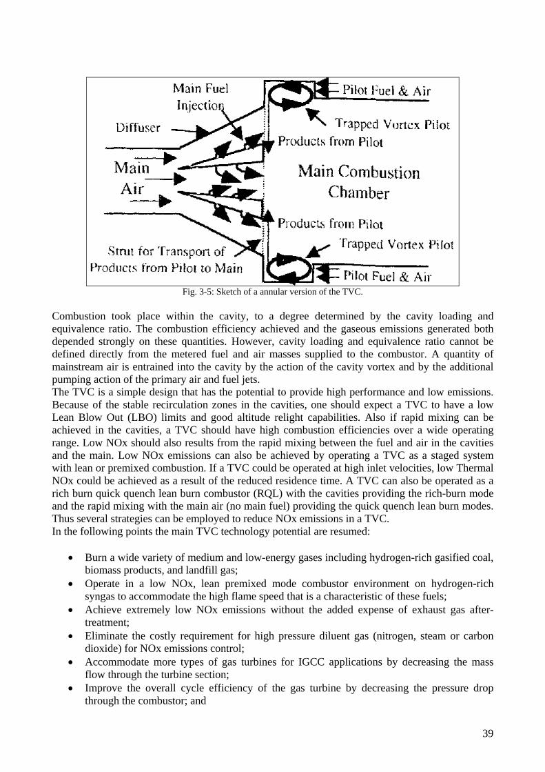
Fig. 3-5: Sketch of a annular version of the TVC.

Combustion took place within the cavity, to a degree determined by the cavity loading and equivalence ratio. The combustion efficiency achieved and the gaseous emissions generated both depended strongly on these quantities. However, cavity loading and equivalence ratio cannot be defined directly from the metered fuel and air masses supplied to the combustor. A quantity of mainstream air is entrained into the cavity by the action of the cavity vortex and by the additional pumping action of the primary air and fuel jets. The TVC is a simple design that has the potential to provide high performance and low emissions. Because of the stable recirculation zones in the cavities, one should expect a TVC to have a low Lean Blow Out (LBO) limits and good altitude relight capabilities. Also if rapid mixing can be achieved in the cavities, a TVC should have high combustion efficiencies over a wide operating range. Low NOx should also results from the rapid mixing between the fuel and air in the cavities and the main. Low NOx emissions can also be achieved by operating a TVC as a staged system with lean or premixed combustion. If a TVC could be operated at high inlet velocities, low Thermal NOx could be achieved as a result of the reduced residence time. A TVC can also be operated as a rich burn quick quench lean burn combustor (RQL) with the cavities providing the rich-burn mode and the rapid mixing with the main air (no main fuel) providing the quick quench lean burn modes. Thus several strategies can be employed to reduce NOx emissions in a TVC. In the following points the main TVC technology potential are resumed:

• Burn a wide variety of medium and low-energy gases including hydrogen-rich gasified coal, biomass products, and landfill gas;

• Operate in a low NOx, lean premixed mode combustor environment on hydrogen-rich syngas to accommodate the high flame speed that is a characteristic of these fuels;

• Achieve extremely low NOx emissions without the added expense of exhaust gas after-treatment;

• Eliminate the costly requirement for high pressure diluent gas (nitrogen, steam or carbon dioxide) for NOx emissions control;

• Accommodate more types of gas turbines for IGCC applications by decreasing the mass flow through the turbine section;

• Improve the overall cycle efficiency of the gas turbine by decreasing the pressure drop through the combustor; and

39

• Extend the lean blowout limit offering greater turndown, (load following), with improved combustion and process stability.

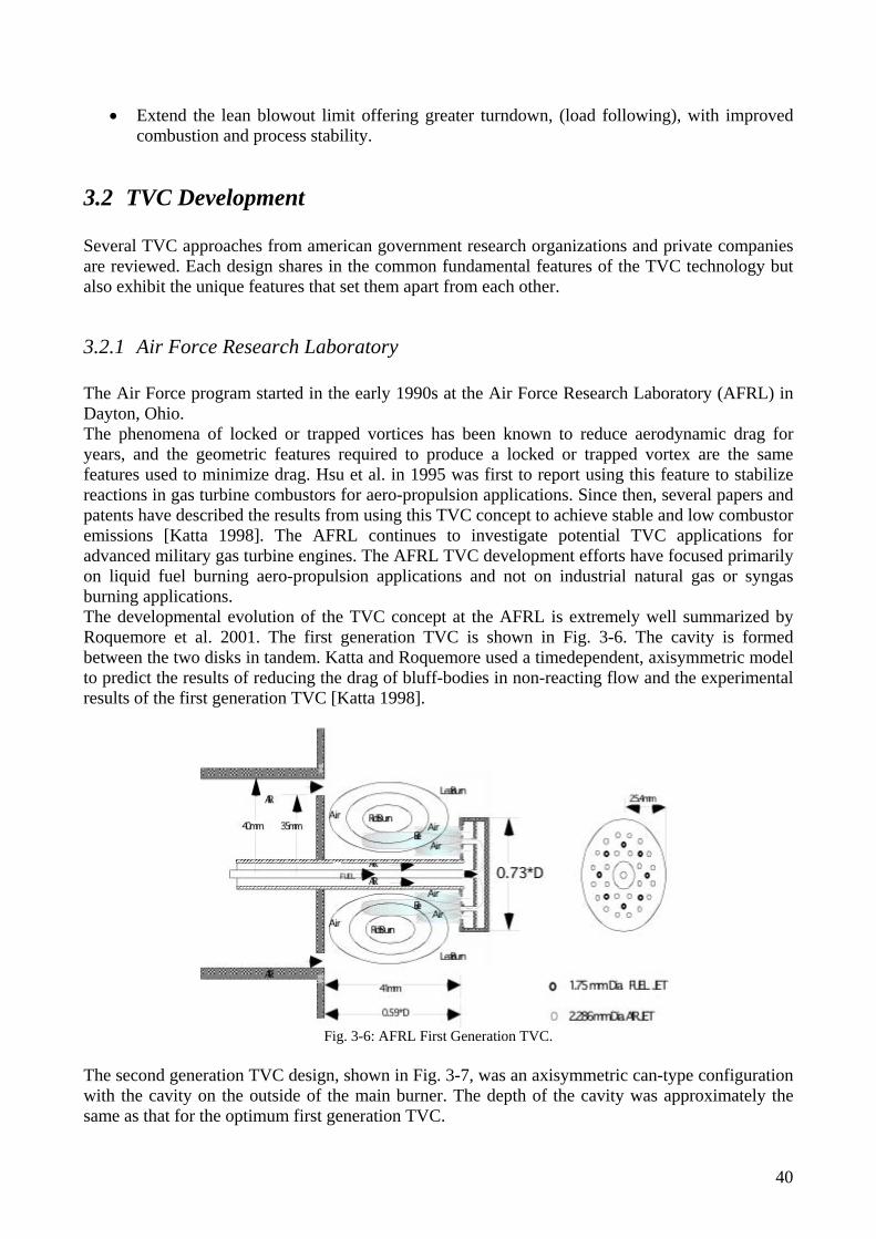
3.2 TVC Development Several TVC approaches from american government research organizations and private companies are reviewed. Each design shares in the common fundamental features of the TVC technology but also exhibit the unique features that set them apart from each other.

3.2.1 Air Force Research Laboratory The Air Force program started in the early 1990s at the Air Force Research Laboratory (AFRL) in Dayton, Ohio. The phenomena of locked or trapped vortices has been known to reduce aerodynamic drag for years, and the geometric features required to produce a locked or trapped vortex are the same features used to minimize drag. Hsu et al. in 1995 was first to report using this feature to stabilize reactions in gas turbine combustors for aero-propulsion applications. Since then, several papers and patents have described the results from using this TVC concept to achieve stable and low combustor emissions [Katta 1998]. The AFRL continues to investigate potential TVC applications for advanced military gas turbine engines. The AFRL TVC development efforts have focused primarily on liquid fuel burning aero-propulsion applications and not on industrial natural gas or syngas burning applications. The developmental evolution of the TVC concept at the AFRL is extremely well summarized by Roquemore et al. 2001. The first generation TVC is shown in Fig. 3-6. The cavity is formed between the two disks in tandem. Katta and Roquemore used a timedependent, axisymmetric model to predict the results of reducing the drag of bluff-bodies in non-reacting flow and the experimental results of the first generation TVC [Katta 1998].

Fig. 3-6: AFRL First Generation TVC.

The second generation TVC design, shown in Fig. 3-7, was an axisymmetric can-type configuration with the cavity on the outside of the main burner. The depth of the cavity was approximately the same as that for the optimum first generation TVC.

40

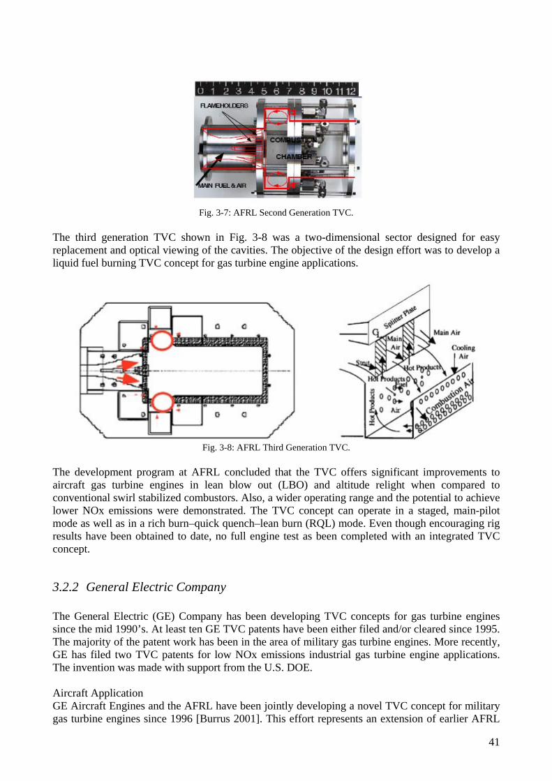
Fig. 3-7: AFRL Second Generation TVC.

The third generation TVC shown in Fig. 3-8 was a two-dimensional sector designed for easy replacement and optical viewing of the cavities. The objective of the design effort was to develop a liquid fuel burning TVC concept for gas turbine engine applications.

Fig. 3-8: AFRL Third Generation TVC.

The development program at AFRL concluded that the TVC offers significant improvements to aircraft gas turbine engines in lean blow out (LBO) and altitude relight when compared to conventional swirl stabilized combustors. Also, a wider operating range and the potential to achieve lower NOx emissions were demonstrated. The TVC concept can operate in a staged, main-pilot mode as well as in a rich burn–quick quench–lean burn (RQL) mode. Even though encouraging rig results have been obtained to date, no full engine test as been completed with an integrated TVC concept.

3.2.2 General Electric Company The General Electric (GE) Company has been developing TVC concepts for gas turbine engines since the mid 1990’s. At least ten GE TVC patents have been either filed and/or cleared since 1995. The majority of the patent work has been in the area of military gas turbine engines. More recently, GE has filed two TVC patents for low NOx emissions industrial gas turbine engine applications. The invention was made with support from the U.S. DOE. Aircraft Application GE Aircraft Engines and the AFRL have been jointly developing a novel TVC concept for military gas turbine engines since 1996 [Burrus 2001]. This effort represents an extension of earlier AFRL

41

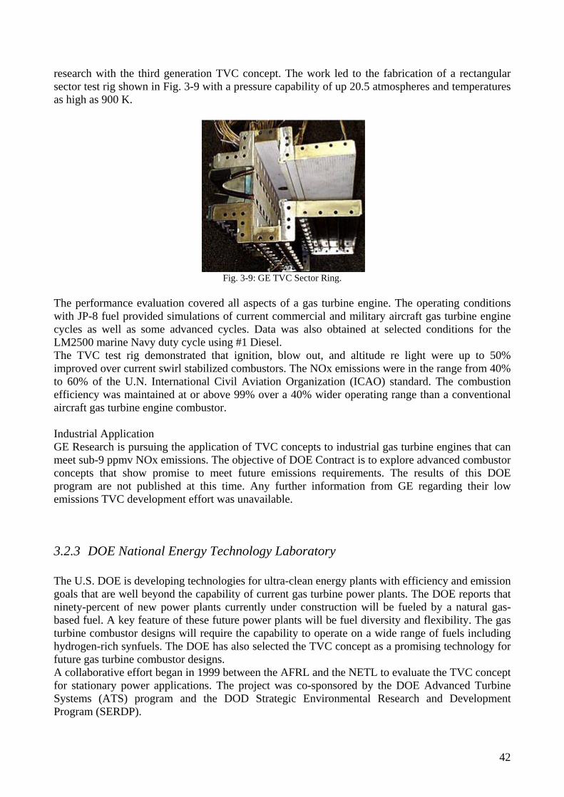
research with the third generation TVC concept. The work led to the fabrication of a rectangular sector test rig shown in Fig. 3-9 with a pressure capability of up 20.5 atmospheres and temperatures as high as 900 K.

Fig. 3-9: GE TVC Sector Ring.

The performance evaluation covered all aspects of a gas turbine engine. The operating conditions with JP-8 fuel provided simulations of current commercial and military aircraft gas turbine engine cycles as well as some advanced cycles. Data was also obtained at selected conditions for the LM2500 marine Navy duty cycle using #1 Diesel. The TVC test rig demonstrated that ignition, blow out, and altitude re light were up to 50% improved over current swirl stabilized combustors. The NOx emissions were in the range from 40% to 60% of the U.N. International Civil Aviation Organization (ICAO) standard. The combustion efficiency was maintained at or above 99% over a 40% wider operating range than a conventional aircraft gas turbine engine combustor. Industrial Application GE Research is pursuing the application of TVC concepts to industrial gas turbine engines that can meet sub-9 ppmv NOx emissions. The objective of DOE Contract is to explore advanced combustor concepts that show promise to meet future emissions requirements. The results of this DOE program are not published at this time. Any further information from GE regarding their low emissions TVC development effort was unavailable.

3.2.3 DOE National Energy Technology Laboratory The U.S. DOE is developing technologies for ultra-clean energy plants with efficiency and emission goals that are well beyond the capability of current gas turbine power plants. The DOE reports that ninety-percent of new power plants currently under construction will be fueled by a natural gas-based fuel. A key feature of these future power plants will be fuel diversity and flexibility. The gas turbine combustor designs will require the capability to operate on a wide range of fuels including hydrogen-rich synfuels. The DOE has also selected the TVC concept as a promising technology for future gas turbine combustor designs. A collaborative effort began in 1999 between the AFRL and the NETL to evaluate the TVC concept for stationary power applications. The project was co-sponsored by the DOE Advanced Turbine Systems (ATS) program and the DOD Strategic Environmental Research and Development Program (SERDP).

42

The primary intent was to assess the low-emissions capabilities of a novel RQL staged combustor shown in Fig. 3-10 [Straub 2000]. The goal was to achieve NOx and CO emissions that are comparable to other commercial natural gas burning DLN systems. High BTU-fuels and fuels containing significant amounts of fuel-bound nitrogen were evaluated. NETL has continued to pursue the development of TVC concepts and combustor configurations with their own internal research program and through separate collaborative projects with GE and Ramgen Power Systems (RPS). The recently released multi-year turbine development program is evidence that the DOE is committed to the advancement of novel combustor designs such as the TVC concept.

Fig. 3-10: NETL RQL TVC.

NETL and RPS with support from the California Energy Commission completed in early 2005 a series of rig tests that demonstrated less than 3 ppmv NOx at industrial gas turbine operating conditions without the need for a stabilizing catalyst or exhaust aftertreatment.

3.2.4 Ramgen Power Systems (RPS) RPS is pursuing the development of its unique Advanced Vortex Combustion (AVC) technology that has positive promise for improved efficiency, lower emissions, greater flame stability, fuel flexibility, increased durability, and reduced manufacturing costs. RPS is evaluating the potential for product insertion into a wide variety of industrial applications including gas turbine power generation and mechanical drive, manufacturing processing, chemical process heating, steam boiler systems, and incineration. The immediate AVC application is for low emissions stationary gas turbine engines. In 2002, RPS tested the first AVC concept (Fig. 3-11) with support from the DOE NETL and achieved 9 ppmv NOX emissions on natural gas in lean premixed mode [Bucher 2003].

Fig. 3-11: RPS AVC configuration.

The testing was conducted at the GASL facility in New York. The development of AVC concepts for gas turbine applications has continued since the test program at GASL. RPS and NETL with support from the CEC have recently completed a joint project that has shown tremendous promise for the AVC technology for extremely low emissions and acoustically stable combustion. These test results indicate the potential to achieve unprecedented emissions levels of 1 ppmv NOx and 9 ppmv CO at industrial gas turbine operating conditions.

43

The tests were conducted in the NETL Low Emissions Combustion Test and Research (LECTR) facility at 10 atmospheres with combustor inlet temperature of 329°C. The combustor is air-cooled

; Air-cooled combustor functioned as designed and without incident;

by video through the quartz window;

3 ppmv NOx and 20 ppmv CO;

t;

sertion opportunities in industrial applications including gas turbine power generation and

.2.5 ALM Turbines

ustor experts, including those at ALM Turbine Inc., are increasingly ptimistic about the promise of TVC [Kalin 2005]. It is ALM’s position that the TVC concept has

ating conditions.

temperature, is less than 2 milliseconds.

to closely simulate actual gas turbine conditions. The series of parametric tests allowed for variation in inlet pressure, fuel flow, air flow loading, lean blowout and pressure dynamics. A 4inch-by- 4inch quartz window allowed for flame visualization up to 5 atmospheres. The test results can be summarized as follows: • Data taken at 10 atmospheres and 329°C•• Combustor ignited at ambient conditions; • System was stable throughout start-up and shut-down; • Flame structure was observed and recorded• Overall combustor pressure drop was less than 2.6%; • NOx emissions are not pressure dependent under ultra-lean conditions; • Lowest measured NOx with acceptable CO emissions:• Combustion efficiencies greater than 99.9%; • Recorded combustion pressure oscillations with high frequency probe were insignifican RPS will continue to advance the development of its AVC technology and identify product inmechanical drive applications. The AVC technology is scalable to various sizes and heat load capabilities.

3 Many turbine and combomany real potential advantages over both diffusion flame and DLN combustors, including lower emissions, multi-fuel capability, better flame stability, uniformity of flame, better dynamics, greater lean blowout limit offering greater turndown, higher efficiency due to lower combustor pressure drop losses, compactness, and lower manufacturing costs. Over the last few years, ALM has designed, manufactured and tested a number of proprietary prototype TVCs that have demonstrated many of the above mentioned advantages. ALM has been developing and testing its own proprietary version of TVC for both microturbines and large MW scale industrial turbines. In 2003, ALM and Alturdyne successfully designed, manufactured, and incorporated a TVC combustor into a Sunstrand T-62 APU. ALM has also designed, manufactured and rig tested two MW scale prototypes at ambient conditions that meet GE 7E 85MW operThe ALM TVC consists of two autonomous sections – a thermal nozze and vortex (Fig. 3-12). The time of complete fuel burning, at the primary combustionALM has achieved combustion at very low temperatures without use of any catalysts. The ALM design is notably different from all other TVC concepts. The concept utilizes its vortex and manages the recirculation flows in a different manner. The combustion mainly takes place in the thermal nozzle and not in the vortex.

44

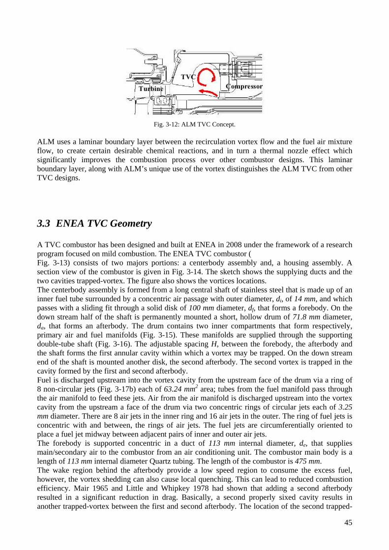
Fig. 3-12: ALM TVC Concept.

ALM uses a laminar boundary layer between the recirculation vortex flow and the fuel air mixture flow, to create certain desirable chemical reactions, and in turn a thermal nozzle effect which significantly improves the combustion process over other combustor designs. This laminar boundary layer, along with ALM’s unique use of the vortex distinguishes the ALM TVC from other TVC designs.

3.3 ENEA TVC Geometry A TVC combustor has been designed and built at ENEA in 2008 under the framework of a research program focused on mild combustion. The ENEA TVC combustor ( Fig. 3-13) consists of two majors portions: a centerbody assembly and, a housing assembly. A section view of the combustor is given in Fig. 3-14. The sketch shows the supplying ducts and the two cavities trapped-vortex. The figure also shows the vortices locations. The centerbody assembly is formed from a long central shaft of stainless steel that is made up of an inner fuel tube surrounded by a concentric air passage with outer diameter, di, of 14 mm, and which passes with a sliding fit through a solid disk of 100 mm diameter, df, that forms a forebody. On the down stream half of the shaft is permanently mounted a short, hollow drum of 71.8 mm diameter, da, that forms an afterbody. The drum contains two inner compartments that form respectively, primary air and fuel manifolds (Fig. 3-15). These manifolds are supplied through the supporting double-tube shaft (Fig. 3-16). The adjustable spacing H, between the forebody, the afterbody and the shaft forms the first annular cavity within which a vortex may be trapped. On the down stream end of the shaft is mounted another disk, the second afterbody. The second vortex is trapped in the cavity formed by the first and second afterbody. Fuel is discharged upstream into the vortex cavity from the upstream face of the drum via a ring of 8 non-circular jets (Fig. 3-17b) each of 63.24 mm2 area; tubes from the fuel manifold pass through the air manifold to feed these jets. Air from the air manifold is discharged upstream into the vortex cavity from the upstream a face of the drum via two concentric rings of circular jets each of 3.25 mm diameter. There are 8 air jets in the inner ring and 16 air jets in the outer. The ring of fuel jets is concentric with and between, the rings of air jets. The fuel jets are circumferentially oriented to place a fuel jet midway between adjacent pairs of inner and outer air jets. The forebody is supported concentric in a duct of 113 mm internal diameter, de, that supplies main/secondary air to the combustor from an air conditioning unit. The combustor main body is a length of 113 mm internal diameter Quartz tubing. The length of the combustor is 475 mm. The wake region behind the afterbody provide a low speed region to consume the excess fuel, however, the vortex shedding can also cause local quenching. This can lead to reduced combustion efficiency. Mair 1965 and Little and Whipkey 1978 had shown that adding a second afterbody resulted in a significant reduction in drag. Basically, a second properly sixed cavity results in another trapped-vortex between the first and second afterbody. The location of the second trapped-

45

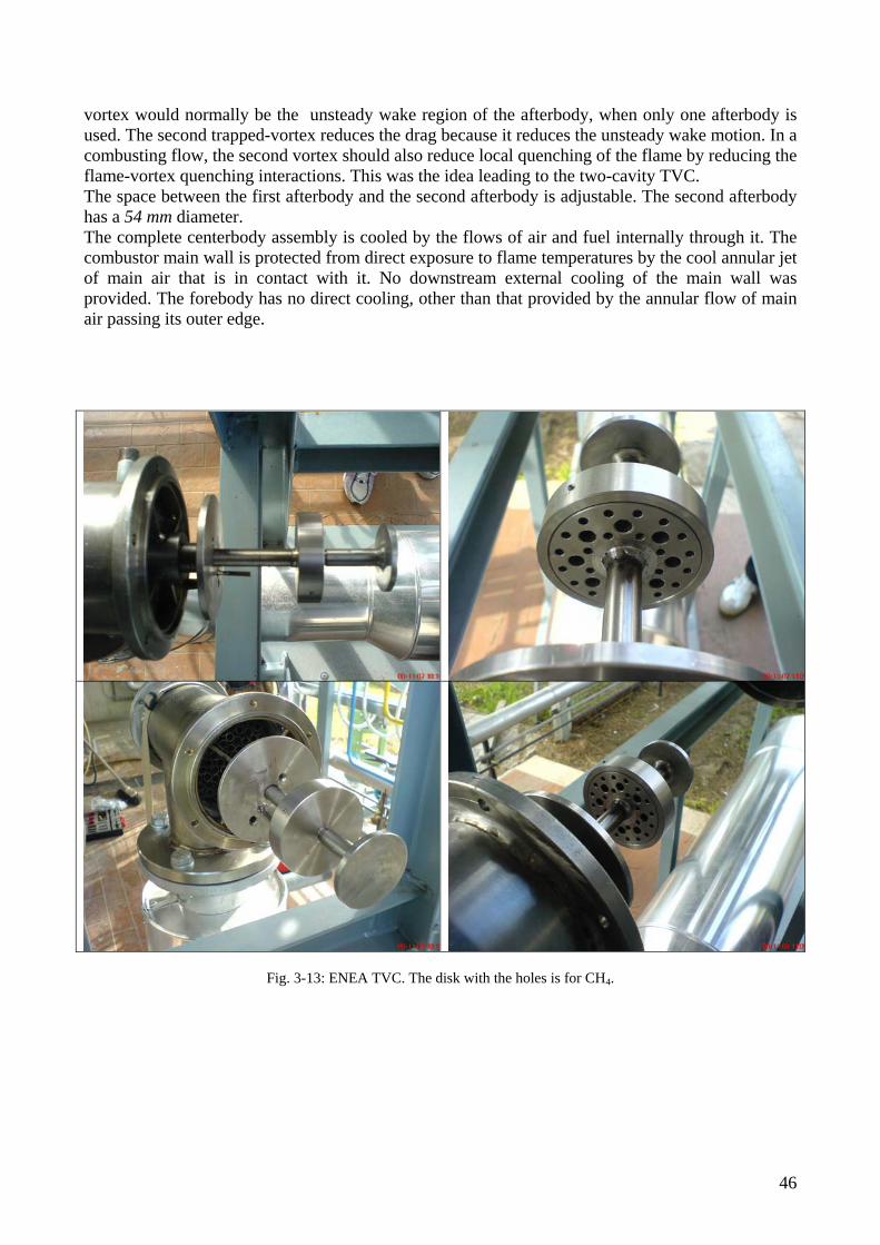
vortex would normally be the unsteady wake region of the afterbody, when only one afterbody is used. The second trapped-vortex reduces the drag because it reduces the unsteady wake motion. In a combusting flow, the second vortex should also reduce local quenching of the flame by reducing the flame-vortex quenching interactions. This was the idea leading to the two-cavity TVC. The space between the first afterbody and the second afterbody is adjustable. The second afterbody has a 54 mm diameter. The complete centerbody assembly is cooled by the flows of air and fuel internally through it. The combustor main wall is protected from direct exposure to flame temperatures by the cool annular jet of main air that is in contact with it. No downstream external cooling of the main wall was provided. The forebody has no direct cooling, other than that provided by the annular flow of main air passing its outer edge.

Fig. 3-13: ENEA TVC. The disk with the holes is for CH4.

46

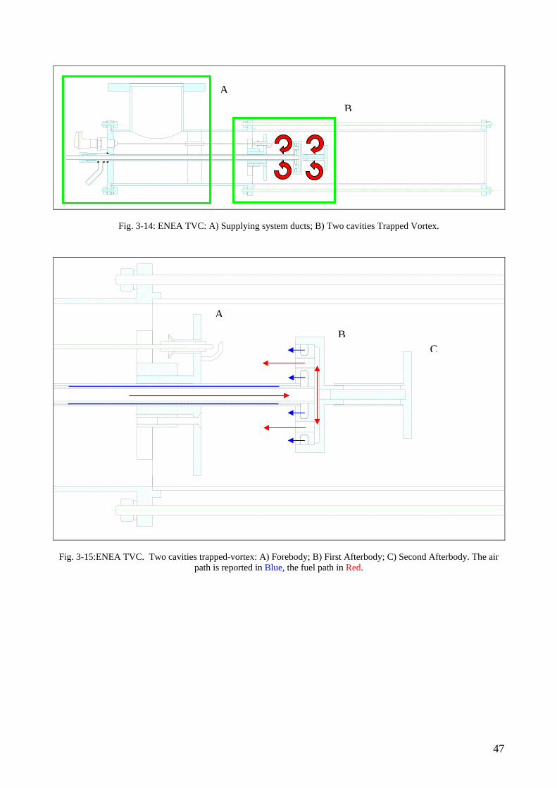
A

B

Fig. 3-14: ENEA TVC: A) Supplying system ducts; B) Two cavities Trapped Vortex.

A

BC

Fig. 3-15:ENEA TVC. Two cavities trapped-vortex: A) Forebody; B) First Afterbody; C) Second Afterbody. The air

path is reported in Blue, the fuel path in Red.

47

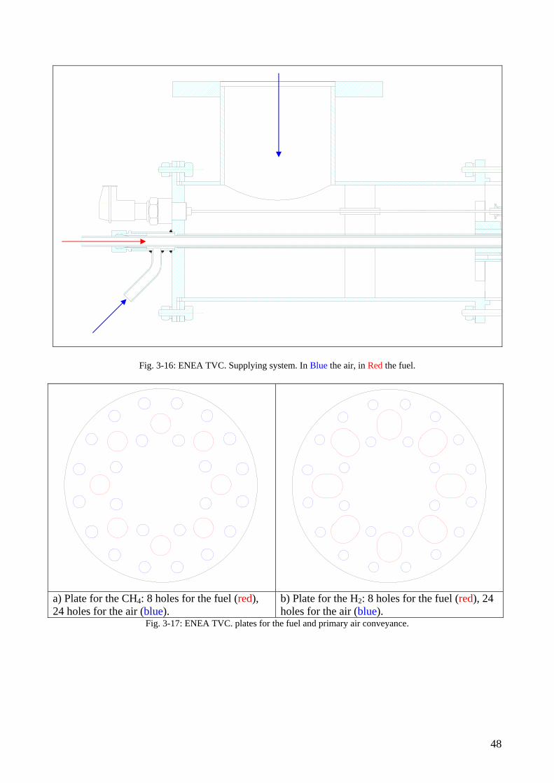
Fig. 3-16: ENEA TVC. Supplying system. In Blue the air, in Red the fuel.

a) Plate for the CH4: 8 holes for the fuel (red), 24 holes for the air (blue).

b) Plate for the H2: 8 holes for the fuel (red), 24 holes for the air (blue).

Fig. 3-17: ENEA TVC. plates for the fuel and primary air conveyance.

48

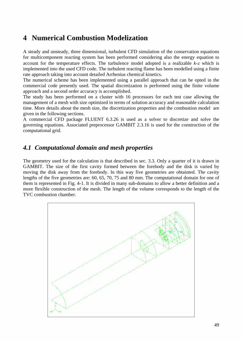
4 Numerical Combustion Modelization A steady and unsteady, three dimensional, turbulent CFD simulation of the conservation equations for multicomponent reacting system has been performed considering also the energy equation to account for the temperature effects. The turbulence model adopted is a realizable k-ε which is implemented into the used CFD code. The turbulent reacting flame has been modelled using a finite rate approach taking into account detailed Arrhenius chemical kinetics. The numerical scheme has been implemented using a parallel approach that can be opted in the commercial code presently used. The spatial discretization is performed using the finite volume approach and a second order accuracy is accomplished. The study has been performed on a cluster with 16 processors for each test case allowing the management of a mesh with size optimized in terms of solution accuracy and reasonable calculation time. More details about the mesh size, the discretization properties and the combustion model are given in the following sections. A commercial CFD package FLUENT 6.3.26 is used as a solver to discretize and solve the governing equations. Associated preprocessor GAMBIT 2.3.16 is used for the construction of the computational grid.

4.1 Computational domain and mesh properties The geometry used for the calculation is that described in sec. 3.3. Only a quarter of it is drawn in GAMBIT. The size of the first cavity formed between the forebody and the disk is varied by moving the disk away from the forebody. In this way five geometries are obtainted. The cavity lengths of the five geometries are: 60, 65, 70, 75 and 80 mm. The computational domain for one of them is represented in Fig. 4-1. It is divided in many sub-domains to allow a better definition and a more flexible construction of the mesh. The length of the volume corresponds to the length of the TVC combustion chamber.

49

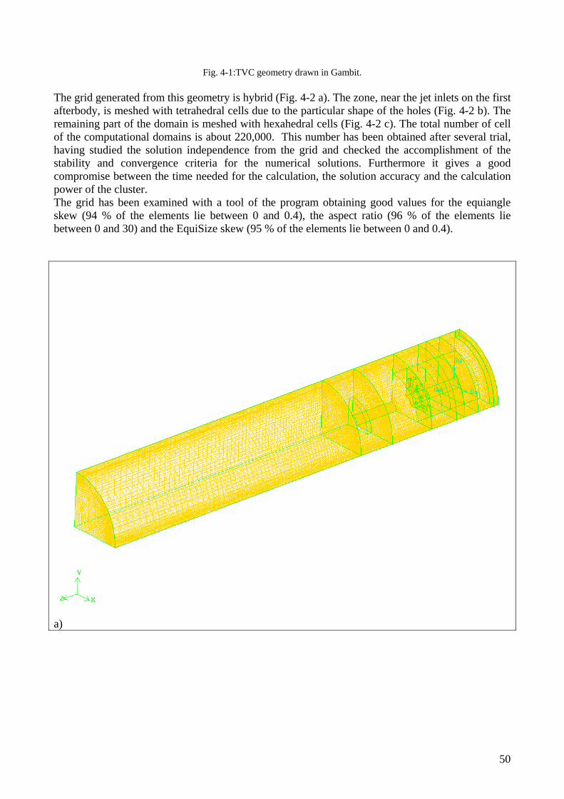
Fig. 4-1:TVC geometry drawn in Gambit. The grid generated from this geometry is hybrid (Fig. 4-2 a). The zone, near the jet inlets on the first afterbody, is meshed with tetrahedral cells due to the particular shape of the holes (Fig. 4-2 b). The remaining part of the domain is meshed with hexahedral cells (Fig. 4-2 c). The total number of cell of the computational domains is about 220,000. This number has been obtained after several trial, having studied the solution independence from the grid and checked the accomplishment of the stability and convergence criteria for the numerical solutions. Furthermore it gives a good compromise between the time needed for the calculation, the solution accuracy and the calculation power of the cluster. The grid has been examined with a tool of the program obtaining good values for the equiangle skew (94 % of the elements lie between 0 and 0.4), the aspect ratio (96 % of the elements lie between 0 and 30) and the EquiSize skew (95 % of the elements lie between 0 and 0.4).

a)

50

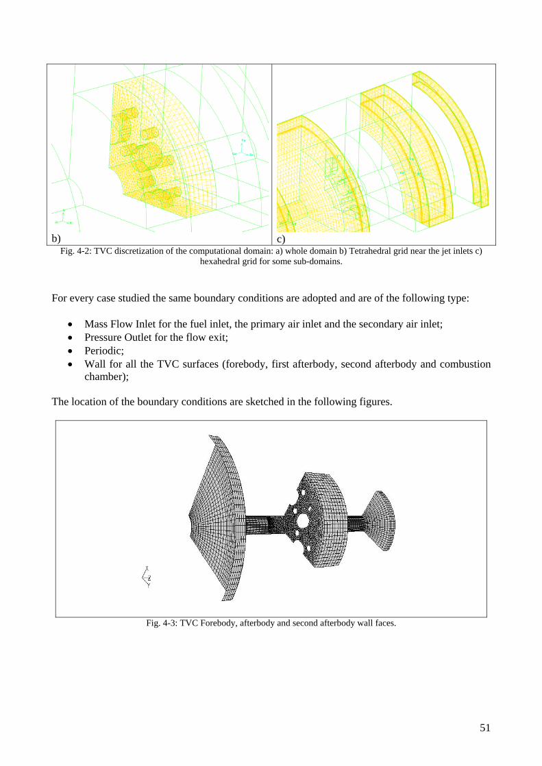
b) c) Fig. 4-2: TVC discretization of the computational domain: a) whole domain b) Tetrahedral grid near the jet inlets c)

hexahedral grid for some sub-domains. For every case studied the same boundary conditions are adopted and are of the following type:

• Mass Flow Inlet for the fuel inlet, the primary air inlet and the secondary air inlet; • Pressure Outlet for the flow exit; • Periodic; • Wall for all the TVC surfaces (forebody, first afterbody, second afterbody and combustion

chamber); The location of the boundary conditions are sketched in the following figures.

Fig. 4-3: TVC Forebody, afterbody and second afterbody wall faces.

51

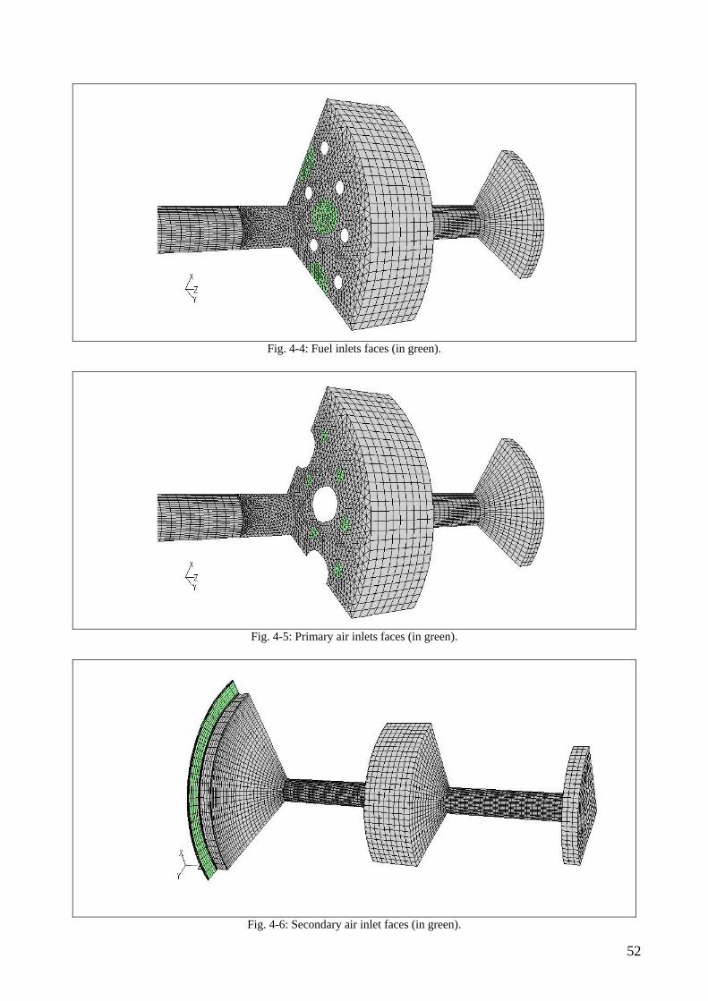
Fig. 4-4: Fuel inlets faces (in green).

Fig. 4-5: Primary air inlets faces (in green).

Fig. 4-6: Secondary air inlet faces (in green).

52

Fig. 4-7: Periodic boundary faces (in cyan).

Fig. 4-8: Combustion chamber wall faces and pressure outlet faces (in red).

4.2 Numerical model This section examines the numerical model, showing some steps in the setup and solution procedure used for the TVC combustion computations. The code uses a control-volume based technique to convert a general scalar transport equation to an algebraic equation. The control technique consists of integrating the transport equation about each control volume, yielding a discrete equation that expresses the conservation law on a control-volume basis. The solver adopted is a pressure based solver with an implicit formulation. The pressure-based solver employs an algorithm which belongs to a general class of methods called the projection method. In the projection method, wherein the constraint of mass conservation (continuity) of the velocity field is achieved by solving a pressure (or pressure correction) equation. The pressure equation is derived from the continuity and the momentum equations in such a way that the velocity

53

field, corrected by the pressure, satisfies the continuity. Since the governing equations are nonlinear and coupled to one another, the solution process involves iterations wherein the entire set of governing equations is solved repeatedly until the solution converges. The governing equations solved in the simulations are the continuity, momentum, energy, radiation, turbulence and species conservation equations. The models for the, turbulence radiation, and combustion are reported in the following sections with a brief discussion on the theoretical back ground. Then the mixture species and material properties together with the boundary conditions are explicitly described.

4.2.1 Realizable k-ε This section presents the essential features of the turbulence model: the realizable k-ε model. The model is very similar to the standard k-ε. It also have the two transport equations for k and ε. The realizable k-ε model is a relatively recent development and differs from the standard model in two important ways:

• The realizable k-ε model contains a new formulation for the turbulent viscosity. • A new transport equation for the dissipation rate, ε, has been derived from an exact equation

for the transport of the mean-square vorticity fluctuation. The term “realizable” means that the model satisfies certain mathematical constraints on the Reynolds stresses, consistent with physics of turbulent flows. The other known models (standard or RNG) are not realizable. And immediate benefit of the realizable k-ε model is that it more accurately predicts the spreading rate of both planar and round jets. It is also likely to provide superior performance for flows involving rotation, boundary layers under strong adverse pressure gradients, separation, and recirculation. The realizable k-ε model has shown substantial improvements over the standard k-ε model where the flow features include strong streamline curvature, vortices and rotation. The modelled transport equation for k and ε in the realizable k-ε are:

( ) ( ) kMbkik

t

ii

i

SYGGxk

xkx

xk

t+−−++⎥

⎦

⎤⎢⎣

⎡

∂∂

⎟⎟⎠

⎞⎜⎜⎝

⎛+

∂∂

=∂∂

+∂∂ ρε

σμ

μρρ 4-1

and

( ) ( ) εεεε

ενε

ερερεσμ

μρερε SGCk

Ck

CSCxx

uxt b

i

t

ii

i

+++

−+⎥⎦

⎤⎢⎣

⎡

∂∂

⎟⎟⎠

⎞⎜⎜⎝

⎛+

∂∂

=∂∂

+∂∂

31

2

21 4-2

Where

⎥⎦

⎤⎢⎣

⎡+

=5

,43.0max1 ηηC ,

εη kS= , ijij SSS = 4-3

54

In these equations, Gk represents the generation of turbulence kinetic energy due to the mean velocity gradients. Gb is the generation of turbulence kinetic energy due to buoyancy. YM represents the contribution of the fluctuating dilatation in compressible turbulence to the overall dissipation rate. C2 and C1ε are constants. σk and σε are the turbulent Prandtl numbers for k and ε, respectively. Sk and Sε are the source terms. The model constants can be varied in order to ensure good performance with the flow under consideration. As in the other models the turbulent viscosity is calculated with:

ερμ μ

2kCt = 4-4

but the Cμ is no longer constant and it is computed as a function of the mean strain and rotation rates, the angular velocity of the system rotation and the turbulence fields.

4.2.2 Radiation model In Fluent there are five radiation models which allow to include radiation in the heat transfer simulations. Depending on the problem one radiation model may be more appropriate than the others. In the case take into consideration here the choice is the Discrete Ordinates (DO) model. The DO model spans the entire range of optical thicknesses, and allow to solve problems ranging from surface to surface radiation to participating radiation in combustion problems. The DO radiation model solves the radiative transfer equation (RTE) for a finite number of discrete solid angles, each associated with a vector direction fixed in the global Cartesian system. The finesses of the angular discretization is controlled by the user. The DO model transform the RTE equation:

( ) ( ) ( ) ( ) ( )∫ Ω⋅Θ+=++π

πσ

πσσ

4

0

42 '',

4,, dsssrITansrIa

dssrdI s

srrrrrr

rr

4-5

Where: rr is the position vector; srr is the direction vector; 's is the scattering direction vector;

s is the path length; a is the absorption coefficient; n is the refractive index; σs is the scattering coefficient; σ is the Stefan-Boltzmann constant; I is the radiation intensity; T is the local temperature

is the phase function; Θ is the solid angle; 'Ω

into a transport equation for radiation intensity in the spatial coordinates. Thus, the equation 4-5 can be written as:

55

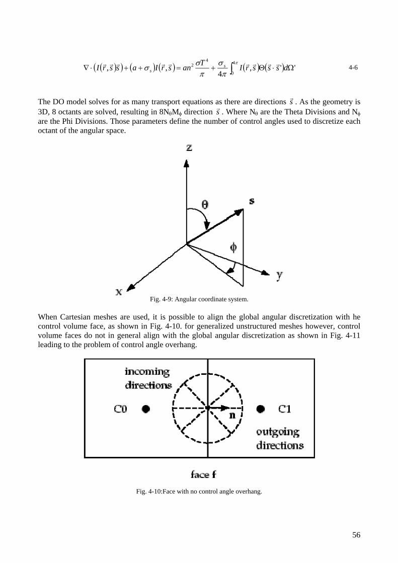
( )( ) ( ) ( ) ( ) ( )∫ Ω⋅Θ+=++⋅∇π

πσ

πσσ

4

0

42 '',

4,, dsssrITansrIassrI s

srrrrrrrrr 4-6

The DO model solves for as many transport equations as there are directions s . As the geometry is 3D, 8 octants are solved, resulting in 8NθMφ direction

r

sr . Where Nθ are the Theta Divisions and Nφ are the Phi Divisions. Those parameters define the number of control angles used to discretize each octant of the angular space.

Fig. 4-9: Angular coordinate system.

When Cartesian meshes are used, it is possible to align the global angular discretization with he control volume face, as shown in Fig. 4-10. for generalized unstructured meshes however, control volume faces do not in general align with the global angular discretization as shown in Fig. 4-11 leading to the problem of control angle overhang.

Fig. 4-10:Face with no control angle overhang.

56

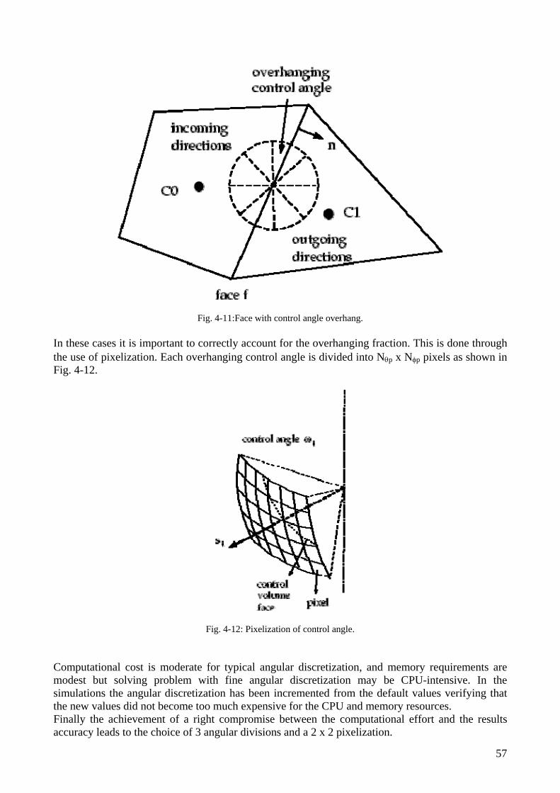
Fig. 4-11:Face with control angle overhang. In these cases it is important to correctly account for the overhanging fraction. This is done through the use of pixelization. Each overhanging control angle is divided into Nθp x Nφp pixels as shown in Fig. 4-12.

Fig. 4-12: Pixelization of control angle. Computational cost is moderate for typical angular discretization, and memory requirements are modest but solving problem with fine angular discretization may be CPU-intensive. In the simulations the angular discretization has been incremented from the default values verifying that the new values did not become too much expensive for the CPU and memory resources. Finally the achievement of a right compromise between the computational effort and the results accuracy leads to the choice of 3 angular divisions and a 2 x 2 pixelization.

57

The DO model also allows the solution of radiation at semi-transparent walls and opaque walls. In this way the right amount of absorbed, emitted and reflected energy from the wall surface can be taken into account. The TVC forebody, first afterbody and second afterbody walls are considered as opaque walls made in steel while the TVC combustion chamber, made in quartz, is considered as semi-transparent. All the physical and thermal properties of the steel and quartz are properly set in the code (see next table).

Steel Quartz Density [kg/m3] 8030 2203Specific heat [J/kg-K] 502 703Thermal conductivity [W/m-K] 16.27 1.33Refractive index - 1.46Emissivity 0.8 0.93Tab. 4-1:Steel and quartz thermal and physical properties.

4.2.3 Combustion Model The combustion process in the TVC is solved using a finite rate reaction model based on the Arrhenius equation: the Eddy Dissipation Concept (EDC). It is an extension of the eddy dissipation model to include detailed chemical mechanism in turbulent flows. The detailed mechanism has been reported in sec. 2.3.2. The assumptions, on which the model resides, can be resumed in:

• In turbulent flow, the chemical reactions takes place where reactants or reactants and hot products are molecularly mixed.

• In turbulent flow the molecular mixing takes place where dissipation of turbulent kinetic energy takes place.

• Turbulent kinetic energy is transported from energy containing large turbulent structures to intermittently distributed fine structures with high mixing where the kinetic energy is dissipated into heat.

• The dissipative fine structures are intermittently distributed. • Only a fraction of the dissipative structures is burning, the burning fine structures

Thus the model assumes that chemical reactions occur within the smallest turbulent structures, called fine structures. Due to intense mixing in the dissipative structure, these are treated as perfectly stirred reactors (PSR) which exchange mass with the surrounding fluid. The overall reaction rate in each PSR is controlled by chemical kinetics. The properties of the fine structures are derived from a step-wise energy cascade model and expressed with quantities related to the main flow, such as the turbulent kinetic energy, k, and the turbulent dissipation rate, ε. Due to the preceding assumptions, the reaction rate in the fine structures perfectly stirred reactors can easily be modelled as the change in mass fraction through the fine structure reactors divided by the residence time of these reactors. The mean reaction rates are then modelled as the reaction rates of the burning fine structures times the mass fraction of the burning fine structures [Magnussen]. The EDC model is needed to compute the reaction rate (Ri) appearing as source term in:

58

( ) ( ) iiiii SRJYvYt

++⋅−∇=⋅∇+∂∂ rrρρ

The conservation equation for the ith chemical species. Si is the rate of creation by addition from the dispersed phase.

iJr

is the diffusion flux of species i, which arise due to concentration gradients. In laminar flows using the dilute approximation it can be written as:

imii YDJ ∇−= ,ρr

Di,m is the diffusion coefficient for species i in the mixture. While in turbulent flows it is:

it

tmii Y

ScDJ ∇⎟⎟

⎠

⎞⎜⎜⎝

⎛+−=

μρ ,

r

Where Sct is the turbulent Schmidt number which by default is 0.7. The EDC assumes that reaction occurs in small turbulent structures, called fine scales. The length fraction of the fine scales is modelled as:

4/1

2* ⎟⎠⎞

⎜⎝⎛=

kC νεξ ξ

Where * denotes the fine scales quantities, Cξ is the volume fraction constant and k and ε are obtained from the turbulence model. Species are assumed to react in the fine structures over a time scale

2/1

* ⎟⎠⎞

⎜⎝⎛=

εντ τC

Where Cτ is the time scale constant. τ* is controlled by the chemical kinetics. Using the previous definitions the source term in the conservation equation for the mean species i, is modelled as

( )( )[ ]( )iii YYR −

−= *

*1**

3

2

ξτξρ

Where Y*i is the fine scale species mass fraction after reacting over the time τ*.

4.2.4 Gas Mixture Properties The gas mixture is composed by 13 species: H H2 H2O H2O2 HO2 HNO N N2 N2O NO O O2 OH. For each species in the gas mixture the properties in the following tables are set:

59

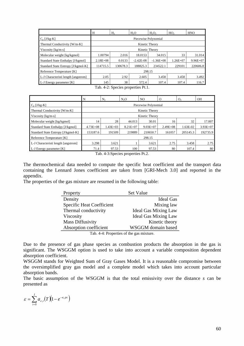
H H2 H2O H2O2 HO2 HNO

Cp [J/kg-K] Piecewise Polynomial

Thermal Conductivity [W/m-K] Kinetic Theory

Viscosity [kg/m-s] Kinetic Theory

Molecular weight [kg/kgmol] 1.00794 2.016 18.0153 34.015 33 31.014

Standard State Enthalpy [J/kgmol] 2.18E+08 0.0133 -2.42E-08 -1.36E+08 1.26E+07 9.96E+07

Standard State Entropy [J/kgmol-K] 114715.5 130678.3 188825.3 234522.1 229101 220606.8

Reference Temperature [K] 298.15

L-J Characteristi length [angstrom] 2.05 2.92 2.605 3.458 3.458 3.492

L-J Energy parameter [K] 145 38 572.4 107.4 107.4 116.7Tab. 4-2: Species properties Pt.1.

N N2 N2O NO O O2 OH

Cp [J/kg-K] Piecewise Polynomial

Thermal Conductivity [W/m-K] Kinetic Theory

Viscosity [kg/m-s] Kinetic Theory

Molecular weight [kg/kgmol] 14 28 44.013 30.01 16 32 17.007

Standard State Enthalpy [J/kgmol] 4.73E+08 1.43E+03 8.21E+07 9.03E+07 2.49E+08 1.63E-02 3.93E+07

Standard State Entropy [J/kgmol-K] 153187.6 191509 219889 210650.7 161057 205145.3 192735.9

Reference Temperature [K] 298.15

L-J Characteristi length [angstrom] 3.298 3.621 1 3.621 2.75 3.458 2.75

L-J Energy parameter [K] 71.4 97.53 100 97.53 80 107.4 80Tab. 4-3:Species properties Pt.2.

The thermochemical data needed to compute the specific heat coefficient and the transport data containing the Lennard Jones coefficient are taken from [GRI-Mech 3.0] and reported in the appendix. The properties of the gas mixture are resumed in the following table:

Property Set Value Density Ideal Gas Specific Heat Coefficient Mixing law Thermal conductivity Ideal Gas Mixing Law Viscosity Ideal Gas Mixing Law Mass Diffusivity Kinetic theory Absorption coefficient WSGGM domain based

Tab. 4-4: Properties of the gas mixture. Due to the presence of gas phase species as combustion products the absorption in the gas is significant. The WSGGM option is used to take into account a variable composition dependent absorption coefficient. WSGGM stands for Weighted Sum of Gray Gases Model. It is a reasonable compromise between the oversimplified gray gas model and a complete model which takes into account particular absorption bands. The basic assumption of the WSGGM is that the total emissivity over the distance s can be presented as

( )( )∑=

−−=I

i

psi

ieTa0

, 1 κεε

60

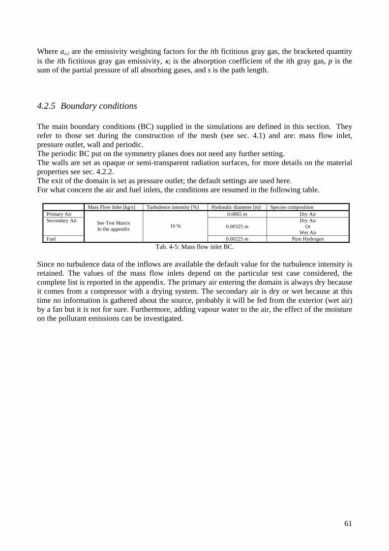
Where aε,i are the emissivity weighting factors for the ith fictitious gray gas, the bracketed quantity is the ith fictitious gray gas emissivity, κi is the absorption coefficient of the ith gray gas, p is the sum of the partial pressure of all absorbing gases, and s is the path length.

4.2.5 Boundary conditions The main boundary conditions (BC) supplied in the simulations are defined in this section. They refer to those set during the construction of the mesh (see sec. 4.1) and are: mass flow inlet, pressure outlet, wall and periodic. The periodic BC put on the symmetry planes does not need any further setting. The walls are set as opaque or semi-transparent radiation surfaces, for more details on the material properties see sec. 4.2.2. The exit of the domain is set as pressure outlet; the default settings are used here. For what concern the air and fuel inlets, the conditions are resumed in the following table.

Mass Flow Inlet [kg/s] Turbulence intensity [%] Hydraulic diameter [m] Species composition Primary Air 0.0065 m Dry Air Secondary Air

0.00325 m Dry Air

Or Wet Air

Fuel

See Test Matrix In the appendix 10 %

0.00225 m Pure Hydrogen Tab. 4-5: Mass flow inlet BC.

Since no turbulence data of the inflows are available the default value for the turbulence intensity is retained. The values of the mass flow inlets depend on the particular test case considered, the complete list is reported in the appendix. The primary air entering the domain is always dry because it comes from a compressor with a drying system. The secondary air is dry or wet because at this time no information is gathered about the source, probably it will be fed from the exterior (wet air) by a fan but it is not for sure. Furthermore, adding vapour water to the air, the effect of the moisture on the pollutant emissions can be investigated.

61

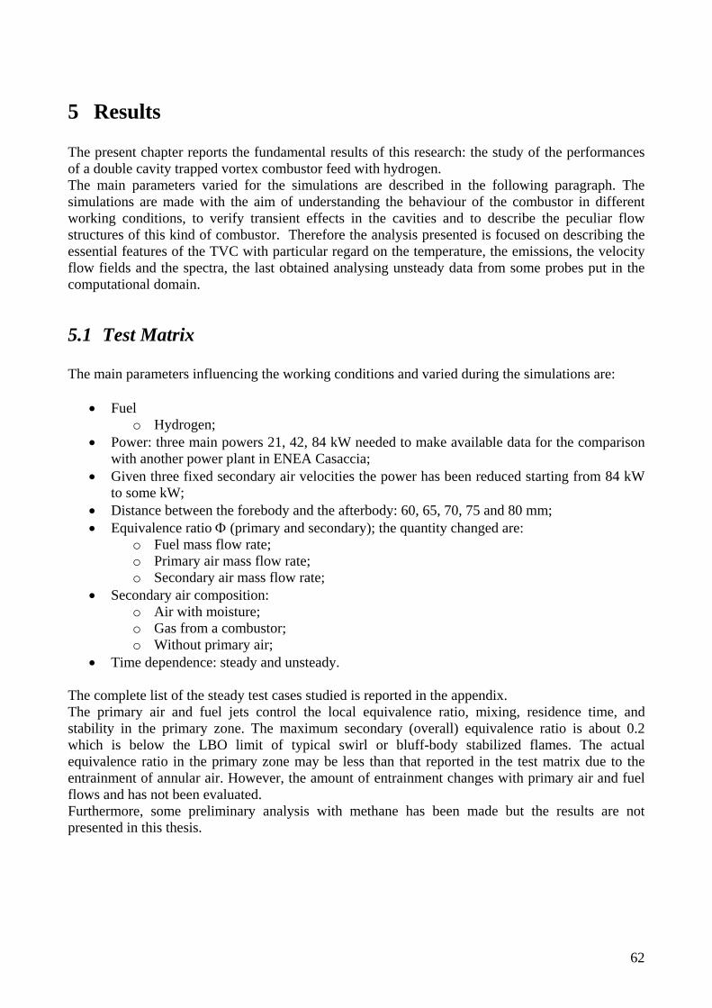
5 Results The present chapter reports the fundamental results of this research: the study of the performances of a double cavity trapped vortex combustor feed with hydrogen. The main parameters varied for the simulations are described in the following paragraph. The simulations are made with the aim of understanding the behaviour of the combustor in different working conditions, to verify transient effects in the cavities and to describe the peculiar flow structures of this kind of combustor. Therefore the analysis presented is focused on describing the essential features of the TVC with particular regard on the temperature, the emissions, the velocity flow fields and the spectra, the last obtained analysing unsteady data from some probes put in the computational domain.

5.1 Test Matrix The main parameters influencing the working conditions and varied during the simulations are:

• Fuel o Hydrogen;

• Power: three main powers 21, 42, 84 kW needed to make available data for the comparison with another power plant in ENEA Casaccia;

• Given three fixed secondary air velocities the power has been reduced starting from 84 kW to some kW;

• Distance between the forebody and the afterbody: 60, 65, 70, 75 and 80 mm; • Equivalence ratio Φ (primary and secondary); the quantity changed are:

o Fuel mass flow rate; o Primary air mass flow rate; o Secondary air mass flow rate;

• Secondary air composition: o Air with moisture; o Gas from a combustor; o Without primary air;

• Time dependence: steady and unsteady. The complete list of the steady test cases studied is reported in the appendix. The primary air and fuel jets control the local equivalence ratio, mixing, residence time, and stability in the primary zone. The maximum secondary (overall) equivalence ratio is about 0.2 which is below the LBO limit of typical swirl or bluff-body stabilized flames. The actual equivalence ratio in the primary zone may be less than that reported in the test matrix due to the entrainment of annular air. However, the amount of entrainment changes with primary air and fuel flows and has not been evaluated. Furthermore, some preliminary analysis with methane has been made but the results are not presented in this thesis.

62

5.2 Flow field and flame The flowfield in a small or large cavities is quite complex as a result of the formation of several vortices. Because of the presence of the cavities, the secondary air is expanded toward the centerbody, which, in turn, results in flow separations on the outer wall. The CFD solutions do provide valuable qualitative information to more fully understand the vortex structures in the cavities and the flow separations, but the present simulations predict only the large-scale vortical structures in the cavity, small scales important for mixing on a local level are not resolved. Fig. 5-1 shows the trapped vortices behind the TVC disks. As can be seen in the figure, several distinct vortices are predicted in the TVC cavities. The velocity field shows a strong recirculating flow that is expected for toroidal vortices. The main vortex in the first cavity rotates with the secondary air flow direction Fig. 5-2a due to the placement of the fuel and air injection points. But depending on the location and flow rates of the injection points, cavity vortices rotating in opposition or with the secondary air flow direction can be generated [Straub et al. 2000]. The vortices in the second cavity Fig. 5-2b and behind the second afterbody Fig. 5-2c also rotate with the annular air flow.

Fig. 5-1: TVC Velocity Pathlines. Test case: TVC-1.

a)

63

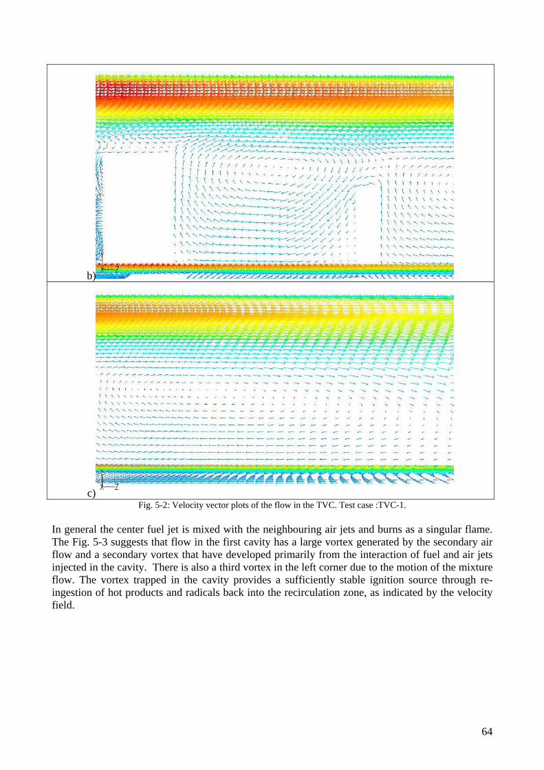
b)

c) Fig. 5-2: Velocity vector plots of the flow in the TVC. Test case :TVC-1.

In general the center fuel jet is mixed with the neighbouring air jets and burns as a singular flame. The Fig. 5-3 suggests that flow in the first cavity has a large vortex generated by the secondary air flow and a secondary vortex that have developed primarily from the interaction of fuel and air jets injected in the cavity. There is also a third vortex in the left corner due to the motion of the mixture flow. The vortex trapped in the cavity provides a sufficiently stable ignition source through re-ingestion of hot products and radicals back into the recirculation zone, as indicated by the velocity field.

64

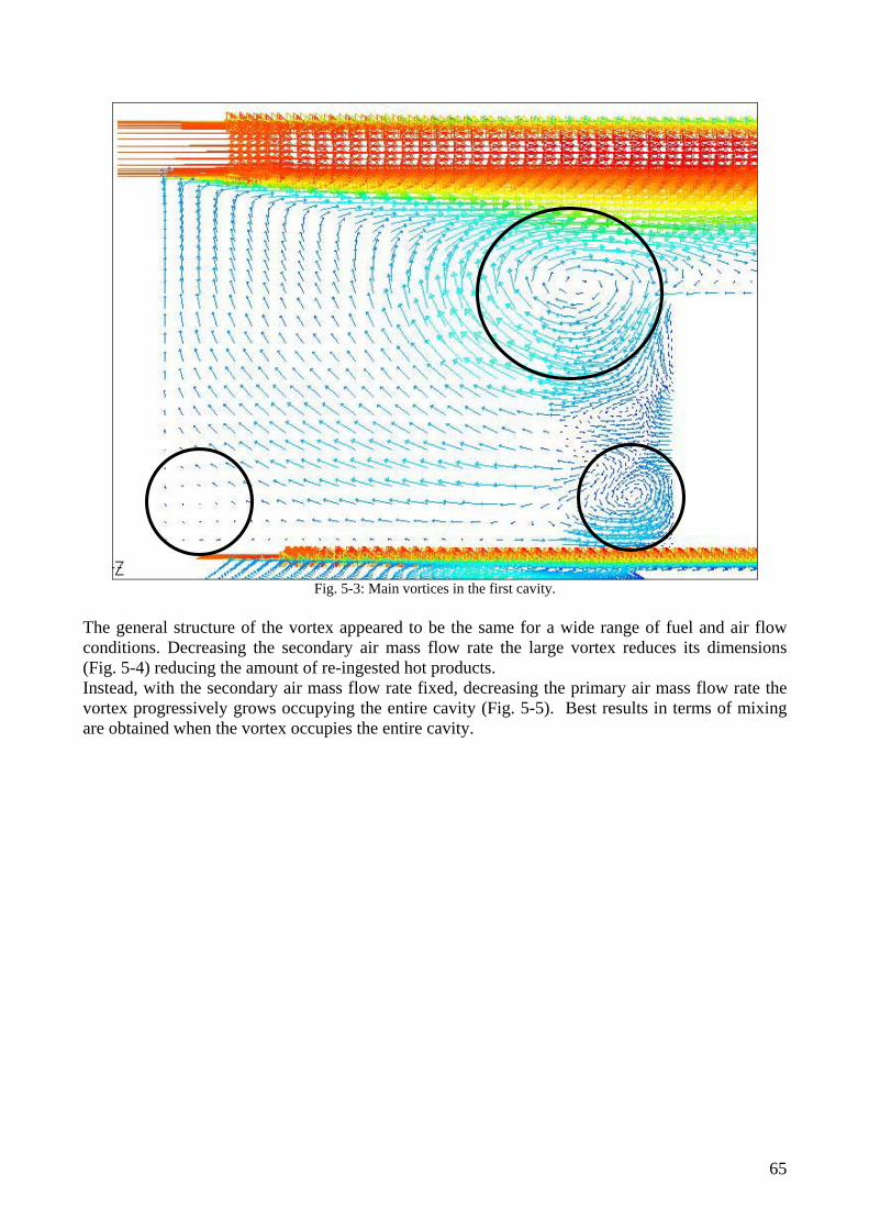
Fig. 5-3: Main vortices in the first cavity.

The general structure of the vortex appeared to be the same for a wide range of fuel and air flow conditions. Decreasing the secondary air mass flow rate the large vortex reduces its dimensions (Fig. 5-4) reducing the amount of re-ingested hot products. Instead, with the secondary air mass flow rate fixed, decreasing the primary air mass flow rate the vortex progressively grows occupying the entire cavity (Fig. 5-5). Best results in terms of mixing are obtained when the vortex occupies the entire cavity.

65

Fig. 5-4: Effect of the secondary air mass flow rate reduction on the trapped vortex dimensions.

66

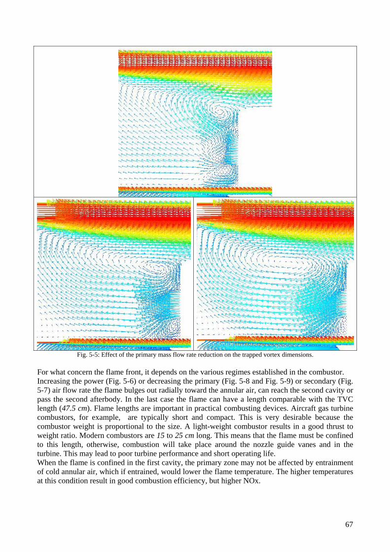
Fig. 5-5: Effect of the primary mass flow rate reduction on the trapped vortex dimensions. For what concern the flame front, it depends on the various regimes established in the combustor. Increasing the power (Fig. 5-6) or decreasing the primary (Fig. 5-8 and Fig. 5-9) or secondary (Fig. 5-7) air flow rate the flame bulges out radially toward the annular air, can reach the second cavity or pass the second afterbody. In the last case the flame can have a length comparable with the TVC length (47.5 cm). Flame lengths are important in practical combusting devices. Aircraft gas turbine combustors, for example, are typically short and compact. This is very desirable because the combustor weight is proportional to the size. A light-weight combustor results in a good thrust to weight ratio. Modern combustors are 15 to 25 cm long. This means that the flame must be confined to this length, otherwise, combustion will take place around the nozzle guide vanes and in the turbine. This may lead to poor turbine performance and short operating life. When the flame is confined in the first cavity, the primary zone may not be affected by entrainment of cold annular air, which if entrained, would lower the flame temperature. The higher temperatures at this condition result in good combustion efficiency, but higher NOx.

67

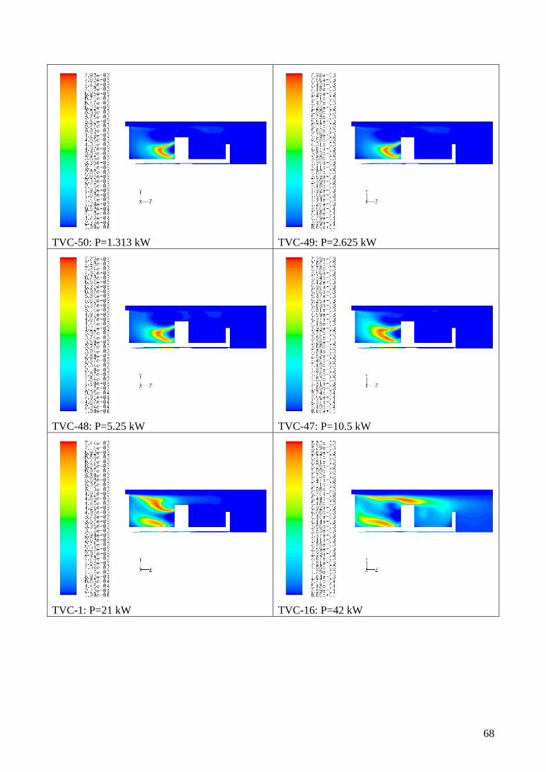
TVC-50: P=1.313 kW

TVC-49: P=2.625 kW

TVC-48: P=5.25 kW

TVC-47: P=10.5 kW

TVC-1: P=21 kW

TVC-16: P=42 kW

68

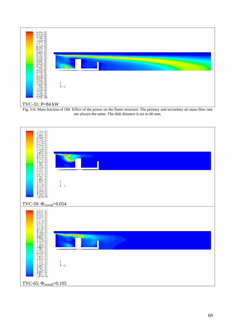
TVC-31: P=84 kW Fig. 5-6: Mass fraction of OH. Effect of the power on the flame structure. The primary and secondary air mass flow rate

are always the same. The disk distance is set to 60 mm.

TVC-59: Φoverall=0.054

TVC-65: Φoverall=0.105

69

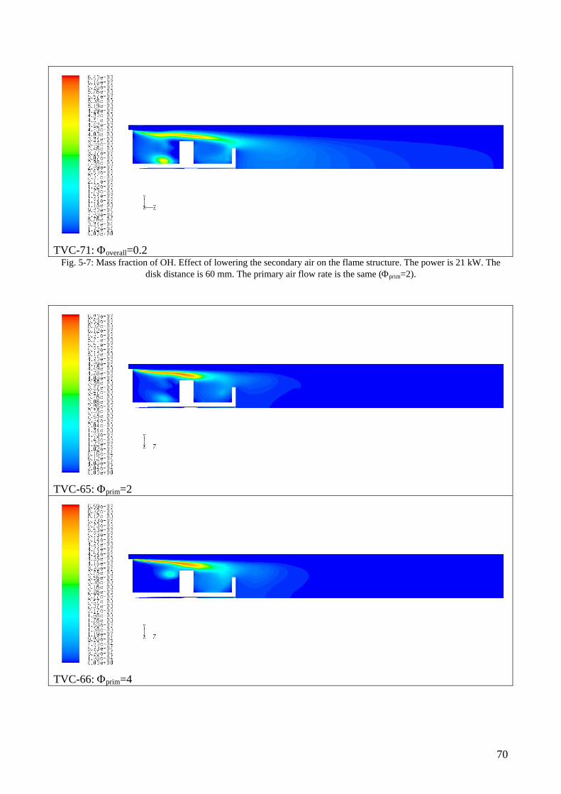
TVC-71: Φoverall=0.2 Fig. 5-7: Mass fraction of OH. Effect of lowering the secondary air on the flame structure. The power is 21 kW. The

disk distance is 60 mm. The primary air flow rate is the same (Φprim=2).

TVC-65: Φprim=2

TVC-66: Φprim=4

70

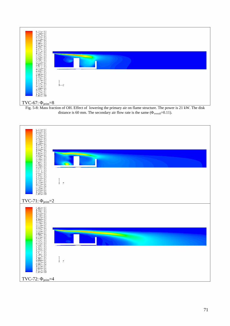
TVC-67: Φprim=8 Fig. 5-8: Mass fraction of OH. Effect of lowering the primary air on flame structure. The power is 21 kW. The disk

distance is 60 mm. The secondary air flow rate is the same (Φoverall=0.11).

TVC-71: Φprim=2

TVC-72: Φprim=4

71

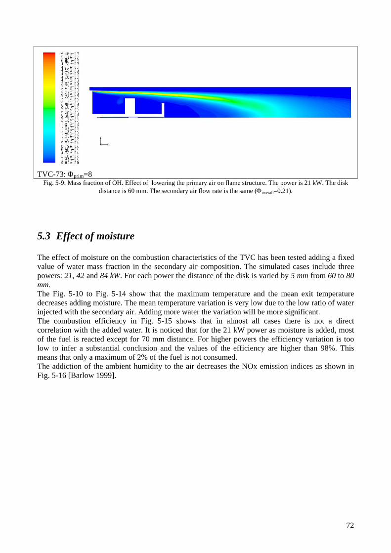
TVC-73: Φprim=8 Fig. 5-9: Mass fraction of OH. Effect of lowering the primary air on flame structure. The power is 21 kW. The disk

distance is 60 mm. The secondary air flow rate is the same (Φoverall=0.21).

5.3 Effect of moisture The effect of moisture on the combustion characteristics of the TVC has been tested adding a fixed value of water mass fraction in the secondary air composition. The simulated cases include three powers: 21, 42 and 84 kW. For each power the distance of the disk is varied by 5 mm from 60 to 80 mm. The Fig. 5-10 to Fig. 5-14 show that the maximum temperature and the mean exit temperature decreases adding moisture. The mean temperature variation is very low due to the low ratio of water injected with the secondary air. Adding more water the variation will be more significant. The combustion efficiency in Fig. 5-15 shows that in almost all cases there is not a direct correlation with the added water. It is noticed that for the 21 kW power as moisture is added, most of the fuel is reacted except for 70 mm distance. For higher powers the efficiency variation is too low to infer a substantial conclusion and the values of the efficiency are higher than 98%. This means that only a maximum of 2% of the fuel is not consumed. The addiction of the ambient humidity to the air decreases the NOx emission indices as shown in Fig. 5-16 [Barlow 1999].

72

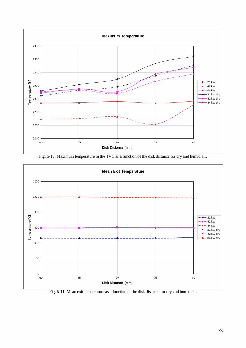
Maximum Temperature

2240

2260

2280

2300

2320

2340

2360

2380

60 65 70 75 80

Disk Distance [mm]

Tem

pera

ture

[K]

21 kW42 kW84 kW21 kW dry42 kW dry84 kW dry

Fig. 5-10: Maximum temperature in the TVC as a function of the disk distance for dry and humid air.

Mean Exit Temperature

0

200

400

600

800

1000

1200

60 65 70 75 80

Disk Distance [mm]

Tem

pera

ture

[K]

21 kW42 kW84 kW21 kW dry42 kW dry84 kW dry

Fig. 5-11: Mean exit temperature as a function of the disk distance for dry and humid air.

73

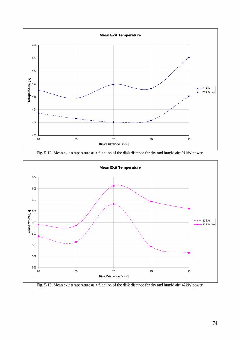
Mean Exit Temperature

460

462

464

466

468

470

472

474

60 65 70 75 80

Disk Distance [mm]

Tem

pera

ture

[K]

21 kW21 kW dry

Fig. 5-12: Mean exit temperature as a function of the disk distance for dry and humid air: 21kW power.

Mean Exit Temperature

596

597

598

599

600

601

602

603

604

60 65 70 75 80

Disk Distance [mm]

Tem

pera

ture

[K]

42 kW42 kW dry

Fig. 5-13: Mean exit temperature as a function of the disk distance for dry and humid air: 42kW power.

74

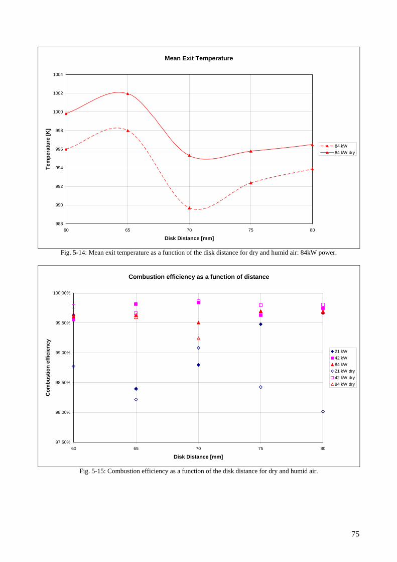
Mean Exit Temperature

988

990

992

994

996

998

1000

1002

1004

60 65 70 75 80

Disk Distance [mm]

Tem

pera

ture

[K]

84 kW84 kW dry

Fig. 5-14: Mean exit temperature as a function of the disk distance for dry and humid air: 84kW power.

Combustion efficiency as a function of distance

97.50%

98.00%

98.50%

99.00%

99.50%

100.00%

60 65 70 75 80

Disk Distance [mm]

Com

bust

ion

effic

ienc

y

21 kW42 kW84 kW21 kW dry42 kW dry84 kW dry

Fig. 5-15: Combustion efficiency as a function of the disk distance for dry and humid air.

75

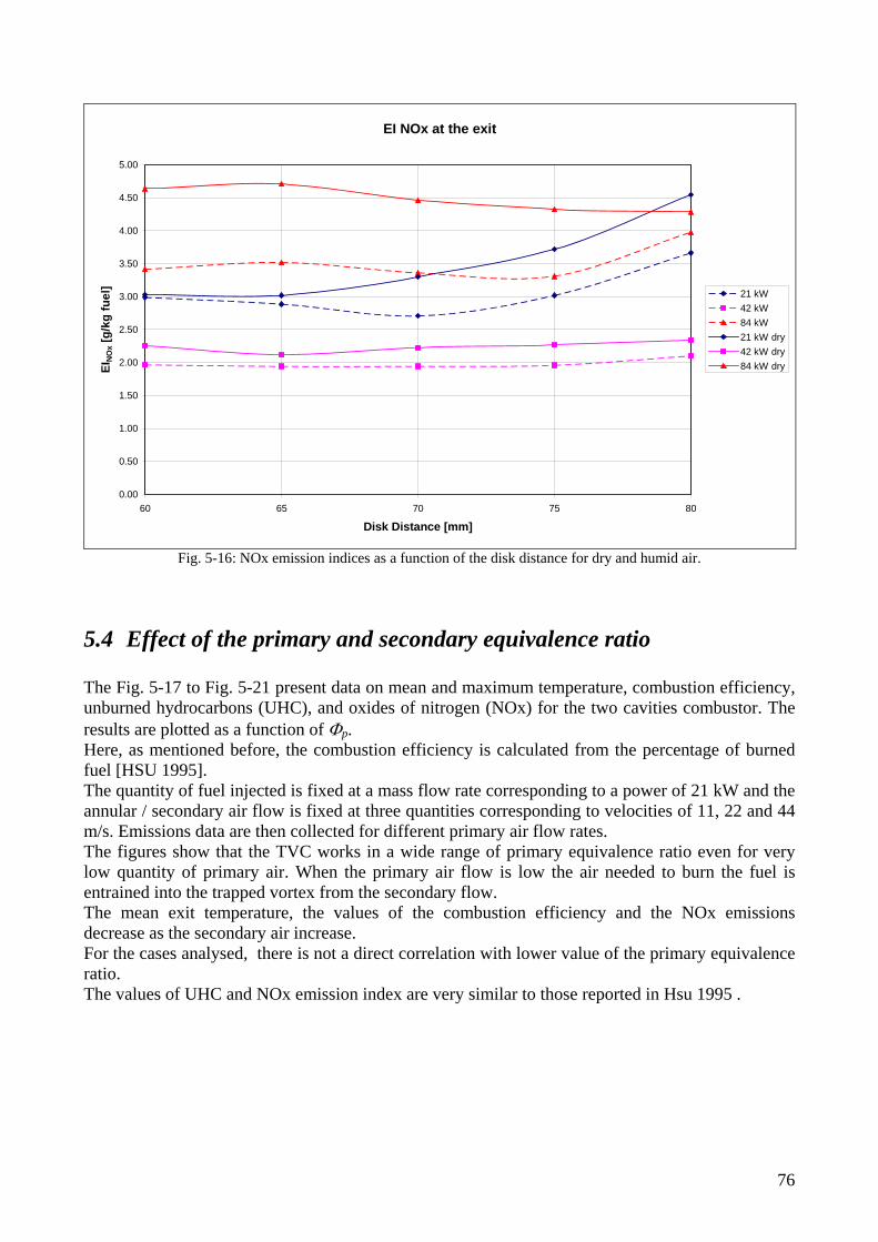
EI NOx at the exit

0.00

0.50

1.00

1.50

2.00

2.50

3.00

3.50

4.00

4.50

5.00

60 65 70 75 80

Disk Distance [mm]

EIN

Ox [

g/kg

fuel

]

21 kW42 kW84 kW21 kW dry42 kW dry84 kW dry

Fig. 5-16: NOx emission indices as a function of the disk distance for dry and humid air.

5.4 Effect of the primary and secondary equivalence ratio The Fig. 5-17 to Fig. 5-21 present data on mean and maximum temperature, combustion efficiency, unburned hydrocarbons (UHC), and oxides of nitrogen (NOx) for the two cavities combustor. The results are plotted as a function of Φp. Here, as mentioned before, the combustion efficiency is calculated from the percentage of burned fuel [HSU 1995]. The quantity of fuel injected is fixed at a mass flow rate corresponding to a power of 21 kW and the annular / secondary air flow is fixed at three quantities corresponding to velocities of 11, 22 and 44 m/s. Emissions data are then collected for different primary air flow rates. The figures show that the TVC works in a wide range of primary equivalence ratio even for very low quantity of primary air. When the primary air flow is low the air needed to burn the fuel is entrained into the trapped vortex from the secondary flow. The mean exit temperature, the values of the combustion efficiency and the NOx emissions decrease as the secondary air increase. For the cases analysed, there is not a direct correlation with lower value of the primary equivalence ratio. The values of UHC and NOx emission index are very similar to those reported in Hsu 1995 .

76

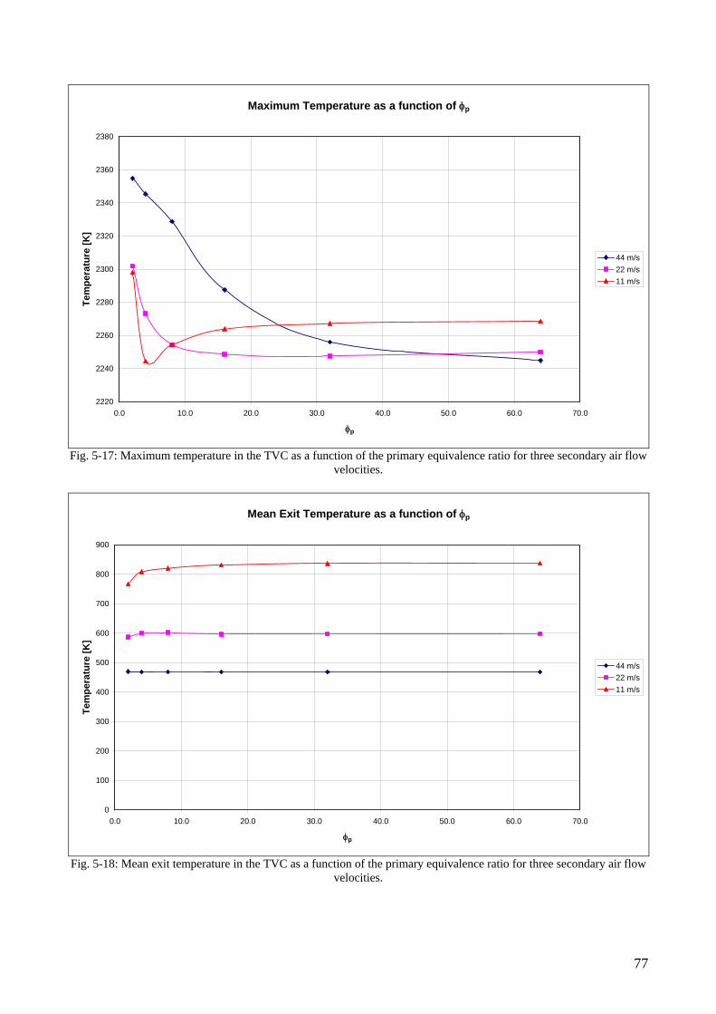
Maximum Temperature as a function of φp

2220

2240

2260

2280

2300

2320

2340

2360

2380

0.0 10.0 20.0 30.0 40.0 50.0 60.0 70.0

φp

Tem

pera

ture

[K]

44 m/s22 m/s11 m/s

Fig. 5-17: Maximum temperature in the TVC as a function of the primary equivalence ratio for three secondary air flow

velocities.

Mean Exit Temperature as a function of φp

0

100

200

300

400

500

600

700

800

900

0.0 10.0 20.0 30.0 40.0 50.0 60.0 70.0

φp

Tem

pera

ture

[K]

44 m/s22 m/s11 m/s

Fig. 5-18: Mean exit temperature in the TVC as a function of the primary equivalence ratio for three secondary air flow

velocities.

77

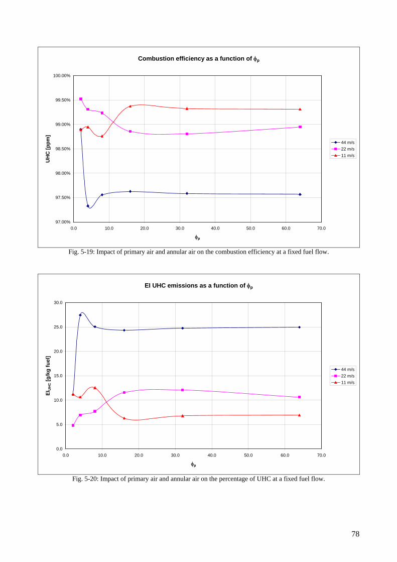
Combustion efficiency as a function of φp

97.00%

97.50%

98.00%

98.50%

99.00%

99.50%

100.00%

0.0 10.0 20.0 30.0 40.0 50.0 60.0 70.0

φp

UH

C [p

pm]

44 m/s22 m/s11 m/s

Fig. 5-19: Impact of primary air and annular air on the combustion efficiency at a fixed fuel flow.

EI UHC emissions as a function of φp

0.0

5.0

10.0

15.0

20.0

25.0

30.0

0.0 10.0 20.0 30.0 40.0 50.0 60.0 70.0

φp

EIU

HC [g

/kg

fuel

]

44 m/s22 m/s11 m/s

Fig. 5-20: Impact of primary air and annular air on the percentage of UHC at a fixed fuel flow.

78

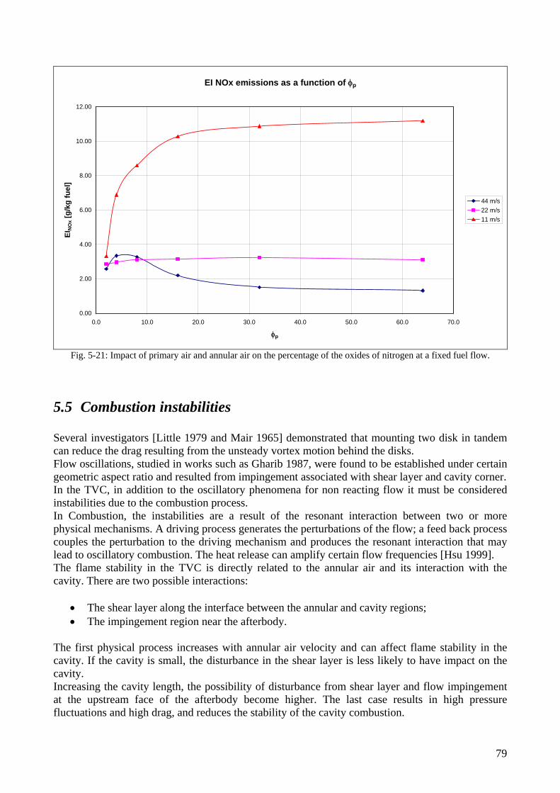
EI NOx emissions as a function of φp

0.00

2.00

4.00

6.00

8.00

10.00

12.00

0.0 10.0 20.0 30.0 40.0 50.0 60.0 70.0

φp

EIN

Ox [

g/kg

fuel

]

44 m/s22 m/s11 m/s

Fig. 5-21: Impact of primary air and annular air on the percentage of the oxides of nitrogen at a fixed fuel flow.

5.5 Combustion instabilities Several investigators [Little 1979 and Mair 1965] demonstrated that mounting two disk in tandem can reduce the drag resulting from the unsteady vortex motion behind the disks. Flow oscillations, studied in works such as Gharib 1987, were found to be established under certain geometric aspect ratio and resulted from impingement associated with shear layer and cavity corner. In the TVC, in addition to the oscillatory phenomena for non reacting flow it must be considered instabilities due to the combustion process. In Combustion, the instabilities are a result of the resonant interaction between two or more physical mechanisms. A driving process generates the perturbations of the flow; a feed back process couples the perturbation to the driving mechanism and produces the resonant interaction that may lead to oscillatory combustion. The heat release can amplify certain flow frequencies [Hsu 1999]. The flame stability in the TVC is directly related to the annular air and its interaction with the cavity. There are two possible interactions:

• The shear layer along the interface between the annular and cavity regions; • The impingement region near the afterbody.

The first physical process increases with annular air velocity and can affect flame stability in the cavity. If the cavity is small, the disturbance in the shear layer is less likely to have impact on the cavity. Increasing the cavity length, the possibility of disturbance from shear layer and flow impingement at the upstream face of the afterbody become higher. The last case results in high pressure fluctuations and high drag, and reduces the stability of the cavity combustion.

79

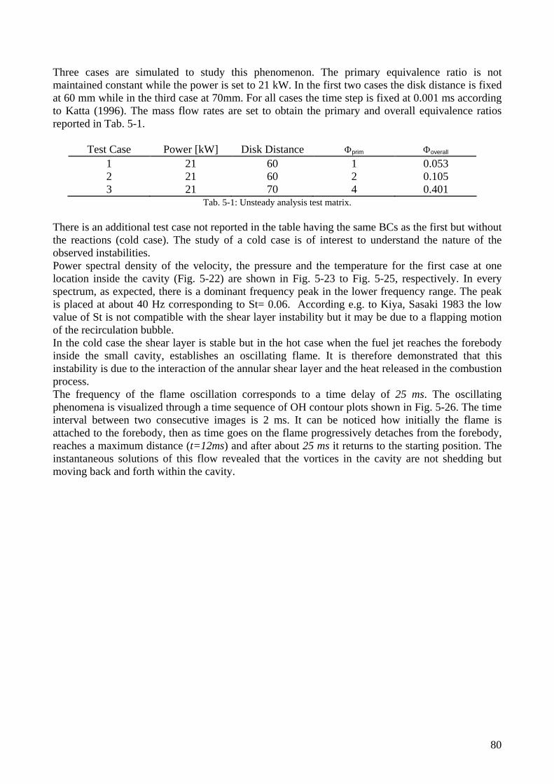
Three cases are simulated to study this phenomenon. The primary equivalence ratio is not maintained constant while the power is set to 21 kW. In the first two cases the disk distance is fixed at 60 mm while in the third case at 70mm. For all cases the time step is fixed at 0.001 ms according to Katta (1996). The mass flow rates are set to obtain the primary and overall equivalence ratios reported in Tab. 5-1.

Test Case Power [kW] Disk Distance Φprim Φoverall

1 21 60 1 0.053 2 21 60 2 0.105 3 21 70 4 0.401

Tab. 5-1: Unsteady analysis test matrix. There is an additional test case not reported in the table having the same BCs as the first but without the reactions (cold case). The study of a cold case is of interest to understand the nature of the observed instabilities. Power spectral density of the velocity, the pressure and the temperature for the first case at one location inside the cavity (Fig. 5-22) are shown in Fig. 5-23 to Fig. 5-25, respectively. In every spectrum, as expected, there is a dominant frequency peak in the lower frequency range. The peak is placed at about 40 Hz corresponding to St= 0.06. According e.g. to Kiya, Sasaki 1983 the low value of St is not compatible with the shear layer instability but it may be due to a flapping motion of the recirculation bubble. In the cold case the shear layer is stable but in the hot case when the fuel jet reaches the forebody inside the small cavity, establishes an oscillating flame. It is therefore demonstrated that this instability is due to the interaction of the annular shear layer and the heat released in the combustion process. The frequency of the flame oscillation corresponds to a time delay of 25 ms. The oscillating phenomena is visualized through a time sequence of OH contour plots shown in Fig. 5-26. The time interval between two consecutive images is 2 ms. It can be noticed how initially the flame is attached to the forebody, then as time goes on the flame progressively detaches from the forebody, reaches a maximum distance (t=12ms) and after about 25 ms it returns to the starting position. The instantaneous solutions of this flow revealed that the vortices in the cavity are not shedding but moving back and forth within the cavity.

80

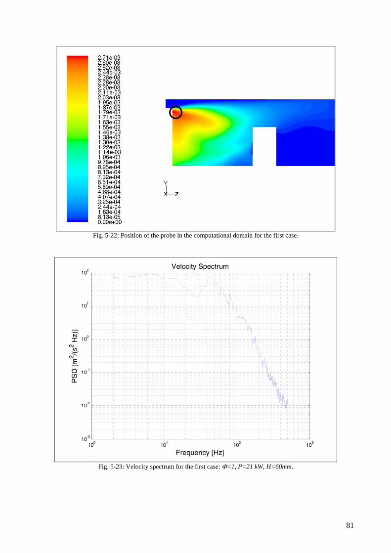
Fig. 5-22: Position of the probe in the computational domain for the first case.

100

101

102

103

10-3

10-2

10-1

100

101

102

Velocity Spectrum

Frequency [Hz]

PS

D [m

2 /(s2 H

z)]

Fig. 5-23: Velocity spectrum for the first case: Φ=1, P=21 kW, H=60mm.

81

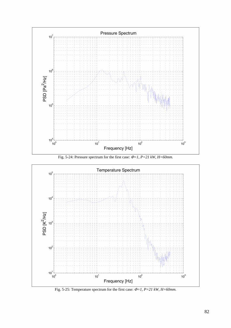
100

101

102

103

104

105

106

107

Pressure Spectrum

Frequency [Hz]

PS

D [P

a2 /Hz]

Fig. 5-24: Pressure spectrum for the first case: Φ=1, P=21 kW, H=60mm.

100

101

102

103

101

102

103

104

105

Temperature Spectrum

PS

D [K

2 /Hz]

Frequency [Hz]

Fig. 5-25: Temperature spectrum for the first case: Φ=1, P=21 kW, H=60mm.

82

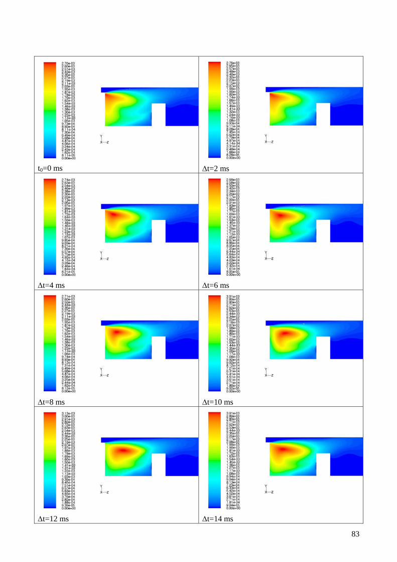
t0=0 ms Δt=2 ms

Δt=4 ms Δt=6 ms

Δt=8 ms Δt=10 ms

Δt=12 ms Δt=14 ms

83

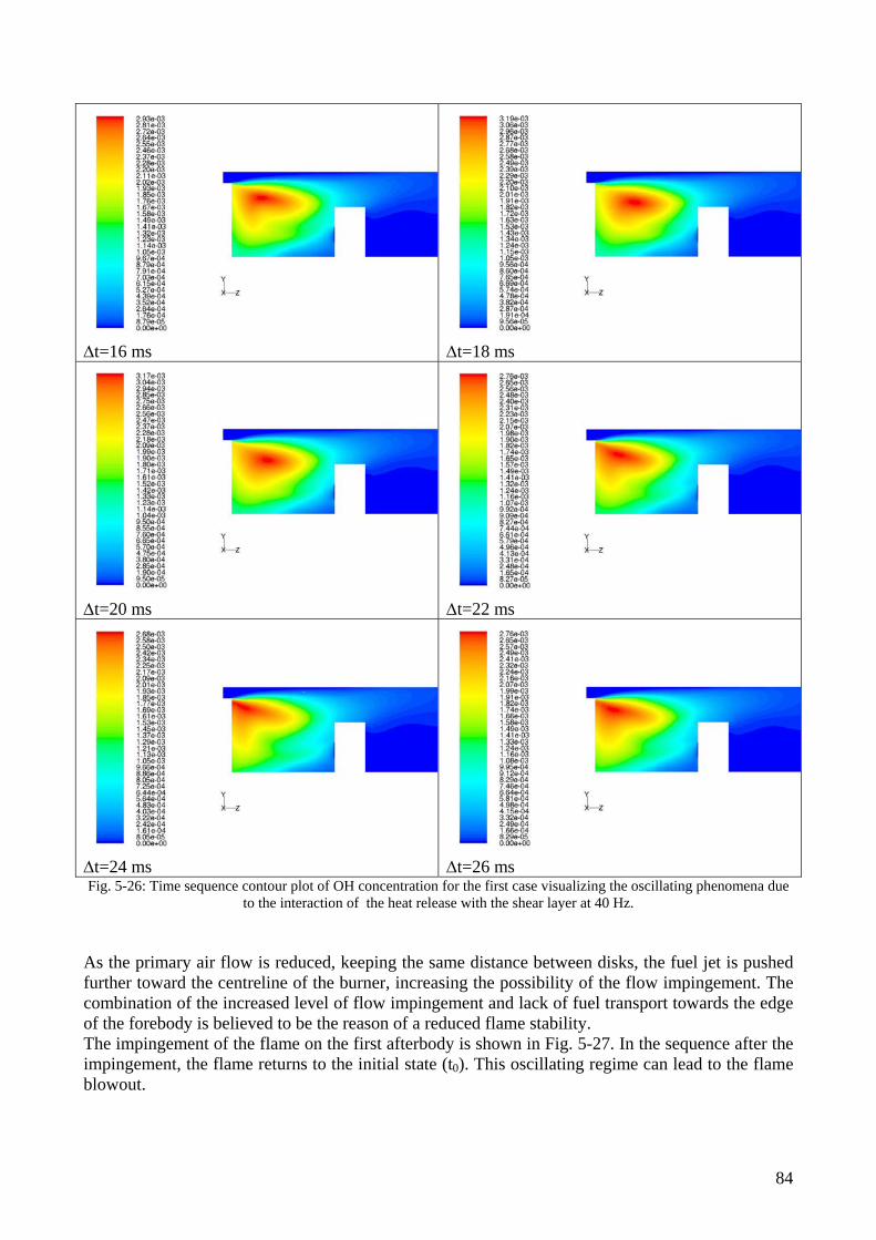
Δt=16 ms Δt=18 ms

Δt=20 ms Δt=22 ms

Δt=24 ms Δt=26 ms Fig. 5-26: Time sequence contour plot of OH concentration for the first case visualizing the oscillating phenomena due

to the interaction of the heat release with the shear layer at 40 Hz. As the primary air flow is reduced, keeping the same distance between disks, the fuel jet is pushed further toward the centreline of the burner, increasing the possibility of the flow impingement. The combination of the increased level of flow impingement and lack of fuel transport towards the edge of the forebody is believed to be the reason of a reduced flame stability. The impingement of the flame on the first afterbody is shown in Fig. 5-27. In the sequence after the impingement, the flame returns to the initial state (t0). This oscillating regime can lead to the flame blowout.

84

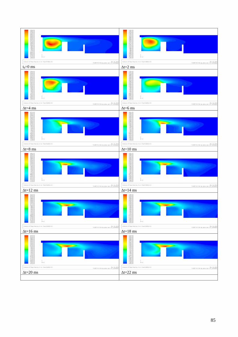
t0=0 ms Δt=2 ms

Δt=4 ms Δt=6 ms

Δt=8 ms Δt=10 ms

Δt=12 ms Δt=14 ms

Δt=16 ms Δt=18 ms

Δt=20 ms Δt=22 ms

85

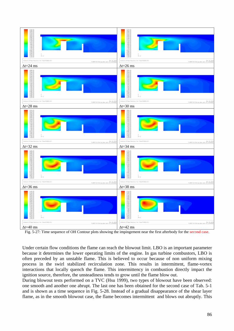
Δt=24 ms Δt=26 ms

Δt=28 ms Δt=30 ms

Δt=32 ms Δt=34 ms

Δt=36 ms Δt=38 ms

Δt=40 ms Δt=42 ms Fig. 5-27: Time sequence of OH Contour plots showing the impingement near the first afterbody for the second case.

Under certain flow conditions the flame can reach the blowout limit. LBO is an important parameter because it determines the lower operating limits of the engine. In gas turbine combustors, LBO is often preceded by an unstable flame. This is believed to occur because of non uniform mixing process in the swirl stabilized recirculation zone. This results in intermittent, flame-vortex interactions that locally quench the flame. This intermittency in combustion directly impact the ignition source, therefore, the unsteadiness tends to grow until the flame blow out. During blowout tests performed on a TVC (Hsu 1999), two types of blowout have been observed: one smooth and another one abrupt. The last one has been obtained for the second case of Tab. 5-1 and is shown as a time sequence in Fig. 5-28. Instead of a gradual disappearance of the shear layer flame, as in the smooth blowout case, the flame becomes intermittent and blows out abruptly. This

86

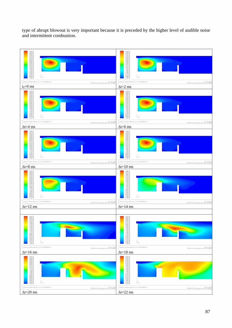
type of abrupt blowout is very important because it is preceded by the higher level of audible noise and intermittent combustion.

t0=0 ms Δt=2 ms

Δt=4 ms Δt=6 ms

Δt=8 ms Δt=10 ms

Δt=12 ms Δt=14 ms

Δt=16 ms Δt=18 ms

Δt=20 ms Δt=22 ms

87

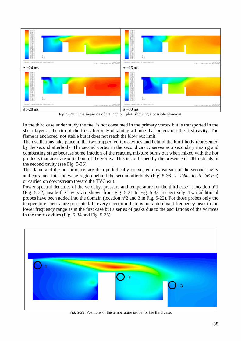
Δt=24 ms Δt=26 ms

Δt=28 ms Δt=30 ms Fig. 5-28: Time sequence of OH contour plots showing a possible blow-out.

In the third case under study the fuel is not consumed in the primary vortex but is transported in the shear layer at the rim of the first afterbody obtaining a flame that bulges out the first cavity. The flame is anchored, not stable but it does not reach the blow out limit. The oscillations take place in the two trapped vortex cavities and behind the bluff body represented by the second afterbody. The second vortex in the second cavity serves as a secondary mixing and combusting stage because some fraction of the reacting mixture burns out when mixed with the hot products that are transported out of the vortex. This is confirmed by the presence of OH radicals in the second cavity (see Fig. 5-36). The flame and the hot products are then periodically convected downstream of the second cavity and entrained into the wake region behind the second afterbody (Fig. 5-36 Δt=24ms to Δt=36 ms) or carried on downstream toward the TVC exit. Power spectral densities of the velocity, pressure and temperature for the third case at location n°1 (Fig. 5-22) inside the cavity are shown from Fig. 5-31 to Fig. 5-33, respectively. Two additional probes have been added into the domain (location n°2 and 3 in Fig. 5-22). For those probes only the temperature spectra are presented. In every spectrum there is not a dominant frequency peak in the lower frequency range as in the first case but a series of peaks due to the oscillations of the vortices in the three cavities (Fig. 5-34 and Fig. 5-35).

1

2

3

Fig. 5-29: Positions of the temperature probe for the third case.

88

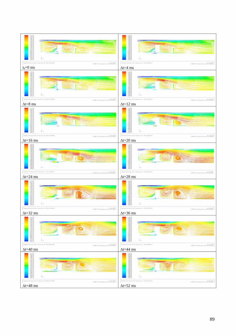
t0=0 ms Δt=4 ms

Δt=8 ms Δt=12 ms

Δt=16 ms Δt=20 ms

Δt=24 ms Δt=28 ms

Δt=32 ms Δt=36 ms

Δt=40 ms Δt=44 ms

Δt=48 ms Δt=52 ms

89

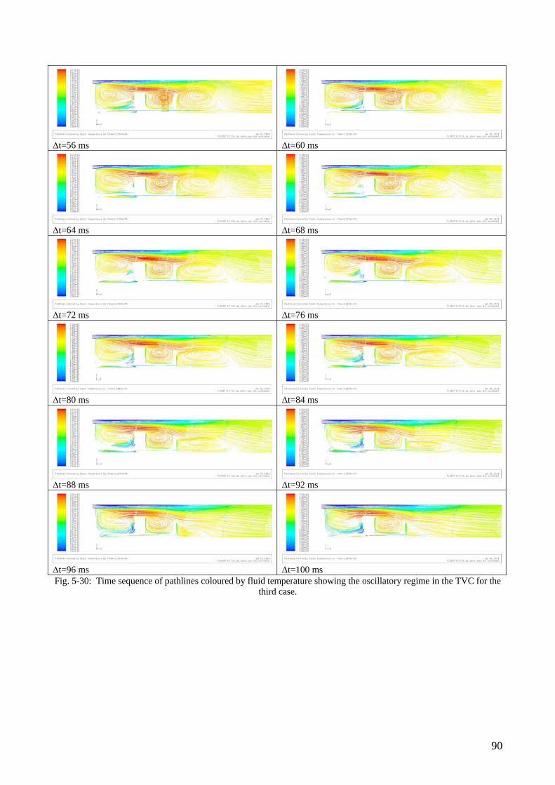
Δt=56 ms Δt=60 ms

Δt=64 ms Δt=68 ms

Δt=72 ms Δt=76 ms

Δt=80 ms Δt=84 ms

Δt=88 ms Δt=92 ms

Δt=96 ms Δt=100 ms Fig. 5-30: Time sequence of pathlines coloured by fluid temperature showing the oscillatory regime in the TVC for the

third case.

90

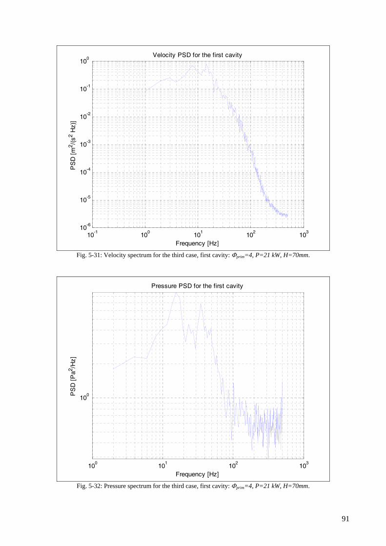
10-1

100

101

102

103

10-6

10-5

10-4

10-3

10-2

10-1

100

Frequency [Hz]

PS

D [

m2 /(

s2 Hz)

]

Velocity PSD for the first cavity

Fig. 5-31: Velocity spectrum for the third case, first cavity: Φprim=4, P=21 kW, H=70mm.

100

101

102

103

100

Frequency [Hz]

PS

D [

Pa2 /H

z]

Pressure PSD for the first cavity

Fig. 5-32: Pressure spectrum for the third case, first cavity: Φprim=4, P=21 kW, H=70mm.

91

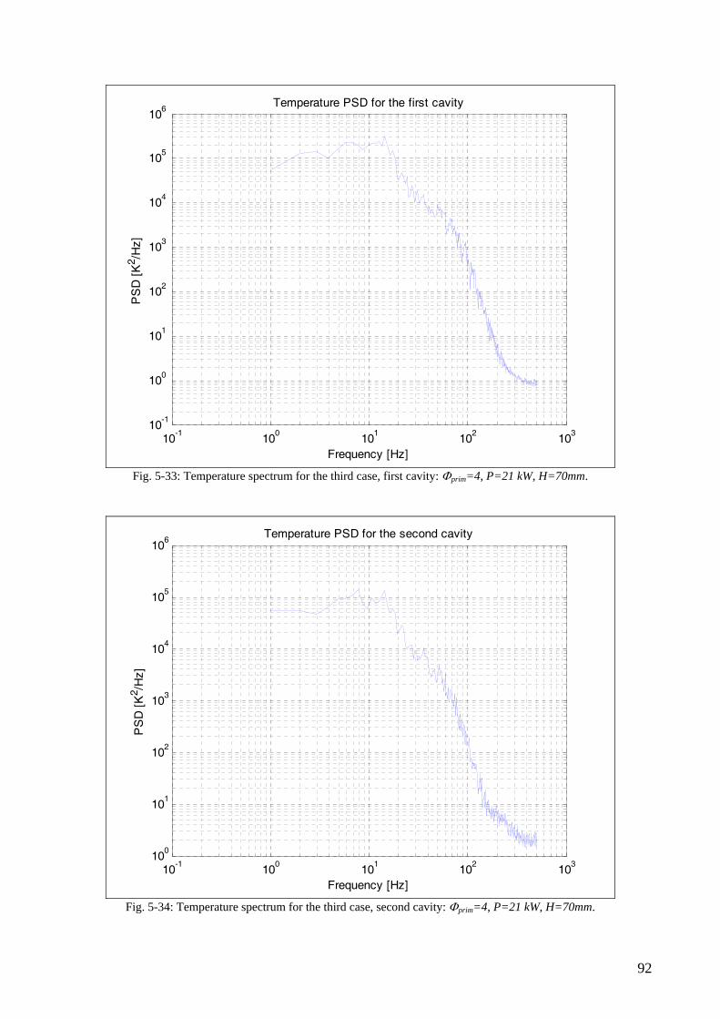
10-1

100

101

102

103

10-1

100

101

102

103

104

105

106

Frequency [Hz]

PS

D [

K2 /H

z]

Temperature PSD for the first cavity

Fig. 5-33: Temperature spectrum for the third case, first cavity: Φprim=4, P=21 kW, H=70mm.

10-1

100

101

102

103

100

101

102

103

104

105

106

Frequency [Hz]

PS

D [

K2 /H

z]

Temperature PSD for the second cavity

Fig. 5-34: Temperature spectrum for the third case, second cavity: Φprim=4, P=21 kW, H=70mm.

92

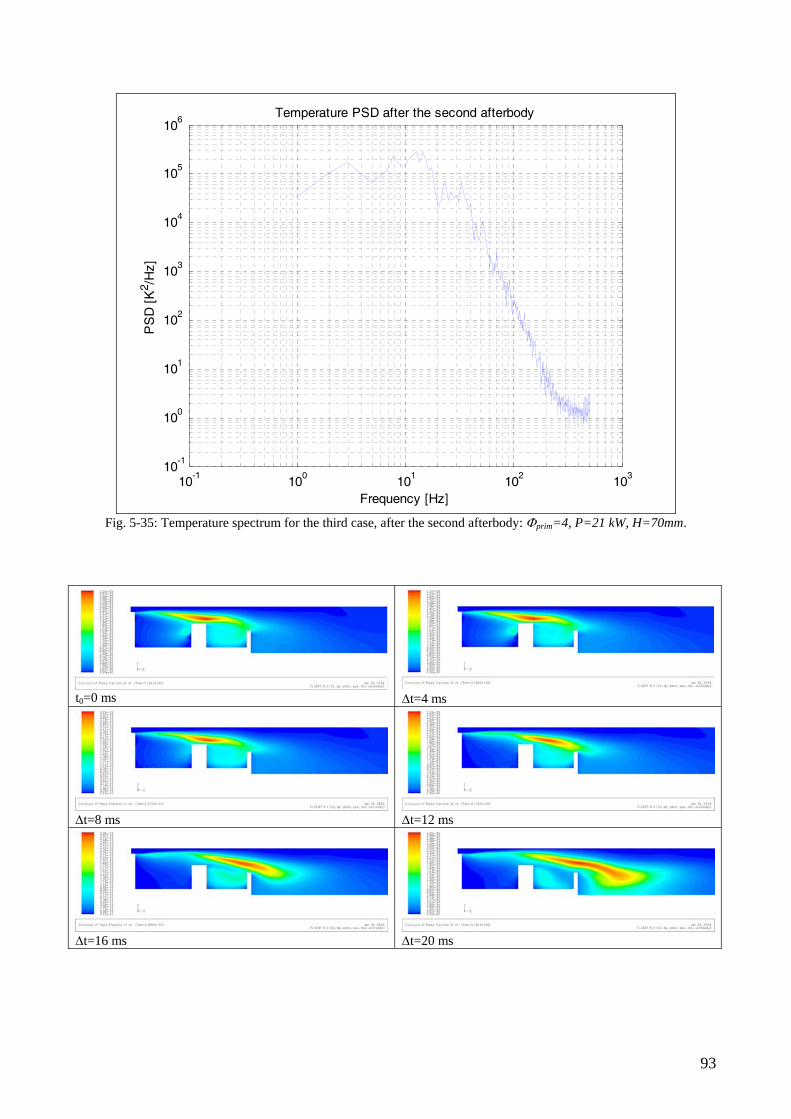
10-1

100

101

102

103

10-1

100

101

102

103

104

105

106

Frequency [Hz]

PS

D [

K2 /H

z]

Temperature PSD after the second afterbody

Fig. 5-35: Temperature spectrum for the third case, after the second afterbody: Φprim=4, P=21 kW, H=70mm.

t0=0 ms Δt=4 ms

Δt=8 ms Δt=12 ms

Δt=16 ms Δt=20 ms

93

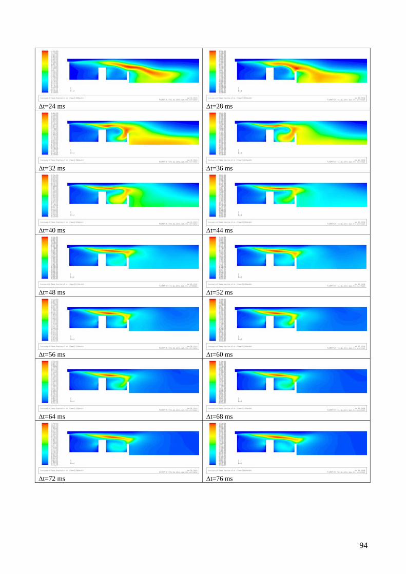
Δt=24 ms Δt=28 ms

Δt=32 ms Δt=36 ms

Δt=40 ms Δt=44 ms

Δt=48 ms Δt=52 ms

Δt=56 ms Δt=60 ms

Δt=64 ms Δt=68 ms

Δt=72 ms Δt=76 ms

94

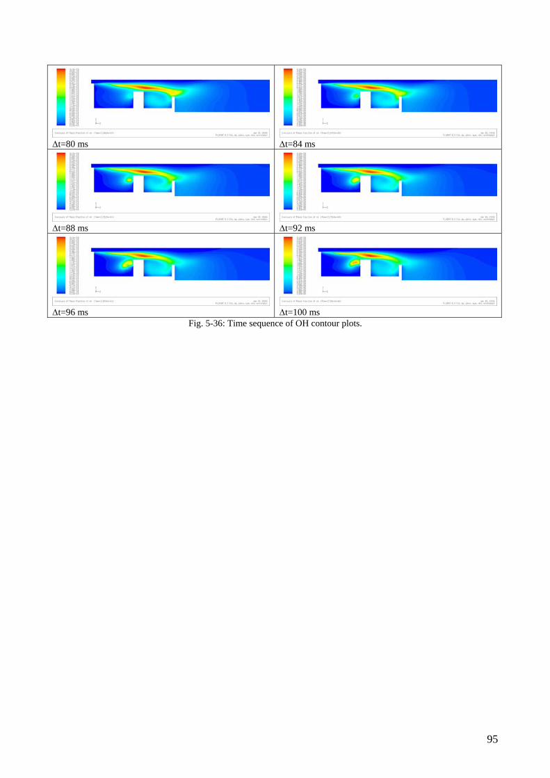
Δt=80 ms Δt=84 ms

Δt=88 ms Δt=92 ms

Δt=96 ms Δt=100 ms Fig. 5-36: Time sequence of OH contour plots.

95

6 Conclusions and future perspectives The performances and the stability of the ENEA TVC has been numerically investigated. The geometry is based on the one proposed by Hsu 1995. In this kind of combustor two cavities are sized to trap vortices when air flow passes through. Fuel and primary air are injected directly into the vortex from multiple jets in the down stream wall of the first cavity. The underlying idea of the TVC is that the flame, once established in the trapped vortex, should remain stable over a wide range of operating conditions. This idea is assessed in the present work and the main parameters - power, distance of the first cavity disks, primary and secondary equivalence ratios and humidity - are examined for several test cases. The TVC performances have been detailed in terms of NOx, UHC, and combustion efficiency trend as a function of the listed parameters. The TVC stability have been tested for three cases and results shown as time sequences of OH contour plots or temperature pathlines. Furthermore the spectra obtained from some sample probes, located in strategic points of the computational domain, have been analyzed in order to characterize the dynamic behaviour. The 3D-CFD simulations depict several distinct vortices in the TVC cavities. In the all analysed cases three main vortices develop: two in the first and second cavity and one behind the last disk as an effect of the shear layer. In the first cavity arise a secondary vortex, mainly because of the interaction between fuel and air jets injected in the cavity, and a third vortex, due to the motion of the mixture flow. Depending on the quantity of primary or secondary air mass flow rate, the dimension of the main vortex in the first cavity can change. This vortex is responsible of the air-fuel-hot product mixing. For reduced dimensions the amount of re-ingested hot products is low. Best results are obtained when the vortex spreads over the entire cavity. For what concern the flame front, it depends on the various regimes established in the combustor. Depending on the power and on the primary and secondary air flow rate, the flame can be confined in the first cavity or bulged out radially toward the annular air, reaching the second cavity or passing the second afterbody. When the flame is confined in the first cavity, the primary zone may not be affected by entrainment of cold annular air. The higher temperatures at this condition result in good combustion efficiency, but higher NOx. The effect of moisture on the combustion has been tested adding a fixed value of water mass fraction in the secondary air composition. Results do not show a direct correlation between combustion efficiency and added water, while lower NOx emission indices has been obtained by adding ambient humidity. For future development it could be useful to inject water directly into the combustion airstream, a technique commonly used in gas turbine combustion to enhance efficiency and decrease emissions at lower costs. The TVC works in a wide range of primary and secondary equivalence ratios, reaching overall values below common limits for gas turbine combustors. Results obtained increasing the secondary air flow show the decrease of the mean exit temperature, of the combustion efficiency value and of the NOx emissions. It is noticed that in all the analysed cases the value of the efficiency is always higher than 97%. This means that only a maximum of 3% of the fuel is not consumed. Another TVC feature studied is the combustion instability. Two kind of instabilities have been detected, both directly related to the annular air and its interaction with the cavity. The first is due to the interaction of the shear layer along the interface between the annular and cavity regions, while the impingement region near the afterbody causes the second one. Referring to the first instability, the instantaneous solutions have revealed that the vortices in the cavity are not shedding, but moving back and forth within the cavity. The spectra show a peak corresponding to St=0.06, a low value due to a flapping motion of the recirculation bubble. As the

96

primary air flow is reduced, keeping the same distance between disks, the fuel jet is pushed further toward the centreline of the burner, thus increasing the possibility of the flow impingement and initializing the second kind of instability. This oscillating regime can lead to the flame blowout. Increasing the distance between the disk and maintaining a low primary flow rate (primary equivalence ratio of about 4), the flame resulted anchored but not stable. The oscillations take place in the trapped vortex cavities and behind the second afterbody. In every spectrum obtained from some probes, opportunely placed in the domain, there is not a dominant frequency peak in the lower frequency range, but a series of peaks, mostly because the vortices oscillations due to the combustion take place in the three cavities. In conclusion, the ENEA TVC offers a wide range of operating conditions with reasonable combustion efficiency and low emissions in a simple and compact combustor. However, further work is required. For future study, Large Eddy Simulation (LES) will be utilized in the numerical code to predict smaller scale structures and quantities fluctuations. More working conditions should be examined to better understand the dynamic behaviour of the TVC and to evaluate methods for maintaining good performance characteristics while substantially reducing NOx.

97

References Books: [1a] Çengel Y.A. – Introduction to Thermodynamics and Heat Transfer – McGraw Hill Series in

Mechanical Engineering, 1997; [2a] Chigier N. – Combustion Measurements – Hemisphere Publishing Corporation 1991; [3a] Chigier N., Beér J. M. – Combustion Aerodynamics – Applied Science Publishers LTD

1972; [4a] Chomiak J. – Combustion: a study in Theory, Fact and Application – Abacus Press NY

1990; [5a] Fluent Handbook; [6a] Gaydon A.G., Wolfhard H.G. – Flames: their Structure, Radiation and Temperature –

Chapman & Hall LTD London 1960; [7a] Glassman I. – Combustion, Third Ed. – Academic Press 1996; [8a] Kuo Kennet K. – Principles of Combustion – John Wiley and Sons 1986; [9a] Laufer G. – Introduction to Optics and Laser in Engineering – Cambridge University Press

1996; [10a] Lefebvre Arthur H. – Gas Turbine Combustion – Taylor & Francis 1983; [11a] Mellor A. M. – Design of modern Turbine Combustors –Academic Press 1990; [12a] Peters N., and Rogg B., - Reduced Kinetic Mechanisms for Applications in Combustion

Systems - Springer-Verlag Berlin 1993; [13a] Poinsot T., Veynante D. – Theoretical and Numerical Combustion – Edwards 2005; [14a] Pope S. B. – Turbulent Flows – Cambridge University Press 2000; [15a] Raffel M., Willert C., Kompenhans J. – Particle Image Velocimetry – Springer-Verlag

Berlin 1998; [16a] Sabetta F. – Gasdinamica – Edizioni Ingegneria 2000 1999; [17a] Smoke M.D. – Reduced Kinetic Mechanisms and Asymptotic Approximations for Methane-

Air Flames – Lecture Notes in Physics, Springer-Verlag Berlin 1991; [18a] Stella A. – Experimental Investigation of Turbulent Premixed Combusting Flows – Phd

Thesis 2001; [19a] Tavoularis S. – Measurement in Fluid Mechanics – Cambridge University Press 2005; [20a] Turns Stephen R. – Introduction to Combustion – McGraw-Hill Publ. Co. 2000; [21a] Warnatz T.Z., Maas U., Dibble R.W. – Combustion – Springer-Verlag. Berlin 1996; [22a] Williams Forman A. – Combustion Theory 2th Edition – Perseus Books Publishing 1985; Articles: [1b] Barlow, R. S., Smith, N. S. A., Chen, J.-Y., and Bilger, R. W. – Nitric Oxide Formation in

Dilute Hydrogen Jet Flames: Isolation of the Effects of Radiation and Turbulence-Chemistry Submodels – Combust. Flame 117:4-31 (1999);

[2b] Bruno C., Losurdo M. – The Trapped Vortex Combustor: and advanced combustion technology for aerospace and gas turbine applications – Advanced Combustion and Aerothermal Technologies, 365-384 (2007);

[3b] Bucher J., Edmonds R.G., Steele R.C., Kendrick D.W., Chenevert B.C., and Malte P.C., – The Development of a Lean-Premixed Trapped Vortex Combustor – ASME Paper #GT2003-38236;

[4b] Burrus D.L., Johnson A.W., Roquemore W.M., and Shouse D.T., “Performance – Assessment of a Prototype Trapped Vortex Combustor Concept for Gas Turbine Application – ASME Paper # 2001-GT-0087;

98

[5b] Frenklach, M., Wang, H., and Rabinowitz, M. J., – Optimization and Analysis of Large Chemical Kinetic Mechanisms Using the Solution Mapping Method. Combustion of Methane – Progress in Energy and Combustion Science, 18: 47-73 (1992);

[6b] Gharib, M. and Roshko, A., 1987 – The Effect of Flow Oscillations on Cavity Drag,” Journal of Fluid Mechanics – 177, pp. 501-530;

[7b] Hsu K.-Y.. Carter C.D., Katta V.R., and Roquemore W.M. – Characteristics of combustion instability associated with trapped-vortex burner - AIAA Paper 99-0488, 37rd Aerospace Science Meeting and Exhibit, January 11-14, 1999, Reno, NV;

[8b] Hsu K.-Y., Goss L.P., Trump D.D., and Roquemore W.M. – Performance of a Trapped Vortex Combustor – AIAA Paper 95-0810, 33rd Aerospace Science Meeting and Exhibit, January 9-12, 1995, Reno, NV;

[9b] Kalin M. – Overview of the ALM TVC Combustor – private communication with CEO of ALM Turbine, June, 2005;

[10b] Katta V.R., Roquemore W.M. – Numerical Studies on Trapped-Vortex Combustor – AIAA Paper 96-2660, 32nd AIAA/ASME/SAE/ASEE Joint Propulsion Conference, July 1-3 1996, Lake Buena Vista, FL;

[11b] Katta V.R., and Roquemore W.M. – Study on a Trapped-Vortex Combustor – Effect of Injection on Flow Dynamicas – Journal of Propulsion and Power, Vol. 14, No. 3, May-June 1998;

[12b] Kurimoto N., Suzuki Y., Kasagi N. – Active control of lifted diffusion flames with arrayed micro actuators – Exp. In Fluids (2005) 39: 995-1008;

[13b] Little Jr. B.H. and Whipkey R.R. – Locked vortex afterbodies – presented as paper 78-1179 at the AIAA 11th Fluid and Plasma Dynamics Conference, Seattle, Wash., July 10-12, 1978;

[14b] Magnussen B.F. – On the structure of turbulence and a generalized Eddy Dissipation Concept for chemical reaction in turbulent flow – 19th AIAA Aerospace Science meeting, Missouri, Jan 12-15, 1981;

[15b] Mair W.A. – The effect of a Rear-Mounted Disc on the Drag of a Blunt Based body of revolution – The Aeronautical quarterly 1965 (16), 350-360;

[16b] Meyer T.R., Brown M.S., Fonov S., Goss L.P., Gord J.R., Shouse D.T., Belovich V.M., Roquemore W.M., Cooper C.S., Kim E.S., and Haynes J.M. – Optical Diagnostics and Numerical Characterization of a Trapped-Vortex Combustor – 38th AIAA/ASME/SAE/ASEE Joint Propulsion Conference & Exhibit, 7-10 July 2002, Indianapolis, Indiana;

[17b] Pope S. B. – Pdf Methods for Turbulent Reactive Flows – Prog. Energy Comb. Sci. 11: 119-92;

[18b] Pope S. B. – Lagrangian Pdf Methods for Turbulent Flows – Ann. Rev. Fluid Mech. 26: 23-63;

[19b] Pope S. B. – The Velocity-Dissipation Pdf Model for Turbulent Flows – Phys. Flu. A2: 1437-1449;

[20b] Pope S. B. – Turbulent Premixed Flames – Ann. Rev. of Fluid Mech. 19: 237-270; [21b] Roquemore W.M., Shouse D., Burrus D., Johnson A., Cooper C., Duncan B., Hsu K.-Y.,

Katta V.R., Sturgess G.J., and Vihinen I. – Trapped Vortex Combustor Concept for Gas Turbine Engines – AIAA Paper 2001-0483, 39th AIAA Aerospace Sciences Meeting & Exhibit, 8-11 January 2001, Reno, NV;

[22b] Straub D.L., Sidwell T.G., Maloney D. J., Casleton K.H., Richards G.A., Rogers W.A., and Golden G.M., – Simulations of a Rich Quench Lean (RQL) Trapped Vortex Combustor – presented at the 2000 American Flame Research Committee (AFRC) International Symposium, Newport Beach, CA; D.L. Straub, K.H. Casleton, R.E. Lewis, T.G. Sidwell, D.J. Maloney, and G.A. Richards, – Assessment of a Rich Quench Lean (RQL) Trapped Vortex Combustor – ASME Paper #GT2003-38569.

99

[23b] Sturgess G.J., Hsu K-Y – Entrainment of mainstream flow in a trapped vortex combustor – AIAA – 97 – 0261;

[24b] Wünning J.A. and Wünning J.G. – Flameless oxidation to reduce thermal NO-formation – Prog. Energy Combust. Sci. Vol. 23, pp. 81-94, 1997;

Web GRI-Mech 3.0 Gregory P. Smith, David M. Golden, Michael Frenklach, Nigel W. Moriarty, Boris Eiteneer, Mikhail Goldenberg, C. Thomas Bowman, Ronald K. Hanson, Soonho Song, William C. Gardiner, Jr., Vitali V. Lissianski, and Zhiwei Qin http://www.me.berkeley.edu/gri_mech/

100

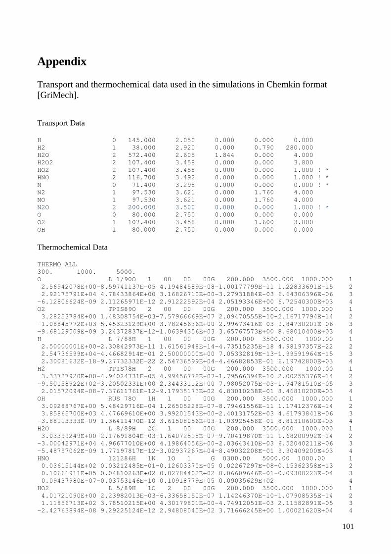
Appendix Transport and thermochemical data used in the simulations in Chemkin format [GriMech]. Transport Data H 0 145.000 2.050 0.000 0.000 0.000 H2 1 38.000 2.920 0.000 0.790 280.000 H2O 2 572.400 2.605 1.844 0.000 4.000 H2O2 2 107.400 3.458 0.000 0.000 3.800 HO2 2 107.400 3.458 0.000 0.000 1.000 ! * HNO 2 116.700 3.492 0.000 0.000 1.000 ! * N 0 71.400 3.298 0.000 0.000 0.000 ! * N2 1 97.530 3.621 0.000 1.760 4.000 NO 1 97.530 3.621 0.000 1.760 4.000 N2O 2 200.000 3.500 0.000 0.000 1.000 ! * O 0 80.000 2.750 0.000 0.000 0.000 O2 1 107.400 3.458 0.000 1.600 3.800 OH 1 80.000 2.750 0.000 0.000 0.000 Thermochemical Data THERMO ALL 300. 1000. 5000. O L 1/90O 1 00 00 00G 200.000 3500.000 1000.000 1 2.56942078E+00-8.59741137E-05 4.19484589E-08-1.00177799E-11 1.22833691E-15 2 2.92175791E+04 4.78433864E+00 3.16826710E+00-3.27931884E-03 6.64306396E-06 3 -6.12806624E-09 2.11265971E-12 2.91222592E+04 2.05193346E+00 6.72540300E+03 4 O2 TPIS89O 2 00 00 00G 200.000 3500.000 1000.000 1 3.28253784E+00 1.48308754E-03-7.57966669E-07 2.09470555E-10-2.16717794E-14 2 -1.08845772E+03 5.45323129E+00 3.78245636E+00-2.99673416E-03 9.84730201E-06 3 -9.68129509E-09 3.24372837E-12-1.06394356E+03 3.65767573E+00 8.68010400E+03 4 H L 7/88H 1 00 00 00G 200.000 3500.000 1000.00 1 2.50000001E+00-2.30842973E-11 1.61561948E-14-4.73515235E-18 4.98197357E-22 2 2.54736599E+04-4.46682914E-01 2.50000000E+00 7.05332819E-13-1.99591964E-15 3 2.30081632E-18-9.27732332E-22 2.54736599E+04-4.46682853E-01 6.19742800E+03 4 H2 TPIS78H 2 00 00 00G 200.000 3500.000 1000.00 1 3.33727920E+00-4.94024731E-05 4.99456778E-07-1.79566394E-10 2.00255376E-14 2 -9.50158922E+02-3.20502331E+00 2.34433112E+00 7.98052075E-03-1.94781510E-05 3 2.01572094E-08-7.37611761E-12-9.17935173E+02 6.83010238E-01 8.46810200E+03 4 OH RUS 78O 1H 1 00 00G 200.000 3500.000 1000.000 1 3.09288767E+00 5.48429716E-04 1.26505228E-07-8.79461556E-11 1.17412376E-14 2 3.85865700E+03 4.47669610E+00 3.99201543E+00-2.40131752E-03 4.61793841E-06 3 -3.88113333E-09 1.36411470E-12 3.61508056E+03-1.03925458E-01 8.81310600E+03 4 H2O L 8/89H 2O 1 00 00G 200.000 3500.000 1000.000 1 3.03399249E+00 2.17691804E-03-1.64072518E-07-9.70419870E-11 1.68200992E-14 2 -3.00042971E+04 4.96677010E+00 4.19864056E+00-2.03643410E-03 6.52040211E-06 3 -5.48797062E-09 1.77197817E-12-3.02937267E+04-8.49032208E-01 9.90409200E+03 4 HNO 121286H 1N 1O 1 G 0300.00 5000.00 1000.00 1 0.03615144E+02 0.03212485E-01-0.12603370E-05 0.02267297E-08-0.15362358E-13 2 0.10661911E+05 0.04810263E+02 0.02784402E+02 0.06609646E-01-0.09300223E-04 3 0.09437980E-07-0.03753146E-10 0.10918779E+05 0.09035629E+02 4 HO2 L 5/89H 1O 2 00 00G 200.000 3500.000 1000.000 1 4.01721090E+00 2.23982013E-03-6.33658150E-07 1.14246370E-10-1.07908535E-14 2 1.11856713E+02 3.78510215E+00 4.30179801E+00-4.74912051E-03 2.11582891E-05 3 -2.42763894E-08 9.29225124E-12 2.94808040E+02 3.71666245E+00 1.00021620E+04 4

101

H2O2 L 7/88H 2O 2 00 00G 200.000 3500.000 1000.000 1 4.16500285E+00 4.90831694E-03-1.90139225E-06 3.71185986E-10-2.87908305E-14 2 -1.78617877E+04 2.91615662E+00 4.27611269E+00-5.42822417E-04 1.67335701E-05 3 -2.15770813E-08 8.62454363E-12-1.77025821E+04 3.43505074E+00 1.11588350E+04 4 N 120186N 1 G 0300.00 5000.00 1000.00 1 0.02450268E+02 0.10661458E-03-0.07465337E-06 0.01879652E-09-0.10259839E-14 2 0.05611604E+06 0.04448758E+02 0.02503071E+02-0.02180018E-03 0.05420529E-06 3 -0.05647560E-09 0.02099904E-12 0.05609890E+06 0.04167566E+02 4 N2 121286N 2 G 0300.00 5000.00 1000.00 1 0.02926640E+02 0.14879768E-02-0.05684760E-05 0.10097038E-09-0.06753351E-13 2 -0.09227977E+04 0.05980528E+02 0.03298677E+02 0.14082404E-02-0.03963222E-04 3 0.05641515E-07-0.02444854E-10-0.10208999E+04 0.03950372E+02 4 NO 121286N 1O 1 G 0300.00 5000.00 1000.00 1 0.03245435E+02 0.12691383E-02-0.05015890E-05 0.09169283E-09-0.06275419E-13 2 0.09800840E+05 0.06417293E+02 0.03376541E+02 0.12530634E-02-0.03302750E-04 3 0.05217810E-07-0.02446262E-10 0.09817961E+05 0.05829590E+02 4 N2O 121286N 2O 1 G 0300.00 5000.00 1000.00 1 0.04718977E+02 0.02873713E-01-0.11974958E-05 0.02250551E-08-0.15753370E-13 2 0.08165811E+05-0.16572504E+01 0.02543057E+02 0.09492193E-01-0.09792775E-04 3 0.06263844E-07-0.01901825E-10 0.08765100E+05 0.09511222E+02 4 END Test Matrix

Test Case

Power [kW]

Disk Distance

[mm] Y %H2O in

air Φprim Φoverall 21 kW TVC-1 21 60 0 1.000 0.053 TVC-2 21 65 0 1.000 0.053 TVC-3 21 70 0 1.000 0.053 TVC-4 21 75 0 1.000 0.053 TVC-5 21 80 0 1.000 0.053 TVC-6 21 60 0.00338 1.000 0.053 TVC-7 21 65 0.00338 1.000 0.053 TVC-8 21 70 0.00338 1.000 0.053 TVC-9 21 75 0.00338 1.000 0.053 TVC-10 21 80 0.00338 1.000 0.053 TVC-11 21 60 0 1.000 0.029 TVC-12 21 65 0 1.000 0.029 TVC-13 21 70 0 1.000 0.029 TVC-14 21 75 0 1.000 0.029 TVC-15 21 80 0 1.000 0.029 42 kW TVC-16 42 60 0 1.465 0.103 TVC-17 42 65 0 1.465 0.103 TVC-18 42 70 0 1.465 0.103 TVC-19 42 75 0 1.465 0.103 TVC-20 42 80 0 1.465 0.103 TVC-21 42 60 0.00338 1.465 0.103 TVC-22 42 65 0.00338 1.465 0.103 TVC-23 42 70 0.00338 1.465 0.103 TVC-24 42 75 0.00338 1.465 0.103 TVC-25 42 80 0.00338 1.465 0.103 TVC-26 42 60 0 0.991 0.057 TVC-27 42 65 0 0.991 0.057 TVC-28 42 70 0 0.991 0.057

102

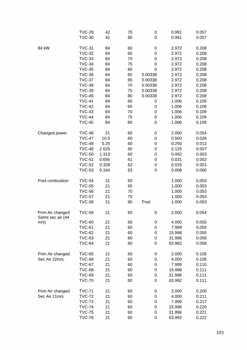
TVC-29 42 75 0 0.991 0.057 TVC-30 42 80 0 0.991 0.057 84 kW TVC-31 84 60 0 2.972 0.208 TVC-32 84 65 0 2.972 0.208 TVC-33 84 70 0 2.972 0.208 TVC-34 84 75 0 2.972 0.208 TVC-35 84 80 0 2.972 0.208 TVC-36 84 60 0.00338 2.972 0.208 TVC-37 84 65 0.00338 2.972 0.208 TVC-38 84 70 0.00338 2.972 0.208 TVC-39 84 75 0.00338 2.972 0.208 TVC-40 84 80 0.00338 2.972 0.208 TVC-41 84 60 0 1.006 0.109 TVC-42 84 65 0 1.006 0.109 TVC-43 84 70 0 1.006 0.109 TVC-44 84 75 0 1.006 0.109 TVC-45 84 80 0 1.006 0.109 Changed power TVC-46 21 60 0 2.000 0.054 TVC-47 10.5 60 0 0.500 0.026 TVC-48 5.25 60 0 0.250 0.013 TVC-49 2.625 60 0 0.125 0.007 TVC-50 1.313 60 0 0.062 0.003 TVC-51 0.656 61 0 0.031 0.002 TVC-52 0.328 62 0 0.016 0.001 TVC-53 0.164 63 0 0.008 0.000 Post combustion TVC-54 21 60 1.000 0.053 TVC-55 21 65 1.000 0.053 TVC-56 21 70 1.000 0.053 TVC-57 21 75 1.000 0.053 TVC-58 21 80 Post 1.000 0.053 Prim Air changed TVC-59 21 60 0 2.000 0.054Same sec air (44 m/s) TVC-60 21 60 0 4.000 0.055 TVC-61 21 60 0 7.999 0.055 TVC-62 21 60 0 15.998 0.055 TVC-63 21 60 0 31.996 0.056 TVC-64 21 60 0 63.992 0.056 Prim Air changed TVC-65 21 60 0 2.000 0.105Sec Air 22m/s TVC-66 21 60 0 4.000 0.108 TVC-67 21 60 0 7.999 0.110 TVC-68 21 60 0 15.998 0.111 TVC-69 21 60 0 31.996 0.111 TVC-70 21 60 0 63.992 0.111 Prim Air changed TVC-71 21 60 0 2.000 0.200Sec Air 11m/s TVC-72 21 60 0 4.000 0.211 TVC-73 21 60 0 7.999 0.217 TVC-74 21 60 0 15.998 0.220 TVC-75 21 60 0 31.996 0.221 TVC-76 21 60 0 63.992 0.222

103

104

Without Prim Air TVC-77 21 60 0.00338 0.056 TVC-78 21 65 0.00338 0.056 TVC-79 21 70 0.00338 0.056 TVC-80 21 75 0.00338 0.056 TVC-81 21 80 0.00338 0.056