NTS GCD 06 Supply and Demand Balancing Rules v2

DISCUSSION DOCUMENT

Modification Proposal to the Gas Transmission Transportation Charging Methodology

NTS GCD 06: Supply and Demand Balancing Rules in the Transportation Model

23rd February 2009

Table of Contents

EXECUTIVE SUMMARY ....................................................................................................................1

1 INTRODUCTION .........................................................................................................................2

2 BACKGROUND ..........................................................................................................................2

Current Methodology.................................................................................................................2

Short Term vs. Long Term Supply Forecasts ...........................................................................3

Minimum Price ..........................................................................................................................3

Reasons for moving away from the prevailing methodology ....................................................3

Considerations for a new methodology.....................................................................................3

3 DISCUSSION OF SUPPLY AND DEMAND BALANCING OPTIONS .......................................4

Proposed Options .....................................................................................................................6

National Grid’s View..................................................................................................................6

Key Price Driver ........................................................................................................................6

4 DISCUSSION OF SOURCE OF SUPPLY DATA .......................................................................7

Alternative Options....................................................................................................................7

National Grid’s View..................................................................................................................7

5 RELEVANT OBJECTIVES .........................................................................................................8

Assessment against Licence Objectives...................................................................................8

Assessment against EU Gas Regulations ................................................................................8

6 QUESTIONS FOR DISCUSSION ...............................................................................................9

APPENDIX A – ANALYSIS PRESENTED AT JANUARY 2009 TCMF...........................................10

APPENDIX B – FURTHER ANALYSIS – CONSTANT REVENUE .................................................23

APPENDIX C – FURTHER ANALYSIS – 2015/16, 2016/17 AND 2017/18.....................................24

National Grid

NTS GCD 06 1

Executive Summary

This document sets out for discussion options for revising the Gas Transmission Transportation Charging Methodology (the “Charging Methodology”) with respect to the rules applied to achieve a supply and demand flow match in the Transportation Model, which is used to set NTS Exit Capacity Prices and NTS Entry Auction Reserve Prices.

This document is issued by National Grid in its role as Gas Transporter Licence holder in respect of the NTS (“National Grid”).

The Transportation Model is used to set all entry capacity auction reserve prices and exit capacity prices. Like all network analysis models it requires supply to equal demand.

The Charging Methodology states that a supply and demand match is achieved in the Transportation Model by reducing supplies in a merit order to match the forecast demand.

Analysis carried out to support consultation paper NTS GCM 05: NTS Exit Flat Capacity Prices, highlighted some exit price volatility in areas close to supply points affected by the balancing rules and the supply merit order.

Changes to the supply and demand data in the Transportation Model have the potential to change the direction of the flow of gas and this is likely to noticeably impact prices.

It was noted that changing the supply and demand balancing rules could reduce the impact of supply changes on exit price variation.

National Grid recognises that Exit Reform could significantly reduce exit price volatility as prices are proposed to be set using baseline demand; however, we recognise that investigating methods of dampening entry and exit price volatility in the transitional period, prior to the introduction of Exit Reform, could be beneficial.

Discussions at recent Gas TCMF meetings have highlighted two potential factors contributing to price variation;

1. the methodology applied to achieve a supply and demand match in the Transportation Model.

2. the source of the supply data used to achieve a supply and match in the Transportation Model i.e. the Ten Year Statement

This discussion paper takes forward the analysis presented at the July 2008, November 2008 and January 2009 Gas TCMF meetings.

The paper sets out four potential options for achieving a supply and demand flow match within the Transportation Model and seeks views on the source of supply data.

The closing date for submission of your responses to this consultation is 20th March 2009

National Grid

NTS GCD 06 2

1 Introduction

1.1 The Transportation Model is used to set all entry capacity auction reserve prices and exit capacity prices. Like all network analysis models it requires supply to equal demand.

1.2 Currently the inputs to the Transportation Model are:

� Forecast 1-in-20 peak day demand data

� Supply data from the Ten Year Statement

With the introduction of Exit Reform from gas year 2012/13 the demand data used in the Transportation Model is proposed to be baseline exit demand with bi-directional sites assumed to be in supply mode i.e. with zero exit flow.

1.3 The Charging Methodology states that a supply and demand match is achieved in the Transportation Model by reducing supplies in a merit order to match the forecast demand.

1.4 Analysis carried out to support consultation paper NTS GCM 05: NTS Exit Flat Capacity Prices, highlighted some exit price volatility in areas close to supply points affected by the balancing rules and the supply merit order.

1.5 Changes to the supply and demand data in the Transportation Model have the potential to change the direction of the flow of gas and this is likely to noticeably impact prices.

1.6 It was noted that changing the supply and demand balancing rules could reduce the impact of supply changes on exit price variation.

2 Background

Current Methodology

2.1 The supply data used in the Transportation Model is derived from the data set out in the most recent Ten Year Statement for each gas year for which prices are being set.

2.2 A supply and demand match is achieved at peak conditions by reducing supplies, as required, in a merit order to match the forecast demand. Supply points are “turned off” one by one until a match is achieved, starting with the supplies in group 1 from the list below and moving on to the supplies in group 2 when all group 1 supplies have been reduced to zero. Within each group individual entry points are assigned a value in the merit order. The order for reducing supplies is as follows;

1. Short-range storage facilities (LNG)

2. Mid-range storage facilities

3. Long-range storage facilities (Rough)

4. Interconnectors (BBL and IUK)

5. LNG importation facilities (Isle of Grain and Milford Haven)

6. Beach terminals including on-shore fields (Bacton, Barrow, Burton Point, Easington, St Fergus, Teesside, Theddlethorpe, Wytch farm).

In practice the supplies in groups 3 – 6 inclusive have always been fully utilised.

National Grid

NTS GCD 06 3

2.3 The merit order for the storage sites is determined by National Grid based on the injection and withdrawal rates of the storage facilities. The lower the ratio of injection to withdrawal, the higher up the merit order the facility will be. Supplies will be “turned off” starting from the top of the merit order.

2.4 With the introduction of Exit Reform and the proposed use of baseline exit capacity for charge setting, it is possible that the supplies in the Ten Year Statement will not be sufficient to meet demand. This may be due to forecast supplies being less than the relevant entry point capability. Alternate supply data sources are considered further in section 4.

Short Term vs. Long Term Supply Forecasts

2.5 Prior to the implementation of the Transportation Model in 2007, entry and exit capacity prices were set using the engineering model Transcost. The supply data that was entered into Transcost was ten years’ worth of forecasted supply data.

2.6 Consultation Paper NTS GCM 01 proposed that with the implementation of the Transportation Model a single year’s forecasted supply and demand data should be used, rather than a ten year forecast. This avoids potential distortions created by inaccurate long term forecasts and avoids the circularity caused by use of supply forecasts to generate prices for long term capacity auctions, which are designed to signal such supply requirements.

Minimum Price

2.7 The minimum entry and exit capacity price in the Transportation Model is 0.0001p/kWh as negative capacity prices would give a perverse incentive to Users to book more capacity than would otherwise be required, potentially leading to inefficient development and operation of the NTS.

Planning Process

2.8 While National Grid continues to produce a single central case supply forecast within the Ten Year Statement, the planning approach has now moved away from using a strict merit order for generating supply and demand matches and so the merit order may no longer be the most appropriate method of balancing supply and demand in the Transportation Model.

Reasons for moving away from the prevailing methodology

2.9 Matching demand by turning on supply points one by one (merit order) can produce variable prices which may not appropriately reflect underlying costs.

2.10 When LNG storage is intermittently required to match the demand level it is likely to impact on entry and exit prices in the surrounding area.

2.11 Exit prices will vary as a consequence of demand changes (which is appropriate) but changing the supply and demand balancing rules could minimise the impact of supply changes on exit price variation.

Considerations for a new methodology

2.12 The methodology should reflect the costs that have been incurred in developing the NTS to facilitate entry and exit capacity.

2.13 A more transparent approach could be of benefit.

National Grid

NTS GCD 06 4

Cost Reflectivity vs. Price Stability

2.14 Prior to the implementation of the Transportation Model, exit capacity price capping rules were employed to forge a level of stability and predictability of prices from year to year; however, these rules eroded genuine cost reflectivity and were therefore removed with the introduction of the Transportation Model. Over time, excessive emphasis on stability could result in a significant departure from cost reflectivity.

2.15 It is National Grid’s view that competition can be promoted in terms of the development of the Charging Methodology by making it simple and easy to understand such that prices can be replicated and forecast by Users. More stable prices may lead to ease in forecasting.

2.16 Charge stability or predictability might be justified with reference to User cost-base planning ability. Users should not experience volatile charges year on year.

2.17 In accordance with the NTS Licence relevant charging objectives (as outlined in section 5 of this document), cost-reflectivity is the dominating objective.

3 Discussion of Supply and Demand Balancing Options

3.1 Through the Gas TCMF, alternative supply and demand options were identified and discussed. At the November 2008 TCMF National Grid compared the current merit order approach, used to match supply and demand flows in the Transportation Model, and six alternative approaches outlined below:

3.2 Option One: Prevailing Methodology

A supply and demand match is achieved at peak conditions by reducing supplies, as required, in a merit order to match the forecast demand. Supply points are “turned off” one by one until a match is achieved, starting with the supplies in group 1 from the list below and moving on to the supplies in group 2 when all group 1 supplies have been reduced to zero. Within each group, individual entry points are assigned a value in the merit order. The order for reducing supplies is as follows;

1. Short-range storage facilities (LNG)

2. Mid-range storage facilities

3. Long-range storage facilities (Rough)

4. Interconnectors (BBL and IUK)

5. LNG importation facilities (Isle of Grain and Milford Haven)

6. Beach terminals including On-shore Fields (Bacton, Barrow, Burton Point, Easington, St Fergus, Teesside, Theddlethorpe, Wytch Farm).

In practice the supplies in groups 3 – 6 inclusive are always fully utilised.

3.3 Option Two

All supplies, as listed under Option One, are scaled by an equal percentage to meet demand. The percentage will be calculated as the total demand included within the model divided by total available supplies.

National Grid

NTS GCD 06 5

3.4 Options Three to Seven

Under these options each supply group is fully utilised in turn and the supplies in the last required group are scaled by an equal percentage to achieve a supply and demand match. An example follows Option Three to explain this further.

3.5 Option Three

Supplies are split into three groups:

1) Beach, Interconnectors, LNG Importation, Long-range Storage (Rough) 2) Mid-range Storage 3) Short-range Storage (LNG)

Example

Demand is 6350GWh, available supply is 6709GWh and we need to achieve a supply and demand balance using option three. The breakdown of available supply as given by the Ten Year Statement is:

Group 1: Beach, Interconnectors, LNG Importation, Long-range Storage – 5503GWh

Group 2: Mid-range Storage – 682GWh

Group 3: Short-range Storage – 524GWh

To meet demand we need to fully utilise the supplies in Group 1 and Group 2 and use a percentage of the supplies in Group 3:

Group 1 + Group 2 = 5503GWh + 682GWh = 6185GWh

Shortfall = 6350GWh-6185GWh = 165GWh

Percentage required from each supply point in Group 3 = 165GWh / 524GWh = 31%

3.6 Option Four

Supplies are split into three groups:

1) Beach, Interconnectors, Long-range Storage (Rough), Mid-range Storage

2) LNG Importation 3) Short-range Storage (LNG)

3.7 Option Five

Supplies are split into two groups:

1) Beach, Interconnectors, Long-range Storage (Rough) 2) Mid-range Storage, LNG Importation, Short-range Storage (LNG)

3.8 Option Six


1) Beach, Interconnectors, LNG Importation, Long-range Storage (Rough) 2) Mid-range Storage, Short-range Storage (LNG)

National Grid

NTS GCD 06 6

3.9 Option Seven


1) Beach, Interconnectors, Long-range Storage (Rough), Mid-range Storage

2) LNG Importation, Short-range storage (LNG)

Proposed Options

3.10 At the November 2008 Gas TCMF, Options Two, Four, and Seven were either identified as operationally unrealistic or as producing volatile entry and exit capacity prices and were subsequently discarded. Option Two is equivalent to the charging methodology applied by National Grid Electricity Transmission in the calculation of the Transmission Network Use of System Tariff.

3.11 It is National Grid’s view that Option Two is unsuitable for use in the calculation of gas NTS entry and exit capacity prices because of the different scheduling and planning approaches used in gas and electricity.

3.12 Further analysis on rules One, Three, Five and Six was presented at the January 2009 TCMF. The presentation can be found in Appendix A.

National Grid’s View

3.13 It is National Grid’s view that Option One is no longer an appropriate method for balancing supply and demand flow levels in the Transportation Model as it does not appropriately reflect the planning and development of the NTS.

3.14 Options Three, Five and Six are all transparent and would allow the Industry to replicate National Grid’s charge setting process more accurately, particularly with the introduction of new entry points.

3.15 National Grid’s preferred option is Option Three where supplies are split into three groups as follows:

1) Beach, Interconnectors, LNG Importation, Long-range Storage (Rough)

2) Mid-range Storage 3) Short-range Storage (LNG)

These groups represent well defined behaviours across the different types of supply more accurately than Options Five and Six and are non-discriminatory

between the different baseload-type supplies.

Key Price Driver

3.16 Entry and exit capacity prices are governed by how far gas has to travel through the NTS; the further it travels the higher the price will be.

3.17 Using supply data that steadily increases / decreases at storage ASEPs each year (i.e. using an equal percentage of supply from each ASEP) to match an increase / decrease in demand should produce more stable prices.

3.18 Changes to the supply and demand data in the Transportation Model have the potential to change the direction of the flow of gas and this is likely to noticeably impact prices.

National Grid

NTS GCD 06 7

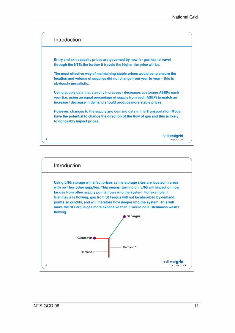
3.19 Using LNG storage will affect prices as the storage sites are located in areas with no or few other supplies. This means “turning on” LNG will impact on how far gas from other supply points flows into the system. For example, if Glenmavis is flowing, gas from St Fergus will not be absorbed by demand points so quickly, and will therefore flow deeper into the system. This will make the St Fergus entry capacity prices more expensive than it would be if Glenmavis wasn’t flowing.

4 Discussion of Source of Supply Data

4.1 Discussions with the Industry at recent Gas TCMF meetings have focussed on the source of the supply data used to match demand in the Transportation Model. It was suggested that fluctuations in the Ten Year Statement from year to year play a large role in the volatility of entry and exit capacity prices and that National Grid should explore different sources of supply data.

Alternative Options

4.2 Historical Data

It was suggested that using historical flow data could provide more stable supply levels from year to year than those forecasted in the Ten Year Statement, however, historical data would be unavailable for new sites and it could be inappropriate to apply to future years for sites where supplies are declining. This could make the data inconsistent and inaccurate.

4.3 Obligated1 Entry Capacity

Using obligated entry capacity levels as the source of supply data used to match demand has potential but there is often a significant difference between obligated entry capacity, and actual bookings and anticipated flow levels.

4.4 Physical Capability

Using physical capability to determine available supplies to match demand is an alternative option. While this would be relatively straightforward in terms of storage, LNG importation and interconnectors it would prove difficult for beach terminals. The likely flow capability for beach terminals would be limited by the connected off-shore fields.

4.5 Combinations of Supply Data

It may be possible to overcome some of the issues of obligated entry capacity and physical capability by using a combination of data. One option could be to use Ten Year Statement supply data for beach terminals and either obligated entry capacity or physical capability for other entry points.

National Grid’s View

4.6 It is National Grid’s view that, at this time, the Ten Year Statement remains the most appropriate source of beach supply data to be used to match demand flow levels in the Transportation Model, however, further consideration should be given to storage, interconnectors and LNG importation.

1 Obligated Entry Capacity = Baseline Entry Capacity + Incremental Entry Capacity +/- Substituted Entry

Capacity

National Grid

NTS GCD 06 8

4.7 National Grid recognises that fluctuations in the Ten Year Statement from year to year can create volatile capacity prices. A potential approach to dampening this volatility would be to average supply data from a number of Ten Year Statements to smooth the fluctuations whilst maintaining a level of operational reality and cost reflectivity.

5 Relevant Objectives

Assessment against Licence Objectives

5.1 The National Grid plc Gas Transporter Licence in respect of the NTS requires that proposed changes to the NTS Charging Methodology shall achieve the relevant methodology objectives. Respondents are therefore asked to consider how the different options would best satisfy the relevant objectives as part of their responses to this discussion paper.

5.2 Where transportation prices are not established through an auction, prices calculated in accordance with the methodology should:

� 1) Reflect the costs incurred by the licensee in its transportation business;

� 2) So far as is consistent with (1) properly take account of developments in the transportation business;

� 3) So far as is consistent with (1) and (2) facilitate effective competition between gas shippers and between gas suppliers.

Assessment against EU Gas Regulations

5.3 EC Regulation 1775/2005 on conditions for access to the natural gas transmission networks (binding from 1 July 2006) are summarised below.

� The principles for network access tariffs or the methodologies used to calculate them shall:

o Be transparent

o Take into account the need for system integrity and its improvement

o Reflect actual costs incurred for an efficient and structurally comparable network operator

o Be applied in a non-discriminatory manner

o Facilitate efficient gas trade and competition

o Avoid cross-subsidies between network users

o Provide incentives for investment and maintaining or creating interoperability for transmission networks

o Not restrict market liquidity

o Not distort trade across borders of different transmission systems.

National Grid

NTS GCD 06 9

6 Questions for Discussion

National Grid would welcome responses on the following areas discussed in the paper to inform the development of a charging methodology:

Supply & Demand Balancing Rules

� Q1. Do respondents consider the preferred option, Rule Three, to be transparent and cost reflective?

� Q2. Do respondents consider any of the alternative options to be more transparent and cost reflective?

� Q3. Do respondents consider an option differing from those proposed to be more transparent and cost reflective?

Supply Availability

� Q4: Do respondents consider averaging supply data from a number of Ten Year Statements to be an appropriate approach to dampening entry and exit price volatility?

� Q5: For each of the four supply types; Beach, Interconnector, LNG Importation and Storage, which data source do respondents consider to be most appropriate to use for charge setting purposes?

� Obligated Entry Capacity

� Physical Capability

� Ten Year Statement

� Q6: Do respondents consider alternative sources of supply data to be more appropriate?

General

� Q7: What further analysis would respondents like to be included with any future consultation?

The closing date for submission of your responses is 20th March 2009. Your response should be e-mailed to:

[email protected]

or alternatively sent by post to:

Jemma Spencer, Regulatory Frameworks, National Grid, National Grid House, Gallows Hill, Warwick, CV34 6DA.

If you wish to discuss any matter relating to this charge methodology consultation then please call Eddie Blackburn � 01926 656022, Debra Hawkin � 01926 656317 or Jemma Spencer � 01926 654212

Responses to this discussion paper may be incorporated within National Grid’s subsequent consultation paper. If you wish your response to be treated as confidential then please mark it clearly to that effect.

National Grid

NTS GCD 06 10

Appendix A – Analysis Presented at January 2009 TCMF

Capacity Prices and Supply & Demand Balancing Options

Gas TCMF

8th January 2009

2

Introduction

At the 6th November 2008 Gas TCMF we presented analysis that compared

the NTS entry and exit capacity prices generated under the current merit order

approach for balancing supply & demand within the Transportation Model and

six potential alternative approaches.

Issues discussed included whether we are seeking to find the approach that

produces the least volatile entry and exit prices or that which most closely

reflects operational reality.

Three options were discarded.

National Grid

NTS GCD 06 11

3

Introduction

Entry and exit capacity prices are governed by how far gas has to travel

through the NTS; the further it travels the higher the price will be.

The most effective way of maintaining stable prices would be to ensure the

location and volume of supplies did not change from year to year – this is

obviously unrealistic.

Using supply data that steadily increases / decreases at storage ASEPs each

year (i.e. using an equal percentage of supply from each ASEP) to match an

increase / decrease in demand should produce more stable prices.

However, changes to the supply and demand data in the Transportation Model

have the potential to change the direction of the flow of gas and this is likely

to noticeably impact prices.

4

Introduction

Using LNG storage will affect prices as the storage sites are located in areas

with no / few other supplies. This means ‘turning on’ LNG will impact on how

far gas from other supply points flows into the system. For example, if

Glenmavis is flowing, gas from St Fergus will not be absorbed by demand

points so quickly, and will therefore flow deeper into the system. This will

make the St Fergus gas more expensive than it would be if Glenmavis wasn’t

flowing.St Fergus

Glenmavis

Demand 1

Demand 2

National Grid

NTS GCD 06 12

5

Supply and Demand Scenarios

� GCM05 Demand Scenarios - 2012/13 Transportation Model

� Demand scenarios

� As-is (Firm only)

� Demand Scenario 1 (forecast firm demand plus DC interruptible)

� Demand Scenario 2 (forecast firm demand plus DC & DN interruptible)

N.B. Demand Scenario 3 from GCM05 not used in this analysis as it used the same supply and demand

information as scenario 2 but with a higher IUK booked capacity

� Supply data taken from 2007 Ten Year Statement

� Current merit order approach and six alternative approaches considered

November ‘08 Analysis

6

Supply and Demand Balancing Rules - Options

Rule 1: Supplies ranked by Merit Order as per prevailing methodology

Under Rules 3, 5 & 6, each supply group is fully utilised in order. Each of the supplies in the

last required group is scaled down by an equal percentage.

Rule 3: Supplies split into three groups:

1. Beach, Interconnectors, LNG Importation, Long-Range Storage (Rough)

2. Mid-Range Storage

3. Short-Range Storage (LNG)

Rule 5: Supplies split into two groups and utilised as follows:

1. Beach, Interconnectors, Long-Range Storage

2. LNG Importation, Mid-Range Storage, Short-Range Storage (LNG)

Rule 6: Supplies split into two groups and utilised as follows:


2. Mid-Range Storage, Short-Range Storage (LNG)

National Grid

NTS GCD 06 13

7

Analysis

� Calculated entry and exit prices for the three demand scenarios under each rule

� Calculated the range of prices across the three demand scenarios for all entry and

exit points under each rule

� The following entry & exit graphs show, across the three demand scenarios under

each rule:

� The average price range across the three demand levels for all entry and exit points

� The maximum price range for an entry/exit point

� The standard deviation of price ranges


8

Example

0.0018

0.0000

0.0040

Price Range

0.0073

0.0001

0.0006

Scenario 2

0.00010.0001Exit Point 2

0.00550.0061Exit Point 3

0.00180.0046Exit Point 1

Scenario 1As-Is

The below table contains the exit prices (p/kWh/day) for three example exit points analysed under Rule 1:

The average price range is 0.0019 p/kWh/day

The maximum price range is 0.0040 p/kWh/day

The standard deviation of the price range is 0.0020 p/kWh/day


National Grid

NTS GCD 06 14

9

Impact of S&D Balancing Options on Entry Price Variation

0.0000

0.0005

0.0010

0.0015

0.0020

0.0025

0.0030

0.0035

0.0040

Rule 1 Rule 3 Rule 5 Rule 6

p/k

Wh

/da

y

Average of the Entry Reserve Price RangeMaximum Entry Reserve Price RangeStandard Deviation for the Entry Reserve Price Range

November ‘08

Analysis

10

Impact of S&D Balancing Options on Exit Price Variation

0.0000

0.0010

0.0020

0.0030

0.0040

0.0050

0.0060

0.0070

0.0080


p/k

Wh

/da

y

Average of the Offtake Exit Price RangeMaximum Offtake Exit Price RangeStandard Deviation for the Offtake Exit Price Range

November ‘08

Analysis

National Grid

NTS GCD 06 15

11

Results

� Rule 3 produces the least variable entry and exit prices across the three

scenarios.

� Rule 3: Supplies split into the following three groups:


2. Mid-Range Storage

3. Short-Range Storage (LNG)

However, the supply/demand scenarios used in this analysis have not required the use of LNG

Storage under Rule 3.

� Rule 6 could produce more stable prices in scenarios with more demand variation.

� Rule 6: Supplies split into the following two groups:


2. Mid-Range Storage, Short-Range Storage (LNG)

November ‘08

Analysis

12

Further Analysis

� Following the concerns raised by Ofgem regarding GCM05 and the direction for

implementation of UNC 0195AV (to be confirmed) further analysis has been carried

out

� The revised GCM05 proposal, where exit prices would be adjusted to collect TO

allowed revenue from the baseline (rather than the booked) level of capacity with

the costs associated with unsold baseline being commoditised should lead to more

stable exit prices as the level of baseline capacity should be more stable (and

predictable) than the level of booked capacity.

National Grid

NTS GCD 06 16

13

Supply and Demand Scenarios

� Three years modelled – 2012/13, 2013/14, 2014/15

� Baseline Exit Demand from Licence

� Supply from December 2008 Ten Year Statement for 2012/13, 2013/14 and 2014/15

January ‘09

Analysis

14

Entry Capacity Price Variation across years 2012/13,

2013/14 and 2014/15 (using 2008 TYS)

0.0000

0.0005

0.0010

0.0015

0.0020

0.0025

0.0030

0.0035

0.0040

0.0045

0.0050


p/k

Wh

/da

y


January ‘09 Analysis

National Grid

NTS GCD 06 17

15

Exit Capacity Price Variation across years 2012/13,

2013/14 and 2014/15 (using 2008 TYS)

0.0000

0.0010

0.0020

0.0030

0.0040

0.0050

0.0060

0.0070

0.0080


p/k

Wh

/da

y


January ‘09

Analysis

16

Summary

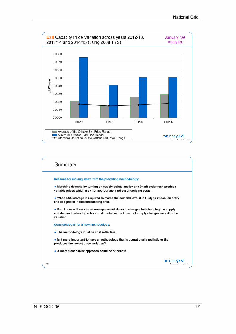
Reasons for moving away from the prevailing methodology:

� Matching demand by turning on supply points one by one (merit order) can produce

variable prices which may not appropriately reflect underlying costs.

� When LNG storage is required to match the demand level it is likely to impact on entry

and exit prices in the surrounding area.

� Exit Prices will vary as a consequence of demand changes but changing the supply

and demand balancing rules could minimise the impact of supply changes on exit price

variation

Considerations for a new methodology:

� The methodology must be cost reflective.

� Is it more important to have a methodology that is operationally realistic or that

produces the lowest price variation?

� A more transparent approach could be of benefit.

National Grid

NTS GCD 06 18

17

Next Steps

� Discussion Paper or Consultation Paper?

� Potential timeline

� Discussion Paper February 2009

� Discussion Report?

� Consultation and Indicative prices (150 days notice) 1st May 2009

� Final Proposals 1st July 2009

� Prices published 1st August 2009

� Implement 1st October 2009

18

Appendix

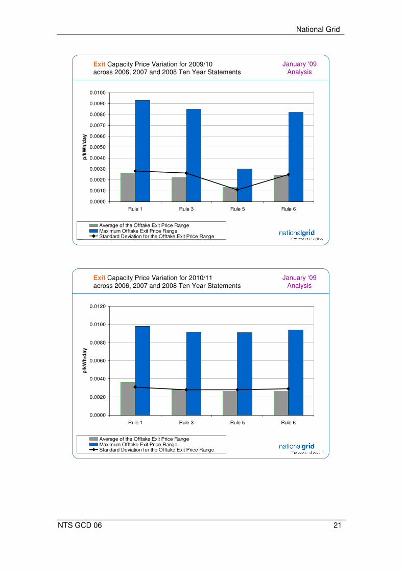
The following graphs show the results from comparisons of Rules 1, 3, 5 and 6 when considering the 2008/09, 2009/10 and 2010/11 Transportation Models using supply data from the last three published Ten Year Statements (in 2006, 2007 and 2008)

The first six graphs compare entry and exit prices under each rule when using supply data from each of the three Ten Year Statements i.e. comparing indicative and actual prices.

The last two graphs compare entry and exit prices under each rule comparing prices in 2008/09, 2009/10 and 2010/11


National Grid

NTS GCD 06 19

19

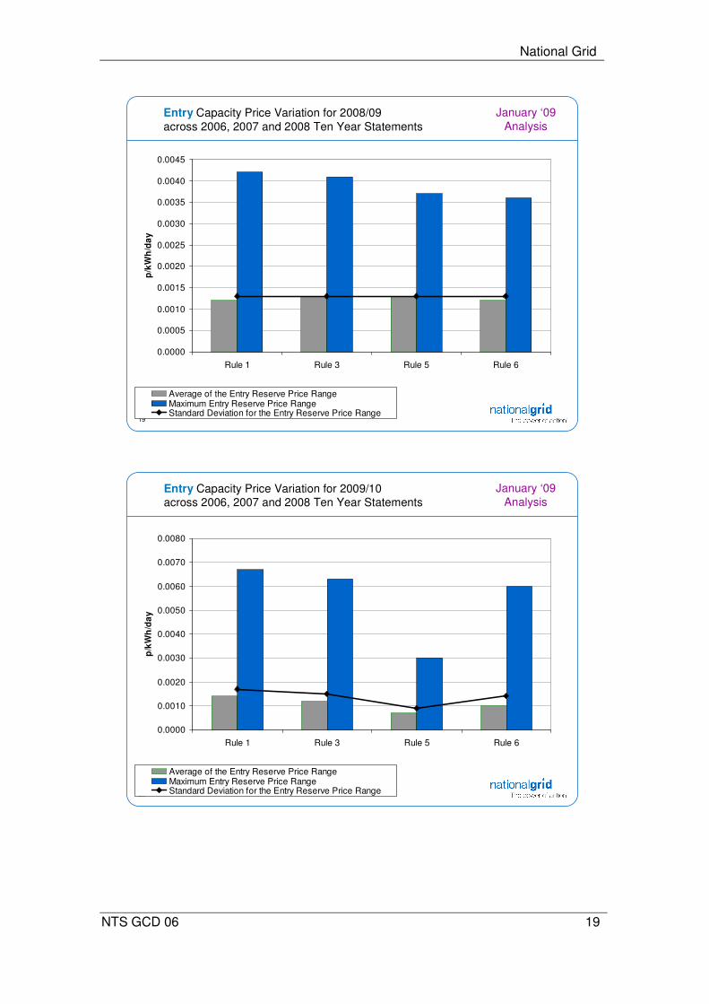
Entry Capacity Price Variation for 2008/09

across 2006, 2007 and 2008 Ten Year Statements

0.0000

0.0005

0.0010

0.0015

0.0020

0.0025

0.0030

0.0035

0.0040

0.0045


p/k

Wh

/da

y


January ‘09

Analysis

20

Entry Capacity Price Variation for 2009/10 across 2006, 2007 and 2008 Ten Year Statements

0.0000

0.0010

0.0020

0.0030

0.0040

0.0050

0.0060

0.0070

0.0080


p/k

Wh

/da

y


January ‘09

Analysis

National Grid

NTS GCD 06 20

21

Entry Capacity Price Variation for 2010/11 across 2006, 2007 and 2008 Ten Year Statements

0.0000

0.0010

0.0020

0.0030

0.0040

0.0050

0.0060

0.0070

0.0080


p/k

Wh

/da

y



22

Exit Capacity Price Variation for 2008/09 across 2006, 2007 and 2008 Ten Year Statements

0.0000

0.0020

0.0040

0.0060

0.0080

0.0100

0.0120

0.0140

0.0160


p/k

Wh

/da

y



National Grid

NTS GCD 06 21

23

Exit Capacity Price Variation for 2009/10 across 2006, 2007 and 2008 Ten Year Statements

0.0000

0.0010

0.0020

0.0030

0.0040

0.0050

0.0060

0.0070

0.0080

0.0090

0.0100


p/k

Wh

/da

y


January ‘09

Analysis

24

Exit Capacity Price Variation for 2010/11

across 2006, 2007 and 2008 Ten Year Statements

0.0000

0.0020

0.0040

0.0060

0.0080

0.0100

0.0120


p/k

Wh

/da

y


January ‘09

Analysis

National Grid

NTS GCD 06 22

25

Entry Capacity Price Variation across years 2008/09 (using 2007 TYS), 2009/10 (2008 TYS) and 2010/11 (2008 TYS) Transportation Models

0.0000

0.0010

0.0020

0.0030

0.0040

0.0050

0.0060


p/k

Wh

/da

y



26

Exit Capacity Price Variation across years 2008/09 (using 2007 TYS),

2009/10 (2008 TYS) and 2010/11 (2008 TYS) Transportation Models

0.0000

0.0010

0.0020

0.0030

0.0040

0.0050

0.0060

0.0070

0.0080


p/k

Wh

/da

y


January ‘09

Analysis

National Grid

NTS GCD 06 23

Appendix B – Further Analysis – Constant Revenue

At the January 2009 TCMF the attendees requested that National Grid show the entry and exit price variation across 2012/13, 2013/14, 2014/15 using the same revenue for the three years. The results of this analysis are presented below.

2

0.0000

0.0010

0.0020

0.0030

0.0040

0.0050

0.0060

0.0070

0.0080


p/k

Wh

/da

y


Entry Capacity Price Variation across years 2012/13, 2013/14 and

2014/15 (using 2008 TYS and constant revenue)

3

Exit Capacity Price Variation across years 2012/13, 2013/14

and 2014/15 (using 2008 TYS and constant revenue)

0.0000

0.0010

0.0020

0.0030

0.0040

0.0050

0.0060

0.0070

0.0080


p/k

Wh

/da

y


National Grid

NTS GCD 06 24

Appendix C – Further Analysis – 2015/16, 2016/17 and 2017/18

At the January 2009 TCMF the attendees requested that National Grid extend the analysis to look at 2015/16, 2016/17 and 2017/18 to consider the results when new storage sites begin flowing. The results are presented below.

4

0.0000

0.0010

0.0020

0.0030

0.0040

0.0050

0.0060

0.0070

0.0080


p/k

Wh

/da

y


Entry Capacity Price Variation across years 2015/16, 2016/17 and 2017/18 (using 2008 TYS and constant revenue)

5

Exit Capacity Price Variation across years 2015/16, 2016/17

and 2017/18 (using 2008 TYS and constant revenue)

0.0000

0.0010

0.0020

0.0030

0.0040

0.0050

0.0060

0.0070

0.0080


p/k

Wh

/da

y


NTS GCD 06 Supply and Demand Balancing Rules v2

Documents

Transcript of NTS GCD 06 Supply and Demand Balancing Rules v2