Novel and Powerful 3D Adaptive Crisp Active Contour Method...

Novel and Powerful 3D Adaptive Crisp Active Contour

Method applied in the Segmentation of CT Lung Images

Pedro Pedrosa Reboucas Filhoa, Paulo Cesar Cortezb, Antonio C. da SilvaBarrosc, Victor Hugo C. Albuquerquec, Joao Manuel R. S. Tavaresd

aLaboratorio de Processamento de Imagens e Simulacao Computacional, InstitutoFederal de Educacao, Ciencia e Tecnologia do Ceara, Maracanau, CE, Brazil

bDepartamento de Engenharia de Teleinformatica, Universidade Federal do Ceara,Fortaleza, CE, Brazil

cPrograma de Pos-Graduacao em Informatica Aplicada, Laboratorio de Bioinformatica,Universidade de Fortaleza, Fortaleza, Ceara, Brazil

dInstituto de Ciencia e Inovacao em Engenharia Mecanica e Engenharia Industrial,Departamento de Engenharia Mecanica, Faculdade de Engenharia, Universidade do

Porto, Porto, Portugal

Abstract

TheWorld Health Organization estimates that 300 million people have asthma,210 million people have Chronic Obstructive Pulmonary Disease (COPD),and, according to WHO, COPD will become the third major cause of deathworldwide in 2030. Computational Vision systems are commonly used inpulmonology to address the task of image segmentation, which is essentialfor accurate medical diagnoses. Segmentation defines the regions of the lungsin CT images of the thorax that must be further analyzed by the system orby a specialist physician. This work proposes a novel and powerful techniquenamed 3D Adaptive Crisp Active Contour Method (3D ACACM) for thesegmentation of CT lung images. The method starts with a sphere withinthe lung to be segmented that is deformed by forces acting on it towards thelung borders. This process is performed iteratively in order to minimize anenergy function associated with the 3D deformable model used. In the exper-

∗Corresponding author’s email: [email protected] addresses: [email protected] (Pedro Pedrosa Reboucas Filho),

[email protected] (Paulo Cesar Cortez), [email protected](Antonio C. da Silva Barros), [email protected] (Victor Hugo C.Albuquerque), [email protected] (Joao Manuel R. S. Tavares)

Preprint submitted to Medical Image Analysis August 31, 2016

imental assessment, the 3D ACACM is compared against three approachescommonly used in this field: the automatic 3D Region Growing, the level-setalgorithm based on coherent propagation and the semi-automatic segmenta-tion by an expert using the 3D OsiriX toolbox. When applied to 40 CT scansof the chest the 3D ACACM had an average F-measure of 99.22%, revealingits superiority and competency to segment lungs in CT images.

Keywords: CT scan; Image Segmentation; 3D Reconstruction; LungStructures.

1. Introduction

Several diseases that affect the world population are related to the lungs,for example: asthma (Kwan et al., 2015; Wisniewski and Zielinski, 2015),bronchiectasis (Arunkumar, 2012) and chronic obstructive pulmonary disease(COPD) (Mieloszyk et al., 2014; Ramalho et al., 2014; Spina et al., 2015).

The World Health Organization (WHO) estimates that 300 million peoplehave asthma, and this disease causes about 250 thousand deaths per yearworldwide (Campos and Lemos, 2009). Also, 210 million people have COPDand more than 300 thousand people died in 2005 from this disease (WHO,2014). Recent studies have shown that COPD is present in the 20 to 45 year-old-age bracket, although people over 50 years old are the most commonlyaffected. Additionally, WHO estimates that COPD will be the third majorcause of death worldwide by 2030 (Marco et al., 2004). For example, inBrazil from 1992 to 2006, 15% of all hospital admissions financed by thenational public health system were due to respiratory diseases, and asthmaand COPD together were responsible for 562,016 cases (Campos and Lemos,2009).

Hence, early effective diagnosis of lung diseases is urgently needed inpublic health. Among the factors that contribute to achieve this goal is theincreased accuracy of the diagnoses made by specialized physicians with theaid of computational vision systems. Additionally, some computational tech-niques can monitor patients with asthma and COPD using personal devices.Examples that can be highlighted among these techniques are the works ofKwan et al. (2015) and Juen et al. (2015).

In pulmonology, computed tomography (CT) imaging is often used as atool for detection and monitoring of diseases. Hence, CT images have beenused in the analysis of airways (Pu et al., 2011; Lo et al., 2012), vessels

2

(Korfiatis et al., 2011), cancer nodules (Diciotti et al., 2011), pulmonarylobes (Van Rikxoort et al., 2010), pulmonary emphysema (Sorensen et al.,2012; Hame et al., 2014), and fibrosis (Ariani et al., 2014) among otherlung diseases. Additionally, computational vision systems have been usedas diagnostic tools, particularly to address image segmentation, which is anessential step to assure correct and accurate results, by identifying the regionof the lungs in the CT thorax images that must be further analyzed by thesystem or by specialists.

The segmentation of objects or structures in medical images is usuallymore complex than in other types of images. Furthermore, in the case oflung images, this difficulty is due to the variability of the structures andthe internal organs of the lungs that can be imaged from different planes.Also, diseases can affect these organs, increasing the difficulty even more todevelop effective techniques to segment the images under study (ReboucasFilho et al., 2011, 2013).

Various lung segmentation techniques have been developed in recent years.Among these techniques, the 3D Region Growing (3D RG) approach has beenapplied to segment the lung and related internal structures, such as the ves-sels and airways (Born et al., 2009; Irving et al., 2009; Tschirren et al., 2009;Matsuoka et al., 2010; De Nunzio et al., 2011). Commercial software packagescommonly combine the 3D RG approach and Human Anatomy information,like HU density ranges, to aid image-based medical diagnoses. However, acorrect analysis is more difficult when there is a disease in the lungs. Thework of Nemec et al. (2015) studied and evaluated four software packagescommonly used to extract the lung volume of healthy volunteers from CTimages of the chest.

Among the softwares available, OsiriX from the University of Geneva(http://osirix-viewer.com/ ) is widely used for viewing and rendering 3D med-ical images (Canas et al., 2007; Martin et al., 2013; Wink, 2014). This soft-ware has automatic and semi-automatic tools for 3D segmentation (MichaelP Chae, 2015; Presti et al., 2015). In semi-automatic segmentation, an ex-pert analyzes the 3D objects under analysis and removes unwanted objectsusing the 3D Toolbox (Michael P Chae, 2015).

Wang et al. (2011, 2014) developed a fast level-set algorithm based onthe coherent propagation method and assessed its use on clinical datasets.The results indicated that this algorithm was about 10 times faster than theITK Snap software in the segmentation of medical images.

Mansoor et al. (2014) presented a solution to segment healthy and dis-

3

http://osirix-viewer.com/

eased lungs in 3D using fuzzy logic and texture. On other hand, Wei and Li(2014) presented a 3D lung segmentation solution based on machine learningtechniques, obtaining an accuracy difference of 2% relatively to experts.

Sun et al. (2012) proposed the Robust Active Shape Model approach forthe segmentation of lungs showing regions with cancer. The evaluation ofthe approach was very limited; however, it demonstrated that active contourscan be effectively used for this purpose.

The method proposed in this work is a new Active Contour Model called3D Adaptive Crisp Active Contour Method (3D ACACM). The proposedmethod aims to increase the accuracy and reduce the analysis time andsubjectivity in the segmentation and analysis of CT scans of the chest byspecialized physicians. The method has the advantages of the works fromMansoor et al. (2014), Wei and Li (2014) and Sun et al. (2012), and combinesmachine learning techniques with active contours in order to segment lungsefficiently in 3D .

Active Contour Models (ACMs) can be divided into parametric and geo-metric models. Parametric ACMs move the segmentation curve by minimiz-ing the energy required based on its shape and image information (Moallemet al., 2015; Ge et al., 2016; Moreira et al., 2016). There are several 2D ver-sions of parametric ACMs in the literature, which are commonly known asSnakes. On the other hand, geometric ACMs move the curve by minimizingthe energy required based on a function of statistical probability (Leninishaand Vani, 2015; Mesejo et al., 2015; Reboucas et al., 2016). There are differ-ent versions of these models in 2D and 3D, which are commonly called LevelSet models, including the Geodesic model (Diciotti et al., 2011; Qiu et al.,2015) and other models developed to optimize performance (Wang et al.,2011, 2014).

This paper proposes a new parametric 3D active contour model specifi-cally to segment complex objects such as the lung, and not only objects withcylindrical topology and regular shape, as the one proposed in Schmitteret al. (2015). The proposed method is innovative in terms of 3D segmenta-tion, because the points of the 3D model are moved using information basedon the 3D shape of the model and image voxel information, which is differentcompared to the existing 3D ACMs for complex shapes based on geometricmodeling. The results show the gain in terms of computation time and accu-racy against to the related 2D version due to the new formulation used, andits superiority in comparison to other 3D methods that are commonly usedfor the same purpose.

4

In the experimental assessment, the 3D ACACM is compared againstthree methods commonly used in this field: the automatic 3D Region Grow-ing (3D RG), the level-set algorithm based on the coherent propagationmethod (LSCPM) and the semi-automatic segmentation by an expert us-ing the 3D OsiriX. All methods are compared in terms of F-measure andprocessing time to segment lungs in 3D CT images of the thorax.

2. Proposed method

In this section, a new 3D segmentation method based on the principlesof Active Contour Models, called 3D Adaptive Crisp ACM, is described.All the steps of the new 3D method proposed, using information from 3Dmedical images, are described in this section from the initialization to thestabilization of the segmentation model.

Unlike other parametric ACMs, the proposed method moves the pointsof the model using information from image voxels and model shape. Thus,one point m(s) is moved by minimizing the energy of the 3D Adaptive CrispACM ECA3D

, which is given by:

ECA3D[m(s)] =

Eintadap3D[m(s)] + τEextACEE3D

[m(s)], (1)

where Eintadap3D[m(s)] is the 3D Adaptive Internal Energy and EextACEE3D

[m(s)]is the 3D Adaptive Crisp External Energy, which are both proposed in thiswork. A point m of the 3D model has as coordinate a C curve in a slice i ofthe axis z. Thus, m(s) = [c(s), zi)], where c(s) is composed of the [x(s), y(s)]coordinates, and zi is the plane of the curve c. The position of point c(s) ison the axis z.

As aforementioned, the proposed method follows the concept of the 2Dmethod presented in Reboucas Filho et al. (2013). However, the energies ofthe new 3D model were reformulated to increase the segmentation speed andthe stability. This the first parametric ACM proposed to efficiently segmentcomplex objects in 3D.

5

2.1. 3D Adaptive Internal Energy

The internal energy of the proposed 3D parametric ACM is calculatedbased on 3D model information:

Eintadap3D[m(s)] =

βFcont3D [m(s)] + αFadap3D [m(s)], (2)

where Fcont3D [m(s)] is called 3D Continuity Force, Fadap3D [m(s)] is the Adap-tive Force, and β and α are weights to set the importance of these forces inthe final internal energy of the model Eintadap3D

.

2.1.1. 3D Continuity Force

The reformulation of this energy in the proposed method aimed to keepthe points of the 3D model equidistant considering not only the neighboringpoints in the same slice, but also maintaining the distance between the pointsof the neighboring slices. Therefore, by increasing the distance of the closestpoints and reducing the distance of the furthest ones, the 3D continuity forcetends to increase the stability of the model.

The calculation of the 3D Continuity Force Fcont3D is performed by usinga distance between two 3D points using the coordinates x, y and z, given by:

d3D =

√∆x2 +∆y2 +∆z2, (3)

where ∆x, ∆y and ∆z correspond to the differences of the point coordinateson the axes x, y and z, respectively, which leads to:

Fcont3D [x(s), y(s), zi] = Fcont3Dzi[x(s), y(s), zi]+

Fcont3Dzi−1[x(s), y(s), zi] + Fcont3Dzi+1

[x(s), y(s), zi], (4)

where Fcont3Dzi, Fcont3Dzi−1

and Fcont3Dzi+1are obtained from regions of the

slices i, i− 1 and i+ 1, respectively, and:

Fcont3Dzi[x(s), y(s), zi] =

∣∣∣∣AD −√[x(s)zi − x(s− 1)zi ]

2+ [y(s)zi − y(s− 1)zi ]

2

∣∣∣∣+

∣∣∣∣AD −√[x(s)zi − x(s+ 1)zi ]

2+ [y(s)zi − y(s+ 1)zi ]

2

∣∣∣∣ , (5)

6

Fcont3Dzi−1[x(s), y(s), zi] =∣∣∣∣AD −

√[x(s)zi − xpzi−1

]2+ [y(s)z − ypzi−1

]2+ dz

2

∣∣∣∣ , (6)

andFcont3Dzi+1

[x(s), y(s), zi] =∣∣∣∣AD −√[x(s)zi − xpzi+1

]2+ [yz(s)− ypzi+1

]2+ dz

2

∣∣∣∣ . (7)

In Eqs. 5, 6 and 7, AD is the average distance among the 3D modelpoints, [x(s), y(s), zi] are the coordinates of point [x(s), y(s)] of the zi curvein the slice where the force is calculated. The [xpzi−1

, ypzi−1] and [xpzi+1

, ypzi+1]

points are the [x(s), y(s)] in i− 1 and i+ 1 slices, respectively, and dz is thedistance between the curves in different slices in the z axis, which is constantfor each dataset. Note that [x(s − 1), y(s − 1)] and [x(s + 1), y(s + 1)] areneighbors of point [x(s), y(s)] in the zi slice; therefore, Fcont3Dzi

does not havedz in the calculation.

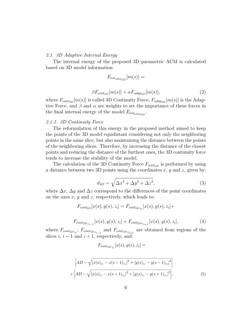
Figure 1 shows an example of the points and the distances involved inthe calculation of the force Fadap3D described by Eq. 4 taking a point Ci asa reference. This figure illustrates the distances used in Eq. 5 in green (slicei), and the ones in Eqs. 6 and 7 in red (slices i− 1 and i+ 1, respectively).

The resultant force Fcont3D uses the average distance between the pointsin the model (AD). This parameter is used as a target of the analyzeddistances, generating forces that increase the distances that are inferior to ADand reduce the distances that are superior to AD. Thus, the 3D continuitymodel force tends to make the connections between the model points equallyspaced in 3D. The average distance AD needs to be updated at each iteration,because when the points of the 3D model are moved, the distances betweenthem change. As result, this energy prevents that the points of the modelfrom moving uncoordinatedly not only in relation to the neighboring pointsin the same slice, but also in relation to the neighboring points in the slicesabove and below (Figure 1).

This strategy tends to improve the stability of the model.

2.1.2. 3D Adaptive Balloon Force

In the proposed method, the reformulation of this energy to 3D aimed tokeep the scope of the segmentation in different directions, but with an even

7

Figure 1: Illustration of the distances used to calculate the 3D Continuity Force, with thedistances used in Eq. 5 in green (slice i), and the distances used in Eqs. 6 and 7 in red(slices i− 1 and i+ 1, respectively).

faster rate than in the 2D method (Reboucas Filho et al., 2013; ReboucasFilho et al., 2014). This is possible by using information from neighboringslices to boost the movement of the model points.

The 3D Adaptive Balloon Force proposed in this work uses the topology ofeach point to move it, and takes into account the information of neighboringslices in the calculation of this force that will expand the model to 3D. Thus,this force must use the topology of 3 slices to move each point, increasingthe convergence of each point towards the object of interest. The quality ofinformation on the object of interest improves when the proposed model usesthree consecutive slices into account, i, i− 1 and i+1, where i is the slice ofthe point being analyzed.

Thus, the 3D Adaptive Balloon Force Fadap3D at a given point [c(s)] be-longing to the slice zi, whose coordinates are [x(s)zi , y(s)zi ], is given by:

Fadap3D [c(s), zi] = Fadap3Dzi[c(s), zi]+

Fadap3Dzi−1[c(s), zi] + Fadap3Dzi+1

[c(s), zi], (8)

8

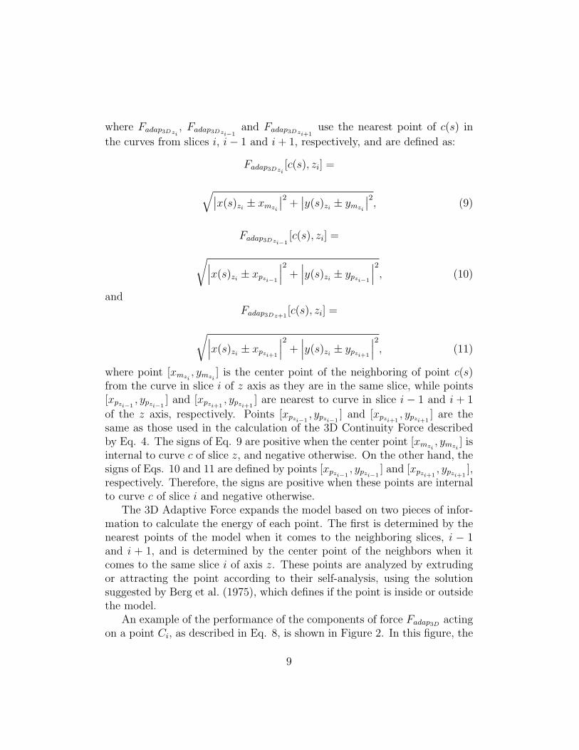
where Fadap3Dzi, Fadap3Dzi−1

and Fadap3Dzi+1use the nearest point of c(s) in

the curves from slices i, i− 1 and i+ 1, respectively, and are defined as:

Fadap3Dzi[c(s), zi] =

√∣∣x(s)zi ± xmzi

∣∣2 + ∣∣y(s)zi ± ymzi

∣∣2, (9)

Fadap3Dzi−1[c(s), zi] =√∣∣∣x(s)zi ± xpzi−1

∣∣∣2 + ∣∣∣y(s)zi ± ypzi−1

∣∣∣2, (10)

andFadap3Dz+1

[c(s), zi] =√∣∣∣x(s)zi ± xpzi+1

∣∣∣2 + ∣∣∣y(s)zi ± ypzi+1

∣∣∣2, (11)

where point [xmzi, ymzi

] is the center point of the neighboring of point c(s)from the curve in slice i of z axis as they are in the same slice, while points[xpzi−1


, ypzi+1] are nearest to curve in slice i − 1 and i + 1

of the z axis, respectively. Points [xpzi−1, ypzi−1

] and [xpzi+1, ypzi+1

] are thesame as those used in the calculation of the 3D Continuity Force describedby Eq. 4. The signs of Eq. 9 are positive when the center point [xmzi

, ymzi] is

internal to curve c of slice z, and negative otherwise. On the other hand, thesigns of Eqs. 10 and 11 are defined by points [xpzi−1


, ypzi+1],

respectively. Therefore, the signs are positive when these points are internalto curve c of slice i and negative otherwise.

The 3D Adaptive Force expands the model based on two pieces of infor-mation to calculate the energy of each point. The first is determined by thenearest points of the model when it comes to the neighboring slices, i − 1and i + 1, and is determined by the center point of the neighbors when itcomes to the same slice i of axis z. These points are analyzed by extrudingor attracting the point according to their self-analysis, using the solutionsuggested by Berg et al. (1975), which defines if the point is inside or outsidethe model.

An example of the performance of the components of force Fadap3D actingon a point Ci, as described in Eq. 8, is shown in Figure 2. In this figure, the

9

Figure 2: Illustration of the 3D Adaptive Balloon Force FMBiDi, FCi−1

and FCi+1from

slices i, i− 1 and i+ 1, respectively, where i is the position on axis z.

first component defined in Eq. 9 uses the center point of its neighbors MBiDi,

as shown in red in Figure 2. This is achieved by averaging its neighboringpoints Bi and Di. Analyzing this point by the Jordan Curve Theorem (Berget al., 1975), this point is taken as the internal point of the slice i, resultingin force FMBiDi

presented in yellow in Figure 2.The second and the third components of force Fadap3D are obtained from

the nearest points of the neighboring slices by Eqs. 10 and 11. Eq. 10defines the component from slice i − 1, using the point closest to point Ci

defined in Figure 2 as being point Ci−1. This point is analyzed based on theJordan Curve Theorem, Berg et al. (1975), changing the sign of Eq. 10 topositive, and pushing point Ci, as shown for force FCi−1

presented in green,so that it is inside the curve of slice i. Similarly, Eq. 11 uses point Ci+1

in the calculations so that this is the nearest to Ci in slice i + 1. In Figure2, this point is internal to the curve of slice i, changing the sign of Eq. 11to positive, which causes force FCi+1

, displayed in blue in Figure 2, to pushpoint Ci.

The movement of each point in the proposed 3D model is therefore influ-enced by the curves in the neighboring slices whilst in the 2D model, onlyslice i is analyzed by expanding the curve in this slice (Figure 2). Conse-

10

quently, the movement of each point of the 3D model towards the objects ofinterest resultant from the proposed energy is optimized as more informationis taken into account.

2.2. 3D Adaptive Crisp External Energy

The 3D Adaptive Crisp External Energy (3D ACEE) detects the originof the edges of the lungs based on the analysis of pulmonary densities inthe neighborhood of a voxel along with a Multi Layer Perceptron (MLP)artificial neural network to determining the origin of the edges found in the3D traditional external energy, which in this work is based on the Sobelgradient in 3D (Al-Dossary and Al-Garni, 2013).

Starting from the Analysis of Pulmonary Densities (APD) (ReboucasFilho et al., 2011) method performed in a 3D neighborhood of a voxel, thepercentages of 6 classes vi, in which i varies from 0 to 5, are: air hyper-inflated (1000 to 950 HU), normally air inflated (950 to 500 HU), low airinflated (500 to 100 HU), non-air inflated (100 to 100 HU), bone (600 to2000 HU) and areas not classified, which are the densities that do not fitin the previous ranges. From the definition of these classes, a CT lung isconsidered as a set of overlapping images, i.e. slices. This analysis T hasdimension l × c × a, where l × c is the dimension of the slices and a thenumber of slices of the exam under study.

Considering that the voxel under analysis has coordinates (x, y, z), thefunction that determines the number of voxels with densities present in eachclass vi is defined as:

f(x, y, z, vi) =n∑

l=−n

n∑m=−n

n∑o=−n

R(x− l, y −m, z − o), (12)

where n is the size of the analyzed neighborhood and R(x, y, z) is given by:

R(x, y, z) =

{1, liminf (vi) < T (x, y, z) < limsup(vi),0, otherwise,

(13)

where liminf (vi) and limsup(vi) are the lower and upper limits of the densityrange, in HU, for the class vi.

Using Eq. 12, it becomes possible to calculate the percentage Pi3D of eachclass i as:

Pi3D(x, y, z) =f(x, y, z, vi)4∑

j=0

f(x, y, z, vi)

. (14)

11

After exhaustive testing, it was concluded that by increasing n, the imagedetection quality is increased, because the neighborhood size is proportionalto n. However, a value of n above 7 increases the processing time consid-erably, without any significant improvements in the results. Therefore, thevalue 7 was used for n in the experiments.

The new 3D external energy uses an MLP artificial neural network inorder to determine the origin of each edge found in the CT scans of thethorax. This neural network has, as inputs, the percentage of each class vifound by the ADP method (Reboucas Filho et al., 2011), and a topology of6/4/1 (Reboucas Filho et al., 2013). Its output indicates if an edge foundin the thorax CT image belongs to the lung wall or not. Thus, a databaseis built from the voxel percentages extracted from examinations of COPD,cystic fibrosis and healthy patients.

A dataset was built manually, searching for the greatest possible rep-resentation of lung structures. Hence, 10 CT lung exams used as part ofdiagnostic investigations with approximately 5000 slices were analyzed. Thepercentage Pi3D was extracted for 500 voxels in each slice. Each set of in-puts for these percentages was labeled, indicating which of the edges foundin the 3D traditional external energy belonged to lung walls and which didnot. Emphasizing that the 3D traditional external energy was calculatedusing the Sobel 3D operator, which calculates an average of the gradientsfound throughout the neighborhood being analyzed. The dataset built wasvalidated by a cross-validation method (Haykin, 1999).

The following function is the output of the MLP network in execution,before its training phase:

fmlp3D(v) =

{1, edge similar to lung wall,0, otherwise,

(15)

where v consists of the 6 percentages Pi3D , where i varies from 0 to 5.Using fmlp3D in order to determine the origin of the edges found in the

CT lung images, the external energy is given by:

EextACEE3D(x, y, z) =

{Sobel3D(x, y, z), for fmlp3D (v) = 1,

1, otherwise, (16)

and v is the percentage vector of the ADP 3D method obtained from Eq. 12using coordinates (x, y, z) from the analyzed voxel.

Using Eq. 16, the MLP network determines the walls that are lung edgesor not returning the value 1 using the function fmlp3D . When this function

12

returns the value 0, it indicates that it is not a lung edge, and then theassociated region receives the maximum crisp adaptive energy. Small objectspresented only in a few number of slices now have less importance in the3D model than in the related 2D model, as the energy is calculated withinformation from multiple slices.

2.3. 3D Adaptive Crisp ACM Automatic Initialization

The 3D model automatically starts inside the lungs. The method deter-mines the initialization voxels in the right and left lungs, called 3D Right-hand initial voxels (RIP3D) and 3D Left-hand initial voxels (LIP3D), respec-tively. Each one of these voxels has coordinates (xini, yini, zini). To carry thisout, all the slices on the input CT scan are analyzed by the 2D initializationmethod in order to determine the exact initialization voxels (Reboucas Filhoet al., 2013). The values of the z coordinates of all slices that find a suc-cessful 2D automatic initialization are stored, then the average coordinate isadopted as zini and coordinates (xini, yini) obtained by the 2D method of thisslice are used as the initialization coordinates of voxels RIP3D and LIP3D.As such, the method tends to start in the center of each lung.

Figure 3 shows two curves presented in individual slices, where the dis-tance between each voxel, in red, from the center of the 3D model is givenby R; the blue line shows the centroid used in all slices and r is the radiusof the slice separated by a distance dz of the plane zini in the center of theslice I considering only the axis z.

Figure 3: Definition of the initialization parameters for the 3D model.

Figure 3 depicts that each slice has a different distance from the centroidfor each voxel. So, given slice zini that belongs to the center of the 3D model,it follows that the distance from the centroid for each voxel is the actual value.

13

When the curve is on another slice, value r must be calculated that is theradius of this further slice, and this value decreases as dz increases.

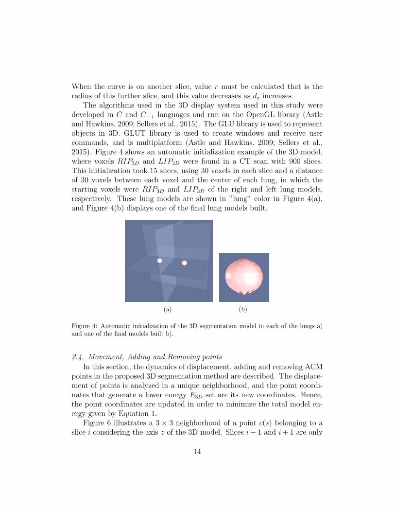
The algorithms used in the 3D display system used in this study weredeveloped in C and C++ languages and run on the OpenGL library (Astleand Hawkins, 2009; Sellers et al., 2015). The GLU library is used to representobjects in 3D. GLUT library is used to create windows and receive usercommands, and is multiplatform (Astle and Hawkins, 2009; Sellers et al.,2015). Figure 4 shows an automatic initialization example of the 3D model,where voxels RIP3D and LIP3D were found in a CT scan with 900 slices.This initialization took 15 slices, using 30 voxels in each slice and a distanceof 30 voxels between each voxel and the center of each lung, in which thestarting voxels were RIP3D and LIP3D of the right and left lung models,respectively. These lung models are shown in ”lung” color in Figure 4(a),and Figure 4(b) displays one of the final lung models built.

(a) (b)

Figure 4: Automatic initialization of the 3D segmentation model in each of the lungs a)and one of the final models built b).

2.4. Movement, Adding and Removing points

In this section, the dynamics of displacement, adding and removing ACMpoints in the proposed 3D segmentation method are described. The displace-ment of points is analyzed in a unique neighborhood, and the point coordi-nates that generate a lower energy E3D set are its new coordinates. Hence,the point coordinates are updated in order to minimize the total model en-ergy given by Equation 1.

Figure 6 illustrates a 3 × 3 neighborhood of a point c(s) belonging to aslice i considering the axis z of the 3D model. Slices i− 1 and i+ 1 are only

14

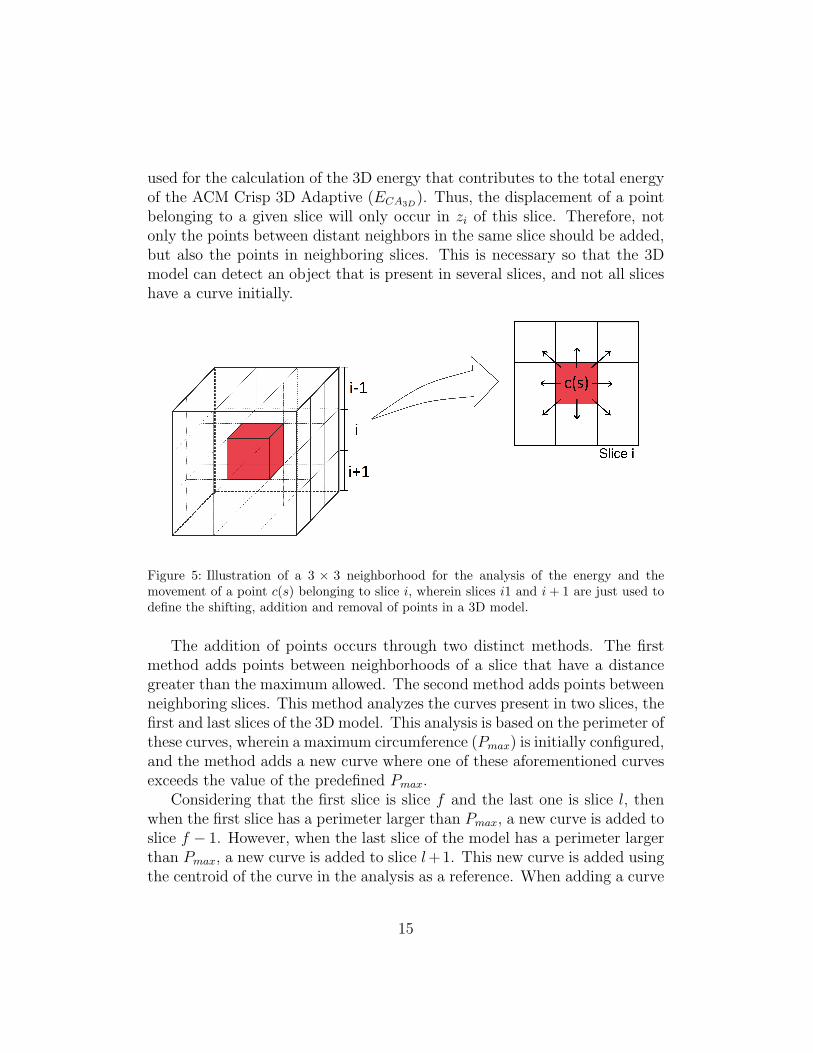
used for the calculation of the 3D energy that contributes to the total energyof the ACM Crisp 3D Adaptive (ECA3D

). Thus, the displacement of a pointbelonging to a given slice will only occur in zi of this slice. Therefore, notonly the points between distant neighbors in the same slice should be added,but also the points in neighboring slices. This is necessary so that the 3Dmodel can detect an object that is present in several slices, and not all sliceshave a curve initially.

Figure 5: Illustration of a 3 × 3 neighborhood for the analysis of the energy and themovement of a point c(s) belonging to slice i, wherein slices i1 and i+ 1 are just used todefine the shifting, addition and removal of points in a 3D model.

The addition of points occurs through two distinct methods. The firstmethod adds points between neighborhoods of a slice that have a distancegreater than the maximum allowed. The second method adds points betweenneighboring slices. This method analyzes the curves present in two slices, thefirst and last slices of the 3D model. This analysis is based on the perimeter ofthese curves, wherein a maximum circumference (Pmax) is initially configured,and the method adds a new curve where one of these aforementioned curvesexceeds the value of the predefined Pmax.

Considering that the first slice is slice f and the last one is slice l, thenwhen the first slice has a perimeter larger than Pmax, a new curve is added toslice f − 1. However, when the last slice of the model has a perimeter largerthan Pmax, a new curve is added to slice l+1. This new curve is added usingthe centroid of the curve in the analysis as a reference. When adding a curve

15

in slice f − 1 it is used the centroid of f and when adding a curve to slicel + 1 the centroid of the curve from slice l is used.

Figure 6 illustrates the application of this method using 30 as the max-imum perimeter Pmax and the initialization parameters assuming the value10 as the distance from each point to the centroid and 30 as the number ofvertices. In Figure 6(a), the upper and lower slices have greater perimetersthan Pmax; Figure Figure 6(b) shows the visualization of this model with aninternal view of the top slice. The results of applying the points additionmethod in the upper and lower slices are shown in Figure 6(c). Figure 6(d)shows the external and internal views of the model, respectively, after theaddition of the points.

(a) (b)

(c) (d)

Figure 6: Adding slices to a 3D model: a) 3D model with areas larger than the onesdefined in the first and last slices; b) top view of the model in a); c) 3D model after addingthe new slices; and d) top view of the model in c).

Another important step in the proposed method is the removal of pointsfrom the 3D model. Analogously to the method of addition of points, this

16

step is also based on two methods. The first method uses information of theneighbors of a point in the same slice as illustrated in Figure 7. The angleformed between the analyzed point and its neighbors in this slice is calculated

as α = arccos(

a2+b2−c2

2bc

), and if this angle is less than a predefined angle, this

point is removed from the model and model is reordered. In summary thismethod removes the model points that are misaligned with their neighbors.

Figure 7: Calculation of the angle between a point and its neighbors on the same slice.

The second method follows the same principle to remove points fromits neighbors, but expanding the principle to 3D. This is possible using theclosest points in neighboring slices. Thus, considering a point belonging toslice zi, the nearest point of slice zi−1 and the closest point of slice zi+1 used,as illustrated in Figure 8 with points Ci, Ci−1 and Ci+1 belonging to slices i,i− 1 and i+ 1, respectively.

The analysis for the removal of points is based on the angle formed be-tween the neighbor points that is compared with a predefined minimum angleθmin. An analyzed point is removed when the angle between the point andthe closest ones in the neighboring slices is less than θmin. Given the modelshown in Figure 8, one can see the point Ci forming an angle θ with Ci−1 andCi+1, where these are the closest points in slices i− 1 and i+1, respectively.

Angle θ1 shown in Figure 8(a) is greater than angle θ2 in Figure 8(b). Thisis because Ci is less aligned with Ci−1 and Ci+1 in the formation of θ2, whichdoes not occur in the formation of θ1. The angle θ formed between a point and

its closest points in the neighboring slices is given by θ = arccos(

a2+b2−c2

2bc

),

where a, b and c are the parameters identified in Figure 8.Thus, the removal methods tend to exclude the misaligned points from

17

(a)

(b)

Figure 8: Illustration of the parameters used for calculating the angles formed betweena point of slice i with its nearest neighbor in slices i − 1 and i + 1: a) and b) show thedefinition of angles θ1 and θ2, respectively.

the other slices. The points removed are points that are misalignment relativeto their neighbors in the same slice or relative to the points in curves presentin the neighboring slices. This makes the model smoother and avoids grosserrors in the 3D segmentation.

2.5. Automatic Segmentation of Lungs in Thorax CT Scans

The automatic segmentation of the lungs in a CT scan of the thorax usesthe methods previously described for the automatic initialization of the 3Dmodel, addition and removal of points and the 3D Adaptive Crisp ACM. The

18

Figure 9:Flowchart for implementing the 3D Adaptive Crisp ACM.

methods are executed according to the flowchart shown in Figure 9, whichalso includes examples related to each step involved.

19

The first step in segmenting the lungs automatically in a CT examina-tion is to open all the DICOM images. To carry this out, the free libraryDCMTK is used to read the image and its parameters and to identify andorder the CT scan slices. Then, the whole external energy is calculated usingthe 3D Adaptive Crisp method for detecting the origin of the edges obtainedby the 3D traditional external energy. The edges detected inside the lungsare excluded from the external energy. The centroid of the 3D model withcoordinates xini, yini and zini is determined by the slice of the average co-ordinate zi, considering all slices i, where the lung was found using the 2Dmethod suggested in Reboucas Filho et al. (2013). The 3D model undergoes successive iterations of the 3D Adaptive Crisp ACM method in orderto decrease the energy of the model by moving its points. In each of theiterations, the methods of 3D points removal and addition are applied.

(a) (b) (c)

(d) (e) (f)

Figure 10: Lung segmentation in CT scans by 3D Adaptive Crisp ACM: a) automaticinitialization of the 3D model; b) to e), evolution of the 3D model, and f) final result.

The model is stable when the volume does not increase after two con-secutive iterations. When this happens, the segmentation of the lung iscomplete. Figure 10 shows an example of a segmentation obtained by theproposed method, from the initialization to the stabilization of the 3D model.

20

2.6. Statistical measures

In order to analyze the segmentation performance, three well-known mea-sures were employed: recall, precision and F-measure, whose definitions arebriefly described here:

Recall (aka Sensitivity) is the ratio between the number of correctly seg-mented voxels of a given class and the total number of voxels in the CT scanof the thorax under analysis, including those that were incorrectly segmented:

Recall =true positives

true positives + false negatives, (17)

where true positives and false negatives stand for the number of voxels of agiven class correctly and incorrectly segmented, respectively.

Precision (aka Positive predictive value) means the ratio between thenumber of correctly segmented voxels of a specific class and the total numberof voxels in the CT scan of the thorax under analysis as belonging to thatclass:

precision =true positives

true positives + false positives, (18)

where true positives and false positives denote the number of voxels correctlyand incorrectly segmented as belonging to the considered class, respectively.

The F-measure (Fm) for a given class is calculated as the harmonic meanof the Recall and precision values for that specific class, resulting in a moreglobal parameter for evaluating the performance of a classifier on each class.More formally:

Fm = 2

(Recall × precision

Recall + precision

). (19)

3. Experimental Results

In this section, we present the results in terms of computational cost andperformance of each lung segmentation method under comparison. The testswere performed on a notebook with an Intel Core i5 1.4 GHz, 4 GB of RAM,and running MAC OS X 10.10.5.

In the evaluation, the computational cost (processing time), positive pre-dictive value (precision), sensitivity (recall) and F-measure were used to cal-culate the similarity between the shapes under comparison.

21

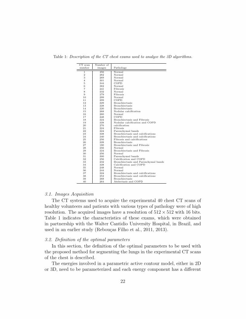
Table 1: Description of the CT chest exams used to analyze the 3D algorithms.

CT scan Number ofnumber images Pathology

1 456 Normal2 282 Normal3 269 Normal4 301 Normal5 344 COPD6 382 Normal7 241 Fibrosis8 232 Normal9 279 Fibrosis10 299 Normal11 299 COPD12 229 Bronchiectasis13 228 Bronchiectasis14 220 Bronchiectasis15 268 Nodular calcification16 260 Normal17 248 COPD18 224 Bronchiectasis and Fibrosis19 228 Nodular calcification and COPD20 276 calcification21 224 Fibrosis22 224 Parenchymal bands23 228 Bronchiectasis and calcifications24 240 Bronchiectasis and calcifications25 256 Fibrosis and calcifications26 228 Bronchiectasis27 180 Bronchiectasis and Fibrosis28 256 Normal29 224 Bronchiectasis and Fibrosis30 256 Normal31 300 Parenchymal bands32 256 Calcification and COPD33 232 Bronchiectasis and Parenchymal bands34 228 Calcification and COPD35 248 Normal36 244 Normal37 224 Bronchiectasis and calcifications38 252 Bronchiectasis and calcifications39 268 Bronchiectasis40 264 Atelectasis and COPD

3.1. Images Acquisition

The CT systems used to acquire the experimental 40 chest CT scans ofhealthy volunteers and patients with various types of pathology were of highresolution. The acquired images have a resolution of 512× 512 with 16 bits.Table 1 indicates the characteristics of these exams, which were obtainedin partnership with the Walter Cantidio University Hospital, in Brazil, andused in an earlier study (Reboucas Filho et al., 2011, 2013).

3.2. Definition of the optimal parameters

In this section, the definition of the optimal parameters to be used withthe proposed method for segmenting the lungs in the experimental CT scansof the chest is described.

The energies involved in a parametric active contour model, either in 2Dor 3D, need to be parameterized and each energy component has a different

22

importance in the calculation of the total energy for each pixel or voxel.As such, the parameters α, β and τ define the weights of the 3D AdaptiveBalloon Force, 3D Continuity Force and 3D Adaptive Crisp External energy,respectively, in the calculation of the total energy.

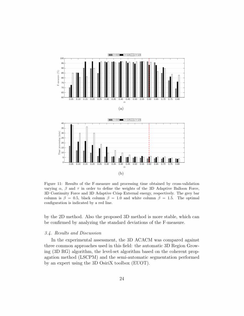
The optimal parameters were defined by cross-validation varying eachparameter and considering the sum of all as equal to 1 (one). The graphs ofFigure 11 depict the results of the F-measures and processing times. Threecolumns are shown for three different weights for 3D Continuity Force, thegray column is β = 0.5, black column β = 1.0 and white column β = 1.5. Thex-axis shows the values of parameter α and the τ value is the complement ofthe sum between α and β to 1 (τ = 1− α− β). These results were obtainedusing 6 CT scans considering different clinical cases: normal (CT scans 1and 4), calcification (CT scans 15 and 20), bronchiectasis (CT scan 26), andparenchymal bands (CT scan 31).

Analyzing Figure 11(a), one can verify that if alpha is increased, theF-measure value will increase until it stabilizes; yet, it starts to drop fromα = 0.5. However, analyzing Figure 11(b), one can see that the higherthe alpha value is, the faster the lung segmentation in CT scans tends tobe. Therefore, the optimal configuration was obtained using β = 0.05 (greycolumn) with α = 0.60, and τ = 0.35, as indicated by the red line shown inFigure 11. This option will lead to the shortest possible processing time andhighest efficiency.

3.3. Numerical contribution of the proposed 3D method compared to the 2Dmethod

To evaluate numerically the contribution of the proposed 3D methodcompared to the 2D method proposed in Reboucas Filho et al. (2013), we usedthe optimal configuration obtained for both methods on the same 6 CT scans(Figure 11). The 2D method obtained an F-measure of 96.33% ± 0.42 anda processing time of 12.52± 2.10 minutes. The proposed 3D Adaptive CrispActive Contour obtained an F-measure of 99.14%±0.18 and a processing timeof 3.20± 0.38 minutes. These results demonstrate that the novel 3D energyaccelerates the convergence of the 3D model, thus reducing the processingtime, with the combination of each new 3D energy making the proposed 3Dmethod 3.91 times faster than the 2D method compared under the sameexperimental settings and conditions.

The use of the Sobel 3D operator resulted in the F-measure average valueobtained by the proposed 3D model being 3.5% higher than the one obtained

23

α0.05 0.10 0.15 0.20 0.25 0.30 0.35 0.40 0.45 0.50 0.55 0.60 0.65 0.70 0.75 0.80

F-m

easure

(%)

60

65

70

75

80

85

90

95

100

β = 0.5 β = 1.0 β = 1.5

(a)

α0.05 0.10 0.15 0.20 0.25 0.30 0.35 0.40 0.45 0.50 0.55 0.60 0.65 0.70 0.75 0.80

Tim

eprocessing(m

in)

0

5

10

15

20

25

30

35

40

β = 0.5 β = 1.0 β = 1.5

(b)

Figure 11: Results of the F-measure and processing time obtained by cross-validationvarying α, β and τ in order to define the weights of the 3D Adaptive Balloon Force,3D Continuity Force and 3D Adaptive Crisp External energy, respectively. The grey barcolumn is β = 0.5, black column β = 1.0 and white column β = 1.5. The optimalconfiguration is indicated by a red line.

by the 2D method. Also the proposed 3D method is more stable, which canbe confirmed by analyzing the standard deviations of the F-measure.

3.4. Results and Discussion

In the experimental assessment, the 3D ACACM was compared againstthree common approaches used in this field: the automatic 3D Region Grow-ing (3D RG) algorithm, the level-set algorithm based on the coherent prop-agation method (LSCPM) and the semi-automatic segmentation performedby an expert using the 3D OsiriX toolbox (EUOT).

24

The 3D Adaptive Crisp ACM method was configured with the parame-ters (as described in Section 3.2) α = 0.60, β = 0.05 and τ = 0.35 in thecalculation of the total energy. After the initialization, the centroids weredetermined. To build the initial 3D model, 30 voxels per slice with a radiusvalue of 50 voxels for the distance to the centroid were used. The maxi-mum distance d among voxels considered in the addition of new voxels wasequal to 5 voxels and the minimum angle between a voxel and its neighborsconsidered in the removal of voxels was defined as 45 degrees.

The 3D RG algorithm used the same initialization as 3D Adaptive CrispACM, with the entire internal region of the ACM initialization polygon usedas seed. The neighboring regions addition method uses lung anatomy in-formation, only adding voxels that are on intensity edges within the lung,which are: normally aerated, slightly aerated or hyper-inflated. This ad-dition occurs by successive iterations, ending when no more voxels can beadded. Two updates are made in this method. First of all, the trachea andthe hilum are targeted separately by removing the voxels of this region fromthe result of the segmentation of the lungs. Finally, if the regions of bothlungs are tending to merge, the frontier between the two lungs is updated toavoid segmenting regions of one lung as of the other lung. This frontier ismoved to the location of the smallest diameter between the regions. Assum-ing that the voxels where the two lungs merge looks like an hourglass, thefrontier is moved to the middle of the hourglass.

There are several types of commercial medical software with plugins andtoolboxes that can be used to compare the proposed method. We used onethat is mostly used in hospitals and also in recent researches. Hence, the level-set algorithm based on the coherent propagation method (LSCPM), proposedby Wang et al. (2011, 2014), was used in this work for lung segmentation viathe MIA plugin for OsiriX (http://www.mia-solution.com).

Another segmentation approach possible is the semi-automatic segmenta-tion by an expert using the 3D OsiriX toolbox (EUOT). In this approach, theexpert visualizes the 3D objects presented in the input exam, and removesundesired objects (Michael P Chae, 2015). The use of EUOT is in fact widelyadopted by many doctors; however, this tool is based on simple segmentationtechniques such as thresholding and region growing. Thus, when the lungunder analysis has some disease, manual corrections should be made in eachslice of the CT dataset; however, this tool does not allow this straightforwardprocedure. Figure 12 shows examples of the segmentations obtained by themethods under comparison.

25

http://www.mia-solution.com

(a) (b) (c)

(d) (e) (f)

(g) (h) (i)

(j) (k) (l)

Figure 12: Lung segmentation in CT scans by the methods under comparison: a), b)and c) 3D Adaptive Crisp ACM; d), e) and f) 3D Region Growing; g), h) and i) Level-set algorithm based on the coherent propagation method; j), k) and l) semi-automaticsegmentation by an expert using the 3D OsiriX toolbox.

26

The segmentations obtained by each method under comparison were eval-uated using 40 CT scans of the chest. Each CT scan was assessed along itslength from the apex to the base of the lung, removing one in eight slices.

The segmentations used as ground truth were built semi-automaticallyusing commercial software and manual corrections were subsequently carriedout by a medical expert on the existing errors.

Table 2 shows the statistical results obtained for the 40 CT scans in termsof healthy patients and patients with diseases. In the case of the diseasedCT scans, there are two groups, the first group with decreased HU density insome regions of the lung such as those due to COPD and bronchiectasis, andthe second group with increased HU densities such as those due to fibrosis,calcification and atelectasis.

Table 2: Statistical analysis of the F-measure (FM) values obtained for the lung segmen-tation methods on the experimental CT scans in terms of healthy lungs (HL), lungs withdisease that increase or decrease the HY density (DID and DDD, respectively), and globalresults (GR).

Segm.Method

Right lung Left lung Both lungsFM(%) FM(%) FM(%) Time(min)

HL

3D ACACM 99.93±0.19 98.82±0.22 99.22±0.14 3.54±0.793D RG 98.19±0.74 98.28±0.77 98.57±0.54 2.51±0.55EUOT 98.03±1.16 97.92±1.27 98.53±0.99 4.38±0.89LSCPM 98.26±1.25 98.08±1.36 98.73±1.04 1.18±0.26

DDD


DID


GR


This study adopted the F-measure as the quality metric because thismeasure takes into account only the lung region in the calculations. Manyauthors use the accuracy as an evaluation metric, but in this case, this metricdoes not lead to accurate results, since the lung is just a small part of the totalimaged volume, and accuracy considers the whole volume under examination,

27

which can lead to erroneous analysis of the results.Regarding the results presented in Table 2, there are four analyzes. The

first one evaluates healthy patients, and here the average F-measure by theproposed method is better for both lungs with a value of 99.22%± 0.14, fol-lowed by the Level-set algorithm based on the coherent propagation methodwith a value of 98.73%±1.04 for this metric, then the 3D RG with 98.57%±0.54 and finally, the semi-automatic segmentation by an expert using 3DOsiriX toolbox with 98.53%± 0.99.

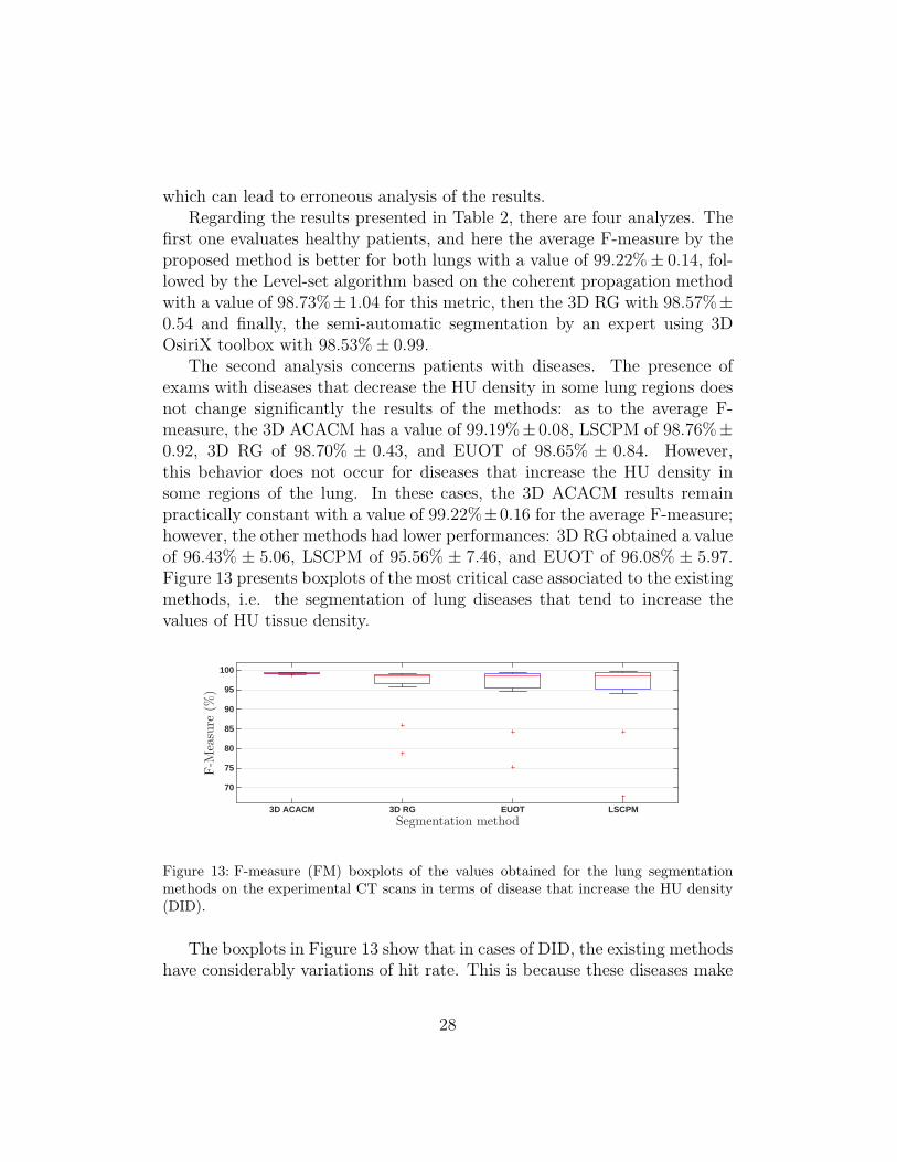
The second analysis concerns patients with diseases. The presence ofexams with diseases that decrease the HU density in some lung regions doesnot change significantly the results of the methods: as to the average F-measure, the 3D ACACM has a value of 99.19%±0.08, LSCPM of 98.76%±0.92, 3D RG of 98.70% ± 0.43, and EUOT of 98.65% ± 0.84. However,this behavior does not occur for diseases that increase the HU density insome regions of the lung. In these cases, the 3D ACACM results remainpractically constant with a value of 99.22%±0.16 for the average F-measure;however, the other methods had lower performances: 3D RG obtained a valueof 96.43% ± 5.06, LSCPM of 95.56% ± 7.46, and EUOT of 96.08% ± 5.97.Figure 13 presents boxplots of the most critical case associated to the existingmethods, i.e. the segmentation of lung diseases that tend to increase thevalues of HU tissue density.

Segmentation method3D ACACM 3D RG EUOT LSCPM

F-M

easure

(%)

70

75

80

85

90

95

100

Figure 13: F-measure (FM) boxplots of the values obtained for the lung segmentationmethods on the experimental CT scans in terms of disease that increase the HU density(DID).

The boxplots in Figure 13 show that in cases of DID, the existing methodshave considerably variations of hit rate. This is because these diseases make

28

the unhealthy lung tissue very dissimilar to healthy lung tissue. However, theproposed method remains robust with an almost constant hit rate, obtainingresults similar for healthy volunteers and patients with DDD and DID.

Figure 14 shows the results considering healthy and unhealthy lungs andillustrates common errors that can occur in this field. The results are pre-sented according to the following: the first row shows healthy lungs; thesecond row shows lungs with COPD; the third row presents lungs withBronchiectasis and Parenchymal bands; the fourth row shows lungs withBronchiectasis and Fibrosis; the fifth row shows lungs with Nodular calci-fication and COPD. The results are presented with true positives in green,false negatives in red, and false positives in orange and blue (blue is used inthe cases where the border between the 2 lungs is unclear), and the originalgrayscale represents true negatives.

Regarding Figure 14, the results in the first row indicate that all meth-ods obtained correct segmentations. The slices in the third, fourth and fifthrows, are associated to lung diseases that increase the HU density whichconfounds inside lung regions with outer lung regions. The methods com-pared against the proposed 3D ACACM method had lower performance insegmenting these slices. Instead, the proposed method had a stable per-formance in all of these cases due to its external energy and integration ofartificial intelligence that enhances its performance even more. The internalenergy makes segmentation of objects with different shapes possible, buildingthe correct 3D segmented model due to its integration with the appropriateexternal force.

In the fifth row of Figure 14, there are small blue regions in the results ob-tained by the existing methods, meaning an uncertainty of where the borderbetween the two lungs is; however, the proposed method performed very wellalso due to the adopted external energy. Furthermore, the proposed internalenergy becomes more regular and stable in the 3D model and thus reducesgross segmentation errors. Note that this behavior of the 3D ACACM energycan also cause minor errors, as shown in yellow in these slices, because the3D model is more stable and therefore, very small objects presented in a fewslices may be ignored, such as blood vessels and internal lung airways.

The last analysis is the global analysis that reflects the same observationsof the previous analysis: the proposed method obtained an average F-measureof 99.22% ± 0.14, 3D RG of 97.59% ± 3.67, EUOT of 97.39% ± 4.35, andLSCPM of 97.22% ± 5.43. Thus, one can say that the current methodsunder comparison attained average F-measure values higher that 98.5% in the

29

(a) (b) (c) (d) (e)

(f) (g) (h) (i) (j)

(k) (l) (m) (n) (o)

(p) (q) (r) (s) (t)

(u) (v) (w) (x) (y)

Figure 14: Examples of lung segmentations in CT scans obtained by the different methodsunder evaluation: a), f), k), p), u) original images; b), g), l), q) and v) 3D AdaptiveCrisp ACM; c), h), m), r) and w) 3D Region Growing; d), i), n), s) and x) Level-setalgorithm based on the coherent propagation method; and e), j), o), t) and y) semi-automatic segmentation by expert using the 3D OsiriX toolbox.

30

healthy patients and in the patients with diseases that tend to diminish theHU density in some lung regions. However, the proposed method was morestable and obtained an average F-measure over 99% in all tests independentlyof the type of disease presented.

Regarding the segmentation time, the most efficient methods in ascendingorder were the Level-set algorithm based on the coherent propagation methodwith 1.03 ± 0.19 minutes, 3D RG with 2.20 ± 0.40 minutes, 3D ACACMwith 3.11±0.57 minutes, and the semi-automatic segmentation by an expertusing the 3D OsiriX toolbox with 3.89±0.66 minutes. The proposed methodobtained an average result of 3 minutes, which is three times the time requiredby the automatic commercial plugin software used to build the ground truthand 1.5 times of the 3D RG time. However, the 3D ACACM is eight timesfaster than the expert, which took 25 minutes on average in using the semi-automated commercial software with subsequent manual improvements.

The experimental dataset used and the results obtained are available athttp://lapisco.ifce.edu.br/?page id=131.

4. Conclusion

This work proposes a method called 3D Adaptive Crisp that is a newtechnique of automatic segmentation of lungs in CT scans of the thorax. Themain contributions achieved by the proposed method are related to the new3D Adaptive Crisp external energy, the novel 3D Adaptive Balloon internalenergy and the robust 3D automatic initialization.

As secondary contributions, but also important to the quality of the re-sults obtained, are the developed solutions for the addition, removal andinitialization of points, which were not successfully overcome by previousstudies. The use of the Sobel 3D operator allows better analysis of theobjects present in the input image dataset through the proposed external en-ergy. These contributions give a parametric method of active contour, suchas Snakes, the ability to have results similar to the ones obtained by geo-metrical methods of active contours, such as Level Set, even when comparedagainst an optimized Level-Set algorithm.

The 3D Adaptive Crisp was compared against three methods commonlyused by specialists in the segmentation of CT scans of the thorax both fromhealthy and diseased patients, using a ground truth built by a medical expert.

The proposed method was comparatively more stable than the othermethods independently of the diseased presented, obtaining an average F-

31

http://lapisco.ifce.edu.br/?page_id=131

measure over 99% in all tests. The findings confirmed that the proposedmethod is superior to the other methods under comparison, and its suit-ability to be used in clinical routine diagnosis, since it requires less than 4minutes to accomplish the segmentation in a common personal computer.

As to future works, we intend to apply other computational intelligenceand pattern recognition techniques to identify the origin of edges found in thelungs, to adapt the methods developed for the detection of other organs, andto investigate methods for the recognition of lung or other organ diseases.

Acknowledgements

Pedro P. Reboucas Filho acknowledges the sponsorship from the Fed-eral Institute of Education, Science and Technology of Ceara, in Brazil, viaGrants PROINFRA-IFCE/2013 and PROAPP-IFCE/2014. He also acknowl-edges the sponsorship from the Brazilian National Council for Research andDevelopment (CNPq) through Grant 232644/2014-4.

Victor Hugo C. de Albuquerque acknowledges the sponsorship from theBrazilian National Council for Research and Development (CNPq) via Grants470501/2013-8 and 301928/2014-2.

Joao Manuel R. S. Tavares thanks the funding of Project NORTE-01-0145-FEDER-000022 - SciTech - Science and Technology for Competitiveand Sustainable Industries, co-financed by “Programa Operacional Regionaldo Norte” (NORTE2020), through “Fundo Europeu de Desenvolvimento Re-gional” (FEDER).

References

Al-Dossary, S., Al-Garni, K., 2013. New parametric 3d snake for medicalsegmentation of structures with cylindrical topology, in: SPE Saudi ArabiaSection Technical Symposium and Exhibition, pp. 276–280.

Ariani, A., Carotti, M., Gutierrez, M., Bichisecchi, E., Grassi, W., Giusep-petti, G., Salaffi, F., 2014. Utility of an open-source dicom viewer software(OsiriX) to assess pulmonary fibrosis in systemic sclerosis: preliminaryresults. Rheumatology International 34, 511–516.

Arunkumar, R., 2012. Quantitative analysis of bronchiectasis using localbinary pattern and fuzzy based spatial proximity, in: Recent Trends In

32

Information Technology (ICRTIT), 2012 International Conference on, pp.72–76.

Astle, D., Hawkins, K., 2009. Begnning OpenGl Game Programming. Thom-son, EUA. 2nd edition.

Berg, G., Julian, W., Mines, R., Richman, F., 1975. The constructive jordancurve theorem. Journal of Mathematics 5, 225–236.

Born, S., Dirkiwamaru, Pfeile, M., Bartz, D., 2009. 3-step segmentation ofthe lower airways with advanced leakage-control. IJCAI-09 workshop onExplanation-aware Computing (ExaCt 2009) , 239–255.

Campos, H., Lemos, A., 2009. Asthma and copd in view of the pulmonologist.Brazilian Journal of Pulmonology 35, 301–309.

Canas, S., Leehan, J., Jimenez-Alaniz, J., 2007. Plugin for OsiriX: Meanshift segmentation, in: Engineering in Medicine and Biology Society, 2007.EMBS 2007. 29th Annual International Conference of the IEEE, pp. 3060–3063.

De Nunzio, G., Tommasi, E., Agrusti, A., Cataldo, R., De Mitri, I., Favetta,M., Maglio, S., Massafra, A., Quarta, M., Torsello, M., Zecca, I., Bellotti,R., Tangaro, S., Calvini, P., Camarlinghi, N., Falaschi, F., Cerello, P.,Oliva, P., 2011. Automatic lung segmentation in ct images with accuratehandling of the hilar region. Journal of Digital Imaging 24, 11–27.

Diciotti, S., Lombardo, S., Falchini, M., Picozzi, G., Mascalchi, M., 2011.Automated segmentation refinement of small lung nodules in CT scans bylocal shape analysis. IEEE Transactions on Biomedical Engineering 58,3418–3428.

Ge, Q., Shen, F., Jing, X.Y., Wu, F., Xie, S.P., Yue, D., Li, H.B., 2016.Active contour evolved by joint probability classification on riemannianmanifold. Signal, Image and Video Processing , 1–8.

Hame, Y., Angelini, E., Hoffman, E., Barr, R., Laine, A., 2014. Adaptivequantification and longitudinal analysis of pulmonary emphysema witha hidden Markov measure field model. IEEE Transactions on MedicalImaging 33, 1527–1540.

33

Haykin, S., 1999. Neural Networks: A Comprehensive Foundation. Prentice-Hall, EUA. 2nd edition.

Irving, B., TaylorR, P., Todd-Pokropek, A., 2009. 3D segmentation of theairway tree using a morphology based method. IJCAI-09 workshop onExplanation-aware Computing (ExaCt 2009) , 297–307.

Juen, J., Cheng, Q., Schatz, B., 2015. A natural walking monitor for pul-monary patients using mobile phones. IEEE Journal of Biomedical andHealth Informatics 19, 1399–1405.

Korfiatis, P., Kalogeropoulou, C., Karahaliou, A., Kazantzi, A., Costaridou,L., 2011. Vessel tree segmentation in presence of interstitial lung diseasein MDCT. Information Technology in Biomedicine, IEEE Transactions on15, 214–220.

Kwan, A., Fung, A., Jansen, P., Schivo, M., Kenyon, N., Delplanque, J.P.,Davis, C., 2015. Personal lung function monitoring devices for asthmapatients. IEEE Sensors Journal 15, 2238–2247.

Leninisha, S., Vani, K., 2015. Water flow based geometric active deformablemodel for road network. ISPRS Journal of Photogrammetry and RemoteSensing 102, 140 – 147.

Lo, P., van Ginneken, B., Reinhardt, J., Yavarna, T., Jong, P., Irving, B.,Fetita, C., Ortner, M., Pinho, R., Sijbers, J., Feuerstein, M., Fabijanska,A., Bauer, C., Beichel, R., Mendoza, C., Wiemker, R., Lee, J., Reeves,A., Born, S., Weinheimer, O., van Rikxoort, E., Tschirren, J., Mori, K.,Odry, B., Naidich, D., Hartmann, I., Hoffman, E., Prokop, M., Pedersen,J., Bruijne, M., 2012. Extraction of airways from CT (EXACT’09). IEEETransactions on Medical Imaging 31, 2093–2107.

Mansoor, A., Bagci, U., Xu, Z., Foster, B., Olivier, K., Elinoff, J., Suffredini,A., Udupa, J., Mollura, D., 2014. A generic approach to pathological lungsegmentation. IEEE Transactions on Medical Imaging 33, 2293–2310.

Marco, R., Accordini, S., Cerveri, I., Corsico, A., Sunyer, J., Neukirch, F.,Kunzly, N., Leynaert, B., Janson, C., Gislason, T., Vermeire, P., Svanes,C., Anto, J., Burney, P., 2004. An international survey of chronic obstru-tive pulmonary disease in young adults according to gold stages. Thorax59, 120–125.

34

Martin, C.M., Roach, V.A., Nguyen, N., Rice, C.L., Wilson, T.D., 2013.Comparison of 3d reconstructive technologies used for morphometric re-search and the translation of knowledge using a decision matrix. Anatom-ical Sciences Education 6, 393–403.

Matsuoka, S., Yamashiro, T., Washko, G., Kurihara, Y., 2010. QuantitativeCT assessment of chronic obstructive pulmonary disease. RadioGraphics30, 55–66.

Mesejo, P., Valsecchi, A., Marrakchi-Kacem, L., Cagnoni, S., Damas, S.,2015. Biomedical image segmentation using geometric deformable modelsand metaheuristics. Computerized Medical Imaging and Graphics 43, 167– 178.

Michael P Chae, David J Hunter-Smith, A.R.R.T.S.W.M.R., 2015. 3d vol-umetric analysis and haptic modeling for preoperative planning in breastreconstruction. Anaplastology 4, –.

Mieloszyk, R., Verghese, G., Deitch, K., Cooney, B., Khalid, A., Mirre-Gonzalez, M., Heldt, T., Krauss, B., 2014. Automated quantitative analy-sis of capnogram shape for copd normal and copd chf classification. IEEETransactions on Biomedical Engineering 61, 2882–2890.

Moallem, P., Tahvilian, H., Monadjemi, S.A., 2015. Parametric active con-tour model using gabor balloon energy for texture segmentation. Signal,Image and Video Processing 10, 351–358.

Moreira, F.D.L., Kleinberg, M.N., Arruda, H.F., Freitas, F.N.C., Parente,M.M.V., de Albuquerque, V.H.C., Filho, P.P.R., 2016. A novel vickershardness measurement technique based on adaptive balloon active contourmethod. Expert Systems with Applications 45, 294 – 306.

Nemec, S., Molinari, F., Dufresne, V., Gosset, N., Silva, M., Bankier, A.,2015. Comparison of four software packages for CT lung volumetry inhealthy individuals. European Radiology 25, 1588–1597.

Presti, G., Carbone, M., Ciriaci, D., Aramini, D., Ferrari, M., Ferrari, V.,2015. Assessment of dicom viewers capable of loading patient-specific3d models obtained by different segmentation platforms in the operatingroom. Journal of Digital Imaging 28, 518–527.

35

Pu, J., Fuhrman, C., Good, W., Sciurba, F., Gur, D., 2011. A differential ge-ometric approach to automated segmentation of human airway tree. IEEETransactions on Medical Imaging 30, 266–278.

Qiu, W., Yuan, J., Rajchl, M., Kishimoto, J., Chen, Y., de Ribaupierre, S.,Chiu, B., Fenster, A., 2015. 3d MR ventricle segmentation in pre-terminfants with post-hemorrhagic ventricle dilatation (PHVD) using multi-phase geodesic level-sets. NeuroImage 118, 13 – 25.

Ramalho, G.L.B., Reboucas Filho, P.P., Medeiros, F.N.S., Cortez, P.C., 2014.Lung disease detection using feature extraction and extreme learning ma-chine. Research on Biomedical Engineering 30, 207 – 214.

Reboucas, E.S., Braga, A.M., Marques, R.C., Filho, P.P.R., 2016. A newapproach to calculate the nodule density of ductile cast iron graphite usinga level set. Measurement 89, 316 – 321.

Reboucas Filho, P.P., Cortez, P.C., Felix, J.H.S., T. S. Cavalcante, T.d.S.,Holanda, M.A., 2013. Adaptive 2D crisp active contour model applied tolung segmentation in CT images of the thorax of healthy volunteers andpatients with pulmonary emphysema,. Research on Biomedical Engineer-ing 29, 363–376.

Reboucas Filho, P.P., Cortez, P.C., Holanda, M.A., 2011. Active contourmodes crisp: new technique for segmentation the lungs in CT images.Research on Biomedical Engineering 27, 259–272.

Reboucas Filho, P.P., Cortez, P.C., da Silva Barros, A.C., Albuquerque,V.H.C., 2014. Novel adaptive balloon active contour method based oninternal force for image segmentation a systematic evaluation on syntheticand real images. Expert Systems with Applications 41, 7707 – 7721.

Schmitter, D., Gaudet-Blavignac, C., Piccini, D., Unser, M., 2015. Faultdetection and characterization using a 3d multidirectional sobel filter, in:2015 IEEE International Conference on Image Processing (ICIP), pp. 276–280.

Sellers, G., Junior, R.W., Haemel, N., 2015. OpenGL Superbible: Compre-hensive tutorial and reference. Addison-Wesley, EUA. 7th edition.

36

Sorensen, L., Nielsen, M., Lo, P., Ashraf, H., Pedersen, J., Bruijne, M.,2012. Texture-based analysis of copd: A data-driven approach. IEEETransactions on Medical Imaging 31, 70–78.

Spina, G., Casale, P., Albert, P., Alison, J., Garcia-Aymerich, J., Costello,R., Hernandes, N., van Gestel, A., Leuppi, J., Mesquita, R., Singh, S.,Smeenk, F., Tal-Singer, R., Wouters, E., Spruit, M., den Brinker, A., 2015.Identifying physical activity profiles in copd patients using topic models.IEEE Journal of Biomedical and Health Informatics 19, 1567–1576.

Sun, S., Bauer, C., Beichel, R., 2012. Automated 3-d segmentation of lungswith lung cancer in CT data using a novel robust active shape modelapproach. IEEE Transactions on Medical Imaging 31, 449–460.

Tschirren, J., Yavarna, T., Reinhardt, J., 2009. 3D segmentation of theairway tree using a morphology based method. IJCAI-09 workshop onExplanation-aware Computing (ExaCt 2009) , 227–238.

Van Rikxoort, E., Prokop, M., Hoop, B., Viergever, M., Pluim, J., vanGinneken, B., 2010. Automatic segmentation of pulmonary lobes robustagainst incomplete fissures. IEEE Transactions on Medical Imaging 29,1286–1296.

Wang, C., Frimmel, H., Smedby, ., 2011. Level-set based vessel segmentationaccelerated with periodic monotonic speed function.

Wang, C., Frimmel, H., Smedby, ., 2014. Fast level-set based image segmen-tation using coherent propagation. Medical Physics 41.

Wei, J., Li, G., 2014. Automated lung segmentation and image quality as-sessment for clinical 3-D/4-D-computed tomography. Translational Engi-neering in Health and Medicine, IEEE Journal of 2, 1–10.

WHO, 2014. Global Strategy for the Diagnosis, Management and PreventionChronic Obstrutive Pulmonar Disease. Technical Report. World HealthOrganization.

Wink, A.E., 2014. Pubic symphyseal age estimation from three-dimensionalreconstructions of pelvic ct scans of live individuals. Journal of ForensicSciences 59, 696–702.

37

Wisniewski, M., Zielinski, T., 2015. Joint application of audio spectral enve-lope and tonality index in an e-asthma monitoring system. IEEE Journalof Biomedical and Health Informatics 19, 1009–1018.

38

Novel and Powerful 3D Adaptive Crisp Active Contour Method...

Documents

Transcript of Novel and Powerful 3D Adaptive Crisp Active Contour Method...