Notes on Classical Mechanics

Newtonian, Lagrangian, and Hamiltonian Mechanics, and Classical Field Theory

Andrew Forrester January 28, 2009

Contents

1 Ideas and Questions 21.1 Questions . . . . . . . . . . . . . . . . . . . . . . . . . . . . . . . . . . . . . . . . . . . . . . 21.2 Things to Look Into . . . . . . . . . . . . . . . . . . . . . . . . . . . . . . . . . . . . . . . . 31.3 Unit Questions . . . . . . . . . . . . . . . . . . . . . . . . . . . . . . . . . . . . . . . . . . . 3

2 The Big Picture 32.1 Historical Development . . . . . . . . . . . . . . . . . . . . . . . . . . . . . . . . . . . . . . 3

3 Notation 4

4 Mathematics 4

5 Terms and Quantities 5

6 Theoretical Summary 66.1 Abstract Mathematical View . . . . . . . . . . . . . . . . . . . . . . . . . . . . . . . . . . . 66.2 Important Equations . . . . . . . . . . . . . . . . . . . . . . . . . . . . . . . . . . . . . . . . 66.3 Newtonian Formalism . . . . . . . . . . . . . . . . . . . . . . . . . . . . . . . . . . . . . . . 76.4 Lagrangian Formalism . . . . . . . . . . . . . . . . . . . . . . . . . . . . . . . . . . . . . . . 76.5 Hamiltonian Formalism . . . . . . . . . . . . . . . . . . . . . . . . . . . . . . . . . . . . . . 76.6 Advantages and Disadvantages of Variational Principle Formulation . . . . . . . . . . . . . 76.7 Other Stuff . . . . . . . . . . . . . . . . . . . . . . . . . . . . . . . . . . . . . . . . . . . . . 8

7 Newtonian Mechanics 87.1 Forces, Newton’s Laws, and Conservation . . . . . . . . . . . . . . . . . . . . . . . . . . . . 8

7.1.1 Examples . . . . . . . . . . . . . . . . . . . . . . . . . . . . . . . . . . . . . . . . . . 97.2 Extraneous Material . . . . . . . . . . . . . . . . . . . . . . . . . . . . . . . . . . . . . . . . 9

8 Lagrangian Formalism 108.1 Fundamentals . . . . . . . . . . . . . . . . . . . . . . . . . . . . . . . . . . . . . . . . . . . . 108.2 Local, Differential Formulation: D’Alembert’s Principle and Lagrange’s Equations . . . . . 10

8.2.1 Freedom of Lagrangian . . . . . . . . . . . . . . . . . . . . . . . . . . . . . . . . . . 128.3 Comments and Elaboration . . . . . . . . . . . . . . . . . . . . . . . . . . . . . . . . . . . . 138.4 Nonconservative Forces, Dissipation Functions, and so forth . . . . . . . . . . . . . . . . . . 138.5 Method of Lagrange Multipliers . . . . . . . . . . . . . . . . . . . . . . . . . . . . . . . . . . 148.6 Global, Integral Formulation: Hamilton’s Principle and the Euler-Lagrange Equations . . . 14

8.6.1 Assumptions . . . . . . . . . . . . . . . . . . . . . . . . . . . . . . . . . . . . . . . . 14

9 Hamiltonian Formalism 169.1 Legendre Transformations, Variational Principles, and Hamilton’s Equations . . . . . . . . . 169.2 Constructing the Hamiltonian via the Lagrangian Formulation . . . . . . . . . . . . . . . . 179.3 Variational Principles . . . . . . . . . . . . . . . . . . . . . . . . . . . . . . . . . . . . . . . 189.4 Canonical Transformations . . . . . . . . . . . . . . . . . . . . . . . . . . . . . . . . . . . . 18

1

10 Alternative Formulations 18

11 Example Lagrangians, Hamiltonians, and Equations of Motion 19

12 Ch 8 19

13 Conservation Theorems and Symmetry Properties 2013.1 Solving the Equations of Motion . . . . . . . . . . . . . . . . . . . . . . . . . . . . . . . . . 20

14 Theorems 21

15 Central Forces: Trajectories, Orbits, and Scattering 23

16 Open Questions and Mysteries 23

17 Class on Mechanics and Field Theory 2417.1 Books to Use . . . . . . . . . . . . . . . . . . . . . . . . . . . . . . . . . . . . . . . . . . . . 2417.2 Class Topics . . . . . . . . . . . . . . . . . . . . . . . . . . . . . . . . . . . . . . . . . . . . . 2417.3 Core Topics for Class, from Goldstein . . . . . . . . . . . . . . . . . . . . . . . . . . . . . . 2517.4 Investigate . . . . . . . . . . . . . . . . . . . . . . . . . . . . . . . . . . . . . . . . . . . . . . 2517.5 Take note of. . . . . . . . . . . . . . . . . . . . . . . . . . . . . . . . . . . . . . . . . . . . . . 25

1 Ideas and Questions

1.1 Questions

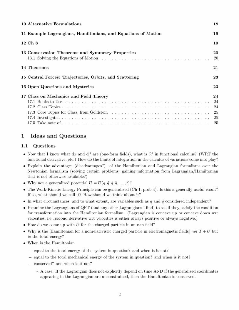
• Now that I know what dx and df are (one-form fields), what is δf in functional calculus? (WRT thefunctional derivative, etc.) How do the limits of integration in the calculus of variations come into play?• Explain the advantages (disadvantages?) of the Hamiltonian and Lagrangian formalisms over the

Newtonian formalism (solving certain problems, gaining information from Lagrangian/Hamiltonianthat is not otherwise available?)• Why not a generalized potential U = U(q, q, q, ...q, . . . , t)?• The Work-Kinetic Energy Principle can be generalized (Ch 1, prob 4). Is this a generally useful result?

If so, what should we call it? How should we think about it?• In what circumstances, and to what extent, are variables such as q and q considered independent?• Examine the Lagrangians of QFT (and any other Lagrangians I find) to see if they satisfy the condition

for transformation into the Hamiltonian formalism. (Lagrangian is concave up or concave down wrtvelocities, i.e., second derivative wrt velocities is either always positive or always negative.)• How do we come up with U for the charged particle in an e-m field?• Why is the [Hamiltonian for a nonrelativistic charged particle in electromagnetic fields] not T +U but

is the total energy?• When is the Hamiltonian

− equal to the total energy of the system in question? and when is it not?− equal to the total mechanical energy of the system in question? and when is it not?− conserved? and when is it not?

∗ A case: If the Lagrangian does not explicitly depend on time AND if the generalized coordinatesappearing in the Lagrangian are unconstrained, then the Hamiltonian is conserved.

2

If you include the constrained angular coordinate in the Lagrangian as a generalized coordinate,then the theorem is no longer true. You have to use Lagrange multipliers or some other techniqueto deal with the constrained system i.e. to find equations of motion.http://www.physicsforums.com/archive/index.php/t-87978.html

• Are scientists trying to come up with “the most fundamental Hamiltonian” (of the universe), andshould it be conserved? (Perhaps once they come up with this fundamental, conserved Hamiltonian,then they’ll know how to break it up and to examine subsystems (of the universe), which may havenonconserved Hamiltonians.)• What is the difference between a dissipation function and a generalized potential?• Is D’Alembert’s principle equivalent to Newton’s second law, as Wikipedia claims. (Article: D’Alembert’s

principle)

1.2 Things to Look Into

From Goldstein’s [1] index:• (Principle of) Virtual work• Virial of Claussius• Symplectic notation, for Hamilton’s equations

Show principle of maximal aging implies principle of least action. (http://www.eftaylor.com/index.html)

1.3 Unit Questions

Are they really the same? If not, how are they different?• torque (τ = r× F) has the “same” units as energy (W =

∫F · ds): m×N “=” N ·m

• angular momentum (L = r× p) has the “same” units as action (S =∫Ldt): m× kg · m

s “=” J · s• volumetric flux density (... meters cubed of substance per second per meter squared of surface through

which the substance passes) has the “same” units as velocity (meters traversed per second): m3

s /m2

“=” m/s

2 The Big Picture

Classical mechanics includes the general theory of relativity and what else? (See notes on relativity fordetails of relativistic mechanics.)

2.1 Historical Development

D’Alembert’s principle? Hamilton-Jacobi eqns?• 1772-88 - The French and Italian mathematician and astronomer Joseph-Louis Lagrange (1736-1813)

reformulates Newtonian mechanics into Lagrangian mechanics.• - French mathematician Adrien-Marie Legendre (1752-1833)• - German mathematician Carl Gustav Jacob Jacobi (1804-1851)• 1833 - The Irish mathematician William Rowan Hamilton (1805-1865) invents a reformulation of clas-

sical mechanics – Hamiltonian mechanics.• 1834 - Hamilton’s principle

3

• 1867 - The terms generalized coordinates, generalized velocities, and generalized momenta were intro-duced by Sir William Thomson (later, Lord Kelvin) and P. G. Tait in their famous treatise NaturalPhilosophy.• 1870 - Rudolf Julius Emanuel Clausius (1822-1888) proves the scalar virial theorem.

3 Notation

• A set of generalized coordinates {q1, q2, q3, . . . , qn} may be denoted {qj}j∈Nn , or qj , or q, or simply q.This last notation will be most common, and it should be clear from the context whether q representsone coordinate or a set of coordinates. (If unsure, assume q represents a set of coordinates rather thanone coordinate.)

− The same goes for canonical momenta: {p1, p2, p3, . . . , pn} may be denoted {pj}j∈Nn , or pj , or p, orsimply p.

• There is an ambiguity between the polar-angle component of Cartesian momentum and the canonicalmomentum conjugate to the polar angle, both of which may be denoted pθ. (Similar ambiguities arisefor other momenta.)

− How shall I resolve this ambiguity? Use pθ or θp?

• Dot notation (Newton’s fluxion)

q ≡ dqdt

(I’m not sure, but this might also sometimes be used to denote the partial time derivative.)What about when we go from a particle Lagrangian to a field Lagrangian density:

∂L

∂q→ ∂L

∂(∂tφ)?

ϕ ≡ ∂tϕ ?

• Total derivativedt ≡

ddt

Change over time given an arbitrary change in all other variables, if any.• Partial derivative

∂t ≡∂

∂t

Change over time given that all other variables, if any, are constant.

4 Mathematics

• Standard Calculus• Functional Calculus• Differential Geometry• (Lie Groups, Algebras, Representations?)• Small Theorems

− Euler’s thm - If f(yk) is a homogeneous function of the yk that is of degree n, then∑

k yk∂f∂yk

= nf .

4

5 Terms and Quantities

• Position

• Time

• Velocity, Acceleration, Jerk, etc.

• Inertia

• Momentum

• Force

• Mass

• Moments (of force, of mass, of inertia, etc)

• System

• Degrees of Freedom

• Coordinates

• Generalized Coordinates

• Equation of Motion

• Constraint

• Equation of Constraint

• Holonomic Constraints and Systems

• Monogenic Forces and Systems

• T (v), T (q) Kinetic EnergyThe energy of motion of objects relative to each other.

• V (r), V (q) Potential Energy (Conservative Potential)

• U(q, q, t) Generalized Potential(also U(q, q) “Velocity-dependent Potential”)

• F Dissipation Function(also Rayleigh’s dissipation function, or viscous dissipation function)

• Stress Tensor - Energy-Momentum-Stress TensorTµν is “the flux of 4-momentum pµ across a surface of constant xν .”Or Tµν is “the flux of 4-momentum component pµ across a surface of constant xν .”T 00, the “flux of p0 (energy) in the x0 (time) direction”, is the rest-frame energy densityMechanical Stress Tensor - stress, strain, compression, pressure, viscosity (normal and tangentialtractions, or equivalently, direct and shear stresses)See http://www.bun.kyoto-u.ac.jp/~suchii/extrem.aging.htmlStress Holor T ij as a sub-holor of Tµν

Dust and perfect fluid (which can be completely specified by two quantities, the rest-frame energydensity ρ and an isotropic rest-frame pressure p)

5

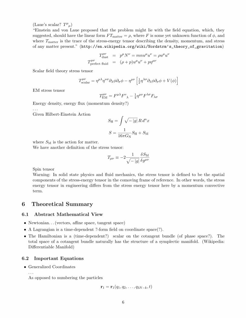
(Laue’s scalar? T µµ )

“Einstein and von Laue proposed that the problem might lie with the field equation, which, theysuggested, should have the linear form FTmatter = ρ, where F is some yet unknown function of φ, andwhere Tmatter is the trace of the stress-energy tensor describing the density, momentum, and stressof any matter present.” (http://en.wikipedia.org/wiki/Nordstrm’s_theory_of_gravitation)

Tµνdust = pµNν = mnuµuν = ρuµuν

Tµνperfect fluid = (ρ+ p)uµuν + pηµν

Scalar field theory stress tensor

Tµνscalar = ηµληνσ∂λφ∂σφ− ηµν[

12η

λσ∂λφ∂σφ+ V (φ)]

EM stress tensorTµνEM = FµλF νλ − 1

4ηµνF λσFλσ

Energy density, energy flux (momentum density?). . .Given Hilbert-Einstein Action

SH =∫ √

− |g|Rdnx

S =1

16πGNSH + SM

where SM is the action for matter.We have another definition of the stress tensor:

Tµν ≡ −21√− |g|

δSM

δgµν

Spin tensorWarning: In solid state physics and fluid mechanics, the stress tensor is defined to be the spatialcomponents of the stress-energy tensor in the comoving frame of reference. In other words, the stressenergy tensor in engineering differs from the stress energy tensor here by a momentum convectiveterm.

6 Theoretical Summary

6.1 Abstract Mathematical View

• Newtonian. . . (vectors, affine space, tangent space)• A Lagrangian is a time-dependent ?-form field on coordinate space(?).• The Hamiltonian is a (time-dependent?) scalar on the cotangent bundle (of phase space?). The

total space of a cotangent bundle naturally has the structure of a symplectic manifold. (Wikipedia:Differentiable Manifold)

6.2 Important Equations

• Generalized Coordinates. . .As opposed to numbering the particles

r1 = r1(q1, q2, . . . , q3N−k, t)

6

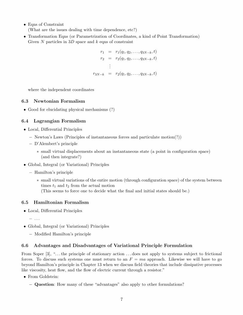
• Eqns of Constraint(What are the issues dealing with time dependence, etc?)• Transformation Eqns (or Parametrization of Coordinates, a kind of Point Transformation)

Given N particles in 3D space and k eqns of constraint

r1 = r1(q1, q2, . . . , q3N−k, t)r2 = r2(q1, q2, . . . , q3N−k, t)

...r3N−k = r2(q1, q2, . . . , q3N−k, t)

where the independent coordinates

6.3 Newtonian Formalism

• Good for elucidating physical mechanisms (?)

6.4 Lagrangian Formalism

• Local, Differential Principles

− Newton’s Laws (Principles of instantaneous forces and particulate motion(?))− D’Alembert’s principle

∗ small virtual displacements about an instantaneous state (a point in configuration space)(and then integrate?)

• Global, Integral (or Variational) Principles

− Hamilton’s principle

∗ small virtual variations of the entire motion (through configuration space) of the system betweentimes t1 and t2 from the actual motion(This seems to force one to decide what the final and initial states should be.)

6.5 Hamiltonian Formalism

• Local, Differential Principles

− . . .

• Global, Integral (or Variational) Principles

− Modified Hamilton’s principle

6.6 Advantages and Disadvantages of Variational Principle Formulation

From Soper [3], “. . . the principle of stationary action . . . does not apply to systems subject to frictionalforces. To discuss such systems one must return to an F = ma approach. Likewise we will have to gobeyond Hamilton’s principle in Chapter 13 when we discuss field theories that include dissipative processeslike viscosity, heat flow, and the flow of electric current through a resistor.”• From Goldstein:

− Question: How many of these “advantages” also apply to other formulations?

7

− Coordinate Invariance: Formulation refers to kinetic and potential energies, which are alwaysdefinable and independent of coordinate system.

− Universality of technique: Lagrangian formulation can be extended easily to describe systemsthat are not normally considered in dynamics, such as elastic fields, the electromagnetic field, andfield properties of elementary particles.

− Formal similarity of phenomena: Formal similarities between different kinds of systems (such aselectrical circuits and mechanical systems) become apparent. (Terms normally reserved for electricalcircuits, such as reactance and susceptance, are the accepted modes of expression in much of thetheory of vibrations of mechanical systems.1)

− Structural analogy of fields of study: Lagrange’s and Hamilton’s principles together forma copact invariant way of implying the mechanical equations of motion. This works outside ofmechanics also: variational principles can be used to express the “equations of motion,” whether theybe Newton’s equations, Maxwell’s equations, or the Schrodinger equation. So, when a variationalprinciple is used as the basis of formulation of all fields, they will exhibit, at least to some degree,a structural analogy.

− The methods of quantization were first developed for particle mechanics, starting essentiallyfrom the Lagrangian formulation of classical mechanics. By describing the electromagnetic fieldby a Lagrangian and corresponding Hamilton’s variational principle, it is possible to carry overthe methods of particle quantization to construct a quantum electrodynamics.

• From Marion and Thorton:

− The Newtonian approach emphasizes an outside agency acting on a body (the force), while theLagrangian method deals only with quantities associated with the body (the kinetic and potentialenergies). In certain situations it may not be possible to state explicitly all the forces acting ona body, as is sometimes the case for forces of constraint and as is normally the case for quantummechanical systems where we normally know the eneries but not the forces.

6.7 Other Stuff

From Abers, page 47, we have that the classical equation of motion is

A(t) = {A,H}+ ∂t

7 Newtonian Mechanics

7.1 Forces, Newton’s Laws, and Conservation

• Newton’s Laws of Motion

− N1: Interia

∗ Statement of kinematics in absence of forces (interaction). Special case of N2.∗ ⇒ CLM and CAM for elementary particles with no external forces. (Not observed, not inter-

acting.)

− N2: Force (Action) and Momentum

∗ How does one define a force and mass?1For a detailed exposition, see H. F. Olson, Solutions of Engineering Problems by Dynamic Analogues (New York: Van

Nostrand 1966).

8

− N3: Coaction

∗ WN3∗ SN3

• N2: Various forms of Newton’s Second Law (N2) depend on the Laws of Coaction (forms of Newton’sThird Law, N3)

− Forms that are always valid: Single particle, Superposition of multiple particles (both “linear” andangular forms, correct?)

• WN3: Weak Law of Coaction

− WN3: The forces that two particles exert on each other are equal and opposite.− ⇒ N2 for Systems of particles is valid (Using total mass, center of mass, net force)− In absense of external forces

Conservation of total linear momentum assumes WN3 to be true(so the internal forces cancel)

• SN3: Strong Law of Coaction

− SN3: The forces that two particles exert on each other are equal and opposite and directed alongthe line joining the particles.

− ⇒ N2 for Angular momenta and forces (torque) is valid− In absense of external forces

Conservation of total angular momentum assumes SN3 to be true(so the internal forces are central and cancel)

• N3 (in either form) DOES NOT hold for all forces (in the Newtonian picture) (. . . if you includeeverything such as momentum of fields, etc, then, in some sense, N3 always holds). (elaborate onthis. . . )• PLN2 ⇔ PAN2 ⇔ CPLM ⇔ CPAM

PLN2 + WN3 ⇔ SLN2 ⇔ CTLMPAN2 + SN3 ⇔ SAN2 ⇔ CTAMC = conservation of, P = particulate, T = total, S = systemic/strong, W = weak, L = linear, A =angular, M = momentum, N = Newton’s, 2 = second law, 3 = third law• Mechanical Energy:

Note that in some circumstances, a force may be given by the gradient of a scalar function F = −∇Vand the mechanical energy E = T + V may still be defined, but

− W 6= ∆V− E is NOT conserved

7.1.1 Examples

• F = −∇V where V = V (|r2 − r1|) = V (R)⇒ SN3• F = −∇V where V = V (|r2 − r1| , |v2 − v1| , |s2 − s1|)⇒ WN3 only

7.2 Extraneous Material

• Center of mass 6= Center of gravity•

9

8 Lagrangian Formalism

The Lagrangian formulation of classical mechanics• (in its usual holonomic form) eliminates the constraining forces from the equations of motion• utilizes scalar functions (L, T , U), which can simplify problems

(Describe how, why)

8.1 Fundamentals

Constraints Geometric limits on the system where the forces enforcing theselimits are not necessarily known (apriori or something like that)(always geometric?)

Generalized Coordinates Coordinates of any type that fully distinguish a state of the system,consistent with the constraints

Virtual Displacement and δr, δqVirtual Work F δr, Qδq

Variation and δr(t), δq(t)First Variation δF (q, t) = ∂F

∂q δq + ∂2F∂q2

(δq)2 + · · · = ∂F∂q δq

Functional DifferentiationandFunctional Integration

Principle of Virtual Work Virtual-work-less constraining forces∑

i Fci · δr = 0,

with equilibrium F = 0

⇒∑

i Foi · δr = 0

(IS this a sum over particles? If not, then the transformation togeneral coordinates may need an integral?)

• holonomic constraints, systems• nonholonomic constraints, systems

8.2 Local, Differential Formulation: D’Alembert’s Principle and Lagrange’s Equa-tions

The physical (and local) concept of virtual-work-less constraint, together with Newton’s second law of mo-tion, generates all of the equations of the Lagrangian and Hamiltonian formulations of classical mechanics.It is required in both the holonomic and nonholonomic equations.

“In practice, the restriction (to virtual-work-less constraints) presents little handicap to the applications,as most problems in which the nonholonomic formalism is used relate to rolling without slipping, wherethe constraints are obviously workless.”

I give some names to the intermediate equations for organizational and mental-recall purposes, and Iput a star (?) by the equations that seem to be most fundamental or important to remember:

10

D’Alembert’s Principle Virtual-work-less constraining forces∑

i Fci · δr = 0 and N2 F− p = 0

⇒∑

i

(Foi − pi

)· δr = 0 ?

with generalized coordinate and force transformations:

⇒∑

j

[Qoj −

{ddt

(∂T∂qj

)− ∂T

∂qj

}]δqj = 0 ?

“D’Alembert’s Principle D’Alembert’s Principle, with a potential:with Gnzd. Potential” some applied forces derivable from a generalized potential U(qj , qj , t)

⇒∑

j

[Qrj −

{ddt

(∂L∂qj

)− ∂L

∂qj

}]δqj = 0

“Monogenic D’Alembert’s Principle, with monogenic forces:D’Alembert’s Principle” all applied forces derivable from a generalized potential U(qj , qj , t)

⇒∑

j

[ddt

(∂L∂qj

)− ∂L

∂qj

]δqj = 0

“Holonomic D’Alembert’s Principle, with holonomic constraints:D’Alembert’s Principle” (⇒ independent qj ’s)

⇒ ddt

(∂T∂qj

)− ∂T

∂qj= Qo

j

“Generalized D’Alembert’s Principle, with holonomic constraints and a potential:Lagrange’s Eqn” some applied forces derivable from a generalized potential U(qj , qj , t)

⇒ ddt

(∂L∂qj

)− ∂L

∂qj= Qr

j ?

“Monogenic Generalized D’Alembert’s Principle, with holonomic constraints and monogenic forces:Lagrange’s Eqn” all applied forces derivable from a generalized potential U(qj , qj , t)

⇒ ddt

(∂L∂qj

)− ∂L

∂qj= 0 ?

Lagrange’s Eqn D’Alembert’s Principle, with holonomic constraintsand monogenic conservative forces:all applied forces derivable from a conservative potential U(qj)

⇒ ddt

(∂L∂qj

)− ∂L

∂qj= 0

“Dissipative Generalized Generalized Lagrange’s Equation, with nonconservative forcesLagrange’s Eqn” derivable from a dissipation function F d

i = −∂F∂vi

, so Qdj = −∂F

∂ qj

⇒ ddt

(∂L∂qj

)− ∂L

∂qj+ ∂F

∂ qj= Qn

j ?

Nonholonomic Monogenic D’Alembert’s Principle,Lagrange’s Eqn with special nonholonomic eqns of constraint

∑j akjdqj + aktdt = 0

and usage of the method of Lagrange (undetermined) multipliers:

⇒ ddt

(∂L∂qj

)− ∂L

∂qj=∑

k λkakj (= Qcj) j ∈ Nn ?

and∑

j akj qj + akt = 0 k ∈ Nm ?

The “Dissipative Generalized Lagrange’s Equation” is the most generalized, concept-packed holonomicequation, so it should definitely be memorized. The Nonholonomic Lagrange’s Equation is used lessfrequently but should be kept in mind.

11

• F = Fc + Fo

Fo = Fp + Fr

Fr = Fd + Fn

“c” for constraint, “o” for other, “p” for derivable from a generalized potential, “r” for remaining, “d”for derivable from a dissipation function, “n” for not derivable (are there any such things, or mightthey be derivable from something else?)• Q = Qc +Qo = Qc +Qp +Qr = Qc +Qp +Qd +Qn

(The usual holonomic Lagrangian formalism gets rid of the constraining forces.)• Kinetic energy T

T =∑i

12miv

2i =

∑i

12mi

(∑j

∂ri∂qj

qj + ∂ri∂t

)2

= M0 +∑j

Mj qj + 12

∑jk

Mjkqj qk

= T0 + T1 + T2

• Generalized force Qj (conjugate? to the generalized coordinate qj)

? Qj ≡∑i

Fi ·∂ri∂qj

Qoj ≡

∑i

Foi ·∂ri∂qj

Qpj = d

dt

(∂U∂qj

)− ∂U

∂qj

How does one come up with such a potential?

Qdj =

∑i

Fdi ·∂ri∂qj

=∑i

−∂F

∂vi· ∂ri∂qj

=∑i

−∂F

∂vi· ∂vi∂qj

= −∂F

∂qj

• Lagrangian LL(q(t), q(t), t) ≡ T (q(t))− U(q(t), q(t), t)

The dependence of L on time may arise if the constraints are time-dependent, if the transformationequations connecting the rectangular and generalized coordinates explicitly contain the time, or if thegeneralized potential is explicitly time-dependent.

8.2.1 Freedom of Lagrangian

(Gauge?) freedom of the Lagrangian:

L′(q, q, t) = L(q, q, t) +dFdt

While L = T −V is always a suitable way to construct a Lagrangian for a conservative system, it DOESNOT provide the only Lagrangian suitable for the given system; you may also use L′ = T − V + dtF .

12

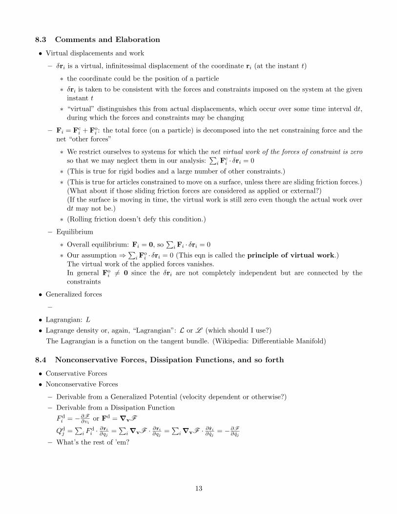
8.3 Comments and Elaboration

• Virtual displacements and work

− δri is a virtual, infinitessimal displacement of the coordinate ri (at the instant t)

∗ the coordinate could be the position of a particle∗ δri is taken to be consistent with the forces and constraints imposed on the system at the given

instant t∗ “virtual” distinguishes this from actual displacements, which occur over some time interval dt,

during which the forces and constraints may be changing

− Fi = Fci + Fo

i : the total force (on a particle) is decomposed into the net constraining force and thenet “other forces”

∗ We restrict ourselves to systems for which the net virtual work of the forces of constraint is zeroso that we may neglect them in our analysis:

∑i F

ci · δri = 0

∗ (This is true for rigid bodies and a large number of other constraints.)∗ (This is true for articles constrained to move on a surface, unless there are sliding friction forces.)

(What about if those sliding friction forces are considered as applied or external?)(If the surface is moving in time, the virtual work is still zero even though the actual work overdt may not be.)∗ (Rolling friction doesn’t defy this condition.)

− Equilibrium

∗ Overall equilibrium: Fi = 0, so∑

i Fi · δri = 0∗ Our assumption ⇒

∑i F

oi · δri = 0 (This eqn is called the principle of virtual work.)

The virtual work of the applied forces vanishes.In general Fo

i 6= 0 since the δri are not completely independent but are connected by theconstraints

• Generalized forces

−

• Lagrangian: L• Lagrange density or, again, “Lagrangian”: L or L (which should I use?)

The Lagrangian is a function on the tangent bundle. (Wikipedia: Differentiable Manifold)

8.4 Nonconservative Forces, Dissipation Functions, and so forth

• Conservative Forces• Nonconservative Forces

− Derivable from a Generalized Potential (velocity dependent or otherwise?)− Derivable from a Dissipation FunctionF di = −∂F

∂vior Fd = ∇vF

Qdj =

∑i F

di ·

∂ri∂qj

=∑

i ∇vF · ∂ri∂qj=∑

i ∇vF · ∂ ri∂ qj= −∂F

∂ qj

− What’s the rest of ’em?

13

8.5 Method of Lagrange Multipliers

• Usable whenever the eqns of constraint are in the form∑j

alj dqj + alt dt = 0

and we may take, since virtual displacements dqj = δqj imply that dt = 0,∑k

alj δqj = 0 (⇒ virtual-work-less constraints)

• Includes holonomic constraints. Useful when

(1) it’s convenient to reduce all the q’s to ind coords(2) want to solve for the forces of constraint

We get n+m equations for n+m unknowns: (the first being Lagrange’s Eqns for nonholonomic systems)

ddt

(∂L

∂qj

)− ∂L

∂qj=∑k

λkakj (= Qc +Qo ? ) j ∈ Nn

∑j

akj qj + akt = 0 k ∈ Nm

8.6 Global, Integral Formulation: Hamilton’s Principle and the Euler-Lagrange Equa-tions

8.6.1 Assumptions

• Monogenic systems• (Virtual-work-less systems?)

Hamilton’s Principle δI ≡ δ∫ t2t1

dt L = 0The motion of the system from time t1 to t2 is such that the lineintegral I =

∫ t2t1

dt L, where L = T − V , has a stationary value forthe correct path of the motion.I.e., the motion is such that the variation of the line integral I forfixed t1 and t2 is zero:

δI = δ∫ t2t1

dt L(q1, . . . , qn; q1, . . . , qn; t) = 0(Can extend this to include some nonholonomic systems, but thisformulation is most useful for holonomic systems, wherein a La-grangian of independent coordinates can be set up.)

Euler-Lagrange Eqns ∂f∂yi− d

dx∂f∂yi

= 0

yi ≡ dyidx ; i ∈ {1, 2, . . . , n}

x→ t, yi → qi, f(yi, yi, x)→ L(qi, qi, t)Extensions: Consider f = f(yi, yi, yi,

...yi, . . . , x), or use several pa-

rameters xj , yielding a multiple integral and derivatives of each yiwith respect to each xj , and/or consider variations in which theend points are not held fixed.

14

• (see Goldstein pg 48: “In this dress, Hamilton’s principle says... δ∫ t2t1

dt T = −∫ t2t1

∑kQkδqk dt)

• “The variational principle formulation has been justly described as ‘elegant,’ for in the compact Hamil-ton’s principle is contained all of the mechanics of holonomic systems with forces derivable from poten-tials. The principle has the further merit that it involves only physical quantities that can be definedwithout reference to a particular set of generalized coordinates, namely, the kinetic and potential ener-gies.”• Lagrange’s eqns ⇔ Hamilton’s principle• (Hamilton’s principle⇒ Lagrange’s eqns) is more important than the converse (why? since Hamilton’s

principle yields more? Like what?)

15

9 Hamiltonian Formalism

9.1 Legendre Transformations, Variational Principles, and Hamilton’s Equations

Original Function Legendre Transform

y(x) ψ(p)

A collection of points in the xy-plane As a description of the original function:a collection of tangent lines of slope p andy-intercept ψ

As a description of the Legendre trans-form: a collection of tangent lines of slope−x and ψ-intercept y

A collection of points in the pψ-plane

• Original Function

− Domain: Rn

− Codomain: R (for convenience, imagine each value as a different color)

• Original Function Level Subspaces (generalization of level curves)

− 1D domain: 1-2 points (one color)− 2D domain: monochromatic curves− 3D domain: monochromatic surfaces

• Tangent Objects

− 1D domain: line (hyperpoint of constant color-velocity)− 2D domain: cone/pyramid (hyper-(closed curve) with continuous distribution of color-velocity that

is constant in time)possibly also hyper-(curve segment)

− 3D domain: hyperbubble (hyper-(closed surface))possibly also hyper-(bubble segment)

• Osculating Subspace for Orignal Function and Tangent Object

− 1D domain: 1 point (one color)− 2D domain: polychromatic curves− 3D domain: polychromatic surfaces

•

16

Energy function h h(q, q, t) =∑

j qj∂L∂qj− L(q, q, t)

• The energy function h is identical in value with the Hamiltonian H but is a function of n + 1independent variables (the q’s plus t) and the q’s (which depend on the q’s) while H is a functionof 2n+ 1 independent variables.• h is not necessarily the mechanical energy, and it is not necessarily conserved.• Whereas the Lagrangian is uniquely fixed for each system by the prescription L = T − U , in-

dependent of the choice of generalized coordinates, the energy function h depends in magnitudeand functional form on the specific set of generalized coordinates. For one and the same system,various energy functions h of different physical content can be generated depending on how thegeneralized coordinates are chosen.• If frictional forces are present and derivable from a dissipation function F , then F is related to

the decay of h.

Initial Definition of Canonical Momentum pi = ∂L∂qi

Also called constitutive relations.

from Lagrange’s (monogenic, nonrel.) Equation pi = ∂L∂qi

Initial Definition of the Hamiltonian H(q, p, t) = qi pi − L(q, q, t)with summation over i and q = q(q, p, t)

Modified Hamilton’s Principle δI =∫ t2t1

dt(qipi −H(q, p, t)

)= 0

Hamilton’s (Canonical) Equations qi = ∂H∂pi

−pi = ∂H∂qi

? −∂L∂t = ∂H

∂t

Hamilton’s Equations in Matrix/Symplectic Notation η = J ∂H∂η

• η is the canonical variable vector:ηi = qi, ηn+i = pi; i ≤ n

• J =

(0 I−I 0

), where 0 and I are n× n

− (Properties of the matrix J here)−

•(∂H∂η

)i≡ ∂H

∂ηi

About the symplectic notation: “Considerable ingenuity has been exercised in devising nomenclatureschemes that result in entirely symmetric equations, or combine the two sets into one. Most of these schemeshave only oddity value, but one (the symplectic notation) has proved to be an elegant and powerful toolfor manipulating the canonical equations and allied expressions.”

9.2 Constructing the Hamiltonian via the Lagrangian Formulation

1. With a chosen set of generalized coordinates, qi, the Lagrangian L(qi, qi, t) is constructed.

2. The conjugate momenta are defined as functions of qi, qi, and t by the (initial) definition of pi =∂L/∂qi.

17

3. The Hamiltonian is formed using H(q, p, t) = qi pi − L(q, q, t). At this stage one has h instead of H,or rather some mixed function of qi, qi, pi, and t.

4. The equations pi = ∂L/∂qi are then inverted to obtain qi as functions of (q, p, t). Possible difficultiesin the inversion SHOULD BE ADDRESSED SOMEWHERE.

5. The results of the previous step are then applied to eliminate q from H so as to express it solely asa function of (q, p, t)

9.3 Variational Principles

• action, abbreviated action, (Maupertuis action)• Variational Principles of Mechanics

“A host of similar variational principles for classical mechanics can be derived in bewildering variety.The variational principles in themselves contain no new physical content (with respect to Newton’sLaws or Lagrange’s equations), and they rarely simplify the practical solution of a given mechanicalproblem. Their value lies chiefly as starting points for new formulations of the theoretical structure ofclassical mechanics. For this purpose Hamilton’s principle is especially fruitful, and to a lesser extent,so also is the principle of least action. The others have proved to be of little use, except as they haveled to fruitless teleological speculations (on final cause or purpose and design).”

− Principle of Stationary Action (“Least Action”)− Jacobi’s for of the least action principle− Hertz’s principle of least curvature− Fermat’s principle in geometrical optics (of least time for light)− (Principle of maximal proper time in general relativity)

9.4 Canonical Transformations

• Passive• Active

10 Alternative Formulations

• Routhian∼ “. . . Routh’s is most useful in engineering applications. But the Routhian is a sterile hybrid of theLagrangian and Hamiltonian pictures; for developing various formalisms of classical mechanics, thecomplete Hamiltonian formulation is more fruitful.”• Various others

18

11 Example Lagrangians, Hamiltonians, and Equations of Motion

Nonrelativistic charged particle in electromagnetic fields (mass m, charge q)

U = q(Φ−A ·v) U(r, r, t) = q(Φ(r, t)−A(r, t) · r

)L = 1

2mv2 − qΦ + qA ·v L(r, r, t) = 12mr2 − qΦ(r, t) + qA(r, t) · r

H = 12m(p− qA)2 + qΦ H(r,p, t) = 1

2m(p− qA(r, t))2 + qΦ(r, t)

• The Hamiltonian is not T + U , but it is the total energy (WHY?)

Some other situation

When a Hamiltonian Equals Total Energy

• The Lagrangian is the sum of functions each homogeneous in the generalized velocitiesof degree 0, 1, and 2, respectively. So H = L2 − L0 (cf. Eq. 2-57 in Goldstein).• The equations defining the generalized coordinates don’t depend on time explicitly, soL2 = T .• The forces are derivable from a conservative potential V , so L0 = −V and T +V = E.

H = T + V = E

Hamiltonian when Lagrangian has Simple Form

• L = L0 + L1 + L2

L(q, q, t) = L0(q, t) + kTq +12qTT q

− T is a symmetric matrix (and what about the positive definite property of thekinetic energy? see below)

• p = T q + k

− q = T−1(p− k)− T−1 normally exists by virtue of the positive definite property of the kinetic energy

• h = 12 qTT q− L0

H(q, p, t) =12

(p− k)TT−1(p− k)− L0(q, t)

Something else

12 Ch 8

• Legendre Transformations and the Hamilton Equations of MotionWhen coming up with the Hamiltonian formulation, we say

pj ≡∂L(qi, qi, t)

∂qj

19

but when using the Hamiltonian formulation we assume pj is independent of qj . Can we recoverthis equation? If so, is it different in this situation because it’s an equation of motion rather than adefinition?• Ignorable Coordinates and Conservation Theorems• Routh’s Procedure and Oscillations about Steady Motion• The Hamiltonian Formulation of Relativistic Mechanics• Derivation of Hamilton’s Equations from a Variational Principle• The Principle of Least Action

13 Conservation Theorems and Symmetry Properties

13.1 Solving the Equations of Motion

• A sustem of n degrees of freedom will have n differential eqns that are second order in time.• The solution of each eqn will require two integrations reulting in 2n constants of integration.

− Could be the intial conditions (the n qj ’s and the n qj ’s at the initial time ti.)

• Canonical or Conjugate Momentum (generalized momentum conjugate to the generalized coordinateqj)

pj ≡∂L

∂qj

If qj is not Cartesian, then pj will not necessarily have the dimensions of a linear momentum. When qjis Cartesian, if the potential is velocity-dependent, then the generalized momentum will not be identicalwith the ususal mechanical momentum.• If a coordinate is ignorable (the Lagrangian is independent of that coordinate), then its conjugate

momentum is conserved, or contant. This is more general than the Newtonian momentum conservationlaws (which require WN3 or SN3). E.g., for a charged particle in an electromagnetic field,

px = mx+ qAx

is conserved if Φ and A are independent of x. (qAx is the electromagnetic linear momentum associatedwith the field of the particle)• energy function

h(q, q, t) =∑j

qj∂L

∂qj− L

dhdt

= −∂L∂t

• Euler’s theorem, . . . , h = T + V in some cases but not others, conserved in some cases but not others,. . . , dissipation function

dhdt

= −2F − ∂L

∂t

sometimes:dEdt

= −2F

20

14 Theorems

• Liouville’s Theorem and Equation (of classical statistical and Hamiltonian mechanics)The Liouville equation describes the time evolution of phase space measure (a.k.a. distributionfunction in physics).

dtρ = ∂tρ+d∑i=1

(∂ρ∂qi

qi + ∂ρ∂pi

pi

)= 0

∂tρ = −{ρ,H}

(∂t + L)ρ = 0

where

L ≡d∑i=1

(∂H∂pi

∂∂qi− ∂H

∂qi∂∂pi

)is the Liouvillian or Liouville operator.

− Related to symplectic topology, ergodic theory, Hamiltonian flow, conservation (Noether’s Thm)etc.

− The equation is valid for both equilibrium and nonequilibrium systems. It is a fundamentalequation of nonequilibrium statistical mechanics. Generalized to collisional systems it is calledthe Boltzmann equation.

− The equation is integral to the proof of the fluctuation theorem from which the second law ofthermodynamics can be derived. It is also the key component of the derivation of Green-Kuborelations for linear transport coefficients such as shear viscosity, thermal conductivity or electricalconductivity.

− Virtually any textbook on Hamiltonian mechanics, advanced statistical mechanics, or symplecticgeometry will derive the Liouville theorem.

− Quantum analogues: Lindblad equation for the density matrix ρ, Ehrenfest theorem (each missingthe last piece?)

∂tρ = − 1i~

[ρ,H]dt ρ = − 1i~

[ρ,H]− 1~∑n,m

hn,m (ρLmLn + LmLnρ− 2LnρLm) + h.c.

dt 〈A〉 =

1i~⟨[A,H]

⟩ (+ 〈∂tA〉

)from (http://en.wikipedia.org/wiki/Liouville’s_theorem_(Hamiltonian)). . . why are thelast pieces not included?The sign difference follows from the assumption that the operator is stationary and the state istime-dependent.

• Helmholtz Theorem (of classical mechanics)This theorem should be distinguished from Helmholtz’s theorem in vector calculus (the fundamentaltheorem of vector calculus, relating to Helmholtz decomposition) and Helmholtz’s theorems in fluidmechanics, all named after Hermann von Helmholtz.

• Generalized Helmholtz Theorem

21

• (1873) Bertrand’s Theorem of central force, two-body motionThe only central forces that result in closed orbits for all bound particles are the inverse square lawand Hooke’s law.

• General characteristics ⇒ quantitative information

− The degenerate character of orbits in a gravitational field fixes the form of the force law.Degenerate means that the periods of oscillation of the body in two variables (r and θ) arecommensurate, so that the orbit is closed.(It is not necessary to use the elliptic character of the orbits to arrive at the gravitational forcelaw.)(“Later on we shall encounter other formulations of the relation between degeneracy and thenature of the potential.”)

• Larmor’s TheoremTo first order in B, the effect of a constant magnetic field on a classical system is to superimpose on itsnormal motion a uniform precession with angular frequency ωl = −qB/2m (the Larmor frequency).

• Noether’s TheoremHas a Lagrangian formulation and a Hamiltonian formulation.

Relates symmetries and conservation laws.

(Is this what I start with? [See Peskin & Schroeder pg 17] Given that the action is invariant undera transformation φ′ = eiajgjφ, or, equivalently, given that the Lagrangian density is invariant up toa four-divergence under the transformation, we have)(

L′(x) = L(x) + δL(x))(

where δL(x) = δαj ∂µJ µj (x))

S =∫

d4x L(φα, ∂µφα

)0 = δS

=∫

d4x[∂L∂φα

δφα + ∂L∂(∂µφα) δ

(∂µφα

)]

=∫

d4x

���

�����

����:0{

∂L∂φα− ∂µ

(∂L

∂(∂µφα)

)}δφα + ∂µ

{∂L

∂(∂µφα) δφα

}⇒ ∂µ

{∂L

∂(∂µφα) δφα

}≡ ∂µjµ = 0

δφα = i δaj (gj)αβ φβφ′ = eiajgjφ

jµ ≡ ∂L∂(∂µφα) δφα

= ∂L∂(∂µφα)

(i δaj (gj)αβ φβ

)= i ∂L

∂(∂µφα) δaj (gj)αβ φβ∂µj

µ = 0

22

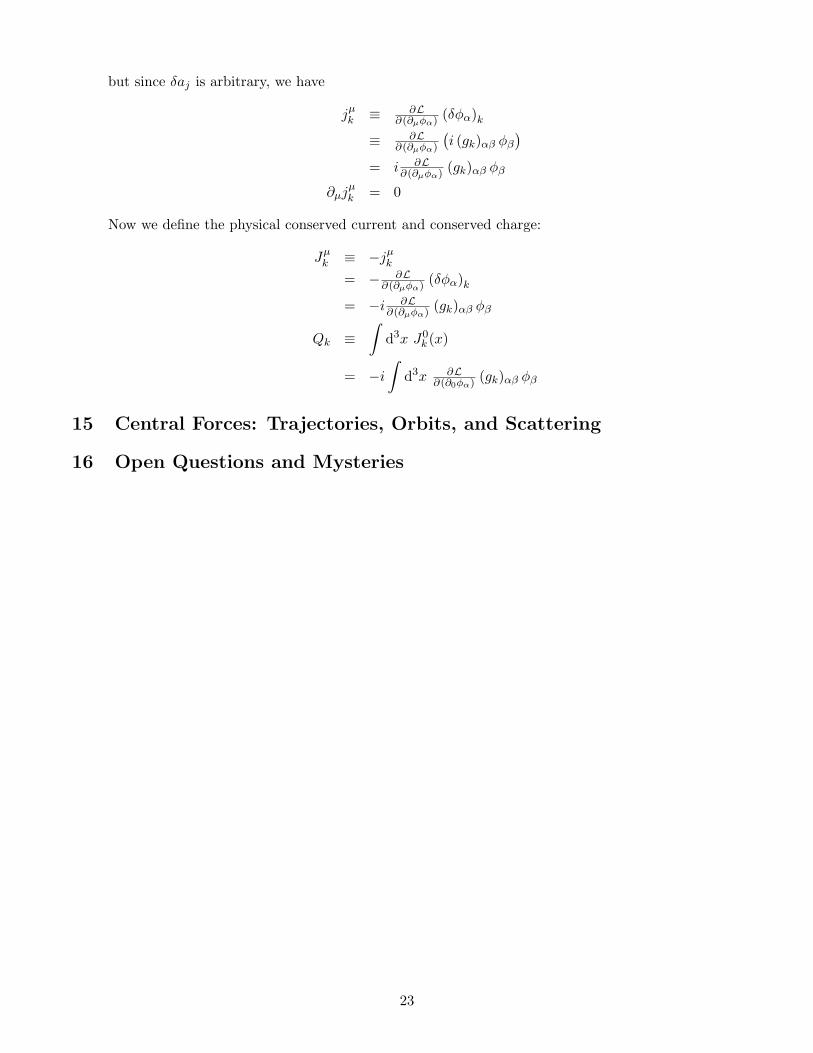
but since δaj is arbitrary, we have

jµk ≡ ∂L∂(∂µφα) (δφα)k

≡ ∂L∂(∂µφα)

(i (gk)αβ φβ

)= i ∂L

∂(∂µφα) (gk)αβ φβ

∂µjµk = 0

Now we define the physical conserved current and conserved charge:

Jµk ≡ −jµk= − ∂L

∂(∂µφα) (δφα)k

= −i ∂L∂(∂µφα) (gk)αβ φβ

Qk ≡∫

d3x J0k (x)

= −i∫

d3x ∂L∂(∂0φα) (gk)αβ φβ

15 Central Forces: Trajectories, Orbits, and Scattering

16 Open Questions and Mysteries

23

17 Class on Mechanics and Field Theory

17.1 Books to Use

• Goldstein: Classical Mechanics• Landau and Lifshitz: Mechanics• Davison Soper: Classical Field Theory• V.I. Arnold (A. Weinstein, and K. Vogtmann): Mathematical Methods of Classical Mechanics• Flanders: Differential Forms with Applications to the Physical Sciences• MTW: Gravitation (has interesting things to say about E&M and perhaps Mechanics)• Interesting references

− From Goldstein:

∗ F. Klein and A. Sommerfeld, Theorie des Kreisels, a monumental work on the theory of thetop. In Volume II, many pages are given to a thorough demolishing of the popular or elementary“derivations” of gyroscopic precession. The authors remark that it was the unsatisfactory natureof these derivations that led them to write the treatise!

17.2 Class Topics

Advanced Classical Mechanics and Classical Field Theory (and their relation to all subtopics of physics)from physical and mathematical perspectives• Lagrangian and Hamiltonian formalism

− Lagrangian: generalized coords (and momenta)− Hamiltonian: canonical coords (and momenta)− Legendre transformations, generating functions (physics versus math generating functions)− Canonical transformations (→ contact transformations, symplectomorphisms; Hamilton-Jacobi eqns,

conserved quantities)− Poisson Brackets, Symplectic Manifolds, Hamiltonian flow− and the relation to the many quantization schemes

• Theorems in classical mechanics

− Noether’s Thm− Liouville’s Thm, the fluctuation thm and proof for the second law of thermodynamics, Ehrenfest

thm, Lindblad eqn− Helmholtz Thm− (Stone-von Neumann thm)?

• Specific Problems:

− the Runge-Lenz vector and its quantum counterpart− Small-distance cuts-off in classical theories (e.g. viscosity, speed of sound, magnetic susceptibility)

and their relationship to cuts-off in QFT− (at atomic scales, where continuum description no longer applies)− (see Peskin and Schroeder pg 266)

• Continuum and fluid mechanics

24

• Dynamical systems: differential equations, bifurcation theory, and Hamiltonian systems; differentialdynamics, including hyperbolic theory and quasiperiodic dynamics; ergodic theory; low-dimensionaldynamics.

− Chaos and Ergodicity

• Asymptotic methods: Asymptotic Fundamental mathematics of asymptotic analysis, asymptotic ex-pansions of Fourier integrals, method of stationary phase. Watson lemma, method of steepest descent,uniform asymptotic expansions, elementary perturbation problems

17.3 Core Topics for Class, from Goldstein

Ch 1 Elementary PrinciplesCh 2 Variational Principles and Lagrange’s EqnsCh 6 Small OscillationsCh 8 Hamilton Eqns of MotionCh 9 Canonical TransformationsCh 12 Lagrangians / Hamiltonians for Fields / Continuous Systems

17.4 Investigate

Ch 10 . . .Ch 11 . . .• Landau and Lifshitz Mechanics

17.5 Take note of. . .

• pg ix

− Manipulation of tensors in non-Euclidean spaces (in Chs. 6 and 7)− Complex Minkowski space

• pg xi-xii

− the technique of action-angle variables is needed for the older quantum mechanics− the Hamilton-Jacobi eqn and the principle of least action provide the transition to wave mechanics− Poisson brackets and canonical transformations are invaluable in formulating the newer quantum

mechanics− classical mechanics affords the student an opportunity to master many of the mathematical tech-

niques necessary for quantum mechanics while still working in terms of the familiar concepts ofclassical physics

∗ the discussion of central force motion includes the kinematics of scattering and the clasicalsolution of scattering problems∗ . . . by the technique [of a unified mathematical treatment of rotations in terms of the eigen-

value problem for an orthogonal matrix] it becomes possible to include at an early stage thedifficult concepts of reflection operations and pseudotensor quantities . . . [and] “spinors” can beintroduced in connection with the properties of Cayley-Klein parameters.

25

References

[1] Herbert Goldstien: Classical Mechanics, Second Edition, Addison-Wesley (1980)

[2] Sean M. Carroll: Spacetime and Geometry: An Introduction to General Relativity, Addison-Wesley(2004)

[3] Davison E. Soper: Classical Field Theory, John Wiley & Sons, Inc. (1976)

26