Notes on Canonical FormsJohn Beachy, Spring 2007

Throughout these notes V will denote a finite dimensional vector space over afield F and T : V → V will be a linear transformation. Our goal is to choose a basisfor V in such a way that the corresponding matrix for T has as “simple” a form aspossible. We will try to come as close to a diagonal matrix as possible.

The notes will follow the terminology of Curtis in Linear Algebra: an introductoryapproach, as much as possible. The order of some results may be changed, and someproofs will be different.

22. BASIC CONCEPTS

Eigenvalues and eigenvectors

Definition 23.10: The linear transformation T is called diagonalizable if thereexists a basis for V with respect to which the matrix for T is a diagonal matrix.

Let’s look at what it means for the matrix of T to be diagonal. Recall that we getthe matrix by choosing a basis {u1,u2, . . . ,un}, and then entering the coordinatesof T (u1) as the first column, the coordinates of T (u2) as the second column, etc.The matrix is diagonal, with entries α1, α2, . . . , αn, if and only if the chosen basis hasthe property that T (ui) = αiui, for 1 ≤ i ≤ n. This leads to the definition of an“eigenvalue” and its corresponding “eigenvectors”.

Definition 22.7: A scalar α ∈ F is called an eigenvalue of T if there exists anonzero vector v ∈ V such that

T (v) = αv .

In this case, v is called an eigenvector of T belonging to the eigenvalue α.

As noted above, the significance of this definition is that there is a diagonal matrixthat represents T if and only if there exists a basis for V that consists of eigenvectorsof T . Note that the terms characteristic value and eigenvalue are used synonymously,as are the terms characteristic vector and eigenvector.

If v1 and v2 are eigenvectors belonging to the eigenvalue α of T , then so is anynonzero vector a1v1 + a2v2, since

T (a1v1 + a2v2) = a1T (v1) + a2T (v2) = a1αv1 + a2αv2 = α(a1v1 + a2v2) .

For each eigenvalue α of T , the set of eigenvectors that belong to it, together withthe zero vector, forms a subspace.

1

In finding eigenvectors v with T (v) = αv, it is often easier to use the equivalentcondition [T − α1V ](v) = 0, where 1V is the identity mapping on V . Then theeigenvectors corresponding to an eigenvalue α are precisely the nonzero vectors in thenull space n(T − α1V ) (which is the same as the kernel of T − α1V ).

Definition: If α is an eigenvalue of T , then the null space n(T −α1V ) is called theeigenspace of α.

For example, 0 is an eigenvalue of T if and only if T is not one-to-one. In thiscase the eigenspace of 0 is just the null space of T .

In searching for eigenvectors there is yet another point of view. If T (v) = αv, thenT (λv) = αλv, showing that the vectors in the one dimensional subspace spanned byv are all mapped by T back into the same one dimensional subspace. For example,if V = R3, then to find eigenvectors of T we need to look for lines through the originthat are mapped by T back into themselves. This point of view leads to an importantdefinition.

Definition 23.1: A subspace W of V is called a T -invariant subspace if T (w) ∈ W ,for all w ∈ W .

With this terminology, a nonzero vector v is an eigenvector of T if and only if itbelongs to a one-dimensional invariant subspace of V .

It is easy to check that the null space of T and the range of T are T -invariantsubspaces. An interesting case occurs when T is a projection, with T 2 = T . Then wehave shown that V = n(T )⊕T (V ), and so V is a direct sum of T -invariant subspaces.It is important to know that if α is an eigenvalue of T , then the eigenspace of α isa T -invariant subspace. This follows directly from the fact that if v is an eigenvaluebelonging to α, then so is T (v), since T (v) = αv.

We have been considering the eigenvectors belonging to a given eigenvalue. Buthow do we find the eigenvalues? From the definition of an eigenvalue, the scalar α isan eigenvalue if and only if n(T − α1V ) 6= 0. This allows us to conclude that α is aneigenvalue if and only if the determinant D(T − α1V ) is zero. Then we can find theeigenvalues of T as the zeros of the polynomial equation D(x1V − T ) = 0. Thus wemust choose a basis for V and then find the matrix A which represents T relative tothe basis. Finally, we must solve the equation D(xI −A) = 0, where I is the identitymatrix.

Definition 24.6: If A is an n × n matrix, then the polynomial f(x) = D(xI − A)is called the characteristic polynomial of A.

2

We want to be able to talk about the characteristic polynomial of a linear trans-formation, independently of the basis chosen for its matrix representation. The nextproposition shows that this is indeed possible (see page 205 of Curtis).

Proposition: Similar matrices have the same characteristic polynomial.

Proof. Let A, B be n×n matrices. If there exists an invertible n×n matrix S withB = S−1AS, then

D(xI −B) = D(xI − S−1AS) = D(xS−1S − S−1AS)

= D(S−1xIS − S−1AS) = D(S−1(xI − A)S)

= D(S−1)D(xI − A)D(S) = D(xI − A) .

This completes the proof. �

Definition 24.6′: Let A be a matrix of T with respect to some basis of V . Thenthe polynomial f(x) = D(xI − A) is called the characteristic polynomial of T .

We have already noted that α is an eigenvalue of T if and only if D(T −α1V ) = 0.We can state the final theorem of the section in a slightly different way than Curtisdoes. Its proof should be clear from the above discussion.

Theorem 22.10: The eigenvalues of T are the zeros of its characteristic polynomial.

In practice, there are many applications in which it is important to find the eigen-values of a matrix. Using the characteristic polynomial of the matrix turns out to beimpractical, and so various computational techniques have been developed. These arebeyond the scope of this course, but you can get some idea about them from Kolmanand Hill (the Math 240 book).

It turns out that we need to work not only with T but with combinations ofpowers of T . In particular, if we have any polynomial with coefficients in F , there isa corresponding linear transformation found by substituting T into the polynomial.The only problem is what to do with the constant terms, since the final result mustbe a linear transformation.

Example 1: If A =

[a bc d

], then its characteristic polynomial is

f(x) = D(xI−A) =

∣∣∣∣ x− a −b−c x− d

∣∣∣∣ = (x−a)(x−d)−bc = x2−(a+d)x+(ad−bc) .

Note that f(x) involves the trace and determinant of A. Curtis does this calculationin Example A, on page 187, and then writes out the characteristic polynomial of a3× 3 matrix in Example B, on page 188.

3

Definition 22.1: Let f(x) = amxm + . . . + a1x + a0 be a polynomial in F [x]. Thenf(T ) denotes the linear transformation

f(T ) = amTm + . . . + a1T + a01V : V → V ,

where 1V is the identity on V . Similarly, if A is an n× n matrix, then f(A) denotesthe n× n matrix

f(A) = amAm + . . . + a1A + a0I ,

where I is the n× n identity matrix.If f(T ) is the zero transformation on V , we say that T satisfies the polynomial

f(x). Similarly, a matrix A satisfies the polynomial f(x) if f(A) is the zero matrix.

Before proving the next result, we need to make an observation about the actionof powers of T on eigenvectors. Suppose that v ∈ V and T (v) = αv for some scalarα. Then for any polynomial anx

n + . . . + a1x + a0 we have

[anTn + . . . + a1T + a01v](v) = anT

n(v) + . . . + a1T (v) + a0(v)

= anαnv + . . . + a1αv + a0v

= (anαn + . . . + a1α + a0)v

or equivalently, [f(T )](v) = f(α) · v.The proof of the next theorem is a slick one, using the above paragraph. It

makes use of the functions fi that turn up in the proof of the Lagrange interpolationformula. Note that Curtis has a proof that is easier to remember, and maybe easierto understand.

Theorem 22.8: Let v1,v2, . . . ,vr be eigenvectors belonging to the distinct eigen-values α1, α2, . . . , αr of T . Then the vectors v1,v2, . . . ,vr are linearly independent.

Proof. It is possible to choose polynomials fi(x) such that

fi(αj) =

{1 if i = j0 if i 6= j.

If∑r

j=1 λjvj = 0, then multiplying by fi(T ) gives

0 = [fi(T )](∑r

j=1 λjvj) =∑r

j=1 λjfi(αj) · vj = λivi

which shows that λi = 0 for all i. Thus the given eigenvectors are linearly indepen-dent. �

Remember that diagonalizing a matrix is equivalent to finding a basis consistingof eigenvectors. We need to recall the procedure in Math 240 for attempting to

4

diagonalize an n×n matrix A. We first find the eigenvalues of A by finding the zerosof the characteristic polynomial f(x). These correspond to linear factors of f(x), andif we cannot factor f(x) into a product of linear factors, then we cannot possibly findenough linearly independent eigenvectors, so A is not diagonalizable.

If we find that there are enough eigenvalues, then for each eigenvalue α, we solvethe system of equations (A−αI)x = 0 to find a basis for the corresponding eigenspace.The next problem is that some of the zeros may have multiplicity greater than 1,corresponding to linear factors of degree greater than 1. If α is not a repeated root,then the solution space is one dimensional and we can easily find a basis, which givesthe eigenvector corresponding to α. If α is a repeated root, say of multiplicity m,then we need m linearly independent eigenvectors belonging to α. In order for thisto occur, we need the nullity of A− αI to be equal to m.

I think that this review is enough to prove the following theorem. Just rememberthat the eigenspace of eigenvectors belonging to αi is the null space n(T − αi1V ).

Theorem: Let α1, . . . , αs be the distinct eigenvalues of T , and let Vi = n(T −αi1v).The following are equivalent.

(1) T is diagonalizable;

(2) the characteristic polynomial of T is f(x) = (x − α1)e1 · · · (x − αs)

es, anddim(Vi) = ei, for all i;

(3) dim(V1) + . . . + dim(Vs) = dim(V ).

Proof. It is easy to see that (1) implies (2), since we can compute the characteristicpolynomial using a diagonal matrix that represents T .

We have (2) implies (3) since the degree of f(x) is equal to dim(V ).Finally, if (3) holds then we can choose a basis for each of the nonzero eigenspaces

Vi, and then by Theorem 22.8, the union of these bases must be a basis for V . Sincewe have found a basis of eigenvectors, the corresponding matrix is diagonal, and thusT is diagonalizable. �

From Math 240, you are probably familiar with the following result (page 274 ofCurtis). The proof requires a deeper analysis of matrices over the complex numbers,so we will almost certainly not have time to prove it.

Theorem 31.12: Let V be a finite dimensional vector space over the field R of realnumbers. If T ∈ L(V, V ) is symmetric, then there exists an orthonormal basis for Vconsisting of eigenvectors of T .

5

The minimal polynomial for T

We have shown that L(V, V ) is a vector space, and since it is isomorphic to thevector space Mn(F ) of n × n matrices, it has dimension n2. If we consider theset I, T, . . . , T n2

in L(V, V ), we have n2 + 1 elements, so they cannot be linearlyindependent. Thus there is some linear combination a0I + a1T + . . . + an2+1T

n2that

equals the zero function. This is the proof given by Curtis that every T ∈ L(V, V )satisfies some polynomial of degree ≤ n2. Knowing that there is some polynomialthat T satisfies, we can find a polynomial of minimal degree that T satisfies, and thenwe can divide by its leading coefficient to obtain a monic polynomial. We will verifythe uniqueness of this “minimal polynomial” in Theorem 22.3.

Definition 22.4: The monic polynomial m(x) of minimal degree such that m(T ) = 0is called the minimal polynomial of T .

Theorem 22.3:(a) The minimal polynomial of T exists and is unique.(b) If m(x) is the minimal polynomial of T and f(x) is any polynomial with

f(T ) = 0, then m(x) is a factor of f(x).

Proof. Let m(x) be a monic polynomial of minimal degree such that m(T ) = 0.Suppose that f(x) is any polynomial with f(T ) = 0. The division algorithm holdsfor polynomials with coefficients in the field F , so it is possible to write f(x) =q(x)m(x) + r(x), where either r(x) = 0 or deg(r(x)) < deg(m(x)). If r(x) is nonzero,then we have r(T ) = f(T ) − q(T )m(T ) = 0. We can divide r(x) by its leadingcoefficient to obtain a monic polynomial satisfied by T , and then this contradicts thechoice of m(x) as a monic polynomial of minimal degree satisfied by T . We concludethat the remainder r(x) is zero, so f(x) = q(x)m(x) and m(x) is thus a factor of f(x).

If h(x) is another monic polynomial of minimal degree with h(T ) = 0, then by thepreceding paragraph m(x) is a factor of h(x), and h(x) is a factor of m(x). Since bothare monic polynomials, this forces h(x) = m(x), showing that the minimal polynomialis unique. �

We need to investigate the relationship between the characteristic polynomial andthe minimal polynomial of T . They are closely related, and the interplay betweenthem will help to determine the best form for a matrix for T . We now return toeigenvalues and eigenvectors, showing that the minimal polynomial can also be usedto find the eigenvalues of T .

Proposition: The characteristic and minimal polynomials of a linear transforma-tion have the same zeros (except for multiplicities).

6

Proof. Let m(x) be the minimal polynomial of T . We need to prove that m(α) = 0if and only if α is an eigenvalue of T .

First assume that m(α) = 0. Then m(x) = (x−α)q(x) for some q(x) ∈ F [x], sincezeros correspond to linear factors. Since deg(q(x)) < deg(m(x)), we have q(T ) 6= 0,because m(x) has minimal degree among polynomials satisfied by T . Therefore thereexists u ∈ V with [q(T )](u) 6= 0. Letting v = [q(T )](u) gives

[T − α1V ](v) = [(T − α1V )q(T )](u) = [m(T )](u) = 0

and thus v is an eigenvector of T with eigenvalue α.Conversely, assume that α is an eigenvalue of T , say T (v) = αv for some v 6= 0.

Then m(α) · v = [m(T )](v) = 0 implies that m(α) = 0 since v 6= 0. �

A stronger statement than the above proposition is that the minimal polynomialof T is a factor of the characteristic polynomial of T . This follows from the Cayley-Hamilton theorem, which shows that any matrix satisfies its characteristic polynomial.This also gives an easier proof of part of the previous proposition, since the zeros ofa polynomial m(x) are automatically zeros of any multiple m(x)q(x).

Theorem 24.8 [Cayley-Hamilton]: If f(x) is the characteristic polynomial of ann× n matrix A, then f(A) = 0.

Proof. Let f(x) = D(xI − A) = a0 + a1x + . . . + xn, and let B(x) be the matrixwhich is the adjoint of xI − A. The entries of B(x) are cofactors of xI − A, and sothey are polynomials of degree ≤ n− 1, which allows us to factor out powers of x toget B(x) = B0 +B1x+ . . .+Bn−1x

n−1, for some n×n matrices B0, B1, . . . , Bn−1. Bydefinition of the adjoint, (xI − A) ·B(x) = D(xI − A) · I, or

(xI − A)(B0 + B1x + . . . + Bn−1xn−1) = (a0 + a1x + . . . + xn) · I

If we equate coefficients of x and then multiply by increasing powers of A we obtain

−AB0 = a0I and then −AB0 = a0I

B0 − AB1 = a1I AB0 − A2B1 = a1A...

...

Bi−1 − ABi = aiI AiBi−1 − Ai+1Bi = ai−1Ai

......

Bn−1 = I AnBn−1 = An

If we add the right hand columns, we get 0 = a0I + a1A + . . . + An, or simplyf(A) = 0. �

7

Curtis gives a special case of The Cayley-Hamilton theorem in Theorem 24.8, andthen outlines a proof of the general case in Exercise 8 on page 226. The above proofis easier, so it makes sense to present it here, since we can use it immediately.

As a corollary of the Cayley-Hamilton theorem, we can now see that the minimalpolynomial of T has degree ≤ n, Note that in the next section Curtis characterizesdiagonalizable matrices in terms of their minimal polynomials: A is diagonalizable ifand only if its minimal polynomial has the form m(x) = (x− α1) · · · (x− αs), whereαi 6= αj for i 6= j. That is, A is diagonalizable if and only if its minimal polynomialis a product of linear factors, with no repetitions.

EXERCISES

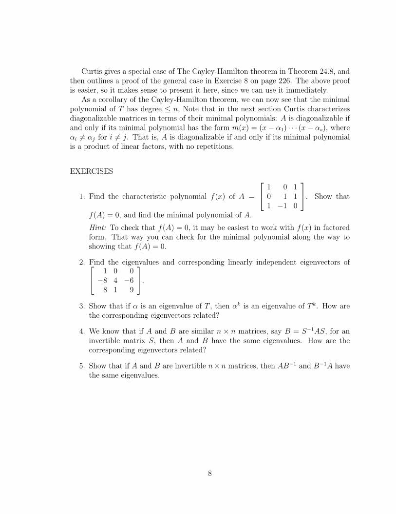
1. Find the characteristic polynomial f(x) of A =

1 0 10 1 11 −1 0

. Show that

f(A) = 0, and find the minimal polynomial of A.

Hint: To check that f(A) = 0, it may be easiest to work with f(x) in factoredform. That way you can check for the minimal polynomial along the way toshowing that f(A) = 0.

2. Find the eigenvalues and corresponding linearly independent eigenvectors of 1 0 0−8 4 −6

8 1 9

.

3. Show that if α is an eigenvalue of T , then αk is an eigenvalue of T k. How arethe corresponding eigenvectors related?

4. We know that if A and B are similar n × n matrices, say B = S−1AS, for aninvertible matrix S, then A and B have the same eigenvalues. How are thecorresponding eigenvectors related?

5. Show that if A and B are invertible n×n matrices, then AB−1 and B−1A havethe same eigenvalues.

8

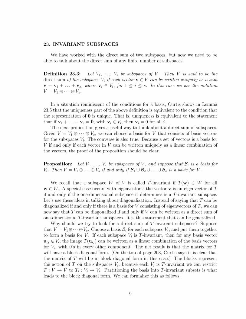
23. INVARIANT SUBSPACES

We have worked with the direct sum of two subspaces, but now we need to beable to talk about the direct sum of any finite number of subspaces.

Definition 23.3: Let V1, . . ., Vs be subspaces of V . Then V is said to be thedirect sum of the subspaces Vi if each vector v ∈ V can be written uniquely as a sumv = v1 + . . . + vs, where vi ∈ Vi, for 1 ≤ i ≤ s. In this case we use the notationV = V1 ⊕ · · · ⊕ Vs.

In a situation reminiscent of the conditions for a basis, Curtis shows in Lemma23.5 that the uniqueness part of the above definition is equivalent to the condition thatthe representation of 0 is unique. That is, uniqueness is equivalent to the statementthat if v1 + . . . + vs = 0, with vi ∈ Vi, then vi = 0 for all i.

The next proposition gives a useful way to think about a direct sum of subspaces.Given V = V1 ⊕ · · · ⊕ Vs, we can choose a basis for V that consists of basis vectorsfor the subspaces Vi. The converse is also true. Because a set of vectors is a basis forV if and only if each vector in V can be written uniquely as a linear combination ofthe vectors, the proof of the proposition should be clear.

Proposition: Let V1, . . ., Vs be subspaces of V , and suppose that Bi is a basis forVi. Then V = V1 ⊕ · · · ⊕ Vs if and only if B1 ∪ B2 ∪ . . . ∪ Bs is a basis for V .

We recall that a subspace W of V is called T -invariant if T (w) ∈ W for allw ∈ W . A special case occurs with eigenvectors: the vector v is an eigenvector of Tif and only if the one-dimensional subspace it determines is a T -invariant subspace.Let’s use these ideas in talking about diagonalization. Instead of saying that T can bediagonalized if and only if there is a basis for V consisting of eigenvectors of T , we cannow say that T can be diagonalized if and only if V can be written as a direct sum ofone-dimensional T -invariant subspaces. It is this statement that can be generalized.

Why should we try to look for a direct sum of T -invariant subspaces? Supposethat V = V1⊕· · ·⊕Vs. Choose a basis Bi for each subspace Vi, and put them togetherto form a basis for V . If each subspace Vi is T -invariant, then for any basis vectoruij ∈ Vi, the image T (uij) can be written as a linear combination of the basis vectorsfor Vi, with 0’s in every other component. The net result is that the matrix for Twill have a block diagonal form. (On the top of page 203, Curtis says it is clear thatthe matrix of T will be in block diagonal form in this case.) The blocks representthe action of T on the subspaces Vi; because each Vi is T -invariant we can restrictT : V → V to Ti : Vi → Vi. Partitioning the basis into T -invariant subsets is whatleads to the block diagonal form. We can formalize this as follows.

9

Proposition: Let V1, . . ., Vs be T -invariant subspaces with V = V1⊕· · ·⊕Vs. If wechoose a basis Bi for each Vi, then the matrix of T relative to the basis B1∪B2∪. . .∪Bs

has block diagonal form

A1 0

A2

. . .

0 As

.

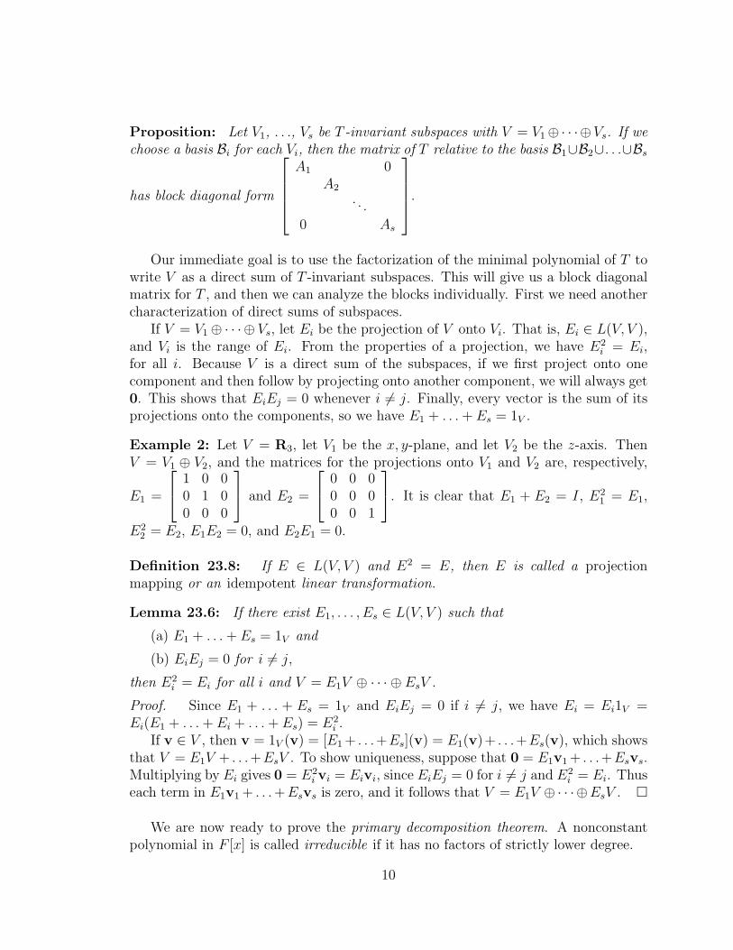
Our immediate goal is to use the factorization of the minimal polynomial of T towrite V as a direct sum of T -invariant subspaces. This will give us a block diagonalmatrix for T , and then we can analyze the blocks individually. First we need anothercharacterization of direct sums of subspaces.

If V = V1⊕ · · · ⊕ Vs, let Ei be the projection of V onto Vi. That is, Ei ∈ L(V, V ),and Vi is the range of Ei. From the properties of a projection, we have E2

i = Ei,for all i. Because V is a direct sum of the subspaces, if we first project onto onecomponent and then follow by projecting onto another component, we will always get0. This shows that EiEj = 0 whenever i 6= j. Finally, every vector is the sum of itsprojections onto the components, so we have E1 + . . . + Es = 1V .

Example 2: Let V = R3, let V1 be the x, y-plane, and let V2 be the z-axis. ThenV = V1 ⊕ V2, and the matrices for the projections onto V1 and V2 are, respectively,

E1 =

1 0 00 1 00 0 0

and E2 =

0 0 00 0 00 0 1

. It is clear that E1 + E2 = I, E21 = E1,

E22 = E2, E1E2 = 0, and E2E1 = 0.

Definition 23.8: If E ∈ L(V, V ) and E2 = E, then E is called a projectionmapping or an idempotent linear transformation.

Lemma 23.6: If there exist E1, . . . , Es ∈ L(V, V ) such that

(a) E1 + . . . + Es = 1V and

(b) EiEj = 0 for i 6= j,

then E2i = Ei for all i and V = E1V ⊕ · · · ⊕ EsV .

Proof. Since E1 + . . . + Es = 1V and EiEj = 0 if i 6= j, we have Ei = Ei1V =Ei(E1 + . . . + Ei + . . . + Es) = E2

i .If v ∈ V , then v = 1V (v) = [E1 + . . .+Es](v) = E1(v)+ . . .+Es(v), which shows

that V = E1V + . . .+EsV . To show uniqueness, suppose that 0 = E1v1 + . . .+Esvs.Multiplying by Ei gives 0 = E2

i vi = Eivi, since EiEj = 0 for i 6= j and E2i = Ei. Thus

each term in E1v1 + . . .+Esvs is zero, and it follows that V = E1V ⊕ · · ·⊕EsV . �

We are now ready to prove the primary decomposition theorem. A nonconstantpolynomial in F [x] is called irreducible if it has no factors of strictly lower degree.

10

We begin with the minimal polynomial m(x) of T , and factor it completely intoirreducible factors, to get m(x) = p1(x)e1p2(x)e2 · · · ps(x)es . We then consider thelinear transformations pi(T )ei , and their null spaces Vi = n(pi(T )ei). Each Vi is T -invariant, since if w ∈ Vi, then T (w) ∈ Vi because [pi(T )ei ](T (w)) = T (pi(T )ei(w)) =T (0) = 0. (See Lemma 23.2 in Curtis.) Note that if pi(x)ei happens to be a linearfactor x− α, then Vi = n(T − α1V ) is the eigenspace of α.

Theorem 23.9: Let m(x) = p1(x)e1p2(x)e2 · · · ps(x)es be the minimal polynomial ofT , factored completely as a product of powers of distinct monic irreducible polynomialspi(x). For each i, let Vi be the null space n(pi(T )ei).

Then V = V1⊕ · · · ⊕ Vs, showing that V is a direct sum of T -invariant subspaces.

Proof. Let qi(x) = m(x)/pi(x)ei , so that qi(x) contains all but one of the irreduciblefactors of m(x). Note that if i 6= j, then our definition guarantees that qi(x)qj(x) hasm(x) as a factor. The polynomials qi(x), for 1 ≤ i ≤ s, have no irreducible factor incommon, and so since they are relatively prime there must exist polynomials ai(x)with

∑si=1 ai(x)qi(x) = 1.

Let Ei = ai(T )qi(T ). Then∑s

i=1 Ei = 1V , and EiEj = 0 if i 6= j since EiEj =m(T )q(T ) for some polynomial q(x). Thus V = EiV ⊕ · · · ⊕ EsV by Lemma 23.6.

It remains to show that EiV = Vi, for all i. To prove that EiV ⊆ Vi, let v ∈ EiV .Then v = [qi(T )](w), for some w ∈ V , and so [pi(T )ei ](v) = [pi(T )ei ](qi(T )w) =[pi(T )eiqi(T )](w) = m(T )w = 0.

To prove that Vi ⊆ EiV , let v ∈ Vi. Then [qj(T )](v) = 0, since qj(T ) has pi(T )ei

as a factor. But 1V =∑s

j=1 Ej, so v = [∑s

j=1 Ej](v) = Ei(v) ∈ EiV . �

Theorem 23.11: The linear transformation T is diagonalizable if and only if itsminimal polynomial is a product of distinct linear factors.

Proof. If T is diagonalizable, we can compute its minimal polynomial using adiagonal matrix, and then it is clear that we just need one linear factor for each ofthe distinct entries along the diagonal.

Conversely, let the minimal polynomial of T be m(x) = (x−α1)(x−α2) · · · (x−αs).Then V is a direct sum of the null spaces n(T −αi1V ), which shows that there existsa basis for V consisting of eigenvectors, and so T is diagonalizable.. �

Example 3: We can now show that Example 2 gives a model for all idempotentlinear transformations, in the following sense. If E2 = E, then E satisfies the poly-nomial x2 − x, so its minimal polynomial is x(x − 1) or x or x − 1. It follows fromTheorem 23.11 that E is diagonalizable, so it is possible to find a basis for V suchthat the corresponding matrix for E is diagonal, with 1’s and/or 0’s down the maindiagonal, as in Example 2.

11

24. TRIANGULAR FORM

Definition: The linear transformation T is called triangulable if there exists a basisfor V such that the matrix of T relative to the basis is an upper triangular matrix.

Lemma: Let W be any proper T -invariant subspace of V . If the minimal polynomialof T is a product of linear factors, then there exists v 6∈ W such that [T−α1V ](v) ∈ Wfor some eigenvalue α of T .

Proof. Let m(x) be the minimal polynomial of T , and let u ∈ V be any vectorwhich is not in W . Since m(T ) = 0 we certainly have [m(T )](u) ∈ W . Let p(x) bea monic polynomial of minimal degree with [p(T )](u) ∈ W . An argument similar tothat for the minimal polynomial shows that p(x) is a factor of every polynomial f(x)with the property that [f(T )](u) ∈ W . (See Lemma 25.4 in Curtis.) In particular,p(x) is a factor of m(x), and so by assumption it is a product of linear factors.

Suppose that x − α is a linear factor of p(x), say p(x) = (x − α)q(x) for someq(x) ∈ F [x]. Note that α is a eigenvalue of T since it is a zero of m(x). Thendeg(q(x)) < deg(p(x)), and so v = [q(T )](u) 6∈ W , but

[T − α1V ](v) = [T − α1V ](q(T )u) = [(T − α1V )q(T )](u) = [p(T )](u)

and this element belongs to W . �

Theorem 24.1: The linear transformation T is triangulable if and only if theminimal polynomial m(x) of T is a product of linear factors.

Proof. If T has a matrix that is upper triangular, then its characteristic polynomialis a product of linear factors, which guarantees that its minimal polynomial has thesame property.

To prove the converse, choose a basis for V as follows. Let u1 be a eigenvectorwith eigenvalue α1. Since the subspace W1 spanned by u1 is T -invariant, we canapply the previous lemma to obtain a vector u2 6∈ W1 with [T − α21V ](u2) ∈ W1, forsome eigenvalue α2 of T . (We are not claiming that α2 is different from α1.) ThenT (u2) = α2u2 + w1, where w1 ∈ W1. Next let W2 be the subspace spanned by u1

and u2. Since T maps the basis for W2 back into W2, the subspace W2 is T -invariantand we can repeat the argument. Thus T (ui) = αiui + wi−1, where wi−1 belongs tothe subspace spanned by {u1, . . . ,ui−1}. It follows that the matrix for T relative tothe basis which has been chosen is an upper triangular matrix. �

If a matrix A is upper triangular, it is easy to find its characteristic polynomial.A similar statement can be made about matrices in block diagonal form. Since thedeterminant of a matrix in block diagonal form is the product of the determinants

12

of the blocks, the characteristic polynomial of

A1 0. . .

0 As

is the product of the

characteristic polynomials of the blocks Ai. The corresponding statement for lineartransformations is that if V is a direct sum V = V1⊕· · ·⊕Vs of T -invariant subspaces,then we can write the characteristic polynomial of T as a product of the characteristicpolynomials of the linear transformations Ti : Vi → Vi that are the restriction of T toVi.

We now return to Theorem 23.9, and let Ti be the restriction of T to Vi. Letmi(x) be the minimal polynomial of Ti. Then mi(x) is a divisor of pi(x)ei sincepi(T )ei = 0 on Vi. On the other hand, mi(T )fi(T ) = 0 since fi(T )Vj = 0 for i 6= jwhile mi(T )Wi = 0. This implies that the minimal polynomial m(x) of T is a divisorof mi(x)fi(x), and then pi(x)ei must be a divisor of mi(x). It follows that the minimalpolynomial of Ti is mi(x) = pi(x)ei .

EXERCISES

1. Let A = [aij] be an n × n matrix with characteristic polynomial f(x) = xn +an−1x

n−1 + . . . + a1x + a0. By substituting x = 0, show that a0 = ±D(A), forthe determinant D(A) of A.

2. Let A = [aij] be an n × n matrix with characteristic polynomial f(x) = xn +an−1x

n−1 + . . . + a1x + a0. Use induction to show that f(x) = (x− a11) · · · (x−ann) + q(x), where q(x) has degree at most n − 2. Then show that −an−1 isequal to the trace tr(A) of A.

3. Let f(x) = xn + an−1xn−1 + . . . + a1x + a0 ∈ F [x]. The companion matrix of

f(x) is the matrix

A =

0 0 0 · · · 0 −a0

1 0 0 · · · 0 −a1

0 1 0 · · · 0 −a2...

......

......

0 0 0 · · · 0 −an−2

0 0 0 · · · 1 −an−1

. Show that the characteristic polynomial of

A is f(x), and thus f(A) = 0 by the Cayley-Hamilton theorem.

Hint: Find the determinant by expanding by cofactors along the last column.

13

25. JORDAN CANONICAL FORM

Definition 25.17: The matrix A is said to be in Jordan form if it satisfies thefollowing conditions.

(i) It must be in block diagonal form, where each block has a fixed scalar on themain diagonal and 1’s or 0’s on the superdiagonal. These blocks are called the primaryblocks of A.

(ii) The scalars for different primary blocks must be distinct.

(iii) Each primary block must be made up of secondary blocks with a scalar onthe diagonal and only 1’s on the superdiagonal. These blocks must be in order ofdecreasing size (moving down the main diagonal).

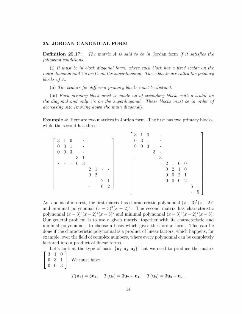
Example 4: Here are two matrices in Jordan form. The first has two primary blocks,while the second has three.

3 1 0 ·0 3 1 ·0 0 3 ·

3 1· · · 0 3

2 1 · ·0 2· 2 1· 0 2

3 1 0 ·0 3 1 ·0 0 3 ·

3 ·· · · · 3

2 1 0 00 2 1 00 0 2 10 0 0 2

5 ·· 5

As a point of interest, the first matrix has characteristic polynomial (x− 3)5(x− 2)4

and minimal polynomial (x − 3)3(x − 2)2. The second matrix has characteristicpolynomial (x− 3)5(x− 2)4(x− 5)2 and minimal polynomial (x− 3)3(x− 2)4(x− 5).Our general problem is to use a given matrix, together with its characteristic andminimal polynomials, to choose a basis which gives the Jordan form. This can bedone if the characteristic polynomial is a product of linear factors, which happens, forexample, over the field of complex numbers, where every polynomial can be completelyfactored into a product of linear terms.

Let’s look at the type of basis {u1,u2,u3} that we need to produce the matrix 3 1 00 3 10 0 3

. We must have

T (u1) = 3u1, T (u2) = 3u2 + u1, T (u3) = 3u3 + u2 .

14

We can rewrite this in the following way:

[T − 31V ](u1) = 0, [T − 31V ](u2) = u1, [T − 31V ](u3) = u2 .

This also implies that

[T − 31V ](u1) = 0, [T − 31V ]2(u2) = 0, [T − 31V ]3(u3) = 0 .

In this case u2 is called a generalized eigenvector of degree 2, and u3 is called ageneralized eigenvector of degree 3.

Definition: Let W1 ⊆ W2 be subspaces of V . Let B be a basis for W1. Any set B′

of vectors such that B ∪ B′ is a basis for W2 is called a complementary basis for W1

in W2.

Lemma: Let L : V → V be a linear transformation. Let {u1, . . . ,uk} be a comple-mentary basis for n(Lm) in n(Lm+1). Then {L(u1), . . . , L(uk)} is part of a comple-mentary basis for n(Lm−1) in n(Lm).

Proof. Since ui ∈ n(Lm+1), we have Lm+1(ui) = 0, so Lm(L(ui)) = 0, and thereforeL(ui) ∈ n(Lm). If

∑ki=1 ciL(ui) ∈ n(Lm−1), then

Lm

(k∑

i=1

ciui

)= Lm−1

(k∑

i=1

ciL(ui)

)= 0 .

This implies that∑k

i=1 ciui ∈ n(Lm), and then ci = 0 for all i since {u1, . . . ,uk} isa complementary basis for n(Lm) in n(Lm+1). This shows that L(u1), . . . , L(uk) arelinearly independent and also linearly independent of any vectors in n(Lm−1), so theyare part of a complementary basis for n(Lm−1) in n(Lm). �

Theorem [Jordan canonical form]: If the characteristic polynomial of T is aproduct of linear factors, then it is possible to find a matrix representation for Twhich has Jordan form.

In particular, suppose that f(x) = (x − α1)m1 · · · (x − αs)

ms is the characteristicpolynomial of T and suppose that m(x) = (x−α1)

e1 · · · (x−αs)es is the minimal poly-

nomial of T . Then the matrix for T has primary blocks of size mi×mi correspondingto each eigenvalue αi, and in each primary block the largest secondary block has sizeei × ei.

Proof. By using Theorem 23.9 (the primary decomposition theorem) we can obtaina block diagonal matrix, and then we can deal with each block separately. Thisreduces the proof to the case in which the characteristic polynomial is (x− α)m andthe minimal polynomial is (x− α)r.

15

Choose a complementary basis u1,u2, . . . ,uk for n((T−α1V )r−1) in n((T−α1V )r).By the preceding lemma, the vectors

[T − α1V ]r−1(u1), . . . , [T − α1V ](u1), u1,

[T − α1V ]r−1(u2), . . . , [T − α1V ](u2), u2, . . . . . .

[T − α1V ]r−1(uk) . . . , [T − α1V ](uk), uk,

are linearly independent. Starting with [T − α1V ](u1), . . . , [T − α1V ](uk) we findadditional vectors w1, . . . ,wt to complete a complementary basis for n((T −α1V )r−2)in n((T − α1V )r−1) . Then we also include

[T − α1V ]r−2(w1), . . . , [T − α1V ](w1) ,

and so on. We then consider n((T −α1V )r−2), etc., and continue this procedure untilwe have found a basis for the generalized eigenspace n((T − α1V )r.

Finally we must compute the matrix of T with respect to the basis we have chosen.It is useful to write T = α1V + (T − α1V ). Then, for example,

T ([T − α1V ]j(ui)) = c[T − α1V ]j(ui) + [T − α1V ]j+1(ui)

and it follows rather easily that the basis we have chosen leads to a matrix in Jordanform. �

We have given a direct proof that shows that all matrices over an algebraicallyclosed field (such as C) can be put into Jordan form. This proof does not make use ofthe more general rational canonical form that is developed by Curtis, which appliesto all matrices.

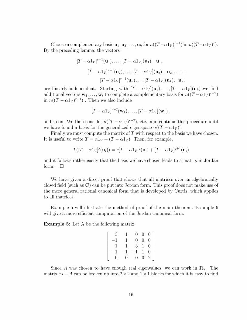
Example 5 will illustrate the method of proof of the main theorem. Example 6will give a more efficient computation of the Jordan canonical form.

Example 5: Let A be the following matrix.3 1 0 0 0

−1 1 0 0 01 1 3 1 0

−1 −1 −1 1 00 0 0 0 2

Since A was chosen to have enough real eigenvalues, we can work in R5. The

matrix xI−A can be broken up into 2×2 and 1×1 blocks for which it is easy to find

16

the determinant. The only work we need to do to find the characteristic polynomialf(x) is to evaluate∣∣∣∣ x− 3 −1

1 x− 1

∣∣∣∣ = (x− 3)(x− 1) + 1 = x2 − 4x + 4 = (x− 2)2 .

We conclude that f(x) = (x − 2)5. To find the minimal polynomial of A, since weknow it must be a power of (x − 2), we just need to find the first power of A − 2Iwhich gives the zero matrix.

(A− 2I)2 =

1 1 0 0 0

−1 −1 0 0 01 1 1 1 0

−1 −1 −1 −1 00 0 0 0 0

1 1 0 0 0−1 −1 0 0 0

1 1 1 1 0−1 −1 −1 −1 0

0 0 0 0 0

=

0 0 0 0 00 0 0 0 00 0 0 0 00 0 0 0 00 0 0 0 0

This tells us that the minimal polynomial is (x−2)2. The next step is to find n(A−2I),the eigenspace of 2. The generalized eigenspace n(A− 2I)2 is all of R5.

We first give the block upper triangular form of the matrix obtained by choosinga basis for the invariant subspace consisting of all eigenvectors. Solving the system(A − 2I)x = 0 gives x2 = −x1, x4 = −x3. We can choose a basis for the eigenspacein the usual way, by considering x1, x3, x5 as independent variables. We then extendit to a basis for the whole space, by choosing two more linearly independent vectors.This gives us the following basis: u1 = (1,−1, 0, 0, 0), u2 = (0, 0, 1,−1, 0) u3 =(0, 0, 0, 0, 1), u4 = (1, 0, 0, 0, 0), u5 = (0, 0, 1, 0, 0). Computation shows that withrespect to this basis we get the following matrix.

2 0 0 1 00 2 0 1 10 0 2 0 00 0 0 2 00 0 0 0 2

To obtain the Jordan form of the matrix we must choose our basis more carefully.

We begin with u4 and u5, since they are in the generalized eigenspace, but are linearlyindependent of the basis vectors for the eigenspace. By the lemma preceding thetheorem, the vectors (A−2I)u4 and (A−2I)u5 are in the eigenspace and are linearlyindependent. To span the eigenspace we need one more linearly independent vector.It can be checked that u3 is linearly independent of the previously chosen vectors. Togive us the desired form we choose w1 = (A− 2I)(u4), w2 = u4, w3 = (A− 2I)(u5),w4 = u5, w5 = u3.

To compute the matrix of A with respect to this basis, note that we have A =2I + (A− 2I). Then

A(w1) = (2I + (A− 2I))(A− 2I)(u4)2(A− 2I)(u4) + (A− 2I)2(u4) = 2w1

17

A(w2) = (2I + (A− 2I))(u4) = 2u4 + (A− 2I)(u4) = 2w2 + w1

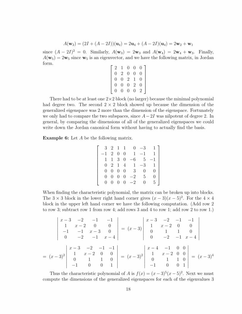
since (A − 2I)2 = 0. Similarly, A(w3) = 2w3 and A(w4) = 2w4 + w3. Finally,A(w5) = 2w5 since w5 is an eigenvector, and we have the following matrix, in Jordanform.

2 1 0 0 00 2 0 0 00 0 2 1 00 0 0 2 00 0 0 0 2

There had to be at least one 2×2 block (no larger) because the minimal polynomial

had degree two. The second 2 × 2 block showed up because the dimension of thegeneralized eigenspace was 2 more than the dimension of the eigenspace. Fortunatelywe only had to compare the two subspaces, since A−2I was nilpotent of degree 2. Ingeneral, by comparing the dimensions of all of the generalized eigenspaces we couldwrite down the Jordan canonical form without having to actually find the basis.

Example 6: Let A be the following matrix.

3 2 1 1 0 −3 1−1 2 0 0 1 −1 1

1 1 3 0 −6 5 −10 2 1 4 1 −3 10 0 0 0 3 0 00 0 0 0 −2 5 00 0 0 0 −2 0 5

When finding the characteristic polynomial, the matrix can be broken up into blocks.The 3 × 3 block in the lower right hand corner gives (x − 3)(x − 5)2. For the 4 × 4block in the upper left hand corner we have the following computation. (Add row 2to row 3; subtract row 1 from row 4; add rows 3 and 4 to row 1; add row 2 to row 1.)∣∣∣∣∣∣∣∣

x− 3 −2 −1 −11 x− 2 0 0−1 −1 x− 3 00 −2 −1 x− 4

∣∣∣∣∣∣∣∣ = (x− 3)

∣∣∣∣∣∣∣∣x− 3 −2 −1 −1

1 x− 2 0 00 1 1 00 −2 −1 x− 4

∣∣∣∣∣∣∣∣= (x− 3)2

∣∣∣∣∣∣∣∣x− 3 −2 −1 −1

1 x− 2 0 00 1 1 0−1 0 0 1

∣∣∣∣∣∣∣∣ = (x− 3)2

∣∣∣∣∣∣∣∣x− 4 −1 0 0

1 x− 2 0 00 1 1 0−1 0 0 1

∣∣∣∣∣∣∣∣ = (x− 3)4

Thus the characteristic polynomial of A is f(x) = (x− 3)5(x− 5)2. Next we mustcompute the dimensions of the generalized eigenspaces for each of the eigenvalues 3

18

and 5. We first row-reduce A− 3I.

A− 3I =

0 2 1 1 0 −3 1−1 −1 0 0 1 −1 1

1 1 0 0 −6 5 −10 2 1 1 1 −3 10 0 0 0 0 0 00 0 0 0 −2 2 00 0 0 0 −2 0 5

1 1 0 0 0 0 00 2 1 1 0 0 00 0 0 0 1 0 00 0 0 0 0 1 00 0 0 0 0 0 10 0 0 0 0 0 00 0 0 0 0 0 0

We conclude that the eigenspace corresponding to 3 has dimension 7 − 5 = 2. Nextwe compute (A− 3I)2 and row-reduce it.

(A− 3I)2 =

−1 1 1 1 1 −6 41 −1 −1 −1 −1 2 0

−1 1 1 1 −7 6 0−1 1 1 1 1 −6 4

0 0 0 0 0 0 00 0 0 0 −4 4 00 0 0 0 −4 0 4

1 −1 −1 −1 0 1 00 0 0 0 1 −1 00 0 0 0 0 1 −10 0 0 0 0 0 00 0 0 0 0 0 00 0 0 0 0 0 00 0 0 0 0 0 0

Thus the generalized eigenspace of degree 2 of the eigenvalue 3 has dimension 7−3 = 4.The dimension of the generalized eigenspace of degree 3 can be at most 5, since(x− 3) has exponent 5 in the characteristic polynomial, and so it must be equal to 5.Nonetheless, we can easily do the computation which shows that (A− 3I)3 has rank2, and hence a nullity of 5.

(A− 3I)3 =

0 0 0 0 0 −8 80 0 0 0 0 0 00 0 0 0 −16 16 00 0 0 0 0 −8 80 0 0 0 0 0 00 0 0 0 −8 8 00 0 0 0 −8 0 8

To summarize, we can find two linearly independent eigenvectors, two linearly inde-pendent generalized eigenvectors of rank 2, and one linearly independent generalizedeigenvector of rank 3. In the matrix for A, the primary block corresponding to theeigenvalue 3 will have one secondary 3 × 3 block, corresponding to the one general-ized eigenvector of rank 3. Since there are two generalized eigenvectors of rank 2, onewill go in the 3 × 3 block, and one will go into the next secondary block, which willtherefore be 2× 2.

Finally, we must compute the dimensions of the generalized eigenspaces for 5.Since the exponent of (x− 5) in the characteristic polynomial is 2, the dimension will

19

be 2 and we should reach this in either one step or two. In fact, by looking at thelast three rows we can tell that the rank is no more than 5, so the nullity must be 2,giving 2 eigenvectors.

A− 5I =

−2 2 1 1 0 −3 1−1 −3 0 0 1 −1 1

1 1 −2 0 −6 5 −10 2 1 −1 1 −3 10 0 0 0 −2 0 00 0 0 0 −2 0 00 0 0 0 −2 0 0

We can now give the Jordan canonical form of the matrix A.

3 1 0 0 0 0 00 3 1 0 0 0 00 0 3 0 0 0 00 0 0 3 1 0 00 0 0 0 3 0 00 0 0 0 0 5 00 0 0 0 0 0 5

Example 7: Suppose that A is a matrix with characteristic polynomial f(x) =(x − 7)6 and minimal polynomial p(x) = (x − 7)3. Then A must be a 6 × 6 matrix,and the first secondary block must be a 3 × 3 block since the minimal polynomialhas degree 3. We do not have enough information to determine A, but we have listedbelow all possible cases.

7 1 00 7 10 0 7

7 1 00 7 10 0 7

7 1 00 7 10 0 7

7 10 7

7

7 1 00 7 10 0 7

77

7

Proposition: Let A and B be n× n matrices over the field C of complex numbers.Then A and B are similar if and only if they have the same Jordan canonical form,up to the order of the eigenvalues.Proof. The assumption that the matrices have complex entries guarantees that theircharacteristic polynomials can be factored completely, and so they can be put intoJordan canonical form.

If A and B are similar, then they represent the same linear transformation T .The Jordan canonical form depends only on the linear transformation T , since it is

20

constructed from the zeros of the characteristic polynomial of T and the dimensionsof the corresponding generalized eigenspaces. However, we have no way to specifythe order of the eigenvalues. Thus A and B have the same Jordan canonical form,except for the order of the eigenvalues.

Conversely, if A and B have the same Jordan canonical form, except for the orderof the eigenvalues, then the matrices in Jordan canonical form are easily seen to besimilar. Thus A and B are similar to the similar matrices. Since similarity is anequivalence relation, it follows that A and B are similar. �

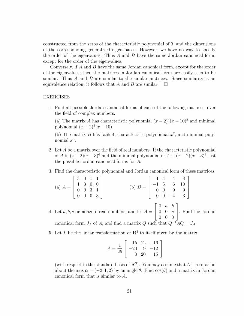
EXERCISES

1. Find all possible Jordan canonical forms of each of the following matrices, overthe field of complex numbers.

(a) The matrix A has characteristic polynomial (x− 2)4(x− 10)3 and minimalpolynomial (x− 2)3(x− 10).

(b) The matrix B has rank 4, characteristic polynomial x7, and minimal poly-nomial x3.

2. Let A be a matrix over the field of real numbers. If the characteristic polynomialof A is (x− 2)(x− 3)6 and the minimal polynomial of A is (x− 2)(x− 3)3, listthe possible Jordan canonical forms for A.

3. Find the characteristic polynomial and Jordan canonical form of these matrices.

(a) A =

3 0 1 11 3 0 00 0 3 10 0 0 3

(b) B =

1 4 4 8

−1 5 6 100 0 9 90 0 −4 −3

4. Let a, b, c be nonzero real numbers, and let A =

0 a b0 0 c0 0 0

. Find the Jordan

canonical form JA of A, and find a matrix Q such that Q−1AQ = JA.

5. Let L be the linear transformation of R3 to itself given by the matrix

A =1

25

15 12 −16−20 9 −12

0 20 15

(with respect to the standard basis of R3). You may assume that L is a rotationabout the axis a = (−2, 1, 2) by an angle θ. Find cos(θ) and a matrix in Jordancanonical form that is similar to A.

21