Normative evidence accumulation in unpredictable …Gold,Kable_2015.pdf · Normative evidence...
27
elifesciences.org RESEARCH ARTICLE Normative evidence accumulation in unpredictable environments Christopher M Glaze 1,2 *, Joseph W Kable 2 , Joshua I Gold 1 1 Department of Neuroscience, University of Pennsylvania, Philadelphia, United States; 2 Department of Psychology, University of Pennsylvania, Philadelphia, United States Abstract In our dynamic world, decisions about noisy stimuli can require temporal accumulation of evidence to identify steady signals, differentiation to detect unpredictable changes in those signals, or both. Normative models can account for learning in these environments but have not yet been applied to faster decision processes. We present a novel, normative formulation of adaptive learning models that forms decisions by acting as a leaky accumulator with non-absorbing bounds. These dynamics, derived for both discrete and continuous cases, depend on the expected rate of change of the statistics of the evidence and balance signal identification and change detection. We found that, for two different tasks, human subjects learned these expectations, albeit imperfectly, then used them to make decisions in accordance with the normative model. The results represent a unified, empirically supported account of decision-making in unpredictable environments that provides new insights into the expectation-driven dynamics of the underlying neural signals. DOI: 10.7554/eLife.08825.001 Introduction Even the simplest perceptual judgments, like detecting the presence of a dim light, take time for the brain to process (Luce, 1986). Some of this time reflects sensory and motor processing, but a considerable fraction is dedicated to the decision process that converts the incoming sensory information into a categorical judgment that guides behavior (Sternberg, 2001). Under certain conditions, this temporally unfolding process serves a normative purpose: improving the accuracy of the decision by reducing uncertainty about the source or identity of noisy inputs. The sequential probability ratio test (SPRT), drift-diffusion model, and related sequential-sampling models are forms of ‘belief-updating’ rules for this normative process, based on perfect integration over time of the logarithm of the likelihood ratio (LLR) associated with each data point (Barnard, 1946; Wald, 1947; Good, 1979; Link, 1992; Gold and Shadlen, 2001; Smith and Ratcliff, 2004; Bogacz et al., 2006). These models have been useful for studying neural mechanisms of decision-making (Gold and Shadlen, 2007) but are normative for only a restricted set of conditions in which: (1) the ideal starting time-point for accumulation is known (e.g., given by the onset of an experimental trial); and (2) the statistics of the incoming information are perfectly stable throughout the entire sequence, with no change in the underlying signal and all noise coming from the same probability distribution. Perfect integration can be particularly problematic for tasks that require the detection of signal changes (Clifford and Ibbotson, 2002). When there is certainty about when the change might occur, integrated signals from before vs after that time can be compared to detect the change (Green and Swets, 1966; Macmillan and Creelman, 2004). However, when there is temporal uncertainty about the change, integrating evidence at the wrong time might miss the signal or add unnecessary noise, resulting in a loss of sensitivity to the change (Lasley and Cohn, 1981). Several possible solutions to this problem have been proposed, including using a leaky integrator, taking a time derivative of the evidence to identify changes, or using knowledge of the spatial and temporal structure of the stimulus to guide a more directed search for the evidence *For correspondence: cglaze@ sas.upenn.edu Competing interests: The authors declare that no competing interests exist. Funding: See page 25 Received: 19 May 2015 Accepted: 30 August 2015 Published: 31 August 2015 Reviewing editor: Timothy Behrens, Oxford University, United Kingdom Copyright Glaze et al. This article is distributed under the terms of the Creative Commons Attribution License, which permits unrestricted use and redistribution provided that the original author and source are credited. Glaze et al. eLife 2015;4:e08825. DOI: 10.7554/eLife.08825 1 of 27
-
Upload
hoangkhuong -
Category
Documents
-
view
216 -
download
0
Transcript of Normative evidence accumulation in unpredictable …Gold,Kable_2015.pdf · Normative evidence...

elifesciences.org
RESEARCH ARTICLE
Normative evidence accumulation inunpredictable environmentsChristopher M Glaze1,2*, Joseph W Kable2, Joshua I Gold1
1Department of Neuroscience, University of Pennsylvania, Philadelphia, United States;2Department of Psychology, University of Pennsylvania, Philadelphia, United States
Abstract In our dynamic world, decisions about noisy stimuli can require temporal accumulation
of evidence to identify steady signals, differentiation to detect unpredictable changes in those
signals, or both. Normative models can account for learning in these environments but have not yet
been applied to faster decision processes. We present a novel, normative formulation of adaptive
learning models that forms decisions by acting as a leaky accumulator with non-absorbing bounds.
These dynamics, derived for both discrete and continuous cases, depend on the expected rate of
change of the statistics of the evidence and balance signal identification and change detection.
We found that, for two different tasks, human subjects learned these expectations, albeit
imperfectly, then used them to make decisions in accordance with the normative model. The results
represent a unified, empirically supported account of decision-making in unpredictable environments
that provides new insights into the expectation-driven dynamics of the underlying neural signals.
DOI: 10.7554/eLife.08825.001
IntroductionEven the simplest perceptual judgments, like detecting the presence of a dim light, take time for
the brain to process (Luce, 1986). Some of this time reflects sensory and motor processing, but
a considerable fraction is dedicated to the decision process that converts the incoming sensory
information into a categorical judgment that guides behavior (Sternberg, 2001). Under certain
conditions, this temporally unfolding process serves a normative purpose: improving the accuracy
of the decision by reducing uncertainty about the source or identity of noisy inputs. The sequential
probability ratio test (SPRT), drift-diffusion model, and related sequential-sampling models are
forms of ‘belief-updating’ rules for this normative process, based on perfect integration over time
of the logarithm of the likelihood ratio (LLR) associated with each data point (Barnard, 1946;
Wald, 1947; Good, 1979; Link, 1992; Gold and Shadlen, 2001; Smith and Ratcliff, 2004; Bogacz
et al., 2006). These models have been useful for studying neural mechanisms of decision-making
(Gold and Shadlen, 2007) but are normative for only a restricted set of conditions in which: (1) the ideal
starting time-point for accumulation is known (e.g., given by the onset of an experimental trial); and
(2) the statistics of the incoming information are perfectly stable throughout the entire sequence, with
no change in the underlying signal and all noise coming from the same probability distribution.
Perfect integration can be particularly problematic for tasks that require the detection of signal
changes (Clifford and Ibbotson, 2002). When there is certainty about when the change might
occur, integrated signals from before vs after that time can be compared to detect the change
(Green and Swets, 1966; Macmillan and Creelman, 2004). However, when there is temporal
uncertainty about the change, integrating evidence at the wrong time might miss the signal or
add unnecessary noise, resulting in a loss of sensitivity to the change (Lasley and Cohn, 1981).
Several possible solutions to this problem have been proposed, including using a leaky integrator,
taking a time derivative of the evidence to identify changes, or using knowledge of the spatial
and temporal structure of the stimulus to guide a more directed search for the evidence
*For correspondence: cglaze@
sas.upenn.edu
Competing interests: The
authors declare that no
competing interests exist.
Funding: See page 25
Received: 19 May 2015
Accepted: 30 August 2015
Published: 31 August 2015
Reviewing editor: Timothy
Behrens, Oxford University,
United Kingdom
Copyright Glaze et al. This
article is distributed under the
terms of the Creative Commons
Attribution License, which
permits unrestricted use and
redistribution provided that the
original author and source are
credited.
Glaze et al. eLife 2015;4:e08825. DOI: 10.7554/eLife.08825 1 of 27

(Henning et al., 1975; Nachmias and Rogowitz, 1983; Smith, 1995, 1998; Verghese et al., 1999;
Schrater et al., 2000). However, none of these solutions provide more general insights into how to
balance the operations used to identify both steady, noisy, signals and unpredictable changes in
those signals.
Here we present a normative model of decisions between two alternatives that provides such an
account. In a variety of learning and other tasks, the tradeoff between signal identification and change
detection has been related to inference algorithms in hidden Markov models and other Bayesian
algorithms. These algorithms estimate statistical parameters in the presence of abrupt and unpredict-
able change-points in the otherwise stable statistics of a data-generating process (Zakai, 1965; Liptser
and Shiryaev, 1977; Rabiner, 1989; Yu and Dayan, 2005; Adams and MacKay, 2007; Behrens et al.,
2007; Fearnhead and Liu, 2007; Wilson et al., 2010; McGuire et al., 2014; Sato and Kording, 2014).
Here we express these algorithms in a novel form that, unlike previous change-point models, is based
on the LLR and thus can be compared directly to standard decision models based on evidence
accumulation (Gold and Shadlen, 2001; Usher and McClelland, 2001; Smith and Ratcliff, 2004;
Bogacz et al., 2006). The form thus yields quantitative predictions of both choice behavior and the
underlying neural signals for decisions about unstable, noisy stimuli (Gold and Shadlen, 2007). A key
feature of the model is that the expected amount of instability in the environment governs the temporal
dynamics of the decision process. When perfect stability is expected, evidence is accumulated perfectly.
Otherwise, evidence is accumulated with a leak (Usher and McClelland, 2001) to a non-absorbing
boundary that expedites the identification of unexpected changes that should re-start the accumulation
process, where both the leak and the boundary depend on the level of expected instability in the
environment. These expectation-dependent dynamics represent a novel view of leaky, saturating, or
otherwise imperfect evidence accumulation, which here may be understood as facilitating, rather than
eLife digest Organisms gather information from their surroundings to make decisions.
Traditionally, neuroscientists have investigated decision-making by first asking what would be
optimal for the animal, and then seeing whether and how the brain implements the optimal process.
This approach has assumed that the environment consists of noisy, but stable, signals that the brain
must decipher by accumulating information over time and ‘averaging out’ the noise.
Previous research had suggested that most animals can accumulate information. However, these
studies also showed that animals, including humans, often fall short of the optimal solution by being
overly sensitive to noise and failing to completely average it out. Of course, in real life, the signals
themselves can change abruptly and unpredictably, challenging us to distinguish noise from changes
in the underlying signals. If a moving target suddenly jolts to the right, is that change part of the
normal jitter that should be ignored, or does it predict where the target will be next? How do we
know when to keep old information that is still relevant to the decision, and when to discard the old
information because a change might have occurred that renders it irrelevant?
Glaze et al. have addressed this question by building optimal change detection into the traditional
‘information-accumulation’ framework. The model suggests that what researchers previously
thought was an over-sensitivity to noise might actually be optimal for the real-life challenge of
detecting change. In two different tasks, Glaze et al. tested human volunteers to see if they could
make decisions in ways predicted by the model. One task involved the volunteers making decisions
about which one of two possible sources of noisy signals generated a given piece of information, with
the correct answer changing unpredictably every 1–20 trials. The other task involved looking at
a crowd of moving dots, which jolted and wobbled as they changed direction, and the volunteers had
to decide which direction the dots were moving at the end of each trial.
Both experiments showed that the volunteers were remarkably good at making decisions in the
ways predicted by the new model, and incorporated learned expectations about the rate of change
in underlying signals. The results suggest that humans, and potentially other organisms, are capable
of detecting changes in the optimal ways suggested by the decision-making model. The study also
makes predictions about what kinds of neural patterns neuroscientists might find when measuring
brain activity while organisms do similar tasks.
DOI: 10.7554/eLife.08825.002
Glaze et al. eLife 2015;4:e08825. DOI: 10.7554/eLife.08825 2 of 27
Research article Neuroscience

hindering, statistical inference. We show that human decision-makers can use these dynamics to
solve two different tasks on different timescales (tens of seconds vs hundreds of milliseconds) that
each requires information accumulation in the presence of unpredictable change-points occurring at
different rates.
Results
ModelConsider a decision about which of two alternatives is the present source of a sequence of noisy data
arriving over time. We derived a belief-update rule for these kinds of decisions based on Bayesian
principles that have typically been used to understand learning processes in dynamic environments on
relatively slow timescales (Figure 1A) (Yu and Dayan, 2005; Adams andMacKay, 2007; Behrens et al.,
2007; Fearnhead and Liu, 2007; Wilson et al., 2010; McGuire et al., 2014; Sato and Kording, 2014).
This rule both accounts for environmental instability and relates directly to models of perfect, leaky, and
bounded accumulation that have been used to understand decision processes in stable environments
(Link, 1992; Gold and Shadlen, 2001; Usher and McClelland, 2001; Smith and Ratcliff, 2004; Bogacz
et al., 2006). We define belief as the logarithm of the posterior odds of the alternative sources of
information (L) given all information collected until a given time point. The sign of L indicates which
source is currently believed to be generating the information, and the magnitude of L indicates how
certain that belief is. The update rule is optimal when there is a fixed probability that the source could
switch to the alternative at any time (i.e., according to a Bernoulli process). Specifically,
Ln =ψðLn−1;HÞ+ LLRn; (1)
where Ln is the belief at time step n, LLRn is the sensory evidence (the log likelihood ratio) at step n, H
(the ‘hazard rate’) is the expected probability at each time step that the source will switch from one
alternative to the other, and ψ is the time-varying prior expectation (the logarithm of the prior odds)
about the source before observing the new evidence:
ψðLn−1;HÞ= Ln−1 + log
�1−H
H+ expð−Ln−1Þ
�− log
�1−H
H+ expðLn−1Þ
�: (2)
The prior expectation ψ is the key feature of the model, balancing integration to identify steady
signals and differentiation to detect changes by dynamically filtering sensory information in a way
that depends on both L and H (Figures 1, 2). For the special case of H = 0 (perfect stability), the
two rightmost terms in Equation 2 cancel. In this case, the update Equation 1 reduces to perfect
accumulation as in random-walk and related decision models used to identify steady, but noisy,
signals (Figure 1D) (Smith and Ratcliff, 2004; Bogacz et al., 2006). In contrast, when H is high
and changes are expected, accumulation over time is severely limited to facilitate change detection
(Figures 1F, 2G). For intermediate values of H, these operations trade-off to emphasize change
detection at the expense of steady signal identification (for higher H) or vice versa (for lower H;
Figures 1E, 2G). Finally, in the special case of H = 0.5, the history of evidence is irrelevant at all
times and all three terms in Equation 2 cancel, so ψ = 0 and Ln = LLRn.
To gain further insight into the dynamics of the model and how it controls this trade-off, we made
approximations of the nonlinearity in Equation 2:
ψðLn−1;HÞ≈ ð1−KnÞ× Ln−1 + θn; (3)
≈ ð1− 2HÞ× Ln−1 when Ln−1 ≈ 0; (3a)
≈ log½ð1−HÞ=H�when Ln−1≫0; (3b)
≈−log½ð1−HÞ=H� when Ln−1≪0: (3c)
Here Kn governs the leakiness of the accumulation process, and θn, governs a bias. Both
parameters are adaptive, depending on both H and Ln, with dynamics that jointly establish a boundary
on the prior and thus limit subsequent belief strength. The dynamics include two regimes, as follows.
Glaze et al. eLife 2015;4:e08825. DOI: 10.7554/eLife.08825 3 of 27
Research article Neuroscience

First, when beliefs are uncertain (i.e., regimes around Ln − 1 = 0 in Figures 1B, 2A,C; Equation 3a, in
which Kn predominates over θn), the model acts like a leaky accumulator, in which the prior expectation
is a fraction of the previous belief (Busemeyer and Townsend, 1993; Usher and McClelland, 2001;
Bogacz et al., 2006; Tsetsos et al., 2012). Thus, the dynamics of a leaky accumulator can, in principle,
act like the normative model, but only in the low-certainty regime (Figure 3). In this regime, the
normative leak is adaptive, which has been demonstrated previously (Ossmy et al., 2013), and is
directly dependent on H, which has not been described previously. For low H and thus relative stability,
a small leak provides long integration times. For H ≈ 0.5 (the correct answer is equally likely to stay or
Figure 1. Normative model. (A) Illustration of the belief-updating process. (B) Discrete-time log-prior odds at
a given moment as a function of the belief at the prior moment, plotted as Equation 2 for different values of H.
(C) Continuous-time version of the model, with log-prior odds plotted as a function of belief, computed by
numerically integrating Equation 4 with dx(t) = 0 over a 16 ms interval. Here expected instability (λ) has units of
number of changes per s. Thus, λ → ∞ is analogous to discrete-time H → 0.5. (D–F) Examples of how the normative
model (solid lines) and perfect accumulation (dashed gray lines) process a time-dependent stimulus (light vs dark
grey for the two alternatives, shown at the top) for different hazard rates (H).
DOI: 10.7554/eLife.08825.003
The following figure supplement is available for figure 1:
Figure supplement 1. Dynamics of the continuous-time model.
DOI: 10.7554/eLife.08825.004
Glaze et al. eLife 2015;4:e08825. DOI: 10.7554/eLife.08825 4 of 27
Research article Neuroscience
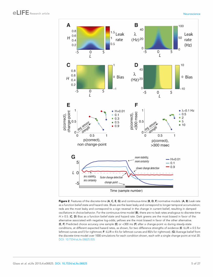
Figure 2. Features of the discrete-time (A, C, E, G) and continuous-time (B, D, F) normative models. (A, B) Leak rate
as a function belief state and hazard rate. Blues are the least leaky and correspond to longer temporal accumulation;
reds are the most leaky and correspond to a sign reversal in the change in current belief, resulting in damped
oscillations in choice behavior. For the continuous-time model (B), there are no leak rates analogous to discrete-time
H > 0.5. (C, D) Bias as a function belief state and hazard rate. Dark greens are the most biased in favor of the
alternative associated with negative log-odds; yellows are the most biased in favor of the other alternative.
(E, F) Predicted choice accuracy one sample (E) or <300 ms (F) after a change-point vs during steady-state
conditions, at different expected hazard rates, as shown, for two difference strengths of evidence (E: |LLR| = 0.5 for
leftmost curves and 5 for rightmost; F: |LLR| = 4/s for leftmost curves and 80/s for rightmost). (G) Average belief from
the discrete-time model over 1000 simulations for each condition shown, each with a single change-point at trial 20.
DOI: 10.7554/eLife.08825.005
Glaze et al. eLife 2015;4:e08825. DOI: 10.7554/eLife.08825 5 of 27
Research article Neuroscience
switch after each sample), the model discards all historical information and L depends only on LLR.
For H > 0.5 (the correct answer is more likely to switch after each sample), the prior expectation
undergoes damped oscillations (Figure 2G), even when the source of evidence is transiently stable.
These oscillations repeatedly switch the direction of existing beliefs because of the high expected
probability of change on each discrete time step.
Second, as the magnitude of Ln − 1 increases and belief certainty becomes high (i.e., regimes
around Ln − 1 far from zero in Figures 1B, 2A,C; Equation 3b,c, in which θn predominates over Kn),
such as when the incoming evidence is strong or during periods of stability in the source, the prior
expectation approaches a ‘stabilizing boundary’ whose height directly depends on H. Thus, the
dynamics of a model that stabilizes the decision process at a hazard-dependent value can, in principle,
act like the normative model, but only in the high-certainty regime (Figure 3). This boundary represents
a suspension of the accumulation process but, unlike the decision bound in the SPRT and related
models (Barnard, 1946;Wald, 1947;Good, 1979; Link, 1992; Smith and Ratcliff, 2004; Bogacz et al.,
2006; Gold and Shadlen, 2007), does not terminate the decision process. Instead, it stabilizes Ln when
no changes occur (i.e., temporarily ending further evidence accumulation) while still allowing for the
sampling of new evidence that might lead to changes in belief and a re-start of the accumulation
process (Resulaj et al., 2009). The stabilizing boundary is also in contrast to the asymptote in leaky
accumulation, which increases linearly with the strength of evidence (Busemeyer and Townsend, 1993;
Usher and McClelland, 2001; Bogacz et al., 2006; Tsetsos et al., 2012).
Together these properties navigate an inherent trade-off between identification of steady
signals and change detection. This trade-off depends on both evidence strength and expected H
(Figure 2E,G). For weak evidence, the trade-off is most severe, as the model uses expected H to
err on the side of either detecting changes quickly when H is high or identifying stable signals
when H is low. As the strength of evidence increases, performance improves steadily for both conditions
and the trade-off diminishes.
Continuous-time versionWe also developed a continuous-time version of the model (Figure 1C) that allowed for a more direct
comparison to drift-diffusion and other continuous-time models of decision-making (Figure 1C)
(Smith and Ratcliff, 2004; Bogacz et al., 2006; Gold and Shadlen, 2007). The model is based on the
optimal filter for a Markov jump process with two states and stationary white-noise emissions (Zakai,
1965; Liptser and Shiryaev, 1977; Crisan and Rozovskii, 2011). Here we write the incoming evidence
as a continuous-time sequence of noisy observations: dx(t) = h(t)d(t) + σdW, where h(t) = ±μ, with the
sign depending on which source is generating data at time t, and σ is the standard deviation of the noise
in a standard Wiener process dW. The source h(t) jumps between states at an average rate λ, with jumps
occurring as a Poisson process. Letting A = 2μ/σ2:
dLðtÞ=−2λsinhLðtÞdt +AdxðtÞ: (4)
The result can be viewed as a nonlinear filter for the incoming evidence that is more general than
the perfect or leaky integration central to previous models of decision-making between two
alternatives (Busemeyer and Townsend, 1993; Usher and McClelland, 2001; Bogacz et al., 2006).
In the special case that λ = 0, dL(t) = Adx(t), which is perfect integration of the noisy observations dx(t).
Approximations of this model are similar to those for the discrete-time model (Figure 2B,D).
When beliefs are uncertain (L ≈ 0), dL ≈ −2λLdt + Adx(t), which results in an Ornstein-Uhlenbeck
process over periods in which the source is perfectly stable (Busemeyer and Townsend, 1993;
Bogacz et al., 2006). As certainty increases (|L| > 0), a simultaneous increase in leak rate and bias
drives the decision variable to a stabilizing boundary (Figure 1C) with a probability distribution
that has a heavy tail, reflecting dynamics that facilitate the detection of subsequent changes
(Figure 1—figure supplement 1). As with the discrete-time model, these dynamics navigate the
trade-off between identification of steady signals and change detection in a way that depends
on both evidence strength and expected λ (Figure 2F).
PsychophysicsWe used two separate tasks to investigate if and how human subjects could use these dynamics to
adapt to different rates of change and find the optimal trade-off between stable signal identification
and change detection. For both tasks, we found that: (1) subjects adapted, albeit imperfectly, to
Glaze et al. eLife 2015;4:e08825. DOI: 10.7554/eLife.08825 6 of 27
Research article Neuroscience

different hazard rates (via comparisons to a suboptimal model, which ignored block-wise
changes in H) and used their subjective estimates of hazard rate in a manner consistent with the
normative model; and (2) their choice dynamics were better described by the normative model than two
other adaptive, but suboptimal, alternatives inspired by the approximations to the normative model
(one was an accumulator with a leak that could vary as a free parameter for each hazard-specific
block of trials but no stabilizing boundary; the other was a perfect accumulator with a stabilizing
boundary that could vary as a free parameter for each hazard-specific block of trials; see Figure 3).
‘Triangles’ taskThis task required subjects to make trial-by-trial choices about which of two spatially separated
triangles on a computer screen was the source of a single data point presented on that trial,
represented as the position of a star on the screen (Figure 4A,B). Subjects could thus make choices
based on accumulated evidence after each new sample of data, with the LLR for each star
corresponding to its position relative to each triangle. The correct source changed at a hazard rate
that was constant within a block of trials but varied across blocks (0.05–0.95). In a subset of sessions
(65 of 111), learning was facilitated by beginning and ending each block of trials with stretches of trial-
by-trial feedback about the correct answer. However, subjects were never instructed on what the
hazard rates were or when they would change.
The subjects were able to adapt their decision-making to these different hazard rates, as assessed
by direct fits of their choice data by the normative model. Specifically, models that allowed
subjective H to freely vary by block provided better fits to the data than a suboptimal model that
ignored the block-wise changes in objective H (median ± bootstrapped SEM difference of Bayesian
Information Criterion, or BIC, from normative vs block-independent H fits was −23.721 ± 9.671,
Wilcoxon signed-rank test, p < 0.0001; per subject, the normative fits were better in 43 of 48 subjects
using a signed-rank test, Bonferroni corrected p < 0.05). Overall, the normative model performed well,
with choice residuals centered around zero (mean ± std deviance residual = 0.003 ± 0.458) and
Figure 3. Two ways of approximating the discrete-time normative model, accounting separately for its dynamics
when the sensory evidence is consistently weak (A, average |LLR| ≈ 0.25) or strong (B, average |LLR| ≈ 10). As in Figure
1B, each panel has discrete-time log-prior odds as a function of the belief at the previous moment. Dark blue
lines correspond to the normative model for H = 0.1. Light blue lines correspond to a leaky accumulator with no
bias, related to the linear approximation in Equation 3a but optimized to best approximate the normative model
separately for each average evidence strength in A and B. Magenta lines correspond to perfect accumulation (no leak)
to a stabilizing boundary related to Equation 3b,c, also optimized for each evidence strength. In general, the leaky
accumulator is better at approximating the normative solution for weak sensory evidence (A), whereas the bounded
accumulator is better at approximating the solution for strong sensory evidence (B).
DOI: 10.7554/eLife.08825.006
Glaze et al. eLife 2015;4:e08825. DOI: 10.7554/eLife.08825 7 of 27
Research article Neuroscience

a reasonably close match to the choice data (median ± bootstrapped SEM McFadden’s r2 of 0.895 ±0.016 across subjects). Moreover, the estimated values of subjective H from these fits were strongly
correlated with objective H across all subjects (Pearson’s r = 0.721, p < 0.0001; Figure 4C), with 47 of 48
individual subjects showing a regression slope of subjective on objective H that was >0 and in 46 of
those cases was also <1 (Figure 4D, median ± bootstrapped SEM regression slope = 0.402 ±0.042). However, although the subjects adapted their decision-making behavior appropriately
for different values of H, their subjective estimates of H tended towards H ∼ 0.5, for which the
history of evidence is irrelevant. This tendency to mis-estimate extreme hazard rates did not appear to
reflect insufficient learning opportunities, because these trends persisted even when restricting
fits to the last 200 trials of each block (across subjects and blocks, bootstrapped regression
slope of subjective on objective H = 0.373 ± 0.044; see also Figure 4—figure supplement 1) or
to blocks beginning with explicit, trial-to-trial feedback (regression slope = 0.562 ± 0.038).
The subjects appeared to be using these learned, subjective estimates of hazard rate in a manner
consistent with the normative model, for several reasons. First, their choice dynamics directly
reflected biases predicted by the two regimes of the normative model (Equation 3, Figure 5A–F).
When certainty was high (i.e., choices just following a trial in which the star position was far to the left
or right), the subjects consistently showed hazard-dependent biases that were predicted by the
stabilizing boundary of the model: weak evidence interpreted as stability for low H and change for
high H (Spearman’s r = 0.890, p < 0.0001, comparing predicted and actual biases from individual
Figure 4. Triangles task and normative model fits. (A) Example task screen. Triangles and surrounding greenish
clouds represent the means and variances of the two generative processes; red star is a single sample (in this case
generated by the left process). (B) Sample trials, with actual star position indicated by blue circles and subject
choices indicated by red ‘x’. Star positions close to the center represent weak evidence for either of the alternatives
because the respective probabilities of either source generating the star position are close. Star positions towards
the edge of the screen represent strong evidence for the triangle to which the star is closest. (C) Block-wise
subjective (fit) H vs objective H. Dotted line is unity; solid line is a least-squares fit. (D) Histogram of slope coefficients
from least-squares fits as in C, calculated for individual subjects.
DOI: 10.7554/eLife.08825.007
The following figure supplement is available for figure 4:
Figure supplement 1. Two examples of subjects adapting to objective hazard rate across an entire experimental
session.
DOI: 10.7554/eLife.08825.008
Glaze et al. eLife 2015;4:e08825. DOI: 10.7554/eLife.08825 8 of 27
Research article Neuroscience

blocks; Figure 5A,B). When weak evidence persisted without change-points for a run of trials following
a change-point, choice dynamics consistently reflected the hazard-dependent leak predicted by
the model (Figure 2G, Figure 5D,E): gradual updates for low subjective H, immediate updates for
subjective H ≈ 0.5, and damped oscillations for high subjective H (including lower accuracy on two
vs one trial following the change-point). Fits to the block-independent model did not show these
H-dependent choice dynamics, confirming that the choice dynamics did not result from any
differences in how the randomly generated stars were sampled under the different conditions
used for these analyses (Figure 5C,F).
Second, the subjects’ decision processes reflected a strong, hazard- and evidence-strength-
dependent trade-off between detecting changes and identifying steady signals, as predicted by the
normative model (Figure 5G–L). When the evidence was weak (star positions close to the midline),
accuracy following a change-point was highest for high H (mean ± bootstrapped SEM across blocks =73.7 ± 2.4% correct) then declined steadily for intermediate (66.4 ± 1.2%) and low H (50.0 ± 7.3%;
Spearman’s correlation between change-point accuracy and H was 0.559, p < 0.0001, vs a predicted
correlation from the normative model of 0.651). In contrast, accuracy on non change-point trials with the
same strength of evidence was lowest for high H (57.1 ± 4.1%) then improved steadily for
intermediate (71.4 ± 1.2%) and low H (81.1 ± 2.2%; Spearman’s correlation between non change-
point accuracy and H was −0.502, p < 0.0001, vs a normative prediction of −0.625; Figure 5G,H).
When the evidence was strong, the trade-off was much smaller, as predicted by the normative model
(Spearman’s correlation between change-point accuracy and H was −0.040, p = 0.557 and between non
change-point accuracy and H was −0.005, p = 0.945; normative predictions were 0.027 and 0.010,
respectively; Figure 5J,K). Fits to the block-independent model did not show these H-dependent trade-
offs, for either weak or strong evidence (Figure 5I,L).
Third, we used choice data to directly estimate the mapping of subjective beliefs to priors (Ln − 1 to Ψn,
Figure 6; compare to Figure 1B). Like for the normative model, the estimated mappings depended
on subjective H (one-way MANOVA for the groups shown in Figure 6A, p < 0.0001). Moreover, for
Figure 5. Triangles task choice data pooled across all 48 subjects (top row), plus predictions from fits to the
normative model allowing a different subjective hazard rate to be assigned to each block (middle row) and from fits
to a model with subjective hazard rates randomly assigned across trials (bottom row). Colors are different ranges
of objective H, as shown in panel D. Errorbars are bootstrapped sem. (A–C) Probability of switching choices as
a function of the LLR for a change in the correct answer. Data were restricted to trials following strong evidence
(|LLR| > 4) to directly investigate the ‘strong belief’ regime of the model predictions. (D–F) Probability of switching
sides in which a strong LLR (|LLR| > 4) for the original side was followed by a change-point and weak (|LLR| < 2)
evidence for the opposite side. Significant differences by H in subject data are indicated by asterisks (Bonferroni
corrected p < 0.05, χ2 test). (G–L) Block-by-block choice accuracy on change-point vs non-change-point trials when
the evidence (magnitude of LLR, as indicated) was relatively weak (G–I) or strong (J–L). Points are individual blocks
that included ≥5 trials with the indicated conditions.
DOI: 10.7554/eLife.08825.009
Glaze et al. eLife 2015;4:e08825. DOI: 10.7554/eLife.08825 9 of 27
Research article Neuroscience

each H-group, these mappings matched predictions of the normative model (Figure 6B,E;
Hotelling’s t-test comparing data and model, p = 0.189, 0.321, and 0.086 for low, medium, and high
values of objective H, respectively).
In contrast, the choice data from the triangles task were not as well matched by either of the two
adaptive, suboptimal models we considered (Figure 3, 6). The leaky-accumulator model had worse
overall fits to the choice data than the normative model for 34 of 48 subjects (median ± SEM
difference in BIC = −5.179 ± 1.967, Wilcoxon signed-rank test, p < 0.0001) and predicted mappings
of subjective beliefs to priors that matched the pooled data only for medium and high values of H
but not for low values of H, which lacked the asymptotic regime prescribed by the normative model
when beliefs were more certain (Figure 6C,F; Hotelling’s t-test, p < 0.0001 for low objective H, and
p = 0.312 and 0.545 for medium and high objective H, respectively). Likewise, the model with
perfect accumulation to a hazard-specific stabilizing boundary had worse overall fits to the choice data
than the normative model for 34 of 48 subjects (−0.942 ± 0.487, p = 0.007), reflecting the lack of a
leaky-accumulation regime prescribed by the normative model when beliefs were uncertain and H was
high (Figure 6D,G; Hotelling’s t-test, p = 0.228, 0.463, and 0.017, respectively). This relatively modest,
but reliable, difference in BIC reflected an inherent difficulty in distinguishing these models with the
particular task conditions we used (fitting simulated data from either model yielded similarly small
BIC differences: −1.448 ± 0.900 for simulations based on the normative fits and 1.393 ± 1.054 for
simulations using the stabilizing-boundary fits). Both suboptimal models had best-fitting, subjective
hazard rates that, even more than for the normative fits, tended to overestimate small objective
values and underestimate large objective values, further supporting the idea that the subjects were
using mis-estimated hazard rates to make their decisions (regression slope of subjective vs objective
H = 0.115 ± 0.023 for the leaky accumulator and 0.290 ± 0.044 for the perfect accumulator to
a stabilizing boundary, p < 0.0001 when compared to slopes from the normative fits in both cases).
Dots-reversal taskThis task was a novel version of a commonly used random-dot motion task (Britten et al., 1992).
For this ‘dots-reversal’ task, the direction of coherent motion underwent sudden changes within trials.
Figure 6. Belief dynamics estimated directly from the data and compared to predictions from the normative model
and two suboptimal approximations (Figure 3). (A–D) Estimates of the log prior-odds on a given trial as a function of
belief on the previous trial (compare to Figure 1B) computed for each experimental block, grouped by objective H,
as indicated in the legend below panel A. Solid lines are across-block means, and dashed lines are sem. (A) Data.
(B) Fit normative model. (C) Fit hazard-dependent leaky accumulator. (D) Fit model with perfect accumulation to
a hazard-dependent stabilizing boundary. Asterisks in panels C and D indicate hazard-rate regimes in which
estimates from the corresponding model prediction differed significantly from data estimates using Hotelling’s t-test
with a Bonferroni corrected p < 0.05. (E–G) Hazard-specific differences between the data estimates and model
predictions.
DOI: 10.7554/eLife.08825.010
Glaze et al. eLife 2015;4:e08825. DOI: 10.7554/eLife.08825 10 of 27
Research article Neuroscience

Each subject participated in two separate ses-
sions, one in which changes occurred at a rela-
tively slow rate (0.1 Hz), and one in which
changes occurred at a fast rate (2.0 Hz) rate
(Figure 7, Videos 1–4). Motion strength (co-
herence) was fixed to either a high or low value
within each trial, and subjects were instructed to
pay attention to the stimulus throughout the trial
and then indicate its final direction, after which
they received feedback on the correct answer.
As with the triangles task, the subjects were
able to adapt their decision-making to these
different hazard rates. Models that allowed sub-
jective λ (change-point rate, here treated as
a continuous-time variable) to vary with objective
λ provided better fits to the data than a model
that ignored the session-specific changes in λ
(median ± SEM difference in BIC from the
normative vs block-independent model fits was
−4.790 ± 1.216, p < 0.0005; per subject,
normative BIC values were significantly lower in
9 of 13 subjects with a Bonferroni corrected p
< 0.05, Wilcoxon signed-rank test). The nor-
mative model performed well overall, with
choice residuals centered around zero (mean
± std deviance residual = 0.053 ± 0.897) and
a reasonably close match to the choice data
(median ± bootstrapped SEM McFadden r2 of
0.385 ± 0.055 across subjects). Of the 13
subjects, 12 had best-fitting values of adap-
tive, subjective λ that showed appropriate
sensitivity to objective λ, with estimated subjective λ lower on 0.1 vs 2.0 Hz trials (Figure 7B;
Wilcoxon signed-rank p < 0.05). However, like for the triangles task, the subjects tended to
overestimate low values and underestimate high values of λ (median ± bootstrapped SEM
estimated subjective λ = 0.365 ± 0.109 and 1.129 ± 0.168 Hz for the 0.1-Hz and 2-Hz conditions
respectively), with a similar tendency even when restricting model fits to the last 50 trials of each session
to account for learning (subjective λ = 0.291 ± 0.122 and 0.968 ± 0.207 Hz for the 0.1-Hz and 2-Hz
conditions, respectively).
Also consistent with our results from the triangles task, the subjects appeared to be using their
adaptive estimates of λ in a manner consistent with the normative model, based on several lines of
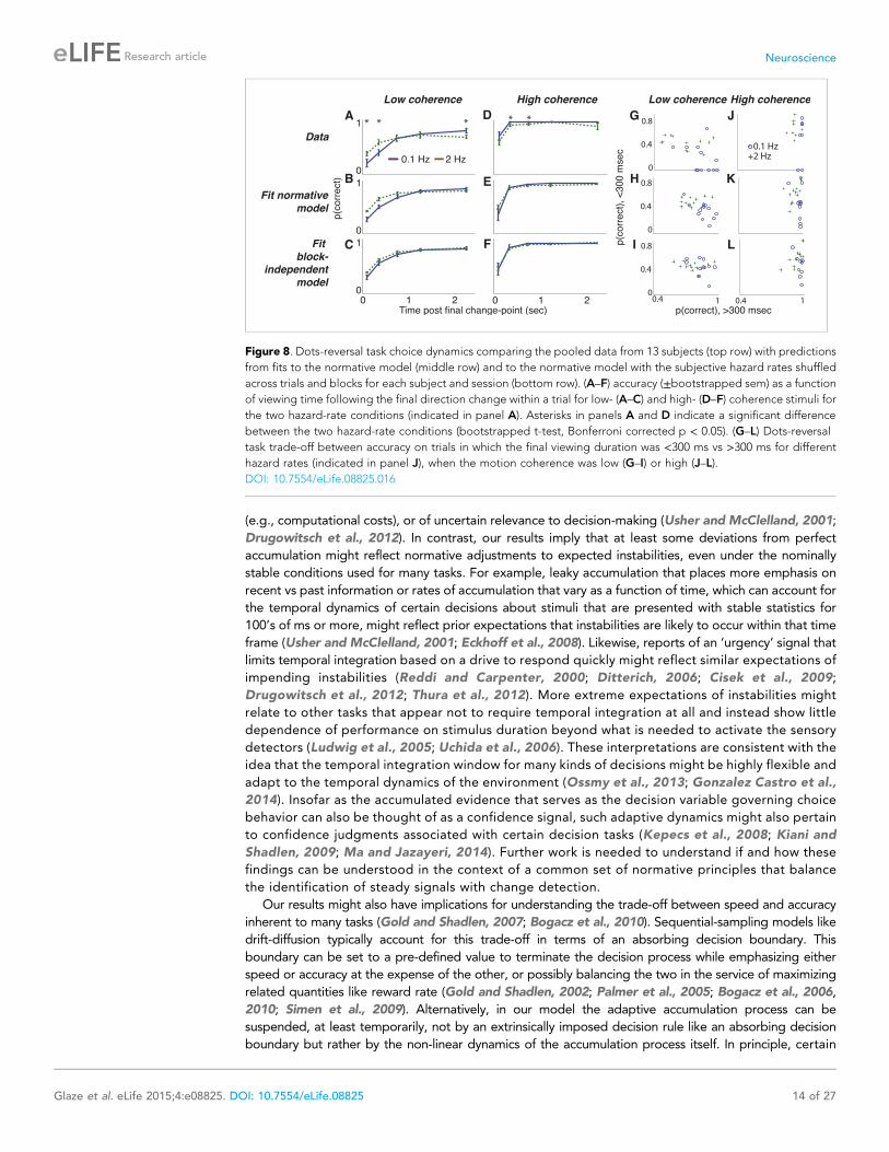
evidence. First, the choice data exhibited dynamics predicted by the normative model (Figure 8). For
high-coherence trials, the strong sensory evidence dominated the decision process, yielding >90%accuracy within 500 ms following the final change in direction irrespective of the rate of preceding
direction changes (Figure 8D,E). In contrast, for low-coherence trials, integration times were strongly
dependent on hazard rate (i.e., greater effects of ψ in Equation 1) Specifically, accuracy improved more
steeply as a function of viewing duration for the low- vs high-hazard condition: performance was worse
for the 0.1-Hz condition for durations <500 ms, reflecting persistence of the perceived direction of
motion just prior to the final change-point (i.e., direction reversal), but rose as viewing duration
increased and exceeded performance for the 2-Hz condition at long durations (Figure 8A,B). These
dynamics, particularly at low coherences, were not predicted by the block-independent model and thus
did not reflect uneven sampling of the data under the different coherence and hazard conditions
(Figure 8C,F).
Second, as with the triangles task, this decision process reflected a strong hazard- and evidence-
strength-dependent trade-off between detecting changes and identifying steady signals, as predicted
by the normative model (Figure 8G–K). For low-coherence trials, choice accuracy was lower for the
low-hazard condition just following a change-point (median ± bootstrapped SEM 7.1 ± 11.1% and
Figure 7. Dots-reversal task and normative model fits.
(A) Representation of a reversing-dots stimulus for
a single trial. The subject was instructed to indicate the
final, perceived direction of motion. (B) Subjective
hazard rate, estimated from direct fits of choice data by
the normative model with hazard rate as a free
parameter, plotted as a function of objective hazard
rate. Each pair of connected points represents data from
an individual subject.
DOI: 10.7554/eLife.08825.011
Glaze et al. eLife 2015;4:e08825. DOI: 10.7554/eLife.08825 11 of 27
Research article Neuroscience
40.3 ± 2.8%, for low- and high-hazard sessions
respectively, when the stimulus was shown for
<300 ms following the final change-point,
Wilcoxon signed rank, p < 0.01, vs predicted
accuracies of 34.6 ± 4.7% and 44.9 ± 3.1%,
respectively) but was greater for the low-hazard
condition thereafter (83.6 ± 3.6% and 69.9 ±8.3%, respectively, p < 0.0005, vs predicted
86.2 ± 2.3% and 74.2 ± 2.9%, respectively).
For high-coherence trials, choice accuracy was
much higher overall and, consistent with the
normative model, showed a weaker trade-off,
with no difference by hazard-rate condition for
short viewing durations following the final
change point (66.7 ± 14.6% and 66.1 ± 7.3%
for 0.1-Hz and 2-Hz sessions respectively,
p = 0.831, vs predicted 46.9 ± 9.4% and 59.7
± 3.7%, respectively) and only a slight difference
for longer post-change durations (100 ± 0% and
93.5 ± 1.4%, respectively, p = 0.004, vs predicted
97.8 ± 0.4% and 92.1 ± 2.0%, respectively).
In contrast, the block-independent model did
not predict these hazard-dependent trade-offs
(Figure 8I,L).
Third, we directly measured the dependence
of choice dynamics on both the hazard rate and
the strength of the sensory evidence by fitting
choice data to integrating models with separate
leaks for each hazard-specific session and co-
herence level (Figure 9). As predicted by the
normative model (Figures 3A, 8B,E), the best-
fitting leak depended on both (Friedman test, p < 0.0005 for the effect of hazard rate and p < 0.0001
for the effect of motion coherence; Figure 9A). The per-subject, pairwise differences between best-
fitting leak, computed with respect to either coherence or hazard rate, did not differ from predictions
of the normative model (median ± bootstrapped SEM normalized data–model difference by hazard
rate = −0.003 ± 0.021, by coherence = −0.001 ± 0.050, Wilcoxon signed rank p = 0.501 and 0.292,
respectively).
In contrast, the choice data from the dots-reversal task were not as well matched by either of
the two adaptive, suboptimal models we considered (Figure 3). The leaky-integrator model, in
which the leak depended on hazard rate but not coherence level, had worse overall fits to the
choice data than the normative model for 10 of 13 subjects (median ± bootstrapped SEM
difference in BIC = −4.066 ± 3.078, Wilcoxon signed rank, p < 0.05), failing in particular to
capture the strongly coherence-dependent leak of the data and the normative model
(Figure 9C,F,H,I; normalized data–model median ± bootstrapped SEM difference between
change in leak by coherence = 0.241 ± 0.067, Wilcoxon signed rank p < 0.0005). The normative
model also outperformed the model with perfect integration to a stabilizing boundary that freely
varied by objective hazard rate (BIC was lower for 9 of 13 subjects, −4.305 ± 2.662, p < 0.05). This
suboptimal model had a more subtle deviation from the data, consisting primarily of an
exaggerated dependence of leak on coherence (Figure 9D,G,J,K; per-subject, normalized
data–model difference between change in leak by coherence = −0.189 ± 0.059, Wilcoxon signed
rank p < 0.0001). Like for the normative fits, both suboptimal models also had best-fitting subjective
hazard rates that were imperfectly adapted to the objective values, further supporting the idea that
the subjects were using imperfect estimates to make their decisions (best-fitting λ = 0.789 ± 0.084
and 1.697 ± 0.227 Hz for the 0.1-Hz and 2-Hz conditions, respectively, for the leaky integrator and
4.378 ± 0.998 and 8.803 ± 1.159 Hz, respectively, for the perfect integrator to a stabilizing
boundary).
Video 1. Example random dot motion stimulus with
0.1 Hz changes, at 80% (‘high’) coherence.
DOI: 10.7554/eLife.08825.012
Video 2. Example random dot motion stimulus with
0.1 Hz changes, at 20% (‘low’) coherence.
DOI: 10.7554/eLife.08825.013
Glaze et al. eLife 2015;4:e08825. DOI: 10.7554/eLife.08825 12 of 27
Research article Neuroscience

DiscussionWe derived a normative model of evidence
accumulation for decision tasks that is based on
Bayesian principles for inferring changes in the
statistics of a generative process (Rabiner, 1989;
Adams and MacKay, 2007; Behrens et al.,
2007; Fearnhead and Liu, 2007; Brown and
Steyvers, 2009; Wilson and Finkel, 2009;
Nassar et al., 2010, 2012; Wilson et al., 2010;
Boerlin et al., 2013; Wilson et al., 2013;
Gonzalez Castro et al., 2014; McGuire et al.,
2014; Sato and Kording, 2014). Our model
incorporates change detection into sequential-
sampling decision models and is related to other,
modified versions of these models that have
been used to combine multiple sensory cues of
different but known reliabilities or infer unknown
sensory reliability assumed to be stable during
the course of decision-making (Hanks et al.,
2011; Deneve, 2012; Drugowitsch et al.,
2014). However, unlike those models, which
invoked a separate learning-rate term or had
other, more complex forms, our model casts
adaptation directly in the context of the
evidence-accumulation process that is a key focus
of studies of decision-making (Usher and McClel-
land, 2001; Roitman and Shadlen, 2002; Huk
and Shadlen, 2005; Uchida et al., 2006; Brunton
et al., 2013; Hanks et al., 2015). This formulation
allowed us to identify, for the first time, features of
evidence accumulation that can underlie normative, adaptive decision-making, including expectation-
dependent changes in leaky accumulation when beliefs are weak and saturating accumulation when
beliefs are stronger. We showed that human subjects made decisions on two separate tasks, requiring
evidence accumulation either across or within trials, that were consistent with the adaptive, hazard-
dependent accumulation process prescribed by the model.
Our findings substantially extend previous studies that similarly suggested that human
decision-making behavior can reflect adaptations to the rate of environmental changes (Behrens
et al., 2007; Brown and Steyvers, 2009; Gonzalez Castro et al., 2014). Specifically, we showed
that subjects could both learn a range of hazard rates and then use those learned rates in
a normative manner to interpret sequences of evidence to make decisions. However, they
tended to learn imperfectly, over-estimating low hazard rates and under-estimating high hazard
rates. Thus, although their use of these imperfectly learned hazard rates was consistent with the
normative model, their overall decisions in some cases fell short of the ideal observer. Our
framework provides a new way to interpret these deviations from optimality: not simply as poor
performance, but rather as different, hazard-dependent set-points of an inherent trade-off. This
tradeoff balances sensitivity to change during periods of expected instability, and sensitivity to steady-
state signals during periods of expected stability. These different set points may have reflected certain
prior expectations about the improbability of either perfect stability or excessive instability that could
constrain performance when those conditions occur.
Such prior expectations about a lack of perfect environmental stability interpreted in the context of
our framework might also provide new insights into previous studies of the temporal dynamics of
evidence accumulation. In some cases, decisions about perfectly stable stimuli appear to involve perfect
accumulation, as described by drift-diffusion and related models (Gold and Shadlen, 2000; Roitman
and Shadlen, 2002; Brunton et al., 2013; Hanks et al., 2015). Under those conditions, deviations from
perfect accumulation in the brain may be considered as inefficient, operating under other constraints
Video 3. Example random dot motion stimulus with 2
Hz changes, at 80% (‘high’) coherence.
DOI: 10.7554/eLife.08825.014
Video 4. Example random dot motion stimulus with 2
Hz changes, at 20% (‘low’) coherence.
DOI: 10.7554/eLife.08825.015
Glaze et al. eLife 2015;4:e08825. DOI: 10.7554/eLife.08825 13 of 27
Research article Neuroscience
(e.g., computational costs), or of uncertain relevance to decision-making (Usher and McClelland, 2001;
Drugowitsch et al., 2012). In contrast, our results imply that at least some deviations from perfect
accumulation might reflect normative adjustments to expected instabilities, even under the nominally
stable conditions used for many tasks. For example, leaky accumulation that places more emphasis on
recent vs past information or rates of accumulation that vary as a function of time, which can account for
the temporal dynamics of certain decisions about stimuli that are presented with stable statistics for
100’s of ms or more, might reflect prior expectations that instabilities are likely to occur within that time
frame (Usher and McClelland, 2001; Eckhoff et al., 2008). Likewise, reports of an ‘urgency’ signal that
limits temporal integration based on a drive to respond quickly might reflect similar expectations of
impending instabilities (Reddi and Carpenter, 2000; Ditterich, 2006; Cisek et al., 2009;
Drugowitsch et al., 2012; Thura et al., 2012). More extreme expectations of instabilities might
relate to other tasks that appear not to require temporal integration at all and instead show little
dependence of performance on stimulus duration beyond what is needed to activate the sensory
detectors (Ludwig et al., 2005; Uchida et al., 2006). These interpretations are consistent with the
idea that the temporal integration window for many kinds of decisions might be highly flexible and
adapt to the temporal dynamics of the environment (Ossmy et al., 2013; Gonzalez Castro et al.,
2014). Insofar as the accumulated evidence that serves as the decision variable governing choice
behavior can also be thought of as a confidence signal, such adaptive dynamics might also pertain
to confidence judgments associated with certain decision tasks (Kepecs et al., 2008; Kiani and
Shadlen, 2009; Ma and Jazayeri, 2014). Further work is needed to understand if and how these
findings can be understood in the context of a common set of normative principles that balance
the identification of steady signals with change detection.
Our results might also have implications for understanding the trade-off between speed and accuracy
inherent to many tasks (Gold and Shadlen, 2007; Bogacz et al., 2010). Sequential-sampling models like
drift-diffusion typically account for this trade-off in terms of an absorbing decision boundary. This
boundary can be set to a pre-defined value to terminate the decision process while emphasizing either
speed or accuracy at the expense of the other, or possibly balancing the two in the service of maximizing
related quantities like reward rate (Gold and Shadlen, 2002; Palmer et al., 2005; Bogacz et al., 2006,
2010; Simen et al., 2009). Alternatively, in our model the adaptive accumulation process can be
suspended, at least temporarily, not by an extrinsically imposed decision rule like an absorbing decision
boundary but rather by the non-linear dynamics of the accumulation process itself. In principle, certain
Figure 8. Dots-reversal task choice dynamics comparing the pooled data from 13 subjects (top row) with predictions
from fits to the normative model (middle row) and to the normative model with the subjective hazard rates shuffled
across trials and blocks for each subject and session (bottom row). (A–F) accuracy (±bootstrapped sem) as a function
of viewing time following the final direction change within a trial for low- (A–C) and high- (D–F) coherence stimuli for
the two hazard-rate conditions (indicated in panel A). Asterisks in panels A and D indicate a significant difference
between the two hazard-rate conditions (bootstrapped t-test, Bonferroni corrected p < 0.05). (G–L) Dots-reversal
task trade-off between accuracy on trials in which the final viewing duration was <300 ms vs >300 ms for different
hazard rates (indicated in panel J), when the motion coherence was low (G–I) or high (J–L).
DOI: 10.7554/eLife.08825.016
Glaze et al. eLife 2015;4:e08825. DOI: 10.7554/eLife.08825 14 of 27
Research article Neuroscience

Figure 9. Comparison of predictions from normative model vs from the suboptimal approximations (Figure 3)
for the dots-reversal task. (A–D) Parameter fits from a leaky-accumulator model with separate leak–rate
parameters per hazard rate (as indicated in panel B) and coherence (yielding four leaks per subject). (A) Leaks fit
to choice data. (B) Leaks fit to predicted choices from the normative model using best-fitting parameters from
subject data. (C) Leaks fit to predicted choices from the leaky-accumulator model using leaks that depended on
the session-specific hazard rate but not coherence. (D) Leaks fit to predicted choices from the bounded-
accumulator model using boundaries that depended on the session-specific hazard rate but not coherence.
(E–G) Difference in the best-fitting leak to the two coherences predicted by each of the models above plotted
against the difference in leaks from the direct fits to the choice data, separated by hazard rate (see panel B).
Differences are normalized by sum of leaks from each of the coherences. In A–G, each point represents a single
subject and hazard-rate condition. (H–K) Predicted accuracy (±bootstrapped sem) as a function of viewing time
following the final direction change within a trial for low- (H, J) and high- (I, K) coherence stimuli for the two
hazard-rate conditions (indicated in panel I), calculated as in Figure 8 but for predictions by fits to the leaky-
(H, I) and bounded- (J, K) accumulator models.
DOI: 10.7554/eLife.08825.017
Glaze et al. eLife 2015;4:e08825. DOI: 10.7554/eLife.08825 15 of 27
Research article Neuroscience
decisions might be made by committing to an alternative once this asymptotic regime is reached.
This regime represents an upper limit on the expected level of confidence and thus precludes the
need for either additional data for that alternative or for an additional boundary. In this case, the
resulting speed-accuracy trade-off would not necessarily reflect a pre-defined attempt to control
those factors explicitly but rather expectations about the rate at which the evidence-generating
process is changing.
Future work is needed to investigate how key features of our model might be implemented in the
nervous system for different tasks and different timescales. Previous studies using tasks that required
information accumulation on the timescale of the triangles task (e.g., over many seconds to minutes)
have similarly suggested that humans can approximate optimal change detection, which in some
cases includes a sensitivity to different hazard rates (Behrens et al., 2007; Brown and Steyvers,
2009; Nassar et al., 2010). The neural mechanisms of these abilities are not yet known, but fMRI
and pupillometry data suggest possible roles for the arousal system including the anterior
cingulate cortex and the noradrenergic system, and genotype data imply possible contributions
of the dopamine system (Yu and Dayan, 2005; Nassar et al., 2012; Behrens et al., 2007;
Krugel et al., 2009; O’Reilly et al., 2013; McGuire et al., 2014). Conversely, evidence-
accumulation processes that operate over shorter timescales, like for various versions of the
random-dot motion task, have focused on dynamic neural signals in other parts of cortex, the basal
ganglia, and the superior colliculus that can reflect the rapid build-up of evidence to select a particular
motor response (in these cases involving eye movements) (Gold and Shadlen, 2007; Ding and Gold,
2013). There are some suggestions that these systems may interact under certain conditions (O’Reilly
et al., 2013), but much more work is needed to understand the brain mechanisms responsible for the
kinds of normative, scale-invariant dynamics of evidence accumulation we characterized in this study.
Extending our framework to more than two alternatives and to conditions in which the statistics of
the evidence changes gradually, as opposed to abruptly, would also be an important step towards
better understanding how the brain accumulates and interprets dynamic evidence to solve complex,
real-world problems.
Materials and methods
Discrete-time modelThe normative model is based on the posterior probability each of option (z1 or z2) given all of
the evidence collected so far (x1:n), qðzinÞ≡pðzinjx1:nÞ. We assume that at each time step, there is
a probability (H, for ‘hazard rate’) that there will be a switch in the correct option. Beginning with
Bayes’ Rule, and using the sum and product rules of probability, it can be shown that:
qðz1nÞ∝pðxnjz1Þ�ð1−HÞq�z1;n−1�+Hq
�z2;n−1
��;
qðz2nÞ∝pðxnjz2Þ�Hq�z1;n−1
�+ ð1−HÞq�z2;n−1��; (5)
where p(xn|zi) is the likelihood of observing the evidence from source i. This relationship is the forward
recursion for the Baum-Welch algorithm in Hidden Markov Models and has been proven elsewhere
(Bishop, 2006). We derived the model (Equations 1, 2) by taking the logarithm of the ratio of the two
equations; that is, defining Ln ≡ logðqðz1nÞ=qðz2nÞÞ and expanding the logarithm, giving:
Ln = log½pðxnjz1Þ=pðxnjz2Þ�+ log��ð1−HÞq�z1;n−1�+Hq
�z2;n−1
����Hq�z1;n−1
�+ ð1−HÞq�z2;n−1���;
where the first term of the RHS is the LLR in Equation 1 by definition. The second term of the RHS
can be manipulated to yield ψ (Equation 2) first by dividing both the numerator and denominator by
Hq(z2,n − 1), then expanding the expression while usingqðz1;n−1Þqðz2;n−1Þ=expðLn−1Þ by definition, giving
ψðLn−1;HÞ= log
�1−HH expðLn−1Þ+ 1
�− log
�expðLn−1Þ+ 1−H
H
�. Factoring out exp(Ln − 1) from the first
term of the RHS yields Equation 2.
The special cases of H = 0 and H = 0.5 are most straightforward to see from Equation 5.
When H = 0:
Glaze et al. eLife 2015;4:e08825. DOI: 10.7554/eLife.08825 16 of 27
Research article Neuroscience

qðz1nÞ∝pðxnjz1Þq�z1;n−1
�;
qðz2nÞ∝pðxnjz2Þq�z2;n−1
�;
and
Ln = logðpðxnjz1Þ=pðxnjz2ÞÞ+ log�q�z1;n−1
��q�z2;n−1
��= LLRn + Ln−1;
which is perfect integration of the log likelihood ratios. When H = 0.5:
qðz1nÞ∝pðxnjz1Þ�0:5q
�z1;n−1
�+ 0:5q
�z2;n−1
��;
qðz2nÞ∝pðxnjz2Þ�0:5q
�z1;n−1
�+ 0:5q
�z2;n−1
��;
and
Ln = logðpðxnjz1Þ=pðxnjz2ÞÞ= LLRn:
Continuous-time modelAkin to the discrete-time model, the continuous-time version is based on the posterior probabilities of
each option given all evidence collected until a given time point t. It has been shown previously that
the non-normalized posterior probabilities of each of two states in a Markov jump process dx(t), with
average values ±μ and noise magnitude σ, can be written as a system of stochastic differential
equations (Zakai, 1965; Liptser and Shiryaev, 1977):
dq1ðtÞ= ½−λq1ðtÞ+ λq2ðtÞ�dt +q1ðtÞ μ
σ2dxðtÞ;
dq2ðtÞ= ½λq1ðtÞ− λq2ðtÞ�dt −q2ðtÞ μ
σ2dxðtÞ:
(6)
We used this result to write the log-odds ratio signal as L(t), seeking the derivative
dLðtÞ≡dlogðq1ðtÞ=q2ðtÞÞ, by beginning with Equation 6, separating out the deterministic and
stochastic components of the incoming evidence, and rewriting Equation 6 in vector form:
dqðtÞ=L+
μ
σ2DhðtÞ
qðtÞdt + μ
σDqðtÞdW ;
qðtÞ≡q1ðtÞ q2ðtÞ
TL≡
−λ λ
λ −λ
!D≡
1 0
0 −1
!:
(7)
.Applying It�o’s Lemma:
dLðtÞ=df ðqðtÞÞ=�ð∇f ÞT
L+
μ
σ2DhðtÞ
qðtÞ+ 1
2Tr
�μσDqðtÞ
T�∇2f
�μσDqðtÞ
��dt
+ :::ð∇f ÞTμσDqðtÞ
dW ;
f = logðq1ðtÞÞ− logðq2ðtÞÞ ∇f = ð 1=q1ðtÞ −1=q2ðtÞ ÞT
∇2f =
0@−1.ðq1ðtÞÞ2 0
0 1.ðq2ðtÞÞ2
1A :
(8)
We now expand each component of Equation 8, beginning with those in the deterministic
expression:
Glaze et al. eLife 2015;4:e08825. DOI: 10.7554/eLife.08825 17 of 27
Research article Neuroscience
ð∇f ÞTL+
μ
σ2DhðtÞ
qðtÞ=
1=q1ðtÞ −1=q2ðtÞ
"−λ+ hðtÞμ�σ2 λ
λ −λ− hðtÞμ�σ2#
q1ðtÞ q2ðtÞT
=
1=q1ðtÞ×�−λ+ hðtÞμ�σ2�×q1ðtÞ+ 1=q1ðtÞ× λ×q2ðtÞ+ :::
−1=q2ðtÞ× λ×q1ðtÞ− 1=q2ðtÞ×�−λ− hðtÞμ�σ2�×q2ðtÞ=
2hðtÞμ�σ2 + λðq2ðtÞ=q1ðtÞ−q1ðtÞ=q2ðtÞÞ;
(9)
and
1
2Tr
�μσDqðtÞ
T�∇2f
�μσDqðtÞ
�=
1
2
μσ
2q1ðtÞ −q2ðtÞ
−1.
q1ðtÞ2
0
0 1.ðq2ðtÞÞ2
!q1ðtÞ −q2ðtÞ
T=
1
2
μσ
2h−ðq1ðtÞÞ2
.ðq1ðtÞÞ2 + ðq2ðtÞÞ2
.ðq2ðtÞÞ2
i= 0:
(10)
Turning to the stochastic component:
ð∇f ÞTμσDqðtÞ
=μ
σ½1=q1ðtÞ −1=q2ðtÞ �
"q1ðtÞ 0
0 −q2ðtÞ
#
=μ
σ½q1ðtÞ=q1ðtÞ+q2ðtÞ=q2ðtÞ�= 2
μ
σ:
(11)
Substituting Equations 9–11 into Equation 8 yields:
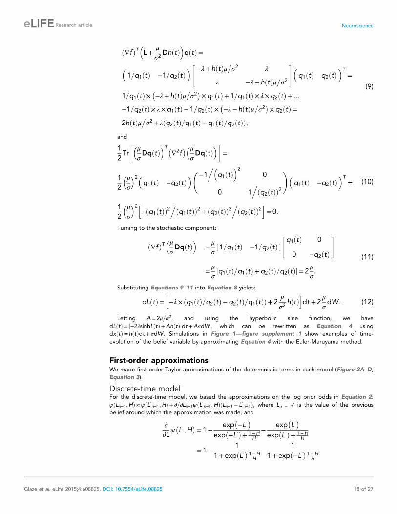
dLðtÞ=h−λ× ðq1ðtÞ=q2ðtÞ−q2ðtÞ=q1ðtÞÞ+ 2
μ
σ2hðtÞ
idt + 2
μ
σdW : (12)
Letting A= 2μ=σ2, and using the hyperbolic sine function, we have
dLðtÞ= ½−2λsinhLðtÞ+AhðtÞ�dt +AσdW , which can be rewritten as Equation 4 using
dxðtÞ=hðtÞdt + σdW . Simulations in Figure 1—figure supplement 1 show examples of time-
evolution of the belief variable by approximating Equation 4 with the Euler-Maruyama method.
First-order approximationsWe made first-order Taylor approximations of the deterministic terms in each model (Figure 2A–D,
Equation 3).
Discrete-time modelFor the discrete-time model, we based the approximations on the log prior odds in Equation 2:
ψðLn−1;HÞ≈ψðL′n−1;HÞ+ ∂=∂Ln−1ψðL′n−1;HÞðLn−1 − L′n−1Þ, where Ln − 1′ is the value of the previous
belief around which the approximation was made, and
∂∂L
ψ�L′;H
�= 1−
exp�−L′�
expð−L′Þ+ 1−HH
−exp
�L′�
expðL′Þ+ 1−HH
= 1−1
1+ expðL′Þ 1−HH
−1
1+ expð−L′Þ 1−HH
:
Glaze et al. eLife 2015;4:e08825. DOI: 10.7554/eLife.08825 18 of 27
Research article Neuroscience

Writing this equation with leak rate K and bias θ as in Equation 3, K ≡ 1−∂=∂LψðL′;HÞand θ≡ψðL′;HÞ−∂=∂LψðL′;HÞL′.
When previous beliefs are weak; that is, L′ = 0,
∂∂L
ψ�L′;H
�= 1−
1
1+ 1−HH
−1
1+ 1−HH
= 1−2H;
and
ψ�L′;H
�= L′ + log
�exp
�−L′�+1−H
H
�− log
�exp
�L′�+1−H
H
�
= log
�1+
1−H
H
�− log
�1+
1−H
H
�= 0:
Expressing the approximation in terms of Equation 3, leak rate K = 2H and bias θ = 0, as in
Equation 3a.
When previous beliefs are strongly in favor of the first alternative; that is, Ln − 1 → ∞,
limL′→∞
∂∂L
ψ�L′;H
�= 1− 0−
1
1+ 0× 1−HH
=0;
so the leak rate K = 1, and the bias is determined entirely by the value of the log-prior odds
evaluated as:
limL′→∞
�ψ�L′;H
��= L′ + log
�1−H
H
�− log
�exp
�L′��
= log
�1−H
H
�;
as in Equation 3b.
Similarly, when previous beliefs are strongly in favor of the second alternative; i.e., Ln − 1 → −∞,
limL′→−∞
∂∂L
ψ�L′;H
�= 1−
1
1+ 0× 1−HH
− 0= 0;
so the leak rate K = 1 here as well, and the bias is determined entirely by the value of the log-prior
odds evaluated as:
limL′→−∞
�ψ�L′;H
��= L′ + log
�exp
�−L′��
− log
�1−H
H
�=−log
�1−H
H
�;
as in Equation 3c.
Continuous-time modelWe approximated continuous-time model in Equation 4 by taking the first-order Taylor approximation
of the deterministic term, which we write here as gðLÞ≡ − 2λsinhðLÞ. Specifically, gðLÞ≈ kL+b, where k
represents the time-varying leak rate as in the discrete-time model (Figure 2B), and b represents a bias
in the derivative of the belief variable (Equation 4; Figure 2D) that, along with the changing leak rate,
effects a stabilizing boundary like in the discrete-time version. We calculated k as the slope of g(L), which
is given as 2λ×d=dLsinhðL′ðtÞÞ=2λcoshðL′ðtÞÞ, where L′ is the belief state around which the
approximation was made. We computed bias as: gðL′; λÞ− ∂∂L gðL′; λÞ× L′ =−2λsinhðL′Þ+2λL′coshðL′Þ.
Analogous to the discrete-time case, when L′ = 0 (certainty is low and beliefs are weak),
k =2λcoshð0Þ=2λ, b=−2λsinhð0Þ+2λ× 0× coshð0Þ= 0, and the approximation is linear, resulting in an
Ornstein-Uhlenbeck process during periods of stability in the data. However, as L′ → ±∞, k → ∞,
analogous to the leak rate approaching one in the discrete-time case, and
limL′→±∞
ðbÞ= limL′→±∞
�−2λsinh
�L′�+ 2λL′cosh
�L′��
=
limL′→±∞
�2λL′
�−sinh
�L′��
L′ + cosh�L′���
= limL′→±∞
�2λL′cosh
�L′��
→ ±∞:
Glaze et al. eLife 2015;4:e08825. DOI: 10.7554/eLife.08825 19 of 27
Research article Neuroscience
Whereas discrete-time approximations of the model give log-priors that are qualitatively similar to
Equation 2 for strong beliefs (Figure 1C), this regime in general is not as well approximated as a linear-
Gaussian process, with steady-state solutions over stable periods that are shifted, extreme-value
distributions (Figure 1—figure supplement 1, panel D). These distributions can be approximated by
first solving for the general steady-state probability distribution of L, as follows. Beginning with the
corresponding Fokker-Planck equation and letting p(L, t) denote the time-dependent probability
distribution of L and γ = Ah(t), the average of the sensory evidence during the stable period, we want
the solution to p(L, t) such that: ∂∂t pðL; tÞ=− ∂
∂L ð−2λsinhðLÞ+ γÞpðL; tÞ+ffiffiffiffiffiγ2
p∂2∂L2 pðL; tÞ=0.
Therefore, ∂∂L ð−2λsinhðLÞ+ γÞpðL; tÞ=
ffiffiffiffiffiγ2
p∂2∂L2 pðL; tÞ, which we solved as
pðLÞ=C0exp
R LLa
−2λsinhðLÞ+ γffiffiffiffiγ2
p dL
!, where C0 is a normalizing constant and La is a reflecting boundary
condition. So pðLÞ=C0expð−2λcoshðLÞ+ γL+2λcoshðLaÞ− γLaÞ=
ffiffiffiffiffiγ2
p and letting C be another
normalizing constant that absorbs the constant terms inside the exponential:
pðLÞ=Cexpð−2λcoshðLÞ+ γLÞ
. ffiffiffiffiffiγ2
p : (13)
In the high-certainty regime (the expected value of the belief variable is very positive or negative,
either because of strong sensory evidence or a very low hazard rate, or both), this expression can be
well approximated as
pðLÞ≈Cexpðð−λexpðLÞ+ γLÞ=γÞ when LðtÞ≫0; (14a)
pðLÞ≈Cexpðð−λexpð−LÞ+ γLÞ=−γÞwhen LðtÞ≪0: (14b)
Figure 1—figure supplement 1, panel B shows an example of this approximation along with
simulations. Equation 14 can be rewritten as extreme value distributions with location
parameters ±log(γ/λ) with the sign depending on the sign of the sensory evidence, and scale
parameter = 1. For example, taking Equation 14a,
Cexpðð−λexpðLÞ+ γLÞ=γÞ=Cexp
�−λ
γexpðLÞ+ L
�=
Cexpð−expðL− logðγ=λÞÞ+ L− logðγ=λÞ+ logðγ=λÞÞ=C′expð−expðL− logðγ=λÞÞ+ L− logðγ=λÞÞ;
where C′ = Cγ/λ.
Tasks48 subjects (29 female, 19 male; age range = 19–45 years) participated in the triangles task, and
13 subjects (7 female, 6 male; age range = 19–38 years) participated in the dots-reversal task
after providing informed consent. Human subject protocols were approved by the University
of Pennsylvania Internal Review Board. Both tasks were performed on an iMac with a 27′′(68.5 cm) screen.
Triangles taskTriangles were separated by 16 cm and represented the centers of a pair of two-dimensional
Gaussian distributions. On each trial, one triangle was chosen as the true source of the
generated star, and that source’s associated two-dimensional distribution was sampled to
determine the position of the star. Distributions were directly represented on the screen by
scaling the color axis by screen position between blue and green according to the probability
that a star would be generated in the given position (Figure 4A,B). Because the triangles were
separated along the horizontal axis, only this dimension was relevant for determining which
triangle represented the true source on that trial. For each trial, the star blinked on and off for
∼1.5 s before the subject could choose the inferred source of that star, to minimize fast guesses.
For each session, one of three different variances of the pair of two-dimensional distributions
was randomly chosen without replacement (the ratio of the standard deviation of the generative
Glaze et al. eLife 2015;4:e08825. DOI: 10.7554/eLife.08825 20 of 27
Research article Neuroscience
process to the distance between the triangles was 0.24, 0.33, or 0.41). These three conditions
corresponded to mean values of log-likelihood ratios of 9, 4.5, or 3.33, respectively, of
generated stars.
Each subject performed two 1000-trial blocks per session in 1–4 total sessions. Each block used
a hazard rate that governed the rate of switching between the two sources (triangles) and was chosen
randomly from a set of seven possible values (0.05, 0.1, 0.3, 0.5, 0.7, 0.9, 0.95). Hazard rates were
chosen without replacement within sessions to ensure a change across blocks. In a subset of sessions,
each block began with 400 trials in which subjects received feedback on the correct choice, followed
by another 400 trials without feedback and ending with 200 feedback-based trials so that changes in
hazard rate did not coincide with the onset of feedback.
Before each session, subjects were instructed that the triangles generated stars into overlapping
neighborhoods and shown representations of the spatial distributions. They were then instructed that
triangles would ‘take turns’ generating stars, with switches in the turn-taking that would occasionally
be fast or slow. After receiving these instructions, subjects were shown an animation illustrating the
generative process (i.e., a sample sequence of trials).
Subjects were paid a minimum $8 per session and an additional amount based on performance:
at the beginning of each session, the subject had $5, and over the trials was penalized by 20 cents
for each incorrect choice and rewarded with either 1 or 2 cents for correct choices. Total cash
reward was continuously updated on feedback trials but not on non-feedback trials so subjects
could not infer the previous correct choice. On average, subjects received a total additional cash
reward of $8 (range $0–27).
Dots-reversal taskThis task was based on decisions about the coherent direction of motion of a set of stochastic dots
(density = 70 dots/deg2/s) presented in a 10˚-diameter circular aperture at the center of the computer
screen with three interleaved frames of motion. Each trial involved a stimulus 5–10 s in duration,
determined as min(10, 5 + τ), where τ was an exponentially distributed random variable, making trial
terminations unpredictable within the given time frame. Within each trial, the direction of movement
alternated between leftward and rightward at an average hazard rate of either 0.1 Hz or 2 Hz. Subjects
participated in two sessions each, with 200 trials per session and a hazard rate that was constant
throughout the session. The order of the two hazard rate sessions was chosen at random.
Each session began with 20 practice trials in which coherence was set to 60–85%, relatively high
values that were considered easy for all subjects. For the remaining 180 trials, coherence was randomly
chosen as either this ‘high coherence’ value (25% of trials) or a ‘low-coherence’ value (75% of trials).
The value used for ‘low coherence’ was determined separately for each subject (mean ± SEM =14.85 ± 1.53%, range 6–38%), corresponding to the coherence for which the participant could
correctly decide the direction of a 500-ms long stable stimulus (i.e., no direction changes) 65% of
the time. We assessed this threshold using a modified version of the adaptive QUEST procedure in
which coherence was set to the mean of the threshold probability distribution (Watson and Pelli,
1983; King-Smith et al., 1994). We ran the QUEST procedure before each session and did not
end the procedure until stable performance was achieved, defined as an estimated threshold log-
likelihood ≥ −2.5 under the assumption that unstable performance would shift the corresponding
threshold and keep log-likelihoods lower (direct estimates of threshold across consecutive 20-trial
blocks verified this assumption). We also ensured that the measured threshold from this procedure
was consistent across sessions for individual subjects. We based ‘high’ coherence on the low-coherence
threshold: subjects with thresholds >15% received 85% high coherence, those with thresholds between
7–15% received 80% high coherence, and one subject with a remarkably low (∼4–5%) threshold
received 60% high coherence. All stimuli in this range are fairly easy to judge.
Before the session, subjects were instructed to do their best to follow motion direction throughout
a given trial and indicate the direction they believed dots were moving in at the ‘very end’ of the trial.
Subjects received feedback after each trial on the correct answer but were not given additional
monetary reward for performance as in the triangles task.
Model fittingAll models were fit to choice data using Matlab’s optimization toolbox by minimizing the cross-entropy
error function (Bishop, 2006):
Glaze et al. eLife 2015;4:e08825. DOI: 10.7554/eLife.08825 21 of 27
Research article Neuroscience

e=−∑nð1− ρnÞlogð1−bρnÞ+ ρnlogðbρnÞ; (15)
where ρn is a binary variable indicating which alternative was chosen on trial n (arbitrarily defined as 0 for
the right and 1 for the left) and bρn is the choice probability predicted by the given model. All models
assumed the choices were based on the sign of the subjective log-odds.
Triangles taskWe fit choices from the triangles task for each block of trials and each session by computing
estimated Ln on each iteration of the fitting algorithm using Equation 1; the current best estimate of
subjective hazard rate for that iteration and block of trials ( bHb); and a gain term on star position
(β) that was applied across blocks but was specific to each session, which accounted for a subjective
estimate of the generative variance (Gold and Shadlen, 2001): Ln =ψðLn−1; bHbÞ+ βxn. Unless
otherwise indicated, all fits were made to trials without any feedback on the correct answer to
confirm that learned hazard rates were used during this period. We omitted from further analyses
the first 200 trials of each block for sessions in which no trial-by-trial feedback was given at all,
allowing for stabilization of learned, subjective estimates of the current generative H and resulting in
a total of 800–6400 trials per subject for analysis. We assumed choices were based on the subjective
log-odds and Gaussian noise: ρn = signðLn + ζnÞ where ςn is the Gaussian noise variable. We also
assumed a fixed magnitude of noise υ across sessions but specific to each subject. Model fits thus
computed the cumulative probability of choosing the left triangle for subject i, in session s, block b,
and trial n as:
bpi;s;b;n =1
2+1
2erfLi;s;b;n
. ffiffiffi2
pυi; Li;s;b;n =ψ
Li;s;b;n−1; bHib
+ βxn: (16)
Thus, this model had 4–16 free parameters for each subject, depending on the number of sessions.
Because of the large number of parameters for some subjects, we used a maximum a posteriori (MAP)
fitting procedure that placed conjugate priors on each parameter that were fixed across subjects and
conditions, subtracting off log(p[parameter estimate|conjugate prior distribution of parameters]) from
the error term in Equation 15.
Dots-reversal taskWe fit the continuous-time model to data from the dots-reversal task using Equation 1, which is the
most efficient discrete-time approximation of Equation 4 and faster than the Euler-Maruyama
approximation with small time-steps. However, unlike the triangles task, here all choices were made
after observing an entire sequence of stimuli over the trial. We thus fit the model using Equation 1 with
n indexing trial rather than time andm indexing time-step within a trial, i indexing subject and s indexing
session, as follows:
Lismn =ψLis;m−1;n; bHis
+ kiCismn +
ffiffiffiffiffiffiffiffiffiffiffiffiffiffiffiffiffiffiffiffi2kiÆjCisnjæ
pηismn; (17)
where ki is a gain term for that subject on signed coherence Cismn (negative for rightward motion,
positive for leftward motion; because coherence was determined probabilistically, its magnitude
could vary step-by-step within a trial); ÆjCisnjæ indicates the expected coherence magnitude for that
trial, determined experimentally as described above; ηismn is zero-mean, unit variance Gaussian noise;
and bHis is subjective hazard rate specific to each session. To convert to a continuous-time subjective
hazard rate λ, we multiplied bHis by the monitor refresh rate (60 Hz), which determines the time-steps
between dot drawings.
The last two terms of Equation 17 represent the subjective LLR, which we assume reflects
a coherence-dependent signal (the second-to-last term) plus internal (neural), signal-dependent noise
(the last term). Because we could not directly observe this noisy quantity, we fit the model by
numerically deriving the time-evolution of the log-odds probability distribution over each trial and
each step of the fitting iteration. Specifically, we determined the probability of each log-odds (Lisomn)
at each time step by marginalizing over the probability of each log-odds from the previous time-step
(Lisj, m − 1, n):
Glaze et al. eLife 2015;4:e08825. DOI: 10.7554/eLife.08825 22 of 27
Research article Neuroscience

pðLisomnÞ=Z ∞
−∞NLo
���ψLj; bHis
+ kiCismn;
ffiffiffiffiffiffiffiffiffiffiffiffiffiffiffiffiffiffiffiffi2kiÆjCisnjæ
p p�Lisj;m−1;n
�dLj; (18)
where Nðxjμ; σÞ denotes a Gaussian probability distribution function of variable x with mean μ and
standard deviation σ and is the conditional probability distribution of the log-odds on each time-step
given the coherence, model parameters, and log-odds on the previous time-step. Probability
distributions were initialized on each trial as a Dirac delta function. For the model fits, we discretized
the log-odds space between −10 and 10 over steps of 0.4 log-odds, which we determined via
simulations to be a sufficient range and resolution for accurate parameter estimates. Estimated choice
probabilities were then computed as the cumulative probability of choosing the leftward direction:bpisn =R∞0 pðLisMnÞdLi . Model fits were thus based on three parameters per subject, a single gain term ki
and two hazard rate terms bHis, one for each session.
Sub-optimal model #1: block-independent modelFor both tasks, we fit to choice data a version of the normative model that ignored the block-wise
changes in objective hazard rate. To ensure a fair model comparison with the block-dependent normative
model, we constructed the null model using the same number of hazard-rate parameters but randomly
shuffled across blocks. Specifically, for the triangles task the main model equation (Equation 16) was
written as Lisbn =ψðLisb;n−1; bHis;bðnÞÞ+ βisxisbn, where b(n) denotes the hazard-specific block to which this
trial was randomly assigned. Randomization was performed before each fit, and this shuffle-and-fit
procedure was repeated 50 times to generate a distribution of model log-likelihoods and BIC values
against which the normative model could be compared across subjects. For the dots-reversal task, the
main model equations (Equations 17, 18) were written as Lmn =ψðLm−1;n; bHðsnÞÞ+ kCmn +ffiffiffiffiffiffiffiffiffiffiffiffiffiffiffiffiffi2kÆjCnjæ
pηmn,
where s was a vector indicating the randomized session, with the shuffle-and-fit procedure repeated 20
times per subject.
Sub-optimal model #2: block-dependent leaky accumulatorFor both tasks, we also fit an alternative model based on the linear approximation in Equation 3a.
For the triangles task this model was written as Lisbn = ð1−KisbÞLisb;n−1 + βisxisbn, where K was the leak
specific to subject i in session s and block b, and the other parameters were as described above. For the
dots-reversal task we fit the same model, only here treating noise as a latent variable like we did for
fitting the normative model and deriving the time-evolution of the log-odds probability distribution over
each trial and each step of the fitting iteration: Lismn = ð1−KisÞLism−1;n + kiCismn +ffiffiffiffiffiffiffiffiffiffiffiffiffiffiffiffiffiffiffiffi2kiÆjCisnjæ
pηismn. Unlike
the normative model, these fits were greatly simplified by an analytic solution for the stationary standard
derivation of the log-odds, given the current coherence and model parameters: σisn =ffiffiffiffiffiffiffiffiffiffiffiffiffiffiffiffiffiffiffiffiffiffiffiffiffikiÆjCisnjæ=Kis
p.
This quantity is the standard deviation for the stationary probability distribution of the discrete-time
analogue of an Ornstein-Uhlenbeck process in which coherence is perfectly stable over a trial. Thus, for
each step of the fitting procedure, we solved for the average log-odds at the end of the trial by:
(1) running the deterministic portion of the leaky-accumulation over the time-dependent coherence for
the trial, and (2) writing the probability distribution of the log-odds at the end of the trial as a Gaussian
with the final mean determined in step 1 and a standard deviation as described above, givingbpi;s;n =12+
12 erfðLi;s;M;n=
ffiffiffiffiffiffiffiffiffiffiffiffiffiffiffiffiffiffiffiffiffiffiffiffiffiffiffiffi2kiÆjCisnjæ=Kis
p Þ, where M indicates the final sample of trial n.
Sub-optimal model #3: perfect accumulation with block-dependentstabilizing boundariesFor both tasks, we also fit an alternative model assuming perfect integration to a stabilizing boundary as
in Equation 2 with the boundary in Equation 3b,c as a free parameter; that is, rewriting Equation 2 as:
ψðLn−1;HÞ=
8>><>>:Ln−1 −θ< Ln−1 < θ
θ Ln−1 ≥ θ
−θ Ln−1 ≤ − θ
;
θ= log
�1−H
H
�:
(19)
Glaze et al. eLife 2015;4:e08825. DOI: 10.7554/eLife.08825 23 of 27
Research article Neuroscience

For the triangles task, these fits were made as for the normative model, only using the re-written
expression in Equation 19 for log-prior odds above; that is, Lisbn =ψðHisb; Lisb;n−1Þ+ βisxisbn. For the
dots-reversal task, we similarly made fits as for the normative model, substituting the expression for ψ
in Equation 19 into Equations 17, 18.
Analysis detailsChoice data shown in Figure 5A were fit by a two-parameter logistic function:bρn =1=½1+expððLLRn −ϕÞ=βÞ�, where ϕ represents the LLR for which subjects have a 50% chance
of choosing either side, and β is the slope of the function around that point. Average differences in
parameter ϕ by hazard-rate condition are reflected in the horizontal shift of the psychometric function,
representing a bias towards (leftward shift) or away from (rightward shift) repeating the same choice.
Like for the fits of the main normative model, here the first 200–400 trials of each block were excluded
to allow for a period of learning. We report the correlation between ϕ and the prediction from the
asymptotic approximation of the fit normative model: logðð1−HsubjÞ=HsubjÞ.The subjective mappings of ψn to Ln − 1 in Figure 6 were estimated as a non-parametric function, fit
to choice data based on Ln = bψðLn−1Þ+ LLRn where here the LLR was based on the generative variance
used for the task. We expressed ψn as an interpolated function of Ln − 1, with values spread evenly
between −10 and 10 in steps of one log-odds ratio and interpolation performed with cubic splines.
We fit the mapping with the same objective function as for the parametric models (Equation 10),
using the entire data set within a given block to estimate the ψ that best fit choice data. We used
Tikhonov regularization of the derivative (for smoothness) using the added penalty term: γ∑iðΔψ iÞ2,where i indexes the value of L for which ψ was estimated and γ = 1/20 was determined through ad
hoc methods.
Standard errors and statistical tests on performance measured as a function of viewing duration
following the final change-point on the dots-reversal task were based on bootstrapped samples of the
behavioral data or model predictions (Figure 8A–F, Figure 9H–K). Viewing duration bins were 0–200,
200–500, 500–1000, 1000–1500 and 1500–3000 ms. These analyses only included trials for which there
was at least one change-point and the duration of the second-to-last direction was at least 300 ms to
avoid immediately sequential change-points. The mean ± SEM durations of the second-to-last
direction for trials used in this analysis were 2945 ± 55 ms for 0.1 Hz and 789 ± 13 ms for 2 Hz. At these
durations, discrimination accuracy was likely to be at nearly asymptotic levels at the time of the final
change-point. For a given duration bin specific to coherence and condition (indexed jointly as k),
a single bootstrapped sample m of performance was calculated as ρkm = ð∑nρkmnÞ=Nkm, where m
indexes subject, generated as a random integer between zero and 14; n indexes trial; and Nkm is
the total number of trials within the duration bin for that subject and trial type (e.g., 0.1 Hz,
low coherence). Means and standard errors were calculated as means and standard deviations
of all bootstrapped samples (1000 samples per comparison). Statistical tests between
condition-by-coherence trials i and j were based on paired differences between the same
bootstrapped samples. The probability that ρi > ρj was calculated as 1M∑mðρim − ρjm > 0Þ, (where M
was the total number of bootstrapped samples for that comparison), likewise for ρi < ρj , and
statistical significance indicated when one of these was less than the desired confidence
level (0.05).
Fit leaks for the dots-reversal task (Figure 9) used the same algorithm as in the leaky-accumulator
model described above but with separate leak terms for both hazard rate and low vs high coherence.
Specifically, for subject i, session s, time-step m, trial n, and coherence level c, we defined the leak
Lismn = ð1−KiscÞLism−1;n + kiCismn +ffiffiffiffiffiffiffiffiffiffiffiffiffiffiffiffiffiffiffiffi2kiÆjCisnjæ
pηismn. The noise was based on the stationary standard
derivation of the log-odds, given the current coherence and model parameters: σisn =ffiffiffiffiffiffiffiffiffiffiffiffiffiffiffiffiffiffiffiffiffiffiffiffiffiffiffikiÆjCisnjæ=Kisc
p.
We then fit the choice data to the predicted probability of a given choice for each trial,bpi;s;n =12+
12 erfðLi;s;M;n=
ffiffiffiffiffiffiffiffiffiffiffiffiffiffiffiffiffiffiffiffiffiffiffiffiffiffiffiffiffiffi2kiÆjCisnjæ=Kisc
p Þ, where M indicates the final sample of trial n. We used a beta
distribution prior on leak rate, letting the maximized model log probability for each subject be based
on the sum of log likelihoods and this log prior probability, similar to what we did for the triangles task.
We were interested in the dependence of leak on coherence level and comparing these dependencies
between the choice data and model predictions. To control for overall level of leak by session (and
subject), we computed the dependence as a normalized quantity: dis = ðKis;high −Kis;lowÞ=ðKis;high +Kis;lowÞwhere the ‘high’ and ‘low’ subscripts denote leaks for high and low coherences. The comparison
Glaze et al. eLife 2015;4:e08825. DOI: 10.7554/eLife.08825 24 of 27
Research article Neuroscience

between the data and normative model prediction of the dependence on hazard rate (session) used an
analogous normalized measure: dis = ðKis;fast −Kis;slowÞ=ðKis;fast +Kis;slowÞ where ‘fast’ and ‘slow’ indicate
the 2 Hz and 0.1 Hz sessions respectively. Statistics reported were based on these difference measures.
AcknowledgementsWe thank Gabriel Kroch and Timothy Kim for help with data collection and Joe McGuire, Yin Li, Matt
Nassar, and Bob Wilson for comments.
Additional information
Funding
Funder Grant reference Author
National Institutes ofHealth (NIH)
OppNet Grant R01MH098899
Christopher M Glaze,Joseph W Kable, Joshua IGold
The funder had no role in study design, data collection and interpretation, or thedecision to submit the work for publication.
Author contributions
CMG, Conception and design, Acquisition of data, Analysis and interpretation of data, Drafting or
revising the article; JWK, JIG, Conception and design, Analysis and interpretation of data, Drafting
or revising the article
Ethics
Human subjects: Informed consent, and consent to publish, was obtained from each subject prior to
each experiment. Human subject protocols were approved by the University of Pennsylvania Internal
Review Board.
ReferencesAdams RP, MacKay DJ. 2007. Bayesian online changepoint detection. University of Cambridge Technical report.Barnard GA. 1946. Sequential tests in industrial statistics. Journal of the Royal Statistical Society 8:1–26. doi: 10.2307/2983610.
Behrens TE, Woolrich MW, Walton ME, Rushworth MF. 2007. Learning the value of information in an uncertainworld. Nature Neuroscience 10:1214–1221. doi: 10.1038/nn1954.
Bishop CM. 2006. Pattern recognition and machine learning. New York: Springer.Boerlin M, Machens CK, Deneve S. 2013. Predictive coding of dynamical variables in balanced spiking networks.PLoS computational biology, 9(11):p. e1003258.
Bogacz R, Brown E, Moehlis J, Holmes P, Cohen JD. 2006. The physics of optimal decision making: a formalanalysis of models of performance in two-alternative forced choice tasks. Psychological Review 113:700–765.doi: 10.1037/0033-295X.113.4.700.
Bogacz R, Wagenmakers EJ, Forstmann BU, Nieuwenhuis S. 2010. The neural basis of the speed-accuracy tradeoff.Trends in Neurosciences 33:10–16. doi: 10.1016/j.tins.2009.09.002.
Britten KH, Shadlen MN, Newsome WT, Movshon JA. 1992. The analysis of visual motion: a comparison ofneuronal and psychophysical performance. The Journal of Neuroscience 12:4745–4765.
Brown SD, Steyvers M. 2009. Detecting and predicting changes. Cognitive Psychology 58:49–67. doi: 10.1016/j.cogpsych.2008.09.002.
Brunton BW, Botvinick MM, Brody CD. 2013. Rats and humans can optimally accumulate evidence for decision-making. Science 340:95–98. doi: 10.1126/science.1233912.
Busemeyer JR, Townsend JT. 1993. Decision field theory: a dynamic-cognitive approach to decision making in anuncertain environment. Psychological Review 100:432–459. doi: 10.1037/0033-295X.100.3.432.
Cisek P, Puskas GA, El-Murr S. 2009. Decisions in changing conditions: the urgency-gating model. The Journal ofNeuroscience 29:11560–11571. doi: 10.1523/JNEUROSCI.1844-09.2009.
Clifford CW, Ibbotson MR. 2002. Fundamental mechanisms of visual motion detection: models, cells and functions.Progress in Neurobiology 68:409–437. doi: 10.1016/S0301-0082(02)00154-5.
Crisan D, Rozovskii B. 2011. The Oxford handbook of nonlinear filtering. New York: Oxford University Press.Deneve S. 2012. Making decisions with unknown sensory reliability. Frontiers in Neuroscience 6:75. doi: 10.3389/fnins.2012.00075.
Ding L, Gold JI. 2013. The basal ganglia’s contributions to perceptual decision making. Neuron 79:640–649.doi: 10.1016/j.neuron.2013.07.042.
Glaze et al. eLife 2015;4:e08825. DOI: 10.7554/eLife.08825 25 of 27
Research article Neuroscience

Ditterich J. 2006. Evidence for time-variant decision making. The European Journal of Neuroscience 24:3628–3641. doi: 10.1111/j.1460-9568.2006.05221.x.
Drugowitsch J, DeAngelis GC, Klier EM, Angelaki DE, Pouget A. 2014. Optimal multisensory decision-making ina reaction-time task. eLife 3:e03005. doi: 10.7554/eLife.03005.
Drugowitsch J, Moreno-Bote R, Churchland AK, Shadlen MN, Pouget A. 2012. The cost of accumulating evidence inperceptual decision making. The Journal of Neuroscience 32:3612–3628. doi: 10.1523/JNEUROSCI.4010-11.2012.
Eckhoff P, Holmes P, Law C, Connolly PM, Gold JI. 2008. On diffusion processes with variable drift rates as modelsfor decision making during learning. New Journal of Physics 10:nihpa49499. doi: 10.1088/1367-2630/10/1/015006.
Fearnhead P, Liu Z. 2007. On-line inference for multiple changepoint problems. Journal of the Royal StatisticalSociety: Series B 69:589–605. doi: 10.1111/j.1467-9868.2007.00601.x.
Gold JI, Shadlen MN. 2000. Representation of a perceptual decision in developing oculomotor commands. Nature404:390–394. doi: 10.1038/35006062.
Gold JI, Shadlen MN. 2001. Neural computations that underlie decisions about sensory stimuli. Trends in CognitiveSciences 5:10–16. doi: 10.1016/S1364-6613(00)01567-9.
Gold JI, Shadlen MN. 2002. Banburismus and the brain: decoding the relationship between sensory stimuli,decisions, and reward. Neuron 36:299–308. doi: 10.1016/S0896-6273(02)00971-6.
Gold JI, Shadlen MN. 2007. The neural basis of decision making. Annual Review of Neuroscience 30:535–574.doi: 10.1146/annurev.neuro.29.051605.113038.
Gonzalez Castro LN, Hadjiosif AM, Hemphill MA, Smith MA. 2014. Environmental consistency determines the rateof motor adaptation. Current Biology 24:1050–1061. doi: 10.1016/j.cub.2014.03.049.
Good IJ. 1979. Studies in the history of probability and statistics. XXXVI. AM Turing’s statistical work in World WarII. Biometrika 66:393–396. doi: 10.1093/biomet/66.2.393.
Green DM, Swets JA. 1966. Signal detection theory and psychophysics. New York: John Wiley & Sons.Hanks TD, Kopec CD, Brunton BW, Duan CA, Erlich JC, Brody CD. 2015. Distinct relationships of parietal andprefrontal cortices to evidence accumulation. Nature 520:220–223. doi: 10.1038/nature14066.
Hanks TD, Mazurek ME, Kiani R, Hopp E, Shadlen MN. 2011. Elapsed decision time affects the weighting of priorprobability in a perceptual decision task. The Journal of Neuroscience 31:6339–6352. doi: 10.1523/JNEUROSCI.5613-10.2011.
Henning GB, Hertz BG, Broadbent DE. 1975. Some experiments bearing on the hypothesis that the visual systemanalyses spatial patterns in independent bands of spatial frequency. Vision Research 15:887–897. doi: 10.1016/0042-6989(75)90228-X.
Huk AC, Shadlen MN. 2005. Neural activity in macaque parietal cortex reflects temporal integration of visualmotion signals during perceptual decision making. The Journal of Neuroscience 25:10420–10436. doi: 10.1523/JNEUROSCI.4684-04.2005.
Kepecs A, Uchida N, Zariwala HA, Mainen ZF. 2008. Neural correlates, computation and behavioural impact ofdecision confidence. Nature 455:227–231. doi: 10.1038/nature07200.
Kiani R, Shadlen MN. 2009. Representation of confidence associated with a decision by neurons in the parietalcortex. Science 324:759–764. doi: 10.1126/science.1169405.
King-Smith PE, Grigsby SS, Vingrys AJ, Benes SC, Supowit A. 1994. Efficient and unbiased modifications of theQUEST threshold method: theory, simulations, experimental evaluation and practical implementation. VisionResearch 34:885–912. doi: 10.1016/0042-6989(94)90039-6.
Krugel LK, Biele G, Mohr PN, Li SC, Heekeren HR. 2009. Genetic variation in dopaminergic neuromodulationinfluences the ability to rapidly and flexibly adapt decisions. Proceedings of the National Academy of Sciences ofUSA 106:17951–17956. doi: 10.1073/pnas.0905191106.
Lasley DJ, Cohn T. 1981. Detection of a luminance increment: effect of temporal uncertainty. Journal of the OpticalSociety of America 71:845–850. doi: 10.1364/JOSA.71.000845.
Link SW. 1992. The wave theory of difference and similarity. Hillsdale, NJ: Erlbaum.Liptser RS, Shiryaev AN. 1977. Statistics of random processes: 1. General theory. New York: Springer-Verlag.Luce RD. 1986. Response times: their role in inferring elementary mental organization. New York: Oxford UniversityPress.
Ludwig CJ, Gilchrist ID, McSorley E, Baddeley RJ. 2005. The temporal impulse response underlying saccadicdecisions. The Journal of Neuroscience 25:9907–9912. doi: 10.1523/JNEUROSCI.2197-05.2005.
Ma WJ, Jazayeri M. 2014. Neural coding of uncertainty and probability. Annual Review of Neuroscience 37:205–220. doi: 10.1146/annurev-neuro-071013-014017.
Macmillan NA, Creelman CD. 2004. Detection theory: a user’s guide. Mahwah, NJ: Lawrence Erlbaum.McGuire JT, Nassar MR, Gold JI, Kable JW. 2014. Functionally dissociable influences on learning rate in a dynamicenvironment. Neuron 84:870–881. doi: 10.1016/j.neuron.2014.10.013.
Nachmias J, Rogowitz BE. 1983. Masking by spatially-modulated gratings. Vision Research 23:1621–1629. doi: 10.1016/0042-6989(83)90176-1.
Nassar MR, Rumsey KM, Wilson RC, Parikh K, Heasly B, Gold JI. 2012. Rational regulation of learning dynamics bypupil-linked arousal systems. Nature Neuroscience 15:1040–1046. doi: 10.1038/nn.3130.
Nassar MR, Wilson RC, Heasly B, Gold JI. 2010. An approximately Bayesian delta-rule model explains the dynamicsof belief updating in a changing environment. The Journal of Neuroscience 30:12366–12378. doi: 10.1523/JNEUROSCI.0822-10.2010.
O’Reilly JX, Schuffelgen U, Cuell SF, Behrens TE, Mars RB, Rushworth MF. 2013. Dissociable effects of surprise andmodel update in parietal and anterior cingulate cortex. Proceedings of the National Academy of Sciences of USA110:E3660–E3669. doi: 10.1073/pnas.1305373110.
Glaze et al. eLife 2015;4:e08825. DOI: 10.7554/eLife.08825 26 of 27
Research article Neuroscience

Ossmy O, Moran R, Pfeffer T, Tsetsos K, Usher M, Donner TH. 2013. The timescale of perceptual evidenceintegration can be adapted to the environment. Current Biology 23:981–986. doi: 10.1016/j.cub.2013.04.039.
Palmer J, Huk AC, Shadlen MN. 2005. The effect of stimulus strength on the speed and accuracy of a perceptualdecision. Journal of Vision 5:376–404. doi: 10.1167/5.5.1.
Rabiner L. 1989. A tutorial on hidden Markov models and selected applications in speech recognition. Proceedingsof the IEEE 77:257–286. doi: 10.1109/5.18626.
Reddi BA, Carpenter RH. 2000. The influence of urgency on decision time. Nature Neuroscience 3:827–830.doi: 10.1038/77739.
Resulaj A, Kiani R, Wolpert DM, Shadlen MN. 2009. Changes of mind in decision-making. Nature 461:263–266.doi: 10.1038/nature08275.
Roitman JD, Shadlen MN. 2002. Response of neurons in the lateral intraparietal area during a combined visualdiscrimination reaction time task. The Journal of Neuroscience 22:9475–9489.
Sato Y, Kording KP. 2014. How much to trust the senses: likelihood learning. Journal of Vision 14:13. doi: 10.1167/14.13.13.
Schrater PR, Knill DC, Simoncelli EP. 2000. Mechanisms of visual motion detection. Nature Neuroscience 3:64–68.doi: 10.1038/71134.
Simen P, Contreras D, Buck C, Hu P, Holmes P, Cohen JD. 2009. Reward rate optimization in two-alternativedecision making: empirical tests of theoretical predictions. Journal of Experimental Psychology. HumanPerception and Performance 35:1865–1897. doi: 10.1037/a0016926.
Smith PL. 1995. Psychophysically principled models of visual simple reaction time. Psychological Review 102:567.doi: 10.1037/0033-295X.102.3.567.
Smith PL. 1998. Bloch’s law predictions from diffusion process models of detection. Australian Journal ofPsychology 50:139–147. doi: 10.1080/00049539808258790.
Smith PL, Ratcliff R. 2004. Psychology and neurobiology of simple decisions. Trends in Neurosciences 27:161–168.doi: 10.1016/j.tins.2004.01.006.
Sternberg S. 2001. Separate modifiability, mental modules, and the use of pure and composite measures to revealthem. Acta Psychologica 106:147–246. doi: 10.1016/S0001-6918(00)00045-7.
Thura D, Beauregard-Racine J, Fradet CW, Cisek P. 2012. Decision making by urgency gating: theory andexperimental support. Journal of Neurophysiology 108:2912–2930. doi: 10.1152/jn.01071.2011.
Tsetsos K, Gao J, McClelland JL, Usher M. 2012. Using time-varying evidence to test models of decision dynamics:bounded diffusion vs. the leaky competing accumulator model. Frontiers in Neuroscience 6:79. doi: 10.3389/fnins.2012.00079.
Uchida N, Kepecs A, Mainen ZF. 2006. Seeing at a glance, smelling in a whiff: rapid forms of perceptual decisionmaking. Nature Reviews. Neuroscience 7:485–491. doi: 10.1038/nrn1933.
Usher M, McClelland JL. 2001. The time course of perceptual choice: the leaky, competing accumulator model.Psychological Review 108:550–592. doi: 10.1037/0033-295X.108.3.550.
Verghese P, Watamaniuk SN, McKee SP, Grzywacz NM. 1999. Local motion detectors cannot account for thedetectability of an extended trajectory in noise. Vision Research 39:19–30. doi: 10.1016/S0042-6989(98)00033-9.
Wald A. 1947. Sequential analysis. New York: Wiley.Watson AB, Pelli DG. 1983. QUEST: a Bayesian adaptive psychometric method. Percept Psychophys 33:113–120.doi: 10.3758/BF03202828.
Wilson R, Finkel L. 2009. Advances in neural information processing systems 22. A neural implementation of theKalman filter p. 2062–2070.
Wilson RC, Nassar MR, Gold JI. 2010. Bayesian online learning of the hazard rate in change-point problems. NeuralComputation 22:2452–2476. doi: 10.1162/NECO_a_00007.
Wilson RC, Nassar MR, Gold JI. 2013. A mixture of delta-rules approximation to bayesian inference in change-point problems. PLoS computational biology 9(7):p. e1003150.
Yu AJ, Dayan P. 2005. Uncertainty, neuromodulation, and attention. Neuron 46:681–692. doi: 10.1016/j.neuron.2005.04.026.
Zakai M. 1965. The optimal filtering of Markov jump processes in additive white noise. Research Note No. 563,Sylvania Electronic System.
Glaze et al. eLife 2015;4:e08825. DOI: 10.7554/eLife.08825 27 of 27
Research article Neuroscience