Disease and Human Capital Accumulation:

Evidence from the Roll Back Malaria Partnership in

Africa∗

Maria Kuecken† Josselin Thuilliez‡ Marie-Anne Valfort§

October 25, 2016

We study the effect of the Roll Back Malaria Partnership’s campaigns on human capital

outcomes using microeconomic data from 27 countries in Sub-Saharan Africa. We first con-

struct a theoretical framework to describe a household’s human capital production. Then,

using a difference-in-differences approach based on pre-campaign malaria risk and campaign

timing and magnitude, we estimate the effect of anti-malaria campaigns on a set of hu-

man capital outcomes. Campaigns reduce infant mortality and fertility, while increasing

adult labor supply and educational attainment. Our results underscore the importance of

considering how effects extend beyond health when evaluating large-scale efforts to reduce

disease.

Keywords : Health, education, fertility, labor supply, Africa, malaria

JEL: I15, I21, O15

∗For their constructive feedback, we give special thanks to Kehinde Ajayi, Hoyt Bleakley, Pierre Cahuc,Andrew Clark, Janet Currie, Pascaline Dupas, Peter Gething, Jeffrey Hammer, Ilyana Kuziemko, Eliana LaFerrara, Sylvie Lambert, David Margolis, Isaac Mbiti, Helene Ollivier, Owen Ozier, Torsten Persson, GabrielPicone, David Pigott, Eric Strobl, Alessandro Tarozzi, Diego Ubfal, Christine Valente, Bruno Ventelou,Pedro Vicente, and Tom Vogl. Maria Kuecken was funded by the “Policy Design and Evaluation Researchin Developing Countries” Initial Training Network under the Marie Curie Actions of the EU’s SeventhFramework Programme, Contract Number: 608109. Josselin Thuilliez benefited from a Fulbright grantat Princeton University. Marie-Anne Valfort had the backing of the French State in the form of a grantadministered by the Agence Nationale de la Recherche under the program heading “Investments for theFuture” (“Investissements d’avenir”), reference ANR-10-LABX-93-01.†Paris School of Economics - Paris 1 Pantheon Sorbonne University. E-mail: maria.kuecken@psemail.eu‡CNRS - Centre d’Economie de la Sorbonne. E-mail: josselin.thuilliez@univ-paris1.fr§Paris School of Economics - Paris 1 Pantheon Sorbonne University. Email: marie-anne.valfort@univ-

paris1.fr

1

1 Introduction

Despite decades-long efforts, malaria remains a life-threatening disease. In 2015 alone, there

were roughly 214 million cases of malaria, resulting in an estimated 584,000 deaths.1 Malaria

has long been a topic of importance in the economics literature due to its deleterious re-

lationship with economic growth. At a microeconomic level, reducing malaria leads to im-

provements in infant mortality and early childhood health (Lucas, 2013; Pathania, 2014).

In turn, these changes have the power to substantially influence household decision-making.

Empirical evidence from historic eradication campaigns shows that reductions in malaria can

increase live births (Lucas, 2013), improve educational attainment, literacy, and cognition

(Cutler et al., 2010; Lucas, 2010; Venkataramani, 2012; Barofsky, Anekwe and Chase, 2015;

Burlando, 2015) and lead to greater incomes, consumption and labor productivity (Bleakley,

2010; Cutler et al., 2010; Hong, 2013; Barofsky, Anekwe and Chase, 2015). In this paper,

we study the response of human capital outcomes to malaria control efforts in 27 countries

in Sub-Saharan Africa.

In 1998, the World Health Organization (WHO) launched a new campaign to halve

malaria deaths worldwide by 2010 (Nabarro and Tayler, 1998). With this goal came the

need to establish a global framework for coordinated action against malaria — and the

Roll Back Malaria (RBM) Partnership was born.2 RBM serves as a conduit to harmonize

resources and actions among the many national, bilateral and multilateral actors engaged

in malaria control. By 2010, targeted funding from external actors had reached nearly $2

billion annually (Pigott et al., 2012). Sponsored control efforts focus on prevention and

treatment among the most at-risk populations through artemisinin-combination therapies.3

They also limit malaria transmission from mosquitoes to humans with insecticide treated

nets and indoor residual spraying.4 By 2014, just over a decade after the scale-up of these

control efforts, worldwide malaria deaths had been cut in half.

1See the World Health Organization’s website: http://www.who.int/mediacentre/news/releases/

2015/report-malaria-elimination/en/. Accessed on 05/31/2016.2More information can be found at the website of the Roll Back Malaria Partnership: http://www.rbm.

who.int/.3Artemisinin and its derivatives produce the most rapid action of all current drugs against P. falciparum

malaria.4These approaches are sometimes combined with larval control which eliminates mosquitoes at their larval

stage. However, due to its detrimental environmental effects and poor cost-effectiveness, larval control isrecommended only for specific settings.

2

This massive reduction in malaria-related mortality may have effects that reach beyond

health. Improving early childhood health paves the way for greater educational attainment.

But it also raises the opportunity cost of education by increasing a child’s potential wages

on the labor market (Bleakley, 2010). This, in turn, can influence adult fertility and la-

bor decisions by reducing the cost of each additional child (Vogl, 2014). To untangle the

relationship between malaria control campaigns and these outcomes, we construct a simple

theoretical framework of a household’s human capital production. We then estimate the im-

pact of the RBM campaigns on infant mortality, fertility, adult labor market participation,

and children’s education from 2003 to 2014.

Our empirical strategy is a modified difference-in-differences analysis. We compare the

outcomes of individuals treated by anti-malaria campaigns to the outcomes of individuals

less treated by anti-malaria campaigns based on a continuous assignment to treatment. To

do so, we combine geocoded household microdata from the Demographic and Health Surveys

(DHS) with detailed maps of malaria risk generated by the Malaria Atlas Project (MAP)

and country-year disbursements from the RBM campaign’s largest donors. This innovative

temporal and spatial structure allows us to cover a much larger range of countries than

previously studied, which is important not only for statistical power but also for internal

and external validity. Figure 1 displays the 27 countries in our sample.

Though similar in principle to other empirical studies, we make several departures from

the standard difference-in-differences framework. First, we primarily observe individuals

post-treatment. To assign individuals to treated or untreated groups, we make use of the fact

that RBM targeted areas with the highest burdens of malaria, a feature determined largely

by geographic and climactic characteristics. This measure differs from previous studies

relying on similar household data which tend to use household control strategies to proxy

for treatment. An area’s pre-treatment (i.e. pre-RBM) malaria risk can therefore proxy for

the likelihood that a given area was treated or untreated. Based on a respondent’s geocoded

cluster, we assign to each individual a pre-campaign malaria risk ranging between 0 and 1.

This assignment, which is independent of survey year, determines a respondent’s treated or

untreated status.

Yet assigning treatment purely by an area’s pre-treatment malariousness would be too

reductionist in this context. Treatment depends predominantly on the timing and intensity

3

of RBM campagins in a given country. This implies that two treated individuals surveyed

in two different years in the same country receive vastly different degrees of exposure to

anti-malaria campaigns over their respective lifetimes. While we do not observe the same

respondent in multiple surveys, we observe similar individuals — those in the same age

cohort — across time. All members of a single age cohort in a given country-year experience

the same intensity of RBM treatment, which we compute as the yearly amount per capita

disbursed by RBM campaigns during an individual’s lifetime. The chief innovation of this

strategy is that it exploits several layers of variation in exposure, relying not only on cohort

dates of birth but also the distribution of DHS surveys across time. Introducing differential

treatment intensity within clusters has another, more practical, advantage: it allows us

to control for cluster fixed effects as well as country-by-cohort-by-survey year fixed effects.

These demanding restrictions help us to isolate an estimated effect of RBM that is driven

by variation in assignment to treatment at the cluster level and variation in intensity of

treatment at the country-cohort-survey year level.

Our results, which are not driven by pre-campaign catch-up effects between treated and

untreated populations, show that RBM campaigns reduce infant mortality and fertility, while

increasing adult labor supply and educational attainment. More specifically, a one dollar

increase in RBM funding per capita per year reduces infant mortality by 6.3 percentage

points and leads to an increase in roughly 0.40 years of schooling. The magnitude of these

effects is in line with existing evidence. Furthermore, our results hold in falsification tests

and alternative sub-samples as well as other robustness checks.

Other notable studies implement similar difference-in-differences analyses to estimate the

effects of malaria control on various socioeconomic factors and find similar results. Bleakley

(2010) analyzes malaria eradication in the United States (1920) and in Brazil, Colombia and

Mexico (1950) to assess the impact of childhood exposure to malaria on labor productivity.

Cutler et al. (2010), Lucas (2010), and Venkataramani (2012) estimate this impact on educa-

tional and/or cognitive outcomes in India, Paraguay and Sri Lanka, and Mexico, respectively.

Lucas (2013) uses a difference-in-differences approach to study the effect of malaria elimina-

tion on fertility and child survival rates using the case of Sri Lanka. In Uganda, Barofsky,

Anekwe and Chase (2015) find that malaria eradication raised educational attainment by

about half a year for both males and females, increased girls’ primary school completion and

4

generated an almost 40% increase in the likelihood of male wage employment. Finally, in

Ethiopia, Burlando (2015) shows that education levels are lower in areas with more adverse

disease environments.

Our approach complements these contributions in at least four ways. First, the scope of

our analysis (millions of individuals from 27 countries) is unprecedented. While one of the

advantages of a quasi-experimental approach over a randomized experiment is that it can

be replicated over a larger population, the maximum number of countries covered by previ-

ous quasi-experimental studies is four (Bleakley, 2010). Second, contrary to most previous

studies, we do not focus on the malaria periphery, i.e. the set of countries characterized

by species of Plasmodium (P. vivax, P. ovale and P. malariae) relatively less harmful to

health. We concentrate instead on Sub-Saharan Africa where P. falciparum, the most ag-

gressive of all species, is dominant. Third, we study contemporaneous, international control

efforts which are relevant to ongoing policy decisions. This allows us to make an important

distinction from previous analyses that focus on historic malaria eradication efforts in the

early to mid-1900s (Bleakley, 2010; Cutler et al., 2010; Lucas, 2010; Venkataramani, 2012;

Barofsky, Anekwe and Chase, 2015). Finally, we focus on a rich set of outcomes: health,

fertility, labor market participation and educational attainment. Our findings highlight the

importance of evaluating large-scale health interventions with respect not only to their pri-

mary health outcomes but also to their secondary effects. As such, they shed further light

on the benefits of subsidizing health interventions (Miguel and Kremer, 2004; Cohen and

Dupas, 2010; Dupas, 2014; Tanaka, 2014; Cohen, Dupas and Schaner, 2015).

The paper proceeds as follows: Section 2 describes a simple theoretical model which

clarifies the relationship between child health, fertility, adult labor supply and education.

In Section 3, we provide background on malaria risk and control strategies in Sub-Saharan

Africa. We also present our outcomes of interest. We outline our empirical strategy in

Section 4. Section 5 displays our results, robustness checks and discussion. Finally, Section

6 summarizes our conclusions and highlights avenues for future research.

5

2 Theoretical framework

Major malaria control efforts like RBM target children under five and pregnant women

(WHO, 2015). This is because acquired immunity, even in highly endemic areas, does not

play an efficient protective role until the age of five. RBM, if effective, should therefore

decrease younger children’s mortality and morbidity. Existing micro-level evidence suggests

that this is indeed the case: Bhattarai et al. (2007) show that RBM-sponsored interventions

allowed for such a decrease in Zanzibar. These interventions also led to a significant drop

(33%) in postneonatal mortality (death in the first 1-11 months of life) in malarious regions

of Kenya (Pathania, 2014).

Such improvements to child survival and health alter the costs of raising children. They

may thus affect household decisions to have children, to participate in the labor force, and

to invest in offspring’s human capital. We develop a simple, unified framework to illustrate

the interplay between fertility, adult labor supply and educational choices. We then examine

comparative statics when infant survival and early childhood health improve. Section 1 of

the Supplemental Appendix describes this model in full. In what follows, we summarize its

key predictions.

We model a unitary household of one adult and her potential surviving offspring. The

household cares about its own consumption and leisure, as well as about the number and

human capital of its children, since human capital in childhood is an important determinant

of future earnings (Becker, 1975; Currie and Madrian, 1999; Currie, 2009; Hong, 2013). The

human capital of a surviving child depends on his/her education and health. A lower (resp.

higher) elasticity of substitution between these two inputs means that they have greater

complementarity (resp. substitutability).

Solving the model supports a well-documented quality-quantity trade-off (Becker and

Lewis, 1973; Rosenzweig and Zhang, 2009; Bleakley and Lange, 2009). An increase in child

health raises a child’s wage rate. Consistent with Bleakley (2010), this increases the op-

portunity cost of additional education. A parent must allocate her time between working

and raising children. If each additional child costs less, a parent may reduce her own labor

supply and increase her preferred number of children because a lower labor supply allows

the parent to raise more children. Concomitantly, parents should invest less in schooling if

6

education and health are substitutes.

But the relationship between health and education is complex, not only within an in-

dividual’s lifecycle but also through intergenerational dynamics (Vogl, 2014). Providing a

child with one more unit of education should in fact generate a bigger increase in human

capital when this child is healthy (Hazan and Zoabi, 2006). In our context, we expect the

complementarity between health and education to be high, since reducing malaria can also

improve learning through biological means. First, contracting malaria during pregnancy

may cause foetal growth retardation which produces physical and cognitive impairments in

children (Barreca, 2010). Second, complicated forms of malaria often develop rapidly during

early childhood. Numerous studies quantify the detrimental effects of severe malaria, better

known as cerebral malaria, on children’s physical and cognitive abilities (see Mung’ala-Odera,

Snow and Newton (2004) for a literature review). Even during late childhood, the protection

conferred by acquired immunity is only partial. Clinical as well as asymptomatic malaria

hampers educational achievement notably via school absenteeism and cognitive deficiencies

(Clarke et al., 2008; Thuilliez et al., 2010; Nankabirwa et al., 2013).

If better health improves the returns to education, parents may invest more in schooling.

This outcome can occur if the complementarity between education and health is sufficiently

high. The cost of each additional child increases, and a parent’s labor supply increases as

her preferred number of births decreases.

These relationships illustrate important lesson — a decline in malaria can generate a wide

range of outcomes, many of them potentially positive. Provided that the complementarity

between health and education is strong enough, a drop in malaria risk does not only improve

child survival rates and health. It also affects fertility, adult labor supply and educational

investments in a way that is conducive to human capital accumulation. The effect of RBM

on each of these outcomes is thus an empirical question, one that we address in the remainder

of the paper.

3 Background and sample

In this section, we provide some background to our empirical strategy. As described in the

introduction, we estimate the effect of RBM on human capital outcomes based on variation

7

in assignment to treatment at the cluster level and variation in intensity of treatment at

the country-cohort-survey year level. We first present our measure of malaria risk and the

evolution of malaria risk over time in our sample, paying careful attention to the change in

malaria risk in areas with the highest burdens of malaria prior to RBM. We then briefly de-

scribe past and present malaria control efforts in Sub-Saharan Africa. Finally, we outline our

main outcomes of interest. Further details on the construction of all variables are available

in Section 2 of the Supplemental Appendix.

We select our sample countries from those which were surveyed at least once post-

campaign, which received RBM disbursements, and which include geocoded clusters and

all of our outcome variables.5 Respondents are randomly selected within clusters, and clus-

ters are randomly distributed across surveys, cohorts, years, and countries.

3.1 Malaria risk

Campaigns targeted areas with the greatest initial burden of malaria. Though information is

not available about the specific treatment received by each cluster, we assume that campaigns

targeted clusters with the highest pre-campaign malaria risk.

Our proxy for malaria risk is the P. falciparum parasite rate (PfPR) from the Malaria

Atlas Project (MAP)6 (Bhatt et al., 2015). For a given year, PfPR describes the estimated

proportion of individuals in the general population aged 2 to 10 years old who are infected

with P. falciparum at any given time. These estimates are generated by a geostatistical model

that relies on parasite rate surveys as well as bioclimatic and environmental characteristics.7

We also complement our results with treatment probabilities based on the coverage of specific

malaria control strategies in our robustness checks.

We use MAP estimations of malaria risk in 2000 for grids of 1 km ×1 km over the African

continent, assigning a pre-campaign malaria risk measure to each geocoded DHS cluster.

This procedure allows us to cover 25,827 DHS clusters scattered over 27 Sub-Saharan African

5The absence of one or more of these characteristics prevents us from including additional countries,particularly those in less malarious regions which might serve as additional controls. In previous versionsof this paper, we relied on countries with at least one pre-campaign round and one post-campaign round.Our current estimates are still robust using this sub-sample. We provide these results in the SupplementaryAppendix.

6See http://www.map.ox.ac.uk/. We sincerely thank Peter Gething for providing the yearly data (from2000 to 2012) through personal communication for an earlier version of this paper.

7Gething et al. (2011) and Bhatt et al. (2015) describe the estimation process.

8

countries. Table A1 reports descriptive statistics for PfPR in 2000. Figure 2 provides the

spatial distribution of these DHS clusters and the level of malaria risk in 2000. All four Sub-

Saharan African sub-regions, as defined by the United Nations geoscheme, are represented:

Central Africa (Cameroon, DRC and Gabon), Eastern Africa (Burundi, Ethiopia, Kenya,

Madagascar, Malawi, Mozambique, Rwanda, Tanzania, Uganda, Zambia and Zimbabwe),

Southern Africa (Namibia and Swaziland) and Western Africa (Benin, Burkina Faso, Cote

d’Ivoire, Ghana, Guinea, Liberia, Mali, Nigeria, Senegal, Sierre Leone and Togo).

We run several checks of the evolution of malaria risk over the 2000-2014 period for the

27 countries in our sample. First, we show that malaria risk declined and the application of

control strategies increased, particularly from 2003 when the majority of RBM campaigns

launched. Figure 3a shows a precipitous decrease in mean malaria risk, particularly from

2003 when the majority of RBM campaigns launched. Similarly, in Figures 3b to 3d, we

examine the evolution of standard malaria control strategies, all of which increased over this

time period.

Second, we show that these trends were strongest in areas with comparatively higher

malaria risk prior to the scale up of anti-malaria campaigns. We create a panel of the 244

regions in our sample. To show the clear contrast between the pre-RBM period (2000-

2002) and the post-RBM period (2003-2005), we plot the change in PfPR against the mean

initial value of PfPR in 2000. Consistent with Bhatt et al. (2015), Figures 4a and 4b show

that initial PfPR and the change in malaria risk are not correlated prior to 2002, while

they are negatively and significantly correlated after 2003. Conditioning the use of malaria

control techniques on initial malaria risk produces a similar result. The higher the level of

malaria risk in 2000, the greater the increase in insecticide treated net usage in Figures 5a

and 5b (which use two different bednet measures from the DHS and MAP, respectively).

In Figures 5c and 5d, we examine the trade-off between drugs administered for fever to

children under five. Due to its lower effectiveness, chloroquine waned in popularity as a

first-line treatment, and the prescription of ACTs increased instead (Flegg et al., 2013).8

Though our panel of countries with drug information is more limited, we see that, consistent

with this substitution, the popularity of chloroquine decreased in the most malarious regions

8Malawi was the first African country to replace chloroquine in 1993, followed by Kenya in 1998 andTanzania in 2000 (see Mohammed et al. (2013)).

9

while the use of artemisinin combination therapies grew weakly.

Taken together, these plots provide suggestive evidence that treatment probability, mea-

sured by PfPR or by control strategies, depends on an area’s initial burden of malaria. We

will refer to PfPR as malaria risk for the remainder of the paper.

3.2 Malaria control efforts in Sub-Saharan Africa

The WHO launched the first worldwide malaria eradication program in 1955. Malaria re-

duction strategies revolved primarily around vector control (surveillance and spraying) and

antimalarial drug treatments. However, many of the most malarious areas, such as the

newly-independent states of Sub-Saharan Africa, did not see any benefits (Alilio, Bygbjerg

and Breman, 2004). As described in 2002 by the final report of the External Evaluation of

Roll Back Malaria:

“Prior to RBM’s launch, a series of unsuccessful initiatives to curb the grow-

ing burden of malaria contributed to a sense of skepticism and disillusionment

among international health experts. The WHO Malaria Eradication Programme

(1955-69) resulted in widespread disappointment and failure, after 15 years of a

coordinated, multinational effort. On a more modest national scale, the WHO-

sponsored vector control projects in Cameroon, Nigeria and elsewhere in Africa

in the 1960s were also largely ineffective. During the 1980s and 90s, especially in

Africa, malaria control programmes fell into disrepair or were abandoned entirely.

Problems were compounded by growing resistance to insecticides and drugs, gen-

eral weaknesses in the health care infrastructure, and economic shocks that reduced

government spending per capita on health care. The malaria situation worsened,

and fatalism and resignation towards the disease became widespread.”

The RBM Partnership formed in reaction to the deteriorating state of malaria control

efforts. RBM’s first major disbursements occurred in 2003, driven by the Global Fund

to Fight AIDS, Tuberculosis and Malaria following its establishment in 2002. There is a

general consensus that RBM-sponsored efforts have been achieving a measure of success. As

the WHO expert group Malaria Policy Advisory Committee notes:

10

“The scale-up of malaria control efforts in recent years, coupled with major

investments in malaria research, has produced impressive public health impact in

a number of countries, and has led to the development of new tools and strategies

aimed at further consolidating malaria control goals.”

Sub-Saharan Africa, home to the heaviest burden of malaria, saw malaria cases decrease

by 42%, with death rates dropping by 66%, between 2000 and 2015. Bhatt et al. (2015) es-

timate that malaria control interventions have averted 663 million clinical cases since 2000,

of which 68%, 22% and 10% are attributable to insecticide treated nets, artemisinin combi-

nation therapies, and indoor residual spraying, respectively.9

We present the increasing trend of RBM disbursements in our sample from 2000 to 2014

in Figure 6. To do so, we use disbursements from the three primary external funders of

the RBM campaigns: the Global Fund (since 2003), the President’s Malaria Initiative (since

2006), and the World Bank Booster Program for Malaria Control in Africa (since 2006). We

observe disbursements at the level of the country-year. We use this information to compute

a respondent’s exposure as the yearly amount per capita10 disbursed at the country level

during an individual’s lifetime by these three primary funders. An individual’s lifetime is

defined as the difference between the DHS survey year and his or her year of birth, from

which we subtract one year. We consider exposure to begin in utero (though defining the

start of exposure with the year after birth does not alter our results). (See the Supplemental

Appendix for further details.)

An individual’s exposure depends on his or her date of birth which is difficult to predict.

Furthermore, we use in many cases multiple surveys per country, the timing of which is

also difficult to systematically anticipate with respect to high-level DHS, organizational, and

national priorities. This produces an exposure to treatment which varies from −0.16211 to

8.918 with a standard deviation of 0.787. Table A1 presents these descriptive statistics, and

Table A2 presents descriptive statistics for exposure separately for age, date of birth, country

and survey year.

9The authors note that “these proportional contributions do not necessarily reflect the comparative effec-tiveness of different intervention strategies but, rather, are driven primarily by how early and at what scalethe different interventions were deployed.”

10Yearly population data come from the World Development Indicators.11Negative values are possible in a small number of cases of young children when a country was required

to return disbursed funds.

11

It is important that the timing and intensity of the RBM disbursements were not antic-

ipated by the target population. If households anticipated better child health outcomes, for

example, they could have modified decisions on fertility, labor supply or educational invest-

ments prior to the campaign’s start. But the likelihood that the average citizen would have

predicted the scale-up of RBM campaigns is low. The establishment of the Global Fund in

2002 marked RBM scale-up. The Global Fund itself evolved out of a series of high-level dis-

cussions between donors and multilateral agencies that began toward the end of 1999. These

discussions notably culminated with the sixth of the eight Millennium Development Goals

established following the Millennium Summit of the United Nations in 2000: “To combat

HIV/AIDS, malaria, and other diseases.” Moreover, it was only in 2011 that the Global

Fund began to advertise its activities in countries of operation.12 It is thus doubtful that

the establishment of this Global Fund and its subsequent disbursements were anticipated by

the general population of beneficiary countries.

3.3 Outcomes of interest

The DHS provide our outcomes of interest, and we report descriptive statistics in Table

A1 of the Supplemental Appendix. Following Pathania (2014), we use infant mortality

(death within the first year of life among live births) as a proxy for child survival rates

and health. We construct this variable based on the questionnaire conducted among women

of reproductive age (15-49) which includes complete reproductive history and childhood

mortality. More precisely, we define infant mortality only for cohorts born at least one year

before the survey date since it is undefined for cohorts younger than one year. Moreover,

in order to avoid recall bias, we restrict the sample to live births that took place at most

5 years before the date of interview. We complement infant mortality with two additional

indicators: neonatal mortality and postnatal mortality which represent the probability of

death within the first month and within months 1-11 respectively.

We note that evidence is broadly supportive of decreases in infant mortality over time.

Figure 6 tracks the risk of mortality from malaria. From 1980 to the early 2000s, Figure 6

shows a steady increase in the cumulative probability of dying from malaria among children

12A green leaf logo is printed on Global Fund-provided malaria treatments from the Affordable MedicinesFacility-malaria program to highlight negotiated price reductions from artemisinin combination therapymanufacturers.

12

under five.13 But Figure 6 also depicts a turning point in mortality risk, one that occurs in

the early 2000s. This drop is consistent with the scale-up of global malaria control efforts.

While suggestive, this estimate of mortality risk faces its own limitations, and it is therefore

important to investigate this trend with a method using more precise household data.

To measure fertility, we rely on one question from the women’s questionnaire: the number

of children ever born. We also use two questions from the women’s and men’s questionnaires

to proxy for adult labor supply: (i) whether the respondent has been employed in the last 12

months (self-employment included) and, if so, (ii) whether he or she was paid in cash. We use

the latter information as a proxy for the probability of being involved in a market-oriented

rather than subsistence labor.

Finally, for all individuals in the person-level recode, we compute education in single

years. We also use this variable to identify whether the respondent has completed at least

the full number of years of primary education (5, 6 or 7) in her country’s educational system.

We note that DHS surveys contain child labor modules in 15 of our 27 countries (Benin,

Burkina Faso, Burundi, Cote d’Ivoire, DRC, Cameroon, Gabon, Guinea, Mali, Malawi,

Rwanda, Sierra Leone, Senegal, Togo, and Uganda). From these surveys, we rely on the

number of hours worked by a child (ages 5 to 14) over the previous week in order to estimate

how RBM affects child labor. While results (available upon request) are consistent with our

framework (i.e. RBM campaigns reduce child labor), we view them as exploratory given

that we cannot rely on our full sample.

4 Empirical strategy

4.1 Baseline specification

We aim to isolate the treatment effect by comparing the outcomes of individuals with char-

acteristics that command (or would command) high and low treatment intensities in the

treated and untreated groups. Without a standard panel structure, we adapt a difference-

in-differences approach to our context.

13This measure refers to the total number of children under five out of 1,000 who are likely to die frommalaria in the absence of all other causes from the Institute for Health Metrics and Evaluation. Murray et al.(2012) describe the estimation process which relies on all available data on sub-national malaria mortality.

13

Our baseline specification regresses a respondent’s outcome on an interaction term be-

tween the probability of belonging to the treated group and the treatment intensity. The

former assigns a measure of malaria risk to individuals at a localized geographic level (the

DHS cluster). The latter exploits, conditional on treatment, variation in the timing and

amount of RBM disbursements relative to respondents’ birth cohorts and DHS survey years.

Interacting these variables allows us to identify a causal pathway from RBM campaigns to

human capital outcomes. More precisely, we fit the following econometric model:

yijct = α + β.(malaria2000j × exposureNct) + Xijct′.Γ

+δNct + δNc + δct + δNt

+δj + δc + δt + εijct

(1)

where yijct is an outcome of individual i in DHS cluster j, who belongs to cohort c (the group

of individuals born in year c) and is surveyed in year t.14

As the coefficient of the interaction term between malaria2000j and exposureNct, β iden-

tifies the treatment effect. The variable malaria2000j measures the level of the PfPR in 2000

in DHS cluster j, hence its pre-campaign malaria risk. We use this pre-campaign malaria

risk to provide a continuous probability (from 0 to 1) of a DHS cluster’s treatment by RBM

campaigns. While effective at distinguishing the treated from untreated, cluster-level as-

signment to treatment masks substantial variation in exposure to treatment among those

treated.

For this reason, we interact malaria2000j with exposureNct. The latter captures individual

exposure to RBM and, conditional on treatment, treatment intensity. It measures in a given

country N , the yearly amount per capita disbursed during an individual’s lifetime by the

three primary external funders of the RBM campaigns. As a function of country N , year

of birth cohort c, and DHS survey year t, exposureNct is defined by substantial variation

but also randomness to the extent that births, DHS surveys, and campaign start dates are

difficult to predict.

To control for each element of the interaction term and its correlates, we introduce DHS

cluster fixed effects δj as well as country-by-cohort-by-DHS year fixed effects, δNct, and their

14To focus on a post-colonization time frame, and therefore avoid concurrent shocks to health and edu-cational policies, we restrict respondents to those born after 1960. However, we show in Table 6 that ourresults hold when this restriction is lifted.

14

subcomponents: δNc, δct, δNt, δN (these country fixed effects drop due to the concomitant

control for DHS cluster fixed effects), δc and δt. Finally, the vector Xijct includes individual

covariates gender and wealth (age is already captured by δct).

Adopting this restrictive parameterization isolates a treatment effect based on assignment

to treatment at the cluster level and considerable variation in treatment intensity by a

respondent’s country, cohort and survey year. We further amend this empirical strategy

with several terms to combat the potential for bias due to omitted variables.

4.2 Potential threats to validity

4.2.1 Straightforward omitted variables bias

By definition, an individual’s exposure to RBM campaigns depends negatively on age (i.e.

the difference between DHS survey year and the respondent’s date of birth). As a conse-

quence, a negative correlation exists between (malaria2000j×exposureNct) and (malaria2000j×

agect). Yet, because the effect of pre-campaign malaria risk is likely to vary by age, (malaria2000j×

agect) could be correlated to our outcome variables.15

Pre-campaign malaria risk may also be correlated to pre-campaign outcomes. For in-

stance, there is surely a correlation between (malaria2000j× exposureNct) and the interaction

term between pre-campaign educational outcomes at the cluster level and exposureNct. But

initially more educated individuals are more likely to adopt malaria prevention strategies

(see Nganda et al. (2004); Rhee et al. (2005); Hwang et al. (2010); Graves et al. (2011)).16

Therefore, the impact of exposure to malaria control campaigns may vary depending on

pre-campaign educational outcomes.

To mitigate these potential omitted variables biases, our tables display three columns of

results per dependent variable. They report coefficient β (i) when Equation (1) is estimated;

(ii) when the interactions between agect and region fixed effects are included;17 (iii) and when,

additionally, the interactions between exposureNct and region fixed effects are added.18

15Younger cohorts are more heavily treated than older cohorts in each treated cluster. If these cohortshave positive spillovers on older cohorts (by reducing malaria risk), we will underestimate the effects of RBMcampaigns on the outcomes of older cohorts.

16See also Kenkel (1991) and Dupas (2011) for the relationship between education and health behavior.17We rely on region rather than cluster fixed effects to avoid multicollinearity. However, our results remain

substantively unchanged if we rely on the interactions between agect and cluster fixed effects.18We obviously cannot control for the interaction term between exposureNct and cluster fixed effects since

15

4.2.2 Pre-campaign catch-up effects

Before proceeding to results, we first rule out the possibility that changes in our outcome

variables between more and less exposed individuals began prior to RBM scale-up. Other-

wise, we will be unable to ascertain if β in Equation (1) captures the impact of the RBM

campaigns or if it simply reflects pre-campaign trends.

To test for pre-campaign catch-up effects, we perform a falsification test. We estimate

Equation (1) over individuals who were exposed to the campaign but whose outcomes could

not be affected by the campaign. We examine three outcomes: (i) Height-For-Age z-scores

based on WHO reference standard, a proxy for health conditions during childhood; (ii) the

number of years of education completed; (iii) whether the respondent completed primary

school. Relying on Equation (1), we study the Height-For-Age z-scores among individuals

who had completed their growth at the campaign’s start date (above age 20) and the educa-

tional outcomes for those who had completed their education by the campaign’s start date

(above age 24).

The results are reported in Table 1. The coefficient β is never positive. In other words,

prior to the RBM campaigns, the difference in health and educational outcomes between

more and less exposed individuals is not greater in treated relative to untreated areas. It is,

in fact, lower (and often statistically significant). If anything, the pattern observed during

the pre-campaign period runs against us finding a positive impact of the RBM campaign on

human capital accumulation.

5 Results

Regressing our outcomes on the variation19 in malaria prevalence and incidence as well as

coverage by standard control strategies yields Table A3 in the Supplemental Appendix.

Except for the probability of being involved in a market-oriented rather than subsistence

work, a clear pattern emerges: variations in malaria prevalence and incidence are positively

(resp. negatively) correlated with infant mortality and fertility (resp. adult labor supply

and education), while the reverse is true for the variations in coverage by malaria control

this would drop the main variable of interest in our analysis, i.e. (malaria2000j × exposureNct).19With the exception of the variation in artemisinin combination therapies which is provided by MAP at

the country level, these changes are measured at the regional level.

16

methods. Put differently, the results are consistent with an impact of the RBM campaign

that is conducive to human capital accumulation.

Table 2 and Figure 7 support this interpretation. Table 2 reports the results of a difference

in means analysis. It shows that the decrease (resp. increase) in infant mortality and fertility

(resp. adult labor supply and education) between the post- and pre-campaign periods is

greater in DHS clusters that show high rather than low pre-campaign malaria risk. Figure

7 displays, for each cohort, the standardized coefficient of pre-campaign malaria risk on

infant mortality (Figure 7a), the total number of births (Figure 7b), the probability of being

employed (Figure 7c) and the number of years of education completed (Figure 7d).20 For

relevant age ranges, the detrimental effects of pre-campaign malaria risk appear to decrease

with exposure to RBM campaigns: younger cohorts have better outcomes compared to older

cohorts. We further investigate these preliminary findings by estimating Equation (1) in the

following section.

5.1 Infant mortality

Columns 1 through 6 of Table 3 report the OLS estimates of Equation (1) for infant mor-

tality, without (odd columns) and with (even columns) exposure-by-region fixed effects.21

Our results are also robust to using a simpler specification with a dichotomous version of

the continuous exposureNct, which is equal to 1 if exposureNct is strictly positive and to 0

otherwise.22 Results are available upon request.

Irrespective of whether we rely on a binary or continuous measure for exposure, a marginal

increase in the interaction term reduces the probability of infant mortality by between 14-18

percentage points. The coefficients of neonatal and postnatal mortality are roughly the same

in magnitude, suggesting that the definition of mortality matters little in our specification.

We further interpret these results in Section 5.4.

20The coefficient of pre-campaign malaria risk is standardized to allow for comparison across cohorts andoutcomes. Controls for gender, age and wealth as well as DHS year fixed effects are included.

21We do not control for age-by-region fixed effects since the age range is small (from 0 to 4).22This dichotomization is possible only with infant mortality. For the other variables, it would require

that we distinguish between individuals surveyed before and after the campaign’s start. Yet, contrary tothe respondent’s date of birth, the DHS survey year almost never varies within DHS clusters since very fewDHS clusters were surveyed twice. In other words, relying on a binary variable to capture exposure to theRBM campaign would prevent us from controlling for DHS cluster fixed effects.

17

5.2 Fertility, adult labor supply and education

The remainder of Table 3 reports the OLS estimates of Equation (1) for fertility, adult labor

supply and education. We introduce age-by-region fixed effects and exposure-by-region fixed

effects sequentially. Table 3 confirms the preliminary results from Table 2 and Figure 7: the

RBM campaign reduces total fertility and increases adult labor force participation as well

as the probability of being involved in market-oriented activities. More precisely, holding

malaria risk in 2000 constant, an incremental increase in RBM spending reduces the total

number of live births by nearly 4, and increases the probability of being employed and of

being paid in cash by roughly 50 and 18 percentage points respectively. Exposure to RBM

also improves educational outcomes, increasing both the probability of completing primary

school and the actual years of education completed. These results are consistent with a

model of household production in which health and education operate as complementary

inputs. They are furthermore robust to non-linear transformations of RBM exposure and

to analysis by gender. We interpret the magnitude of the result on educational attainment

further results in Section 5.4.

5.3 Robustness

5.3.1 Concurrent public policies

During the early 2000s, the Millennium Development Goals led many governments to draft

sweeping anti-poverty plans. Government expenditures on social services increased. If these

increases correlate closely to RBM disbursements, we risk that our results pick up the effects

of increases in public expenditure, leading us to overestimate the purported effects of RBM

campaigns. We obtain expenditure on public education as a percentage of GDP from the

World Bank EdStats, Education Statistics: Core Indicators. Health and military expendi-

ture come from the World Development Indicators. To compute total public expenditure

per capita during a respondent’s lifetime in each of these categories, we rely on GDP in

current USD and total population (both from the World Development Indicators). In this

way, exposure to public expenditure mirrors our primary measure of exposure to the RBM

campaign.

In Table 4, we control for exposure to concurrent government expenditure on education,

18

health, and military interacted with malaria2000j for all outcome variables. We then add all

expenditures simultaneously. For all outcomes other than infant mortality, we also control

for the percentage of a respondent’s life elapsed since the start of Free Primary Education.

Our results hold, though the magnitudes decrease slightly, as we net out the spillovers of

government policies.

5.3.2 Alternative treatment probabilities

While our estimated measure of pre-RBM malaria risk is both spatially and temporally pre-

cise, it is still an estimate. And, as an estimate, it is only as strong as the information

on which it is based. In Tables 5a and 5b, we subject our results to modifications of our

treatment probability (the level of malaria risk in 2000) in case of measurement error. Specif-

ically, we exploit variation in malaria risk, artemisinin combination therapies, and insecticide

treated nets between surveys. We focus our attention on these two curative and preventative

measures as indoor residual spraying is typically limited to specific geographic areas.23 We

substitute each of these measures for the fixed value of pre-campaign malaria risk in our

baseline estimation. However, as these changes can be endogenous, we instrument each of

them by malaria risk in 2000.

Consistent with our baseline findings, our results show that the interaction term posi-

tively affects infant mortality and fertility, while it negatively affects labor and educational

variables. On the contrary, when using variation in artemisinin combination therapies and

bednets, the interaction term negatively affects infant mortality, fertility, and positively la-

bor and educational variables. The effect of artemisinin combination therapies appears to

be globally higher on our outcomes but consistent with our results overall.

5.3.3 Additional checks

In Table 6, we place various restrictions on our sample population. First, to account for

the possibility of migration, we restrict our sample to individuals whose head of household

had lived in the same DHS cluster for at least ten years. This information is available only

for older DHS surveys which drastically reduces our sample size. Nevertheless, we observe

23Artemisinin combination therapies vary at the national level, in which case regional covariates areremoved from corresponding estimations. Further description of these variables can be found in the Supple-mental Appendix.

19

that results hold for the majority of dependent variables, though infant mortality outcomes

remain negative but not significant. The RBM effect on the probability of being engaged in

wage employment also tends to zero. We then lift the restriction requiring all respondents to

have been born post-1960. Finally, we impose a restriction that all individuals must be above

the age of five. Censoring the sample makes little difference in the statistical significance or

the magnitude of the coefficients. In a slightly different sub-sample test (results for a sub-set

of dependent variables reported in Table A6), we test the robustness of our baseline results

by dropping potential outlying countries from the sample. These countries include those

with large populations (DRC, Ethiopia, Kenya, Nigeria, Tanzania) as well as those which

experienced major conflict during the 2000 to 2014 time frame (Cote d’Ivoire, Liberia, Sierra

Leone). We also restrict our attention to countries with at least two DHS survey rounds

available. Our results are not driven by any country or subset of countries.24

Finally, we run two different types of falsification tests in Tables A4 and A5 of the Sup-

plemental Appendix. For infants, we exchange mortality for two health outcomes unrelated

to malaria: acute respiratory infections and diarrhea. Estimating Equation (1) with these

new dependent variables shows no effect of RBM exposure. Replicating this approach for

adults is not feasible. Instead, we create an artificial RBM intervention by shifting the start

date of disbursements to the left, first by 20 years and then by 30 years. In other words,

we artificially expose a different subset of individuals to RBM disbursements by pretending

that campaigns began in 1983 or 1973. In all cases, we observe a negative or not significant

relationship between RBM disbursements and our outcome variables. The effect of the RBM

disbursements is, in other words, isolated to the post-2000 time frame.

5.4 Cost-effectiveness

Evaluating the cost-effectiveness of large-scale interventions is challenging. But it is an

important exercise, especially considering the number of campaigns launched against pre-

ventable diseases. To the best of our knowledge, RBM rigorously evaluated five insecticide

treated net programs (Eritrea, Malawi, Tanzania, Togo, Senegal) and two indoor residual

spraying programs (KwaZulu-Natal, Mozambique). The cost per death averted by bednet

programs ranged between $431-960. At $3,933-4,357, this figure is even higher for spraying

24Complementary analysis to Table A6 is available upon request.

20

programs.25 By international standards, these costs are high. However, such a high cost-

effectiveness is not surprising given that the proportion of deaths due to malaria represents

only small part of the overall disease burden. For example, Bryce et al. (2005) find that

23 interventions aimed at eliminating 90% of global childhood deaths cost an average of

$887 per child life saved. BenYishay and Kranker (2015) estimate that countrywide measles

vaccination campaigns cost only $109 per child life saved.

The total cost of RBM campaigns in our 27 countries over our entire time period (proxied

by GFATM, PMI and WB disbursements) is $8.17 billion or roughly $690 million per year.

Given that the average population in our sample countries over this time period is just

under 700 million per year, disbursements amount to approximately $1 per capita per year.

With this disbursement rate, we use a back-of-the-envelope calculation to arrive at a cost-

effectiveness estimate for infant mortality. We compute the benefit as the difference between

the number of deaths of treated infants (those born during or after 2003) and untreated

infants (those born prior to 2003). Our estimates in Table 3 show that, holding malaria

risk in 2000 constant, an incremental increase in RBM spending reduces infant mortality

by 18 percentage points. Multiplying this coefficient by the average level of malaria risk in

2000 (0.351 in Table A1) yields a treatment effect of 6.3 percentage points. We apply this

treatment effect to averaged live birth and infant mortality rates in 200026 to obtain a cost

of approximately $4,600 per additional life saved. This figure is not at odds with existing

RBM estimates.

Computing the cost-effectiveness of educational outcomes requires more detailed assump-

tions about population distributions. We compute for all treated cohorts (individuals born

in 1979 or later27) a treatment effect based on each cohort’s time exposed to RBM campaigns

and the estimated coefficient of years of education from Table 3 (2.4). We use a rough esti-

mate of the population aged 0 to 24 averaged over 2003 to 2014 to compute the total years of

education resulting from RBM per year. This leads us to a cost of $1.91 per each additional

year of schooling. Restricting the population to ages 0 to 14 raises this estimate to $3.50.

Kremer and Holla (2009) review the cost-effectiveness of a wide range of targeted edu-

25See http://www.rollbackmalaria.org/files/files/partnership/wg/wg_itn/docs/rbmwin4ppt/

3-8.pdf26Data come from the United Nations Population Division World Population Prospects27Consistent with DHS data, we assume that the maximum age possible for primary enrollment is 24.

21

cational interventions. Large-scale health campaigns are certainly less efficient compared to

carefully controlled experiments. For instance, Miguel and Kremer (2004) found that each

additional year of schooling attributable to mass school-based deworming treatments cost

approximately $3.50. Even so, we use these interventions as a rough benchmark. RBM’s

educational cost effectiveness is low in absolute terms, and it is low relative to other health

interventions aimed at improving education.

6 Conclusion

We document the effects of the RBM malaria control campaigns on human capital outcomes

in Sub-Saharan Africa using microeconomic data from 27 countries. Consistent with other

geographically-specific studies analyzing the effects of large-scale health interventions and

policies, we find a positive impact of campaigns on human capital (Jayachandran and Lleras-

Muney, 2009; Bleakley, 2010; Cutler et al., 2010; Lucas, 2010; Venkataramani, 2012). We

show that exposure to RBM improves infant survival, reduces fertility, and improves adult

labor force participation and children’s educational attainment.

Our findings highlight the importance of considering other outcomes in addition to health

when investing in large-scale health interventions. Furthermore, they fit to our theoretical

framework which allows increases in both early childhood health and education if health and

education are sufficiently complementary. Mass interventions can help to break intergen-

erational health-based poverty traps in which poor early childhood health impedes school

participation and performance, lowers labor participation and earnings, and increases the

need for health care. Sub-Saharan Africa is not only the last region to initiate the fertility

transition, but it has also experienced a weaker rate of decline in fertility relative to other

regions. Population growth due to lower mortality and sustained high birth rates threatens

the well-being of individuals and communities across Sub-Saharan Africa.

Our study shows that health is a key piece of this puzzle and that large-scale public

health programs have the potential to play a role in the transition to a modern demographic

regime. Documenting the additional effects of such interventions is not a trivial exercise given

the difficulty in estimating the medium-term effectiveness of programs aiming to reduce but

not eliminate health challenges (Miguel and Kremer, 2004; Ashraf, Fink and Weil, 2014).

22

Certainly the educational benefits from malaria interventions will never be large enough to

compete with the health benefits (Jamison et al., 2013), but they may be able to compete

with or complement standard educational programs.

Our results do face some limitations. While we provide evidence that our effects may be

persistent, a more general analysis of the long-run, general equilibrium impacts induced by

RBM is left for further investigation. For example, population increases thanks to health

interventions may put pressure on social service provision. Similarly, how the labor market

reacts to rightward shifts in human capital has important implications for economic produc-

tivity and growth. Therefore, observing the net effect of the RBM on GDP per capita will

take time to come to fruition, and our understanding is limited to a transitory phase. It is

also important to note that we study a vertical health intervention that may have secondary

effects on health care provision itself. Because we are not able to distinguish the extent to

which RBM influences service delivery, we contribute instead to the body of evidence on

how improving health outcomes may have significant economic returns.

Nonetheless, we believe our analysis can inform the debate on the effect of large-scale

health programs in developing countries. Some question if policy-makers can promote ed-

ucation and economic development via public healthcare interventions (see Acemoglu and

Johnson (2007, 2014) and Bloom, Canning and Fink (2014) for a discussion). We provide

evidence that, at least in the case of malaria control efforts, the resulting improvements in

human capital must not be overlooked.

References

Acemoglu, Daron, and Simon Johnson. 2007. “Disease and Development: The Effect

of Life Expectancy on Economic Growth.” Journal of Political Economy, 115(6): 925–985.

Acemoglu, Daron, and Simon Johnson. 2014. “Disease and Development: A Reply to

Bloom, Canning, and Fink.” Journal of Political Economy, 122(6): 1367–1375.

Alilio, Martin S., Ib C. Bygbjerg, and Joel G. Breman. 2004. “Are multilateral

malaria research and control programs the most successful? Lessons from the past 100

23

years in Africa.” The American journal of tropical medicine and hygiene, 71(2 suppl): 268–

278.

Ashraf, Nava, Gunther Fink, and David N Weil. 2014. “Evaluating the effects of large

scale health interventions in developing countries: The Zambian Malaria Initiative.” In

African Successes: Human Capital. University of Chicago Press.

Barofsky, Jeremy, Tobenna D. Anekwe, and Claire Chase. 2015. “Malaria eradica-

tion and economic outcomes in sub-Saharan Africa: Evidence from Uganda.” Journal of

Health Economics, 44: 118–136.

Barreca, Alan I. 2010. “The long-term economic impact of in utero and postnatal exposure

to malaria.” Journal of Human Resources, 45(4): 865–892.

Becker, Gary S. 1975. “Investment in Human Capital: Effects on Earnings.” In Human

Capital: A Theoretical and Empirical Analysis, with Special Reference to Education, Sec-

ond Edition. NBER.

Becker, Gary Stanley, and Harold Gregg Lewis. 1973. “On the interaction between

the quantity and quality of children.” Journal of Political Economy, 81: S279–S288.

BenYishay, Ariel, and Keith Kranker. 2015. “All-Cause Mortality Reductions from

Measles Catchup Campaigns in Africa.” Journal of Human Resources, 50(2): 516–547.

Bhattarai, Achuyt, Abdullah S Ali, S. Patrick Kachur, Andreas Martensson,

Ali K Abbas, Rashid Khatib, Abdul-wahiyd Al-mafazy, Mahdi Ramsan, Guida

Rotllant, Jan F Gerstenmaier, Fabrizio Molteni, Salim Abdulla, Scott M Mont-

gomery, Akira Kaneko, and Anders Bjorkman. 2007. “Impact of Artemisinin-Based

Combination Therapy and Insecticide-Treated Nets on Malaria Burden in Zanzibar.” PLoS

Medicine, 4(11): e309.

Bhatt, S., D. J. Weiss, E. Cameron, D. Bisanzio, B. Mappin, U. Dalrymple,

K. E. Battle, C. L. Moyes, A. Henry, P. A. Eckhoff, and others. 2015. “The effect

of malaria control on Plasmodium falciparum in Africa between 2000 and 2015.” Nature,

526(7572): 207–211.

24

Bleakley, Hoyt. 2010. “Malaria eradication in the Americas: A retrospective analysis of

childhood exposure.” American Economic Journal: Applied Economics, 1–45.

Bleakley, Hoyt, and Fabian Lange. 2009. “Chronic disease burden and the interaction

of education, fertility, and growth.” The review of economics and statistics, 91(1): 52–65.

Bloom, David E., David Canning, and Gunther Fink. 2014. “Disease and Develop-

ment Revisited.” Journal of Political Economy, 122(6): 1355–1366.

Bryce, Jennifer, Robert E Black, Neff Walker, Zulfiqar A Bhutta, Joy E Lawn,

and Richard W Steketee. 2005. “Can the world afford to save the lives of 6 million

children each year?” The Lancet, 365(9478): 2193–2200.

Burlando, Alfredo. 2015. “The Disease Environment, Schooling, and Development Out-

comes: Evidence from Ethiopia.” The Journal of Development Studies, 51(12): 1563–1584.

Clarke, Sian E., Matthew CH Jukes, J. Kiambo Njagi, Lincoln Khasakhala,

Bonnie Cundill, Julius Otido, Christopher Crudder, Benson Estambale, and

Simon Brooker. 2008. “Effect of intermittent preventive treatment of malaria on health

and education in schoolchildren: a cluster-randomised, double-blind, placebo-controlled

trial.” The Lancet, 372(9633): 127–138.

Cohen, Jessica, and Pascaline Dupas. 2010. “Free Distribution or Cost-Sharing? Ev-

idence from a Randomized Malaria Prevention Experiment.” The Quarterly Journal of

Economics, 125(1): 1–45.

Cohen, Jessica, Pascaline Dupas, and Simone Schaner. 2015. “Price Subsidies, Di-

agnostic Tests, and Targeting of Malaria Treatment: Evidence from a Randomized Con-

trolled Trial.” The American Economic Review, 105(2): 609–645.

Currie, Janet. 2009. “Healthy, Wealthy, and Wise: Socioeconomic Status, Poor Health in

Childhood, and Human Capital Development.” Journal of Economic Literature, 47(1): 87–

122.

Currie, Janet, and Brigitte C. Madrian. 1999. “Chapter 50 Health, health insurance

and the labor market.” In . Vol. 3, Part C, , ed. BT Handbook of Labor Economics,

3309–3416. Elsevier.

25

Cutler, David, Winnie Fung, Michael Kremer, Monica Singhal, and Tom Vogl.

2010. “Early-life malaria exposure and adult outcomes: Evidence from malaria eradication

in India.” American Economic Journal: Applied Economics, 72–94.

Dupas, Pascaline. 2011. “Do Teenagers Respond to HIV Risk Information? Evidence

from a Field Experiment in Kenya.” American Economic Journal: Applied Economics,

3(1): 1–34.

Dupas, Pascaline. 2014. “Getting essential health products to their end users: Subsidize,

but how much?” Science, 345(6202): 1279–1281.

Flegg, Jennifer A., Charlotte J. E. Metcalf, Myriam Gharbi, Meera Venkatesan,

Tanya Shewchuk, Carol Hopkins Sibley, and Philippe J. Guerin. 2013. “Trends

in Antimalarial Drug Use in Africa.” The American Journal of Tropical Medicine and

Hygiene, 89(5): 857–865.

Gething, Peter W., Anand P. Patil, David L. Smith, Carlos A. Guerra, I. R.

Elyazar, Geoffrey L. Johnston, Andrew J. Tatem, and Simon I. Hay. 2011. “A

new world malaria map: Plasmodium falciparum endemicity in 2010.” Malaria Journal,

10(378): 1475–2875.

Graves, Patricia M., Jeremiah M. Ngondi, Jimee Hwang, Asefaw Getachew,

Teshome Gebre, Aryc W. Mosher, Amy E. Patterson, Estifanos B. Shargie,

Zerihun Tadesse, Adam Wolkon, and others. 2011. “Factors associated with

mosquito net use by individuals in households owning nets in Ethiopia.” Malaria Journal,

10(354): 10–1186.

Hazan, Moshe, and Hosny Zoabi. 2006. “Does longevity cause growth? A theoretical

critique.” Journal of Economic Growth, 11(4): 363–376.

Hong, Sok Chul. 2013. “Malaria: An early indicator of later disease and work level.”

Journal of Health Economics, 32(3): 612–632.

Hwang, Jimee, Patricia M. Graves, Daddi Jima, Richard Reithinger, S. Patrick

Kachur, Ethiopia MIS Working Group, and others. 2010. “Knowledge of malaria

26

and its association with malaria-related behaviors—results from the Malaria Indicator

Survey, Ethiopia, 2007.” PLoS One, 5(7): e11692.

Jamison, Dean T., Lawrence H. Summers, George Alleyne, Kenneth J. Arrow,

Seth Berkley, Agnes Binagwaho, Flavia Bustreo, David Evans, Richard GA

Feachem, Julio Frenk, and others. 2013. “Global health 2035: a world converging

within a generation.” The Lancet, 382(9908): 1898–1955.

Jayachandran, Seema, and Adriana Lleras-Muney. 2009. “Life Expectancy and Hu-

man Capital Investments: Evidence from Maternal Mortality Declines.” The Quarterly

Journal of Economics, 124(1): 349–397.

Kenkel, Donald S. 1991. “Health behavior, health knowledge, and schooling.” Journal of

Political Economy, 287–305.

Kremer, Michael, and Alaka Holla. 2009. “Improving education in the developing world:

what have we learned from randomized evaluations?” Annual Review of Economics, 1: 513.

Lucas, Adrienne M. 2010. “Malaria eradication and educational attainment: evi-

dence from Paraguay and Sri Lanka.” American Economic Journal: Applied Economics,

2(2): 46–71.

Lucas, Adrienne M. 2013. “The impact of malaria eradication on fertility.” Economic

Development and Cultural Change, 61(3): 607–631.

Miguel, Edward, and Michael Kremer. 2004. “Worms: identifying impacts on education

and health in the presence of treatment externalities.” Econometrica, 72(1): 159–217.

Mohammed, Asia, Arnold Ndaro, Akili Kalinga, Alphaxard Manjurano, Jack-

line Mosha, Dominick Mosha, Marco van Zwetselaar, Jan Koenderink, Frank

Mosha, Michael Alifrangis, Hugh Reyburn, Cally Roper, and Reginald Kav-

ishe. 2013. “Trends in chloroquine resistance marker, Pfcrt-K76T mutation ten years after

chloroquine withdrawal in Tanzania.” Malaria Journal, 12(1): 415.

Mung’ala-Odera, Victor, Robert W. Snow, and Charles R. J. C. Newton. 2004.

“The Burden of the Neurocognitive Impairment Associated with Plasmodium Falciparum

27

Malaria in Sub-Saharan Africa.” The American Journal of Tropical Medicine and Hygiene,

71(2 suppl): 64–70.

Murray, Christopher JL, Lisa C. Rosenfeld, Stephen S. Lim, Kathryn G. An-

drews, Kyle J. Foreman, Diana Haring, Nancy Fullman, Mohsen Naghavi,

Rafael Lozano, and Alan D. Lopez. 2012. “Global malaria mortality between 1980

and 2010: a systematic analysis.” The Lancet, 379(9814): 413–431.

Nabarro, David N., and Elizabeth M. Tayler. 1998. “The” roll back malaria” cam-

paign.” Science, 280(5372): 2067–2068.

Nankabirwa, Joaniter, Bonnie Wandera, Noah Kiwanuka, Sarah G. Staedke,

Moses R. Kamya, and Simon J. Brooker. 2013. “Asymptomatic Plasmodium Infec-

tion and Cognition among Primary Schoolchildren in a High Malaria Transmission Setting

in Uganda.” The American Journal of Tropical Medicine and Hygiene, 88(6): 1102–1108.

Nganda, Rhoida Y., Chris Drakeley, Hugh Reyburn, and Tanya Marchant. 2004.

“Knowledge of malaria influences the use of insecticide treated nets but not intermittent

presumptive treatment by pregnant women in Tanzania.” Malaria Journal, 3(8).

Pathania, Vikram. 2014. “The impact of malaria control on infant mortality in Kenya.”

Economic Development and Cultural Change, 62(3): 459–487.

Pigott, David M., Rifat Atun, Catherine L. Moyes, Simon I. Hay, and Peter W.

Gething. 2012. “Funding for malaria control 2006–2010: a comprehensive global assess-

ment.” Malaria Journal, 11: 246.

Rhee, Michelle, Mahamadou Sissoko, Sharon Perry, Willi McFarland, Julie Par-

sonnet, and Ogobara Doumbo. 2005. “Use of insecticide-treated nets (ITNs) following

a malaria education intervention in Piron, Mali: a control trial with systematic allocation

of households.” Malaria Journal, 4(1): 35.

Rosenzweig, Mark R., and Junsen Zhang. 2009. “Do population control policies induce

more human capital investment? twins, birth weight and china’s “one-child” policy.” The

Review of Economic Studies, 76(3): 1149–1174.

28

Tanaka, Shinsuke. 2014. “Does Abolishing User Fees Lead to Improved Health Status?

Evidence from Post-apartheid South Africa.” American Economic Journal: Economic

Policy, 6(3): 282–312.

Thuilliez, Josselin, Mahamadou S. Sissoko, Ousmane B. Toure, Paul Kamate,

Jean-Claude Berthelemy, and Ogobara K. Doumbo. 2010. “Malaria and primary

education in Mali: A longitudinal study in the village of Doneguebougou.” Social Science

& Medicine, 71(2): 324–334.

Venkataramani, Atheendar S. 2012. “Early life exposure to malaria and cognition in

adulthood: Evidence from Mexico.” Journal of Health Economics, 31: 767–780.

Vogl, Tom S. 2014. “Education and Health in Developing Economies.” In . Vol. Encyclo-

pedia of Health Economics, , ed. A.J. Cuyler. Elsevier.

WHO. 2015. World malaria report 2015. Geneva: WHO; 2015.

29

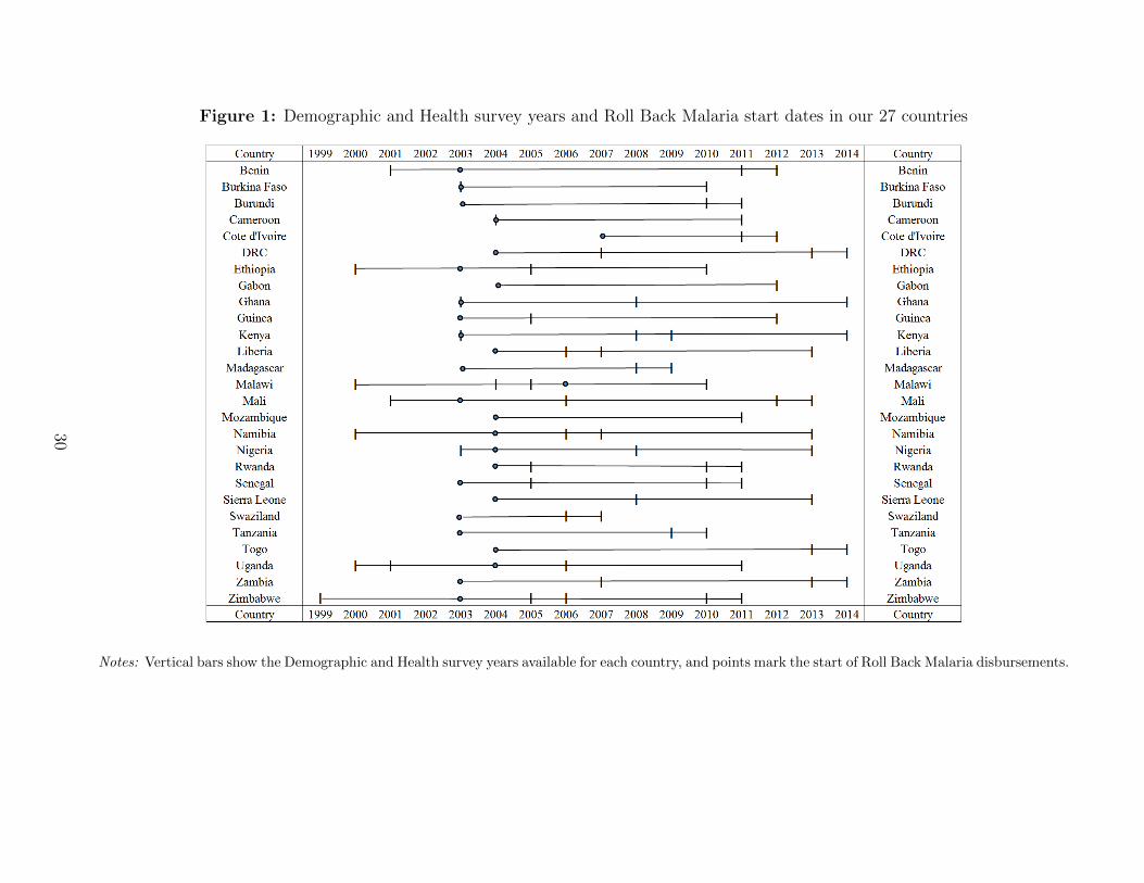
Figure 1: Demographic and Health survey years and Roll Back Malaria start dates in our 27 countries

Notes: Vertical bars show the Demographic and Health survey years available for each country, and points mark the start of Roll Back Malaria disbursements.

30

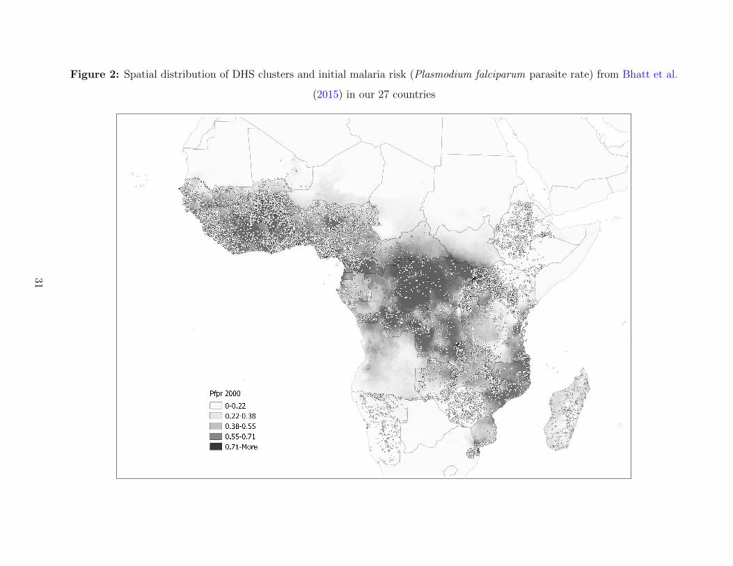
Figure 2: Spatial distribution of DHS clusters and initial malaria risk (Plasmodium falciparum parasite rate) from Bhatt et al.

(2015) in our 27 countries

31

Figure 3: Evolution of malaria risk (Plasmodium falciparum parasite rate) and coverage

by malaria control strategies in our 27 sample countries

Notes: Each line plots annualized indicators from the Malaria Atlas Project, totaled for all countries in

our sample, over time. The vertical bar denotes the scale-up of RBM disbursements. Figure 3a plots the

mean malaria risk (Plasmodium falciparum parasite rate). Figure 3b plots the mean coverage of artemisinin

combination therapies. Figure 3c plots the mean coverage of insecticide treated nets. Figure 3d plots the

mean coverage of indoor residual spraying.

32

Figure 4: Evolution of regional malaria risk conditional on initial malaria risk (Plasmodium falciparum parasite rate)

Notes: Each point represents a region. We obtain yearly malaria risk (PfPR) from the Malaria Atlas Project. In a univariate regression of the change in

malaria risk between 2003 and 2005, the coefficient of initial malaria risk is -0.064 and is statistically significant at 0.1% (Figure 4b, N = 155).

33

Figure 5: Evolution of bednets and antimalarial use conditional on initial malaria risk (Plasmodium

falciparum parasite rate)

Notes: Each point represents a region. We obtain yearly malaria risk from the Malaria Atlas Project. The

change in Figures 5a, 5c, and 5d is the difference between the first and last DHS survey available in our

sample. The change in Figure 5b is the difference between 2003 and 2015, the latest available year of MAP

data. In a univariate regression of the change in household bednet use for children under 5 (from the DHS)

on initial malaria risk (in 2000), the coefficient of initial malaria risk is 0.148 and is statistically significant

at the 10% level (Figure 5a, N = 108). For the change in bednet use (from the Malaria Atlas Project), the

coefficient of initial malaria risk is 0.586 and is statistically significant at the 0.1% level (Figure 5b, N =

155). For the change in chloroquine use for fever in children under 5, the coefficient of initial malaria risk

is -0.554 and is statistically significant at the 0.1% level (Figure 5c, N = 39). For the change in artemisinin

combination therapy use for fever in children under 5, the coefficient of initial malaria risk is 0.074 but it is

not statistically significant due to the low number of observations (Figure 5d, N = 32).

34

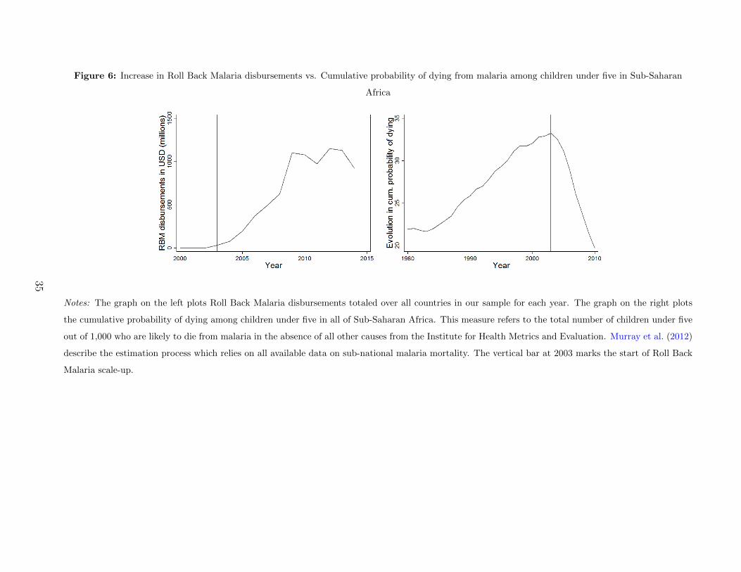
Figure 6: Increase in Roll Back Malaria disbursements vs. Cumulative probability of dying from malaria among children under five in Sub-Saharan

Africa

Notes: The graph on the left plots Roll Back Malaria disbursements totaled over all countries in our sample for each year. The graph on the right plots

the cumulative probability of dying among children under five in all of Sub-Saharan Africa. This measure refers to the total number of children under five

out of 1,000 who are likely to die from malaria in the absence of all other causes from the Institute for Health Metrics and Evaluation. Murray et al. (2012)

describe the estimation process which relies on all available data on sub-national malaria mortality. The vertical bar at 2003 marks the start of Roll Back

Malaria scale-up.

35

Figure 7: Relationship of initial malaria risk with infant mortality, fertility, adult labor supply and

education

Notes: These graphs display the standardized relationship of pre-campaign malaria risk with each outcome

variable by cohort. For each cohort, we regress of the standard deviation of the dependent variable on the

standard deviation of malaria risk in 2000, controlling for individual covariates and survey year.

36

Table 1: Ruling out pre-campaign catch-up effects

Coefficient of (malaria2000j × exposureNct)

Dep. var. (1) (2) (3)

Height-For-Age z-scores -8.202 -19.649 -26.920

(50.291) (62.725) (74.468)

R2 0.257 0.258 0.259

Observations 276,860 276,860 276,860

Years of education completed -2.929ˆ -4.235* -4.189ˆ

(1.546) (1.929) (2.227)

R2 0.565 0.566 0.566

Observations 565,214 565,214 565,214

Primary education completed -0.161 -0.262 -0.488*

(0.168) (0.207) (0.239)

R2 0.476 0.476 0.477

Observations 565,214 565,214 565,214

Age-by-region FE no yes yes

Exposure-by-region FE no no yes

Notes: The unit of observation is the individual. For all dependent variables

listed on the left, each cell reports the OLS estimate of coefficient β in Equa-

tion (1). The regression controls for gender, wealth, and DHS cluster fixed

effects as well as country-by-cohort-by-DHS year fixed effects and their sub-

components. Standard errors (in parentheses) are clustered at the DHS cluster

level. ˆ, *, ** and *** indicate significance at the 10, 5, 1 and 0.1% levels.

37

Table 2: Difference in means analysis of human capital outcomes

Dep. var. (1) (2) (3) Dep. var. (1) (2) (3)

Post-RBM Pre-RBM Difference Post-RBM Pre-RBM Difference

Infant mortality Employed in last 12 mo. (adult)

Highly malarious 0.066 1.000 -0.034*** Highly malarious 0.706 0.649 0.057***

Less malarious 0.063 0.089 -0.026*** Less malarious 0.671 0.631 0.040***

-0.008*** 0.017***

Neonatal mortality Paid in cash when emp. (adult)

Highly malarious 0.033 0.047 -0.014*** Highly malarious 0.647 0.578 0.069***

Less malarious 0.033 0.043 -0.010*** Less malarious 0.719 0.715 0.004

-0.004*** 0.065***

Postnatal mortality Years of ed.

Highly malarious 0.035 0.058 -0.023*** Highly malarious 3.038 2.014 1.024***

Less malarious 0.032 0.050 -0.018*** Less malarious 3.559 2.915 0.644***

-0.005*** 0.380***

Tot. births Completed primary ed.

Highly malarious 2.935 2.637 0.299*** Highly malarious 0.245 0.138 0.107***

Less malarious 2.647 2.254 0.394*** Less malarious 0.296 0.227 0.069***

-0.095*** 0.380***

Notes: A highly (resp. less) malarious DHS cluster is defined as having an above (resp. below) median level of malaria risk in 2000.

Pre-campaign surveys occur prior to 2003 and post-campaign surveys occur in 2003 or later.

38

Table 3: Effect of the RBM campaign on human capital outcomes

Coefficient of (malaria2000j × exposureNct)

(1) (2) (3) (4) (5) (6)

Infant Neonatal Postnatal

-0.514*** -0.182*** -0.458*** -0.140* -0.546*** -0.135*

(0.040) (0.050) (0.049) (0.051) (0.055) (0.053)

R2 0.126 0.323 0.117 0.323 0.126 0.320

Observations 341,542 341,542 329,786 329,786 330,171 330,171

Exposure-by-region FE no yes no yes no yes

Tot. births

-3.951*** -3.242*** -3.837***

(0.213) (0.241) (0.291)

R2 0.659 0.665 0.666

Observations 646,169 646,169 646,169

Age-by-region FE no yes yes

Exposure-by-region FE no no yes

Employed last 12 mo. (adult) Paid in cash for emp. (adult)

0.361*** 0.316*** 0.489*** 0.215*** 0.181* 0.175*

(0.040) (0.048) (0.057) (0.049) (0.059) (0.068)

R2 0.328 0.333 0.334 0.409 0.411 0.412

Observations 896,857 896,857 896,857 607,572 607,572 607,572

Age-by-region FE no yes yes no yes yes

Exposure-by-region FE no no yes no no yes

Years of ed. Completed primary ed.

1.913*** 1.776*** 2.406*** 0.178*** 0.167*** 0.224***

(0.087) (0.082) (0.112) (0.008) (0.008) (0.011)

R2 0.614 0.632 0.634 0.521 0.535 0.537

Observations 2,841,538 2,841,538 2,841,538 2,841,538 2,841,538 2,841,538

Age-by-region FE no yes yes no yes yes

Exposure-by-region FE no no yes no no yes

Notes: The unit of observation is the individual. For all dependent variables, each cell reports

the OLS estimate of coefficient β in Equation (1). The regression controls for gender, wealth, and

DHS cluster fixed effects as well as country-by-cohort-by-DHS year fixed effects and their subcom-

ponents. Standard errors (in parentheses) are clustered at the DHS cluster level. ˆ, *, ** and ***

indicate significance at the 10, 5, 1 and 0.1% levels.

39

Table 4: Controlling for exposure to concurrent public policies interacted with malaria risk in 2000 in baseline equation

Coefficient of (malaria2000j × exposure)

(1) (2) (3) (4) (5) (6) (7) (8)

Infant Neonatal Postnatal Tot. births Employed Paid in cash Years of ed. Completed primary ed.

Education -0.082ˆ -0.037 -0.085ˆ -2.940*** 0.300*** 0.207* 1.937*** 0.178***

(0.045) (0.045) (0.048) (0.350) (0.070) (0.082) (0.121) (0.012)

R2 0.551 0.553 0.546 0.667 0.335 0.413 0.634 0.538

Observations 341,542 329,786 330,171 646,169 896,857 607,572 2,841,538 2,841,538

Health -0.092* -0.044 -0.093* -3.408*** 0.364*** 0.200* 1.992*** 0.192***

(0.034) (0.034) (0.035) (0.407) (0.084) (0.101) (0.134) (0.013)

R2 0.637 0.649 0.623 0.667 0.335 0.413 0.635 0.538

Observations 341,542 329,786 330,171 646,169 896,857 607,572 2,841,538 2,841,538

Military -0.059ˆ -0.031 -0.055 -3.191*** 0.350*** 0.265* 2.040*** 0.188***

(0.034) (0.033) (0.037) (0.346) (0.071) (0.086) (0.112) (0.011)

R2 0.636 0.643 0.629 0.667 0.335 0.413 0.634 0.538

Observations 341,542 329,786 330,171 646,169 896,857 607,572 2,841,538 2,841,538

All Govt. -0.387*** -0.350*** -0.395*** -2.514*** 0.189* 0.056 1.421*** 0.143***

(0.024) (0.033) (0.029) (0.439) (0.091) (0.106) (0.104) (0.010)

R2 0.615 0.618 0.605 0.666 0.334 0.412 0.634 0.538

Observations 341,542 329,786 330,171 646,169 896,857 607,572 2,841,538 2,841,538

FPE -2.093*** 0.532*** 0.181ˆ 1.911*** 0.190***

(0.415) (0.087) (0.104) (0.137) (0.013)

R2 0.667 0.335 0.413 0.635 0.539

Observations 646,169 896,857 607,572 2,841,538 2,841,538

Notes: The unit of observation is the individual. For all dependent variables, each cell reports the OLS estimate of coefficient β in

Equation (1). The regression controls for gender and wealth as well as fixed effects for DHS clusters, country-by-cohort-by-DHS year

and subcomponents, age-by-region, and exposure-by-region. Standard errors (in parentheses) are clustered at the DHS cluster level. ˆ,

*, ** and *** indicate significance at the 10, 5, 1 and 0.1% levels.

40

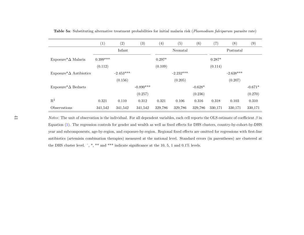
Table 5a: Substituting alternative treatment probabilities for initial malaria risk (Plasmodium falciparum parasite rate)

(1) (2) (3) (4) (5) (6) (7) (8) (9)

Infant Neonatal Postnatal

Exposure*∆ Malaria 0.399*** 0.297* 0.287*

(0.112) (0.109) (0.114)

Exposure*∆ Antibiotics -2.453*** -2.232*** -2.638***

(0.156) (0.205) (0.207)

Exposure*∆ Bednets -0.890*** -0.628* -0.671*

(0.257) (0.236) (0.270)

R2 0.321 0.110 0.312 0.321 0.106 0.316 0.318 0.103 0.310

Observations 341,542 341,542 341,542 329,786 329,786 329,786 330,171 330,171 330,171

Notes: The unit of observation is the individual. For all dependent variables, each cell reports the OLS estimate of coefficient β in

Equation (1). The regression controls for gender and wealth as well as fixed effects for DHS clusters, country-by-cohort-by-DHS

year and subcomponents, age-by-region, and exposure-by-region. Regional fixed effects are omitted for regressions with first-line

antibiotics (artemisin combination therapies) measured at the national level. Standard errors (in parentheses) are clustered at

the DHS cluster level. ˆ, *, ** and *** indicate significance at the 10, 5, 1 and 0.1% levels.

41

Table 5b: Substituting alternative treatment probabilities for initial malaria risk (Plasmodium falciparum

parasite rate)

(1) (2) (3) (4) (5) (6)

Tot. births

Exposure*∆ Malaria 8.056***

(0.640)

Exposure*∆ Antibiotics -72.663***

(5.507)

Exposure*∆ Bednets -9.945***

(0.826)

R2 0.666 0.651 0.665

Observations 646,169 646,169 646,169

Employed last 12 mo. Paid in cash for emp.

Exposure*∆ Malaria -1.027*** -0.357*

(0.123) (0.140)

Exposure*∆ Antibiotics 6.837*** 3.797***

(0.858) (0.891)

Exposure*∆ Bednets 1.302*** 0.412*

(0.158) (0.161)

R2 0.334 0.325 0.333 0.412 0.409 0.412

Observations 896,857 896,857 896,857 607,572 607,572 607,572

Years of ed. Completed primary ed.

Exposure*∆ Malaria -4.717*** -0.440***

(0.247) (0.024)

Exposure*∆ Antibiotics 36.127*** 3.370***

(2.531) (0.239)

Exposure*∆ Bednets 7.304*** 0.681***

(0.399) (0.039)

R2 0.630 0.596 0.630 0.534 0.507 0.534

Observations 2,841,538 2,841,538 2,841,538 2,841,538 2,841,538 2,841,538

Notes: The unit of observation is the individual. For all dependent variables, each cell reports the

OLS estimate of coefficient β in Equation (1). The regression controls for gender and wealth as well

as fixed effects for DHS clusters, country-by-cohort-by-DHS year and subcomponents, age-by-region,

and exposure-by-region. Standard errors (in parentheses) are clustered at the DHS cluster level. ˆ,

*, ** and *** indicate significance at the 10, 5, 1 and 0.1% levels.

42

Table 6: Estimating baseline equation with restricted sub-samples

(1) (2) (3) (4) (5) (6) (7) (8)

Infant Neonatal Postnatal Tot. births Employed Paid in cash Years of ed. Completed primary ed.

Residentsa -0.090 -0.150 -0.021 -2.977*** 0.594*** -0.122 1.556*** 0.152***

(0.117) (0.115) (0.117) (0.824) (0.118) (0.177) (0.231) (0.027)

R2 0.647 0.656 0.643 0.703 0.396 0.442 0.667 0.550

Observations 55,849 53,604 53,804 100,647 174,562 122,643 430,696 430696

Born before 1960 -3.825*** 0.476*** 0.179* 2.263*** 0.206***

(0.291) (0.056) (0.067) (0.104) (0.010)

R2 0.668 0.334 0.413 0.604 0.512

Observations 670,113 950,792 651,475 3,235,297 3,235,297

Above age 5 -3.837*** 0.489*** 0.175* 3.140*** 0.293***

(0.291) (0.057) (0.068) (0.169) (0.017)

R2 0.666 0.334 0.412 0.597 0.512

Observations 646,169 896,857 607,572 2,313,954 2,313,954

Notes: The unit of observation is the individual. For all dependent variables, each cell reports the OLS estimate of coefficient β in Equa-

tion (1). The regression controls for gender, wealth, and DHS cluster fixed effects as well as country-by-cohort-by-DHS year fixed effects

and their subcomponents. Standard errors (in parentheses) are clustered at the DHS cluster level. ˆ, *, ** and *** indicate significance

at the 10, 5, 1 and 0.1% levels.

a When we drop exposure-by-region fixed effects (a demanding control given the small sample size), we obtain the following coefficients

and standard errors: infant (-2.806*** [0.080]), neonatal (-2.710*** [0.096]), postnatal (-2.502*** [0.087]).

43

FOR ONLINE PUBLICATION

Supplemental Appendix to Disease and Human

Capital Accumulation: Evidence from the Roll Back

Malaria Partnership in Africa

1 Model

1.1 Set-up

We consider a unitary household composed of one adult and her potential surviving off-

spring.1 We assume that the household cares about its own consumption c and leisure `

as well as about the number n and human capital h of the offspring. Though human cap-

ital in childhood is an important determinant of future earnings (Becker, 1975; Currie and

Madrian, 1999; Currie, 2009; Hong, 2013), we focus only on contemporaneous effects of im-

proved health on fertility, labor supply and education. We denote by b the number of births

and by s the probability for a newborn to survive, such that n = sb (with 0 < s < 1).

The household’s preferences are summarized by the following Cobb-Douglas utility function:

u(c, `, sb, h(e,H)) = (c`)1−γ(sbh(e,H))γ, (1)

where

0 < γ < 1 and h(e,H) = (eρ +Hρ)1ρ with ρ < 1.

1The impact of children’s exposure to malaria control campaigns on their adult longevity has not yetbeen documented (and cannot be investigated based on our data). Our analysis therefore relies on a one-period model, with no reference to adult longevity. The interplay between adult longevity and some of ouroutcomes is complex. For instance, increased longevity does not necessarily increase parents’ incentives toinvest in their offspring’s education. On one hand, the longer the stream of payouts, the more valuablethe investment. Increased longevity should therefore translate into more parental investment in education(Ben-Porath, 1967; Soares, 2005; Jayachandran and Lleras-Muney, 2009). On the other hand however, ahigher life expectancy affects not only the returns to children’s quality but also the returns to their quantity.Greater longevity might therefore result in no increase in the level of education chosen by the parents (Hazanand Zoabi, 2006) and could even reduce income per capita (Acemoglu and Johnson, 2007). As is apparentfrom the subsequent sections, the impact of improved children’s survival rate and health on our variousoutcomes is not trivial either.

1

The human capital h(e,H) of a surviving child is assumed to be a CES production function

that depends on his/her education e and his/her health H, with H > 1. We denote by σ the

elasticity of substitution between these two inputs. Therefore, σ = 11−ρ . The lower (resp.

the higher) ρ, the higher the complementarity (resp. the substitutability).2 In particular, if

ρ < 0, then the impact of one additional unit of education on human capital increases with

health (heH > 0). If 0 < ρ < 1 instead, the reverse is true (heH < 0).

For the sake of generality, we allow ρ to take positive values. We assume that each member

of the household is endowed with one unit of time. The adult allocates this unit between

work, leisure and the time she spends on caring for her surviving child(ren). We denote by

τ the time the parent dedicates to each surviving child, with τ > 0.3 As for each surviving

child, she allocates her unit of time between education and child labor. Put differently, we

assume that education and child labor are mutually exclusive.4 The wage rates of the parent

and of each child are denoted by W and w(H) = wH respectively, with W > 0 and w > 0.5

Therefore, the budget constraint is

c ≤ W (1− `− τsb) + sbwH(1− e). (2)

The parameters of the model are chosen to yield an interior solution for the optimal number

of births b∗, the optimal level of leisure `∗ and the optimal level of education e∗. More

precisely, they ensure that (i) 0 < b∗ < W (1−`∗)s(Wτ−wH(1−e∗)) , that (ii) 0 < `∗ < 1 (iii) and that

0 < e∗ < 1. The first condition is obtained by assuming a positive consumption. This

notably implies that Wτ − wH(1 − e∗) > 0 for all e∗ between 0 and 1. Put differently, a

surviving child must cost more than the labor earnings she generates. Otherwise, the optimal

number of births is infinite.

2If ρ converges to 1, h(e,H) is a linear production function; if ρ converges to 0, h(e,H) is a Cobb-Douglasproduction function; if ρ converges to −∞, h(e,H) is a Leontief production function.

3For the sake of simplicity, but without loss of generality, τ depends on neither e nor H.4Evidence confirms that, on average, child labor and education exert a negative impact on one another

(Beegle, Dehejia and Gatti, 2009; Edmonds and Shrestha, 2014), although exceptions obviously exist (Basuand Van, 1998; Basu, 1999; Psacharopoulos, 1997).

5Just as w(H) depends positively on H, W depends positively on the parent’s health. However, thisrelationship is not made explicit since we focus on the impact of an increase in children’s survival rate andhealth.

2

1.2 Predictions

Solving the model yields the optimal level of education e∗, the optimal amount of time

worked by the parent Λ∗ and the optimal number of births b∗:

e∗ = (Wτ − wHwHρ+1

)

11−ρ

, (3)

Λ∗ = 1− `∗ − τsb∗ =(1− γ)Wτ − wH(1− e∗)

(2− γ)(Wτ − wH(1− e∗)), (4)

and

b∗ =γW

(2− γ)s(Wτ − wH(1− e∗)). (5)

Proof :

Using monotonic transformation, the household’s preferences can be represented by

U(c, `, sb, h(e,H)) = (1− γ)[log c+ log `] + γ[log sb+ log h(e,H)],

which yields the following maximization problem:

maxe,b,`

(1− γ)[log(W (1− `− τsb) + w(H)sb(1− e)) + log `] + γ[log sb+ log h(e,H)].

The first-order conditions for the optimal level of education e∗, for the optimal number of

births b∗ and for the optimal level of leisure `∗ are given by Equations (1) to (3) respectively:

γeρ−1

eρ +Hρ=

(1− γ)sbwH

W (1− `)− sb(Wτ − wH(1− e)), (6)

γ

b=

(1− γ)s(Wτ − wH(1− e))W (1− `)− sb(Wτ − wH(1− e))

, (7)

and

1

`=

W

W (1− `)− sb(Wτ − wH(1− e)). (8)

Dividing Equation (1) by Equation (2) and rearranging yields

3

e∗ = (Wτ − wHwHρ+1

)

11−ρ

.

Solving the system of Equation (2) and Equation (3) yields

`∗ =1− γ2− γ

,

and

b∗ =γW

(2− γ)s(Wτ − wH(1− e∗))

�

We observe that b∗ declines in inverse proportion to the survival rate s. Indeed, since parents

care about surviving children, this probability affects parents’ fertility choices through the

net cost of a surviving child (denoted by Wτ − wH(1 − e∗)), which is independent of s.

Consequently, parents choose the preferred number of surviving children irrespective of s,

leading to a total number of births that is inversely proportional to this parameter. Therefore,

since education and labor supply depend on the number of surviving children (not on the

total number of births), they are not affected by s.

1.2.1 The optimal level of education

The optimal level of education e∗ increases with child health if ρ < ρ1, with ρ1 = − WτWτ−wH ;

e∗ decreases with child health otherwise.

Proof :

Deriving e∗ with respect to H yields

∂e∗

∂H= −(

1

1− ρ)(ρ(Wτ − wH) +Wτ

wHρ+2)(Wτ − wHwHρ+1

)

ρ1−ρ

.

We observe that ∂e∗

∂His of the opposite sign of ρ(Wτ − wH) + Wτ . More precisely, ∂e∗

∂His

positive if ρ < − WτWτ−wH . It is negative otherwise. �

4

Consistent with Bleakley (2010), an increase in child health raises their wage rate (wH) and,

hence, the opportunity cost of education. If education and health are substitutes (0 < ρ < 1),

this negative effect is reinforced. If, however, education and health are complements (ρ < 0),

an increase in health generates an additional impact that runs in the opposite direction:

better health improves the returns to education. In this setting, if the complementarity

between education and health is sufficiently high (ρ < ρ1), then the latter effect wins out,

and e∗ increases with child health.

1.2.2 The optimal labor supply and number of births

The optimal labor supply Λ∗ increases with child health while the optimal number of births

b∗ decreases with child health if ρ < ρ2, with ρ2 < ρ1; Λ∗ (resp. b∗) decreases (resp. increases)

with child health otherwise.

Proof :

Deriving Λ∗ and b∗ with respect to H yields

∂Λ∗

∂H= −

γWτw(1− e∗ − ∂e∗

∂HH)

(2− γ)(Wτ − wH(1− e∗))2,

and

∂b∗

∂H=

γWw(1− e∗ − ∂e∗

∂HH)

(2− γ)s(Wτ − wH(1− e∗))2

respectively.

We observe that Λ∗ (resp. b∗) increases (resp. decreases) with H when ∂e∗

∂H> 1−e∗

H> 0.

Yet, as we show below, ∂e∗

∂Hdecreases with ρ when it is positive. Consequently, there exists

a unique value of ρ, that we denote by ρ2, such that (i) ∂e∗

∂H= 1−e∗

H; (ii) ∂e∗

∂H> 1−e∗

Hwhen

ρ < ρ2; (iii) ∂e∗

∂H< 1−e∗

Hwhen ρ > ρ2. Given that 1−e∗

His strictly positive, ρ2 is necessarily

lower than ρ1 = − WτWτ−wH .

To show that ∂e∗

∂Hdecreases with ρ when it is positive, one can rewrite ∂e∗

∂Has the product of

two functions, denoted byf(ρ) and g(ρ), with

5

f(ρ) = −wH(ρ(Wτ − wH) +Wτ)

1− ρ

and

g(ρ) = (Wτ − wHwH2

)

ρ1−ρ

.

When ∂e∗

∂His positive (i.e. ρ < − Wτ

Wτ−wH ), f(ρ) is a positive decreasing function of ρ. More-

over, using the fact that e∗ must be comprised between 0 and 1 and, hence, that Wτ−wHwHρ+1 < 1

for ρ < 1, it is easy to show that g(ρ) is also a positive decreasing function of ρ. Therefore,

∂e∗

∂His decreasing with ρ when it is positive. �

We know that an increase in child health decreases each child’s “price” by raising their wage

rate wH. As a result, the adult’s labor supply decreases, and her preferred number of births

increases. If education also decreases with health, these effects are reinforced since better

health increases children’s working time. If, however, education increases with health, then a

child’s “price” increases. Provided that the complementarity between education and health

is sufficiently high, this counter-effect wins out: the parent’s labor supply increases and her

preferred number of births decreases, following a well-documented quality-quantity trade-off

(Becker and Lewis, 1973; Rosenzweig and Zhang, 2009; Bleakley and Lange, 2009).6

Note that the condition of ρ2 < ρ1, emphasized in Proposition 3, is more binding than that of

Proposition 2. For the labor supply (resp. the number of births) to increase (resp. decrease)

with health, the impact of health on education does not simply need to be positive: it must

be greater than a strictly positive value.

2 Data

Human capital

Source(s): The Demographic and Health Surveys are nationally representative studies

that collect detailed information on numerous population and health characteristics. We

select 27 countries which were surveyed at least once post-campaign, which received RBM

6The variation in opposite directions of Λ∗ and b∗ is intuitive: a lower fertility allows the parent todedicate more time to the labor market, while a lower labor supply allows the parent to raise more children.

6

disbursements, and which include geocoded clusters and all of our outcome variables. Figure

1 outlines the period of time covered for each country within the range of 1999 to 2014.

Infant mortality (infants): Because infant mortality may vary substantially within the

first year of life, we follow Pathania (2014) to compute three binary indicators of mortality:

neonatal (if death occurred within the first month of life); postnatal (if death occurred within

months 1-11); infant (if death occurred within first year of life) from the Child Recode of

children under five.

Total births (women): Total number of children ever born to eligible women (ages 15 to

45) in the Individual Recode.

Total years of education (all): Education in single years for all individuals in the DHS

Person Recode.

Completed primary education (all): We use total years of education to compute an

indicator for all respondents who have completed at least the full number of years of primary

education (5, 6 or 7) in their country’s educational system.

Employed in last 12 mo. (adults): Binary variable equal to one if respondent was

employed within last 12 months for all eligible respondents in Individual and Male Recodes.

Paid in cash for employment (adults): Binary variable equal to one if respondent is

paid at least partly in cash while employed for all eligible respondents in Individual and

Male Recodes.

Hours worked (children): A subset of DHS surveys contain child labor modules (Benin,

Burkina Faso, Burundi, Cote d’Ivoire, DRC, Cameroon, Gabon, Guinea, Mali, Malawi,

Rwanda, Sierra Leone, Senegal, Togo, and Uganda). From these surveys, we rely on the

number of hours worked by a child (ages 5 to 14) over the previous week.

RBM disbursements

Source(s): According to Pigott et al. (2012), the three largest funders of anti-malaria

campaigns to date, aside from governments, are the Global Fund to Fight AIDS, Tuberculosis

and Malaria (since 2003), the President’s Malaria Initiative (since 2005), and the World Bank

Booster Program for Malaria Control in Africa (since 2006). We focus on external aid, using

fixed effects and robustness checks to address the question of malaria-specific government

expenditure. We extract GFATM disbursements on malaria, tuberculosis, and HIV/AIDS by

7

year from individual country files available at the International Aid Transparency Initiative

website (http://iatiregistry.org/). We transcribe PMI expenditures by country and

year from the PMI Ninth Annual Report to Congress (2005-2014). Finally, we rely on data

kindly provided by David Pigott to compile disbursements from the World Bank Booster

Program. We total RBM disbursements by country and year following studies on malaria

expenditure (Snow et al., 2010; Pigott et al., 2012). Because these disbursements are at the

country-year level, we merge them with each DHS recode by country-year. In a handful

of cases, negative disbursements indicate corrupt or inefficient use of funds that donors

requested for return.

Exposure to RBM campaigns: Exposure captures the yearly amount per capita (at the

country level)7 disbursed by the three main RBM funders during a respondent’s lifetime.

A respondent’s lifetime is defined as the difference between the DHS survey year and this

individual’s year of birth, from which we subtract one year. We consider a respondent’s

exposure to begin in utero (though defining the beginning as the year after birth does not

alter our results). To illustrate the construction of this variable, we take the example of

Ethiopia. As reported in Figure 1, RBM campaigns in Ethiopia started in 2003. Moreover,

three DHS surveys years are available (in 2000, 2005 and 2010). Let’s consider an individual

born in 1999. If this individual is surveyed in 2000, he experiences no exposure since the RBM

disbursements were to begin only in 2003. If he is surveyed instead in 2005, he experiences

three years of exposure to RBM disbursements. His exposure will therefore be equal to the

sum of the RBM disbursements per capita during these three years, divided by his lifetime,

hence 2005-(1999-1)=7 years. Similarly, if this individual is surveyed in 2010, he experiences

eight years of exposure to RBM disbursements. His exposure will therefore be equal to the

sum of RBM disbursements per capita during these eight years, divided by his lifetime, hence

2010-(1999-1)=12 years.

Malaria risk and control programs

Source(s): We obtain data on malaria prevalence and control strategies from the Malaria

Atlas Project (http://www.map.ox.ac.uk/). Data on ITN use and access to ACTs from

over one million households were combined with national malaria control programme data

7Yearly population data come from the World Development Indicators.

8

on ITN, ACT and IRS provision to develop time-series models of coverage at the country

level (Bhatt et al., 2015). We use the DHS to provide complementary measures of control

strategies from microdata.

Malaria risk (2000-2015): We proxy for malaria risk by relying on the P. falciparum

parasite rate (PfPR) computed for each DHS cluster. For a given year, PfPR describes

the estimated proportion of individuals in the general population aged 2 to 10 years old

who are infected with P. falciparum at any given time. These estimates are generated

by a geostatistical model that relies on parasite rate surveys as well as bioclimatic and

environmental characteristics. Gething et al. (2011) and Bhatt et al. (2015) describe the

estimation process.

Insecticide treated net coverage (MAP): Calculated at the household level as the

proportion of individuals who slept under a net.

Artemisin combination therapies coverage (MAP): Percentage of fever cases in chil-

dren under five treated with ACT.

Indoor residual spraying coverage (MAP): Proportion of the population at risk of

malaria who benefits from IRS.

Insecticide treated net usage (DHS): Proportion of households per region that always

use ITN for children under 5 (DHS Household Recode).

Artemisin combination therapies usage (DHS): Proportion of children under five per

region treated for fever with ACT during past 2 weeks (DHS Child Recode).

Chloroquine usage (DHS): Proportion of children under five per region treated for fever

with chloroquine during past 2 weeks (DHS Child Recode).

Public expenditure

We obtain expenditure on public education as a percentage of GDP from the World Bank

EdStats, Education Statistics: Core Indicators. To compute total public expenditure per

capita in each of these categories, we rely on GDP in current USD and total population

(both from WDI).

9

3 Tables

Table A1: Descriptive statistics

Mean SD Min Max N

(1) (2) (3) (4) (5)

Explanatory variables

Malaria risk (PfPR in 2000) 0.351 0.236 0.000 0.964 25,827

Exposure to Roll Back Malaria 0.570 0.787 -0.162 8.918 2,857,253

Dependent variables

Child survival and health

Infant mortality 0.068 0.251 0 1 341,829

Neonatal mortality 0.034 0.182 0 1 330,094

Postnatal mortality 0.036 0.185 0 1 330,475

Fertility

Total number of births 2.757 2.722 0 18 646,208

Adult labor supply

Employed in last 12 months 0.684 0.465 0 1 896,887

Paid in cash if employed 0.680 0.466 0 1 607,668

Education

Number of years of education completed 3.220 4.137 0 26 2,850,793

Primary education completed 0.262 0.440 0 1 2,850,793

Socioeconomic controls

Male 0.489 0.500 0 1 2,866,372

Age 16.837 12.930 0 53 2,866,431

Wealth 2.969 1.427 1 5 2,866,431

Notes : The variables are measured at the individual level, with the exception of PfPR

in 2000 which is computed at the DHS cluster level.

10

Table A2: Descriptive statistics for exposure to Roll Back Malaria disbursements

Date of birth Mean SD Min Max N Age Mean SD Min Max N

(1) (2) (3) (4) (5) (6) (7) (8) (9) (10)

1965 0.119 0.148 0.000 0.705 25,475 0 1.190 1.093 -0.162 4.251 112,882

1970 0.130 0.160 0.000 0.785 32,186 5 1.007 1.044 0.000 5.024 95,621

1975 0.154 0.185 0.000 0.885 39,127 10 0.604 0.655 0.000 3.139 107,579

1980 0.176 0.210 0.000 1.016 46,755 15 0.409 0.455 0.000 2.158 70,563

1985 0.211 0.250 0.000 1.191 54,222 20 0.293 0.336 0.000 1.644 70,973

1990 0.243 0.298 0.000 1.439 63,871 25 0.236 0.268 0.000 1.328 63,667

1995 0.331 0.377 0.000 1.817 77,621 30 0.202 0.225 0.000 1.114 63,188

2000 0.522 0.526 0.000 2.466 101,094 35 0.178 0.196 0.000 0.959 51,359

2005 1.108 0.768 0.000 3.793 88,740 40 0.162 0.174 0.000 0.842 43,139

2010 1.993 1.252 0.132 6.822 57,944 45 0.181 0.153 0.010 0.751 25,535

2014 1.498 0.558 0.000 1.835 8,280 50 0.246 0.152 0.091 0.677 12,095

Survey year Survey year

1999 0.000 0.000 0.000 0.000 22,263 2007 0.391 0.505 0.016 3.263 130,321

2000 0.000 0.000 0.000 0.000 148,225 2008 0.219 0.242 0.026 1.604 242,097

2001 0.000 0.000 0.000 0.000 94,699 2009 0.563 0.430 0.108 2.287 81,118

2002 . . . . . 2010 0.786 0.741 0.087 4.566 385,477

2003 0.005 0.008 0.000 0.050 133,568 2011 0.868 0.774 0.091 4.199 258,130

2004 0.008 0.018 0.000 0.107 83,450 2012 0.949 0.811 -0.162 3.519 219,140

2005 0.096 0.140 0.000 0.944 226,954 2013 1.026 1.171 0.000 8.918 453,016

2006 0.159 0.238 0.010 1.760 136,707 2014 0.971 0.609 0.000 2.598 251,266

Country Country

Benin 1.145 1.063 0.000 4.067 105,223 Mali 0.334 0.578 0.000 2.539 170,726

Burkina Faso 0.380 0.622 0.001 3.128 118,737 Mozambique 0.770 0.532 0.167 2.024 56,122

Burundi 0.517 0.371 0.116 1.676 38,501 Nambia 1.078 1.642 0.000 8.918 97,664

DRC 0.515 0.509 0.016 1.830 123,167 Nigeria 0.272 0.258 0.000 0.891 325,292

Cote d’Ivoire 0.476 0.373 0.091 1.794 44,616 Rwanda 1.058 1.227 0.028 4.566 92,345

Cameroon 0.362 0.603 0.002 3.381 107,951 Senegal 0.648 0.707 0.024 2.504 123,800

Ethiopia 0.170 0.256 0.000 1.238 178,991 Sierra Leone 0.451 0.346 0.046 1.467 103,122

Gabon 0.605 0.402 -0.162 1.387 34,729 Swaziland 0.089 0.076 0.020 0.352 18,776

Ghana 0.570 0.662 0.001 2.502 98,760 Tanzania 0.930 0.710 0.154 2.416 42,984

Guinea 0.396 0.541 0.011 2.630 70,528 Togo 0.493 0.315 0.000 1.154 42,056

Kenya 0.689 0.540 0.001 1.835 204,828 Uganda 0.432 0.490 0.000 1.740 107,516

Liberia 1.771 1.654 0.080 5.294 73,229 Zambia 1.335 0.889 0.130 3.670 108,573

Madagascar 0.540 0.419 0.096 1.604 75,111 Zimbabwe 0.184 0.298 0.000 1.588 94,030

Malawi 0.440 0.631 0.000 2.164 209,054

11

Table A3: Correlation of children’s survival rate and health, fertility, adult labor market outcomes and education with variations

in malaria prevalence, malaria incidence and coverage by antimalarial strategies

(1) (2) (3) (4) (5) (6) (7) (8)

∆ Risk ∆ Incid. ∆ Drugs (MAP) ∆ Drugs (DHS) ∆ Nets (MAP) ∆ Nets (DHS) ∆ Under 5 nets (DHS) ∆ Spraying (MAP)

Infant 0.053*** 0.077*** -0.033*** -0.194*** -0.037*** -0.046*** -0.050*** -0.086***

(0.003) (0.003) (0.003) (0.009) (0.002) (0.002) (0.003) (0.004)

R2 0.333 0.333 0.332 0.414 0.333 0.358 0.353 0.333

Observations 341,829 341,829 341,829 129,220 341,829 191,182 142,846 341,829

Neonatal 0.025*** 0.037*** -0.017*** -0.112*** -0.018*** -0.024*** -0.025*** -0.047***

(0.002) (0.003) (0.003) (0.007) (0.001) (0.002) (0.003) (0.003)

R2 0.202 0.202 0.202 0.259 0.202 0.220 0.220 0.203

Observations 330,094 330,094 330,094 122,932 330,094 184,256 137,826 330,094

Postnatal 0.042*** 0.060*** -0.025*** -0.148*** -0.029*** -0.037*** -0.039*** -0.062***

(0.002) (0.003) (0.003) (0.007) (0.001) (0.002) (0.003) (0.003)

R2 0.208 0.208 0.207 0.281 0.208 0.228 0.220 0.208

Observations 330,475 330,475 330,475 123,624 330,475 184,529 137,794 330,475

Tot. births 0.422*** 0.595*** 0.290*** 0.052 -0.099*** -0.215*** -0.575*** -0.688***

(0.028) (0.037) (0.033) (0.083) (0.021) (0.029) (0.038) (0.040)

R2 0.575 0.575 0.574 0.568 0.574 0.569 0.571 0.575

Observations 646,208 646,208 646,208 228,972 646,208 357,848 263,657 646,208

12

Table A3 (continued): Correlation of child survival rate and health, fertility, adult labor supply and education with variations in

malaria prevalence, malaria incidence and coverage by antimalarial strategies

(1) (2) (3) (4) (5) (6) (7) (8)

∆ Risk ∆ Incid. ∆ Drugs (MAP) ∆ Drugs (DHS) ∆ Nets (MAP) ∆ Nets (DHS) ∆ Under 5 nets (DHS) ∆ Spraying (MAP)

Employed -0.033*** -0.013 0.112*** 0.135*** 0.083*** 0.058*** 0.099*** -0.134***

(0.008) (0.011) (0.010) (0.023) (0.006) (0.008) (0.011) (0.012)

R2 0.125 0.125 0.126 0.111 0.126 0.118 0.131 0.126

Observations 896,887 896,887 896,887 293,084 896,887 475,397 352,660 896,887

Paid in cash -0.099*** -0.123*** -0.233*** 0.403*** -0.086*** 0.118*** -0.078*** -0.104***

(0.012) (0.016) (0.015) (0.030) (0.008) (0.012) (0.016) (0.015)

R2 0.077 0.077 0.080 0.099 0.077 0.082 0.073 0.076

Observations 607,668 607,668 607,668 194,245 607,668 317,430 244,315 607,668

Years of ed. -1.227*** -1.306*** 0.901*** 3.352*** 0.152*** 1.372*** 0.706*** 0.422***

(0.063) (0.080) (0.062) (0.156) (0.044) (0.064) (0.098) (0.086)

R2 0.311 0.311 0.310 0.299 0.309 0.326 0.319 0.309

Observations 2,850,735 2,850,735 2,850,735 1,041,303 2,850,735 1,600,922 1,183,236 2,850,735

Primary ed. -0.096*** -0.099*** 0.040*** 0.268*** 0.012* 0.111*** 0.048*** -0.029***

(0.006) (0.008) (0.006) (0.018) (0.004) (0.006) (0.009) (0.008)

R2 0.246 0.245 0.245 0.231 0.245 0.265 0.266 0.245

Observations 2,850,735 2,850,735 2,850,735 1,041,303 2,850,735 1,600,922 1,183,236 2,850,735

Notes: The unit of observation is the individual. For each dependent variable listed on the left, each cell reports the OLS estimate of the coefficient of the ex-

planatory variable specified in the left-hand column. Controls for gender, age and wealth are included. Standard errors (in parentheses) are clustered at the DHS

cluster level. ˆ, *, ** and *** indicate significance at the 10, 5, 1 and 0.1% levels.

13

Table A4: Alternative infant health variables

(1) (2)

Acute respiratory infection Diarrhea

(PfPR2000j × exposure) 0.036 -0.004

(0.061) (0.021)

R2 0.296 0.152

Observations 108,158 467,002

Notes: The unit of observation is the individual. For all dependent variables,

each cell reports the OLS estimate of coefficient β in Equation (1). The regres-

sion controls for gender and wealth as well as fixed effects for DHS clusters,

country-by-cohort-by-DHS year and subcomponents, and exposure-by-region.

Standard errors (in parentheses) are clustered at the DHS cluster level. ˆ, *,

** and *** indicate significance at the 10, 5, 1 and 0.1% levels.

14

Table A5: Estimation of artificial treatments

(1) (2) (3) (4) (5)

Tot. births Employed last 12mo. Paid in cash for emp. Years of ed. Completed primary ed.

20 years 1.851*** -0.306*** 0.005 -3.186*** -0.223***

(0.344) (0.086) (0.097) (0.551) (0.063)

R2 0.595 0.296 0.419 0.593 0.507

Observations 521,530 717,674 531,953 1,274,398 1,274,398

30 years 1.735* -0.235* -0.014 0.965 0.095

(0.695) (0.108) (0.110) (0.837) (0.093)

R2 0.539 0.332 0.456 0.603 0.515

Observations 311,351 431,628 335,523 861,112 861,112

Notes: The unit of observation is the individual. For all dependent variables, each cell reports the OLS estimate of

coefficient β in Equation (1). The regression controls for gender and wealth as well as fixed effects for DHS clus-

ters, country-by-cohort-by-DHS year and subcomponents, age-by-region, and exposure-by-region. Standard errors (in

parentheses) are clustered at the DHS cluster level. ˆ, *, ** and *** indicate significance at the 10, 5, 1 and 0.1% levels.

15

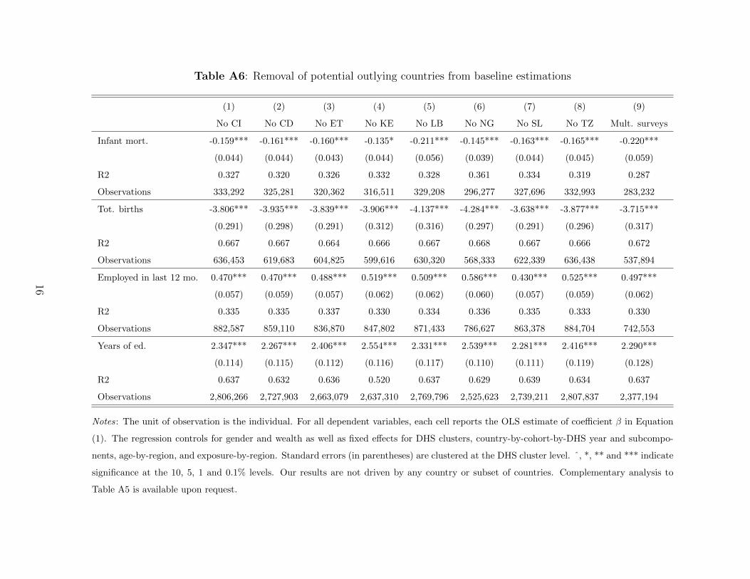
Table A6: Removal of potential outlying countries from baseline estimations

(1) (2) (3) (4) (5) (6) (7) (8) (9)

No CI No CD No ET No KE No LB No NG No SL No TZ Mult. surveys

Infant mort. -0.159*** -0.161*** -0.160*** -0.135* -0.211*** -0.145*** -0.163*** -0.165*** -0.220***

(0.044) (0.044) (0.043) (0.044) (0.056) (0.039) (0.044) (0.045) (0.059)

R2 0.327 0.320 0.326 0.332 0.328 0.361 0.334 0.319 0.287

Observations 333,292 325,281 320,362 316,511 329,208 296,277 327,696 332,993 283,232

Tot. births -3.806*** -3.935*** -3.839*** -3.906*** -4.137*** -4.284*** -3.638*** -3.877*** -3.715***

(0.291) (0.298) (0.291) (0.312) (0.316) (0.297) (0.291) (0.296) (0.317)

R2 0.667 0.667 0.664 0.666 0.667 0.668 0.667 0.666 0.672

Observations 636,453 619,683 604,825 599,616 630,320 568,333 622,339 636,438 537,894

Employed in last 12 mo. 0.470*** 0.470*** 0.488*** 0.519*** 0.509*** 0.586*** 0.430*** 0.525*** 0.497***

(0.057) (0.059) (0.057) (0.062) (0.062) (0.060) (0.057) (0.059) (0.062)

R2 0.335 0.335 0.337 0.330 0.334 0.336 0.335 0.333 0.330

Observations 882,587 859,110 836,870 847,802 871,433 786,627 863,378 884,704 742,553

Years of ed. 2.347*** 2.267*** 2.406*** 2.554*** 2.331*** 2.539*** 2.281*** 2.416*** 2.290***

(0.114) (0.115) (0.112) (0.116) (0.117) (0.110) (0.111) (0.119) (0.128)

R2 0.637 0.632 0.636 0.520 0.637 0.629 0.639 0.634 0.637

Observations 2,806,266 2,727,903 2,663,079 2,637,310 2,769,796 2,525,623 2,739,211 2,807,837 2,377,194

Notes: The unit of observation is the individual. For all dependent variables, each cell reports the OLS estimate of coefficient β in Equation

(1). The regression controls for gender and wealth as well as fixed effects for DHS clusters, country-by-cohort-by-DHS year and subcompo-

nents, age-by-region, and exposure-by-region. Standard errors (in parentheses) are clustered at the DHS cluster level. ˆ, *, ** and *** indicate

significance at the 10, 5, 1 and 0.1% levels. Our results are not driven by any country or subset of countries. Complementary analysis to

Table A5 is available upon request.

16

References

Acemoglu, Daron, and Simon Johnson. 2007. “Disease and Development: The Effect

of Life Expectancy on Economic Growth.” Journal of Political Economy, 115(6): 925–985.

Basu, Kaushik. 1999. “Child Labor: Cause, Consequence, and Cure, with Remarks on

International Labor Standards.” Journal of Economic Literature, 37(3): 1083–1119.

Basu, Kaushik, and Pham Hoang Van. 1998. “The Economics of Child Labor.” The

American Economic Review, 88(3): 412–427.

Becker, Gary S. 1975. “Investment in Human Capital: Effects on Earnings.” In Human

Capital: A Theoretical and Empirical Analysis, with Special Reference to Education, Sec-

ond Edition. NBER.

Becker, Gary Stanley, and Harold Gregg Lewis. 1973. “On the interaction between

the quantity and quality of children.” Journal of Political Economy, 81: S279–S288.

Beegle, Kathleen, Rajeev Dehejia, and Roberta Gatti. 2009. “Why Should We Care

about Child Labor? The Education, Labor Market, and Health Consequences of Child

Labor.” The Journal of Human Resources, 44(4): 871–889.

Ben-Porath, Yoram. 1967. “The production of human capital and the life cycle of earn-

ings.” The Journal of Political Economy, 352–365.

Bhatt, S., D. J. Weiss, E. Cameron, D. Bisanzio, B. Mappin, U. Dalrymple,

K. E. Battle, C. L. Moyes, A. Henry, P. A. Eckhoff, and others. 2015. “The effect

of malaria control on Plasmodium falciparum in Africa between 2000 and 2015.” Nature,

526(7572): 207–211.

Bleakley, Hoyt. 2010. “Malaria eradication in the Americas: A retrospective analysis of

childhood exposure.” American Economic Journal: Applied Economics, 1–45.

Bleakley, Hoyt, and Fabian Lange. 2009. “Chronic disease burden and the interaction

of education, fertility, and growth.” The review of economics and statistics, 91(1): 52–65.

17

Currie, Janet. 2009. “Healthy, Wealthy, and Wise: Socioeconomic Status, Poor Health in

Childhood, and Human Capital Development.” Journal of Economic Literature, 47(1): 87–

122.

Currie, Janet, and Brigitte C. Madrian. 1999. “Chapter 50 Health, health insurance

and the labor market.” In . Vol. 3, Part C, , ed. BT Handbook of Labor Economics,

3309–3416. Elsevier.

Edmonds, Eric V, and Maheshwor Shrestha. 2014. “You get what you pay for: School-

ing incentives and child labor.” Journal of Development Economics, 111: 196–211.

Gething, Peter W., Anand P. Patil, David L. Smith, Carlos A. Guerra, I. R.

Elyazar, Geoffrey L. Johnston, Andrew J. Tatem, and Simon I. Hay. 2011. “A

new world malaria map: Plasmodium falciparum endemicity in 2010.” Malaria Journal,

10(378): 1475–2875.

Hazan, Moshe, and Hosny Zoabi. 2006. “Does longevity cause growth? A theoretical

critique.” Journal of Economic Growth, 11(4): 363–376.

Hong, Sok Chul. 2013. “Malaria: An early indicator of later disease and work level.”

Journal of Health Economics, 32(3): 612–632.

Jayachandran, Seema, and Adriana Lleras-Muney. 2009. “Life Expectancy and Hu-

man Capital Investments: Evidence from Maternal Mortality Declines.” The Quarterly

Journal of Economics, 124(1): 349–397.

Pathania, Vikram. 2014. “The impact of malaria control on infant mortality in Kenya.”

Economic Development and Cultural Change, 62(3): 459–487.

Pigott, David M., Rifat Atun, Catherine L. Moyes, Simon I. Hay, and Peter W.

Gething. 2012. “Funding for malaria control 2006–2010: a comprehensive global assess-

ment.” Malaria Journal, 11: 246.

Psacharopoulos, George. 1997. “Child Labor versus Educational Attainment Some Evi-

dence from Latin America.” Journal of Population Economics, 10(4): 377–386.

18

Rosenzweig, Mark R., and Junsen Zhang. 2009. “Do population control policies induce

more human capital investment? twins, birth weight and china’s “one-child” policy.” The

Review of Economic Studies, 76(3): 1149–1174.

Snow, Robert W, Emelda A Okiro, Peter W Gething, Rifat Atun, and Simon I

Hay. 2010. “Equity and adequacy of international donor assistance for global malaria

control: an analysis of populations at risk and external funding commitments.” The Lancet,

376(9750): 1409–1416.

Soares, Rodrigo R. 2005. “Mortality reductions, educational attainment, and fertility

choice.” American Economic Review, 580–601.

19