Normal forms near a saddle-node andapplications to finite cyclicity of graphics

F. Dumortier, Y. Ilyashenko and C. Rousseau

CRM-2697

October 2000

Limburgs Universitair Centrum, Universitaire Campus, B-3590, Diepenbeek, BelgiqueDepartment of mathematics, Cornell University, Ithaca, New York 14853, U.S.A.

Departement de Mathematiques et de statistique and CRM, Universite de Montreal, C.P. 6128, Succursale Centre-Ville,Montreal, Qc, H3C 3J7, Canada.

The second author was supported by part by the grants RFBR 98-01-00455, NSF DMS 997-0372, CDRF RMI-2086. Thethird author was supported by NSERC and FCAR in Canada.

Abstract

In this note we refine the transformation to smooth normal form for an analytic family of vectorfields in the neighborhood of a saddle-node. This refinement is very powerful and allows to provethe finite cyclicity of families of graphics (“ensembles”) occuring inside analytic families of vectorfields. It is used in [RZ1] to prove the finite cyclicity of graphics through a nilpotent singular pointof elliptic type. Several examples are presented: lips, graphics with two subsequent lips, graphicswith a nilpotent point of elliptic type and a saddle-node. We also discuss the bifurcation diagram oflimit cycles for a graphic in the lips.

Resume

Dans cette note nous raffinons la transformation a la forme normale pour une famille analytique dechamps de vecteurs au voisinage d’un col-nœud. Ce raffinement est tres puissant et permet de montrerla cyclicite finie de familles de graphiques (“ensembles”) apparaissant dans des familles analytiquesde champs de vecteurs. Il est utilise dans [RZ1] pour montrer la cyclicite finie de graphiques passantpar un point singulier nilpotent de type elliptique. Plusieurs exemples sont presentes : les “levres”,des graphiques avec deux secteurs “levres” et un graphique avec un point nilpotent de type elliptiqueet un col-nœud. On discute aussi le diagramme de bifurcation des cycles limites pour un graphiqueapparaissant dans les “levres”.

1. Introduction

In the study of planar vector fields the question of finite cyclicity of graphics is an important one. Twocurrents of research meet there.

On one hand the powerful theorem of Ilyashenko-Yakovenko [IY] proves that elementary polycycles havefinite cyclicity inside generic families of smooth vector fields. The genericity conditions appearing in thetheorem are implicit. Special theorems by many authors give specific genericity conditions on particulargraphics (and not on families of vector fields) yielding finite cyclicity inside smooth families of vector fields.The graphics may be elementary or not. However it can be very difficult in practice to check the genericityconditions for a particular graphic.

On the other hand it is conjectured [R1] that graphics occuring among analytic families depending ona finite number of parameters have finite cyclicity inside the given family. A variant of this idea is thebasis of the program [DRR] to prove that there exists a uniform bound for the number of limit cycles ofa quadratic system. Particular theorems exist proving the finite cyclicity of special graphics (for instancehomoclinic loops) inside analytic families depending on a finite number of parameters.

The present note is a contribution to both directions in the particular context of analytic vector fields.We focus our attention to graphics which occur in “ensembles”. The idea is to consider the full “ensemble”(family of graphics), including the bordering graphic(s) which may or may not have higher codimension.We exploit additional data available or easily computable in the neighborhood of the bordering graphic(s)and “push” the information by analytic extension to all graphics of the “ensemble”.

As far as the second direction is concerned the method presented here is very powerful. In particular ithas allowed substantial progress in the proof of the finiteness part of Hilbert’s 16th problem for quadraticvector fields, namely the existence of a uniform bound for the number of limit cycles for quadratic systems.The problem has been reduced to the proof that 121 graphics have finite cyclicity inside quadratic systems[DRR]. In that spirit the results of Section 2 have allowed to prove in [DGR] the finite cyclicity of graphics(I2

14a) and (I215a) among quadratic systems (names from [DRR]). In this paper we apply our theorem of

finite cyclicity of a graphic through a nilpotent elliptic point and a saddle-node (Figure 1) to the graphic(I2

10a) inside quadratic systems (Figure 2).The results of section 2 are also used in [RZ1] to prove the finite cyclicity of an hp-graphic (i.e starting

from a hyperbolic sector and ending in a parabolic sector) through a nilpotent elliptic point. They willbe essential to prove the finite cyclicity of 12 more graphics: (F 1

6b), (I217b), (I1

5b), (I218b), (H3

10), (I17b), (I1

8b),(I2

26), (I110b), (I2

39), (I111a) and (I2

40), mostly treated in [RZ2]. In all cases the basic idea is that, whenconsidering ensembles, it may happen that, although a genericity condition on a regular transition mapcannot be calculated in general, it can be calculated on a particular graphic of the family. Then, usinganalyticity, it is possible to push the genericity condition to all graphics of the ensemble.

In [IY1] integrable Ck normal forms for unfoldings of saddle-nodes were found. These normal formsallow the explicit calculation of Dulac maps in the neighborhood of the singular point. In this paper weimprove this theorem for analytic vector fields: it is possible to choose the normalizing coordinates to beanalytic for the critical parameter value everywhere near the saddle-node except for the stable (unstable)one-dimensional invariant manifold passing through the saddle-node itself.

The genericity condition that implies finite cyclicity is formulated as the nonlinearity of some maps alongthe orbits, written in the normalizing charts. The main trick used in the paper is that the nonlinearity ofan analytic map may be established far away from the domain where it is used and then ”pushed forward”by analytic extension.

In this way we establish finite cyclicity of graphics that occur in ensembles. The main ensemble underconsideration is called “lips”; it is formed by two saddle nodes of opposite attractivity with a connectionbetween two hyperbolic sectors and a continuous family of connections between two parabolic sectors, seeFigure 3a. The name was given in [KS], where the ensemble is met under the number (3.13) of the “Kotovazoo” of graphics appearing in typical 3-parameter families of planar vector fields. Without increasing thedegeneracy of the vector field one can meet special graphics on the boundary of the ensemble. Denotethe orbit (part of the graphic) that connects two saddle-nodes through their hyperbolic (resp. parabolic)sectors as hh- (resp. pp-) connection. If an orbit emerges from one saddle-node through its parabolicsector and enters another one along the boundary between its hyperbolic and parabolic sector it is labeledas a bp-connection. Lips with a pp-connection through a saddle and lips with a bp-connection are shown

5

Figure 1. Graphic with pp-passage through a nilpotent elliptic pointand a saddle-node

Figure 2. Graphic (I110a) inside quadratic systems

in Figure 3b, c.We prove the finite cyclicity of any graphic of the ensemble “lips” in an analytic family under one of the

following conditions:

• the ensemble has a pp-connection through a saddle (Figure 3b) with either the hyperbolicity ratior not equal to 1 or with r = 1, but with no analytic first integral near the saddle;

• the ensemble has a bp-connection (no extra assumption on the corresponding boundary graphic isrequired.) As a corollary we obtain the finite cyclicity of any graphic in the ensembles “spadesuit”and “malignant frown”, names from [KS], see Figure 4.

Moreover, we prove the finite cyclicity of any graphic in the ensemble combined by two lips with two hh-6

Figure 3. Ensembles of graphics of “lips” type

Figure 4

connections, (see Figure 5) under a genericity condition. In analytic vector fields the genericity conditioncan as before be proved locally and pushed far away by analytic extension.

Figure 5. Graphics with two lips sectors

Finally in section 5 we discuss the bifurcation diagram for limit cycles appearing by perturbation of agraphic of the lips when the graphic has codimension n + 1, i.e. the transition map is nonlinear of ordern along the graphic. In that case the graphic has absolute cyclicity n and the bifurcation diagram of thelimit cycles contains a trivial 1-parameter family of elementary catastrophies of codimension n− 1.

In view of applying our results in specific situations we tackle the problem of calculating the regularpp-transition R. We show, in section 6, the existence of an integral expression of the derivative dR

dy (y, λ).The formula is an extension of the traditional formula of Poincare to express the derivative of a Poincaremapping along a regular piece of orbit. At the end of section 6 the formula is applied to a specific example.

2. Unfoldings of analytic germs of planar saddle-node vectorfields and analytic properties of their normalizations.

Unfoldings of germs of planar saddle-node vector fields with singular points of finite multiplicity may betransformed to a polynomial integrable normal form [IY]. The normalizing transformation may be taken

7

finitely smooth in a neighborhood of a singular point and critical parameter value in the phase-parameterspace; the smaller the neighborhood, the smoother will be the transformation. It is impossible, in general,to find an analytic normalizing transformation in some neighborhood, not even a C∞ one.

Yet some problems of bifurcation theory require analytic properties of the above normalizing transfor-mation. Below we prove the existence of a normalization for the above unfolding which is finitely smoothin the phase–parameter space but which is analytic in the phase space outside the (un)stable manifoldat the critical value of the parameter. This result may be applied to the proof of finite cyclicity of someplanar polycycles of analytic vector fields as it is shown in the subsequent sections.

2.1. Partially analytic normalization.

A saddle-node is a singular point of a planar vector field at which exactly one eigenvalue is zero. Ananalytic planar saddle-node germ v of multiplicity µ + 1 is formally orbitally equivalent by means of atransformation (x, y) 7→ (z, w) to a polynomial normal form

v0 = zµ+1(1 + azµ)−1 ∂

∂z− w

∂

∂w; (2.1)

the time orientation may be reversed. There exists a C∞ orbital equivalence between v and v0 [I1]. Anunfolding of a germ v, depending on the multi-parameter ε is finitely smoothly orbitally equivalent to thelocal family

vε = P (ε, z)∂

∂z+ zµ+1(1 + a(ε)zµ)−1 ∂

∂z− w

∂

∂w, (2.2)

with P (ε, z) =∑µ−1

i=0 bi(ε)zi where bi(0) = 0 [IY1].

To state our normalization theorem we need a preliminary normal form of an analytic saddle-node.

Proposition 2.1. Any complex saddle-node of multiplicity µ + 1 is orbitally analytically equivalent to agerm

v = v0 + zµ+1R(z, w)∂

∂w. (2.3)

This is the germ we will deal with. Main results of this section are the following.

Theorem 1. Consider a real analytic germ of a saddle-node vector field on (R2, 0) with one zero and onenegative eigenvalue and with even multiplicity. Then it is C∞ orbitally equivalent to its normal form (2.1).The equivalence may be taken analytic outside the stable manifold.

Theorem 2. Theorem 1 holds for germs with odd multiplicity.

Theorem 3. For any C∞ unfolding of a germ from Theorems 1,2 there exists a finitely smooth orbitalequivalence with the polynomial normal form (2.2). For the critical parameter value this equivalence isanalytic outside the stable manifold of the saddle-node germ.

Remark. If the germs of the vector fields in Theorems 1 and 2 (resp. the germ of the family in Theorem3) depend in an analytic way on extra parameters, not changing the nature of the germ (resp. the family),nor the “formal invariant” a(0) (i.e. a(ε) ≡ a(0)), then the equivalences may be taken analytic in both thevariables and the extra parameters in the regions described in the respective theorems.

Theorem 1 is proved below in 2.2 - 2.6. Theorem 2 is a free byproduct of the proof of Theorem 1.Theorem 3 is a simple corollary of Theorems 1 and 2, see 2.7, 2.8.

8

2.2. Sectorial normalization theorem.The sectorial normalization theorem (proved in [HKM] and presented in [MR], [I2]) claims that germs

v and v0 are analytically equivalent in some sector-like domains. These domains are described as follows.Let us divide a small disk |z| < r in 2µ equal sectors with vertex 0; the real axis contains some division

rays. Enumerate them counterclockwise beginning with the sector number 1 adjacent from above to thepositive real semiaxis. For any sector of this division consider a sector Sj with the same number andbisector, and with opening angle α ∈ (π

µ ,2πµ ). The sectors Sj , j = 1, . . . , 2µ are called good ones. They

form the covering of the punctured disk |z| < r. Let D = {|w| < r} be a disk in the w axis, andSj = Sj ×D.

Theorem 2.2 (see [HKM], [MR], [I2]). Any germ v, see (2.3) in a sector Sj (with r small) is analyticallyequivalent to v0. Moreover, the normalizing map Hj : Sj → C2 has the following properties:

1. Hj preserves z:Hj(z, w) = (z, hj(z, w)),

and brings v to v0;2. hj has asymptotic Taylor series in z with coefficients which are holomorphic functions in w:

h =∞∑0

ak(w)zk, a0(w) ≡ w;

h is the same for all hj;3. Maps Hj with these properties are unique.

The tuple H = (H1, . . . ,H2µ) is called the normalizing atlas of the germ v. Its transition functionsgenerate the Martinet–Ramis modulus of the analytic classification of complex saddle-nodes.

Let us call a germ (2.3) real if it is real on the real plane.

2.3 Normalizing atlas and Martinet–Ramis modulus.We do not need to give the complete construction of the above modulus. We only need part of this

construction; it is described below.The (multivalued) function

F (z, w) = wfa(z), fa(z) = e−1

µzµ za

is the first integral of the germ v0. Hence, the function

Fj = hjfa (2.4)

is the first integral of the germ v in Sj . In the intersection of their domains, one integral in this list is aholomorphic function of another. We will apply this to two pairs: Fµ, Fµ+1 and F1, F2µ, thus covering thetwo real semi-axes in the z-plane. Denote by S− and S+ the two sectors:{

S+ = S1 ∩ S2µ ∩ {Re z > 0}S− = Sµ ∩ Sµ+1 ∩ {Re z < 0}.

Case µ odd. Hence, fa → 0 on S+ as z → 0, fa →∞ on S− as z → 0.By the previous remark on the first integrals, there exists a holomorphic function ψ− such that in

S− ×Dhµ+1fa = ψ−(hµfa).

Let ψ−(u) = ψ0 + ψ1u+ ψ2(u)u2. Then

hµ+1(z, w) = ψ0f−1a (z) + ψ1hµ(z, w) + fa(z)ψ2(hµfa)h2

µ. (2.5)9

By statement 2 of Theorem 2.2, hµ+1 → w, hµ → w as z → 0. But in S−, fa → ∞ as z → 0. Hence, ψ0

may be arbitrary, ψ1 = 1 and ψ2 ≡ 0. Summarizing, we get

ψ−(w) = w + C (2.6)

hµ+1(z, w) = hµ(z, w) + Cf−1a (z). (2.7)

The constant C is one component of the Martinet–Ramis modulus.A parallel consideration gives the relation between h1 and h2µ, but the result is different because the

function fa on the sector S+ behaves in an opposite way than on S−. A second difference comes from thefact that fa(z) is multi-valued. Hence if we want to compare the value of fa(z) on S2µ, call it fa(z), withthe value of fa(z) on S1 we have, on S1 ∩ S2µ, fa(z) = νfa(z) with ν = exp(2πia) 6= 0. Hence we have:

h2µfa = ψ+(h1fa).

Let ψ+(w) = ψ0 + ψ1(w) + ψ2(w)w2. Then an analogue to formula (2.5) holds with hµ+1, hµ replaced byh2µ, h1. As before, h2µ → w, h1 → w as z → 0 in S+. But now fa → 0, f−1

a →∞ as z → 0 in S+. Hence,ψ0 = 0, ψ1 = ν(= exp(2πia)), ψ2 may be an arbitrary function. Summarizing, we get

h2µ = f−1

a ψ+(h1fa) = ν−1f−1a ψ+(h1fa),

ψ+(0) = 0, ψ+′(0) = ν,(2.8)

and ψ+ is an arbitrary holomorphic function with the above restriction. Roughly speaking, the functionψ+ is another component of the Martinet–Ramis modulus.

Case µ even. The origin is a topological saddle and we have the same behaviour in S± as the behaviourdescribed above on S+.

2.4. Martinet–Ramis modulus in the real case.

Let us call a germ v real if it is real on the real plane.

Proposition 2.3. If the germ v is real, then

hµ(z, w) = hµ+1(z, w), h1(z, w) = h2µ(z, w). (2.9)

Proof. By assumption, v is invariant under the involution (z, w) 7→ (z, w) in the source and the target. Bythe uniqueness of the normalizing atlas, see Theorem 2.2, H has the same property:

hµ−k(z, w) = hµ+k+1(z, w), k = 0, . . . , µ− 1.

This proves the proposition. �

Proposition 2.4. For the real germ v, the constant C in (2.6) is purely imaginary, and Imhµ(x, y) =iC2 f

−1a (x).

Proof. Let (x, y) ∈ R2. By (2.7) and (2.9)

i Imhµ(x, y) = −i Imhµ+1(x, y) = −C2f−1

a (x).

Hence, C is purely imaginary. �

10

Proposition 2.5. Fix an arbitrary positive x0 ∈ S+ and let g(w) = h1(x0, w). Let β = g−1(0). Then βand g′(β) are real.

Proof. Letg1(w) = h2µ(x0, w), c = fa(x0).

Then, by (2.8)cνg1 = ψ+(cg), ψ+(0) = 0, ψ+′(0) = ν. (2.10)

By (2.9),g(w) = g1(w). (2.11)

By (2.10) and (2.11), g(β) = 0 implies g1(β) = 0 = g1(β). As g1 is one-to-one, β = β, hence β is real.By (2.10)

cνg′1(β) = ψ+′(0)cg′(β),

hence, g′1(β) = g′(β). By (2.11), and reality of β,

g′(β) = g′1(β).

Hence, g′(β) is real. �

Remark. The same holds for hyperbolic sectors if µ is odd.

2.5. Automorphisms of the normalized germ.

Proposition 2.6 for parabolic sector. Consider an arbitrary complex number C− and let

H−(z, w) = (z, h−(z, w)), h−(z, w) = w + C−f−1a (z). (2.12)

Then H− is an automorphism of the germ v0 in S− = S− ×D;

(H−(z, w)− (z, w))|S− is flat on z = 0. (2.13)

Proof. The map H− preserves the z-coordinate and permutes the level curves of the first integral F =wfa(z) of the germ v0. Hence, it preserves the germ itself.

Statement (2.13) follows from the analogous property of f−1a : it tends to zero together with all deriva-

tives when z → 0 in S−. �

Proposition 2.7 for hyperbolic sector. Let ϕ be an arbitrary holomorphic function with ϕ(0) =0, ϕ′(0) = 1. Let

H+(z, w) = (z, h+(z, w)), h+(z, w) = f−1a (z)ϕ(wfa(z)). (2.14)

Then H+ is an automorphism of the germ v0 in S+ = S+ ×D;

(H+(z, w)− (z, w))|S+ is flat on z = 0. (2.15)

Proof. H+ preserves v0 for the same reason as H−.Statement (2.15) follows from the analogous property of fa in S+. Namely, let ϕ(w) = w + ϕ2(w)w2.

Thenh+(z, w) = w + fa(z)ϕ2(wfa(z))w2.

This implies (2.15). �

11

2.6. Smooth normalization of a saddle-node germ analytic outside the stable manifold foreven multiplicities.

Here we prove Theorem 1. A real saddle-node (2.3) with even multiplicity has three sectors: oneparabolic and two hyperbolic. The stable invariant manifold separates them. In the preliminary normalform (2.3) it is x = 0. We will call the union of two hyperbolic sectors in x > 0 the hyperbolic part (of theneighborhood of the saddle-node).

The normalizing map H will be constructed separately in the open parabolic sector (x < 0) and in thehyperbolic part. Both maps will be analytic in their domains and have flat difference with the identity onx = 0. Hence, after extension by the identity at x = 0, one becomes a C∞ continuation of the other.

In the parabolic sector let H = H− ◦Hµ, where Hµ is the same as in Theorem 2.2, H− is as in (2.12)with the constant C− well chosen. Namely, let Hµ = (z, hµ), C be the same as in (2.6). Then let C− = C

2 ,where C is the component of the Martinet–Ramis modulus, the same as in Proposition 2.4. Then H− isan automorphism of v0 in S− × D by Proposition 2.6. Hence, H conjugates v and v0 in the parabolicsector and is real there. Namely, by Proposition 2.4,

H(x, y) = (x,Rehµ(x, y))

in the parabolic sector.Let us now construct the map H in the hyperbolic part. It will be taken in the form H = H+◦H1, where

H1 comes from the Sectorial Normalization theorem, H+ is an automorphism provided by Proposition 2.7for a well chosen ϕ. LetH1(z, w) = (z, h1(z, w)), x0 > 0 be an arbitrary small number and g(y) = h1(x0, y).

Let k(y) = Re g(y) as in Proposition 2.5; k may be holomorphically extended to the complex domain.Let

ϕ = k ◦ g−1.

Then ϕ(0) = 0 and ϕ′(0) = 1. The map H+ given by (2.14) is an automorphism of v0 by Proposition 2.7.Hence, H = H+ ◦ H1 brings v to v0. Moreover, H is real on the segment σ : x = x0. As H conjugatestwo real vector fields v and v0, it is real in the saturation of σ by the phase curves of v, hence, in thehyperbolic part x > 0 of the neighborhood of zero.

Both maps H+ and H− differ from the identity by a map flat on x = 0. The maps Hµ and H1 have thesame asymptotic expansions on x = 0, see statement 2 of Theorem 2.2. Hence, the map H defined aboveseparately in the parabolic sector x < 0 and the hyperbolic part x > 0 continued by the identity at x = 0is C∞ smooth. It is real and brings v to v0. Theorem 1 is proved.

Proposition 2.8. When v has an analytic center manifold the constant C in (2.6) takes the value C = 0.

Proof. If the system has an analytic center manifold w = k(z), then modulo a change of variable w 7→w−k(z) in (2.3) R(z, w) factors as R(z, w) = wR1(z, w). This yields in Theorem 2.2 that h factors throughw, i.e. all aj(0) = 0. The curve y = 0 represents a level curve of the first integral (2.4). As obviously thefunction y = 0 is univalued as a function of x there can be no change of determination yielding that C = 0in (2.6). �

2.7. Saddle-nodes of odd multiplicity.Here we prove Theorem 2. A real saddle-node with odd multiplicity is topologically equivalent to a

saddle. Consider a germ (2.3). It has two hyperbolic parts x > 0 and x < 0 and a stable manifold x = 0.The desired conjugacy on (x > 0) is exactly the same as in the proof of Theorem 1, see 2.6. The conjugacyin x < 0 is now constructed in the same way as in x > 0. As before let the conjugacy be the identity onx = 0. The transformation thus constructed is C∞ for the same reason as in 2.6. Theorem 2 is proved.

2.8. Partially analytic normalization of unfoldings of saddle-nodes.Here we prove Theorem 3.Step 1. Let ε be the (multidimensional) parameter of the unfolding. Let us normalize the saddle-node

for ε = 0 according to Theorems 1,2, and extend the normalizing transformation cylindrically in ε. Wewill get a family of vector fields normalized on the plane ε = 0. The normalizing transformation on ε = 0has the required properties.

12

Step 2. Now we can transform the new family to the form

vε = w(x, ε)∂

∂x− T (x, ε)y

∂

∂y,

v0 has the normal form (2.1) (in particular, T (x, 0) ≡ 1), by a finitely smooth map, identical on ε = 0 [B].Division by T brings vε to

vε = w1(x, ε)∂

∂x− y

∂

∂y, w1(x, 0) = xµ+1(1− axµ)−1.

Step 3. The normalization procedure from [IY1], see also [IL],§9.2, allows us to normalize the familyw1(x, ε) ∂

∂x preserving w1(x, 0) by a finitely smooth map which is identical on ε = 0. The cylindric extensionin y of the latter map brings vε to the normal form (2.2).

The composition of maps constructed in Steps 1-3 provides the desired transformation.

3. Finite cyclicity of graphics occuring in the lips

To prove the finite cyclicity of the different graphics discussed in this section we bring the family of vectorfields to Ck normal form in the neighborhood of the singular points. We introduce sections transversal tothe graphics in the neighborhood of the singular points. We use the freedom of choice in the normalizingcoordinates to simplify the regular transitions defined on the sections. We introduce generic conditionson the regular transitions which are always defined (domain and image) in the normalizing coordinates.These generic conditions are always intrinsic (independent of the normalizing coordinates).

We repeat briefly the finite cyclicity proof for a particular graphic of the lips as it will be used later inSection 3 and in Sections 5 and 6.

3.1 Finite cyclicity of polycycles inside lips.

Theorem 3.1 [EM]. Consider a C∞ planar vector field v0 with an ensemble of graphics of the type “lips”:two saddle-nodes of opposite attractivity with one hh-connection, and a continuum of pp-connections.Suppose that the regular pp-transition, written in normalizing coordinates near the saddle-nodes has anonzero derivative of order n ≥ 2 at some point a (Figure 6). Then the graphic of the ensemble passingthrough a has finite cyclicity not greater than n.

Figure 6. Sections for the lips13

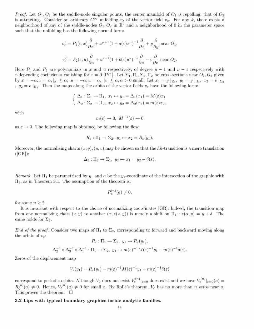
Proof. Let O1, O2 be the saddle-node singular points, the center manifold of O1 is repelling, that of O2

is attracting. Consider an arbitrary C∞ unfolding vε of the vector field v0. For any k, there exists aneighborhood of any of the saddle-nodes O1, O2 in R2 and a neighborhood of 0 in the parameter spacesuch that the unfolding has the following normal form:

v1ε = P1(ε, x)

∂

∂x+ xµ+1(1 + a(ε)xµ)−1 ∂

∂x+ y

∂

∂ynear O1,

v2ε = P2(ε, u)

∂

∂u+ uν+1(1 + b(ε)uν)−1 ∂

∂u− v

∂

∂vnear O2.

Here P1 and P2 are polynomials in x and u respectively, of degree µ − 1 and ν − 1 respectively withε-depending coefficients vanishing for ε = 0 [IY1]. Let Σ1,Π1,Σ2,Π2 be cross-sections near O1, O2 givenby x = −α;x = α, |y| ≤ α; u = −α;u = α, |v| ≤ α, α > 0 small. Let x1 = y |Σ1 , y1 = y |Π1 , x2 = v |Σ2

, y2 = v |Π2 . Then the maps along the orbits of the vector fields vε have the following form:{∆1 : Σ1 → Π1, x1 7→ y1 = ∆1(x1) = M(ε)x1

∆2 : Σ2 → Π2, x2 7→ y2 = ∆2(x2) = m(ε)x2,

withm(ε) → 0, M−1(ε) → 0

as ε→ 0. The following map is obtained by following the flow

Rε : Π1 → Σ2, y1 7→ x2 = Rε(y1),

Moreover, the normalizing charts (x, y), (u, v) may be chosen so that the hh-transition is a mere translation([GR]):

∆3 : Π2 → Σ1, y2 7→ x1 = y2 + δ(ε).

Remark. Let Π1 be parametrized by y1 and a be the y1-coordinate of the intersection of the graphic withΠ1, as in Theorem 3.1. The assumption of the theorem is:

R(n)ε (a) 6= 0,

for some n ≥ 2.It is invariant with respect to the choice of normalizing coordinates [GR]. Indeed, the transition map

from one normalizing chart (x, y) to another (x, z(x, y)) is merely a shift on Π1 : z(α, y) = y + δ. Thesame holds for Σ2.

End of the proof. Consider two maps of Π1 to Σ2, corresponding to forward and backward moving alongthe orbits of vε:

Rε : Π1 → Σ2, y1 7→ Rε(y1),

∆−12 ◦∆−1

3 ◦∆−11 : Π1 → Σ2, y1 7→ m(ε)−1M(ε)−1y1 −m(ε)−1δ(ε).

Zeros of the displacement map

Vε(y1) = Rε(y1)−m(ε)−1M(ε)−1y1 +m(ε)−1δ(ε)

correspond to periodic orbits. Although V0 does not exist V (n)ε |ε=0 does exist and we have V (n)

ε |ε=0(a) =R

(n)0 (a) 6= 0. Hence, V (n)

ε (a) 6= 0 for small ε. By Rolle’s theorem, Vε has no more than n zeros near a.This proves the theorem. �

3.2 Lips with typical boundary graphics inside analytic families.14

Theorem 3.2.(1) If the ensemble formed by lips has a pp-boundary graphic passing through a hyperbolic saddle inside

an analytic vector field then any graphic of the ensemble has absolute finite cyclicity as soon asthe saddle has hyperbolicity ratio r different from one or has no analytic first integral. (Thehyperbolicity ratio is the absolute value of the quotient of the negative eigenvalue to the positiveone).

(2) If the ensemble formed by lips has a bp-boundary graphic inside an analytic vector field then anygraphic of the ensemble has absolute finite cyclicity. In particular all graphics inside the malignantfrown or the spadesuit have finite cyclicity.

Proof. We need to prove in each case that the regular pp-transition written in normalizing coordinates hasa nonaffine ∞-jet at each point. This property is invariant under the choice of the normalizing coordinates.By Theorems 1 and 3 these coordinates may be chosen to be analytic on the cross-sections Π1 and Σ2.Hence, in these coordinates, R0 is analytic. To check that all its ∞-jets are nonaffine it is sufficient toprove that the map is nonaffine globally.

(1) To do that in case (1), let us consider the map R0 near the intersection of Π1 with the boundarygraphic Γ. Making a shift, we can consider the points Γ ∩ Π1 and Γ ∩ Σ2 to have zero y1 and x2

coordinates. Then, near 0,

R0(y1) =

{yr1(A+O(y1)), r 6= 1,

y1(A+∑i−1

j=1 cjyj1 +Byi

1 ln y1 +O(yi1)) for some i ≥ 1; r = 1,

with AB 6= 0. This map is not affine near zero. Hence, it is nonaffine everywhere, by analyticity.(2) In the case of a bp-boundary graphic the unstable manifold γ of one saddle-node, say O1, enters the

other saddle-node O2 as part of a center manifold. Without loss of generality, after a coordinateshift, if necessary, we may assume that R0(0) = 0. Let Σ2∩γ = a, D = [0, a]. Then all the positivesemi-orbits that begin near O1 in the domain being a square K : x1 ∈ [0, α], y1 ∈ [0, α], α is small,in the normalizing chart, intersect D. The map K → D along the orbits is analytic. Suppose thatΠ1 ⊃ {x1 = α, y1 ∈ [0, α]}, and the map R0 : Π1 → D is affine. As R0(0) = 0 it is linear; letR0(y1) = βy1. For any n > 2, let Πn = {x1 = α

n , y1 ∈ [0, α]}. The map Rn : Πn → D along theorbits of the ensemble is well defined and analytic. The map Πn → Π1 may be easily calculated,

because y1e1

µxµ1 x−a

1 is a first integral near O1. This map is a multiplication by

Cn = enµ−1µαµ na, Cn →∞

as n → ∞. Then the map Πn → D along the orbits is a multiplication by Cnβ. The lengthof the image is Cnαβ. It tends to infinity with n, but the image belongs to the segment D, acontradiction.

�

3.3 Two subsequent lips.

Theorem 3.3. A graphic of a C∞ vector field with four saddle-nodes of even multiplicity, alternatelyattracting and repelling, has finite cyclicity if the two regular pp-transitions satisfy the following genericconditions:

i) both are nonaffine at some finite order;ii) at some finite jet level one map is not right–left affine equivalent through orientation preserving

affine maps to the inverse of the other.An explicit bound for the cyclicity is given by the minimal order N of the jet of the two pp-transitions onwhich we can check the genericity condition.

If the two regular pp-transitions are analytic, then the theorem follows under the hypothesis that thetransitions are not affine and one map is not right–left affine equivalent through orientation preservingaffine maps to the inverse of the other. Indeed these conditions can be verified on a finite jet.

Proof. Denote the cross-sections in the parabolic sectors of the saddle-nodes as Σ1, Π1, Σ2, Π2, see Figure5.

15

Let fε : Σ1 → Π1, gε : Π2 → Σ2 be the pp-transitions corresponding to the value ε of the parameter(gε is the transition backwards). For those values of the parameter for which all the saddle-nodes vanish,the maps along the orbits of perturbed fields a : Π2 → Σ1, b : Σ2 → Π1 are affine in the normalizingcoordinates chosen above.

The displacement map has the form Vε : Π2 → R, Vε(x) = fε ◦ a− b ◦ gε.Let f = f0, g = g0. Theorem 3.3 follows now from the next Lemma. �

Main Lemma 3.4. Let functions f, g be CK diffeomorphisms on a segment, which are, at some finitejet level of order < K, nonaffine and not right–left affine equivalent through orientation preserving affinemaps. Then for any two points x0, y0 there exists N = N(f, g, x0, y0) < K, U, V small neighborhoods ofx0, y0 and small CN neighborhoods of f and g such that the function

ha,b = f ◦ a− b ◦ g

has no more than N zeros in U ∩ a−1V , where a, b are arbitrary orientation preserving affine maps.

Proof. Let x0 = y0 = 0, f (m)(0) = am, g(m)(0) = bm. Let a = αx+ α0, b = βx+ β0, ha,b = f ◦ a− b ◦ g.

Then h(m)a,b (0) = αmam − βbm.

Let α ≥ 1. Elsewhere we replace ha,b = 0 by an equivalent equation

b−1 ◦ f − g ◦ a−1 = 0

and use the symmetry of f and g in the assumptions of the theorem.Take k such that ak 6= 0. There exist at most a unique (α, β) such that h′a,b(0) = h

(k)a,b(0) = 0. Hence,

as f and g are not right-left affine equivalent, there exists n 6= k such that for all a and b

h′a,b(0) = h(k)a,b(0) = 0 =⇒ h

(n)a,b (0) 6= 0. (3.1)

Similar values k1 and n1 are obtained when we consider the case α ≤ 1 and we deal with the functionha,b = b−1 ◦ f − g ◦ a−1. We will prove that N(f, g, 0, 0) above may be chosen equal to max(n, k, n1, k1).

We will choose U and V so small that for any a and b and for any f , g CN -close to f, g one of thefollowing three inequalities holds on V ∩ a−1(U) : h′a,b 6= 0, h(k)

a,b 6= 0, h(n)a,b 6= 0.

That one of these inequalities holds depends on the relations between α, β and the derivatives of f andg at 0. Let ak > 0 (we can obtain that by replacing, if necessary, f and g by −f and −g respectively).

Case 1: bk < 0. In this case h(k)a,b > 0 on V ∩ a−1U for small U and V and f , g CN -close enough to f, g;

this assumption will not be repeated later on. Indeed,

h(k)a,b(x) = αkck − βdk > 0,

where ck is close to ak > 0, dk is close to bk < 0, α > 0, β > 0.Case 2: bk = 0. In this case either

h′a,b 6= 0 or h(k)a,b 6= 0 on V ∩ a−1(U). (3.2)

Let A1 = {(α, β) ∈ R2+ | αc1 − βd1 = 0} where c1, d1 range over small neigborhoods of a1, b1. For

(α, β) /∈ A1, the first inequality in (3.2) holds.For (α, β) ∈ A1, the set h(k)

a,b(x) = 0 is given by

Ak = {(α, β) ∈ R2+|αkck − βdk = 0},

where ck ranges in a small neighborhood of ak = f (k)(0), and |dk| < δ (dk ranges near bk = 0). Then for(α, β) /∈ Ak,

h(k)a,b 6= 0 on V ∩ a−1(U).

16

Moreover,{α ≥ 1} ∩A1 ∩Ak = ∅

for δ small enough. This proves (3.2). Hence, ha,b has no more than k zeros in V ∩ a−1(U).

Case 3: bk > 0. In addition to A1, Ak, consider a set

An = {(α, β) ∈ R2+|αncn − βdn = 0},

where cn, dn range near an, bn. The choice of n, see (3.1), implies that for c1, ck, cn, d1, dk, dn, closeenough to a1, ak, an, b1, bk, bn respectively

A1 ∩Ak ∩An = ∅.

Hence, either (3.2) holds, or h(n)a,b 6= 0. This proves the Main Lemma 3.4, hence, Theorem 3.3. �

The situation of Theorem 3.3 defines an ensemble of graphics with four semi-hyperbolic points indexedby an open subset of R2. We now give conditions so that any graphic of the ensemble occuring inside ananalytic vector field has finite cyclicity.

Corollary 3.5. A graphic of an analytic vector field with four saddle-nodes of even multiplicity alternatelyattracting and repelling has finite cyclicity if the two ensembles of lips are bounded simultaneous above(resp.below) by two pp-connections (one for each ensemble of lips), each through a hyperbolic saddle andif the two hyperbolic saddles belonging to the two boundary pp-transitions have hyperbolicity ratios r1 andr2 satisfying r1, r2 6= 1 and r1r2 6= 1 (Figure 7).

Figure 7

Proof. The two pp-transitions are nonaffine: this is the same argument as in Theorem 3.2. We need nowto show that one is not right-left affine equivalent to the inverse of the other. For that purpose we use thesame sections and notations as in Theorem 3.3 and Main Lemma 3.4.

The sections Σi and Πi can be taken analytic and so as to intersect the pp-boundaries passing through thehyperbolic saddles. Let I and J be the domains of definition of f0 and g0: these domains are open intervals.The intersection points X0 and Y0 of the upper pp-boundaries with the sections Σi are respectively thesupremum of I and J . The maps f0, g0 cannot be extended as diffeomorphisms above these points. Indeed,f0(X) = (X −X0)

r1(C + o(1)), r1 6= 1, C > 0. Hence, f ′0(X0) = 0 for r1 > 1 and f ′0(X0) = ∞ for r1 < 1.The same argument works for g0.

17

Let us suppose that we have a relation of the form

f0 ◦ a− b ◦ g0 = 0, (3.3)

where a and b are affine maps, the equality standing in the neighborhood of points y0 = a−1(x0). Therelation can also be written

f0 = b ◦ g0 ◦ a−1, g0 = b−1 ◦ f0 ◦ a. (3.4)

This defines analytic extensions of f0 on a(J) and of g0 on a−1(I). Let a(Y0) ∈ I. Then the first relationin (3.4) leads to a contradiction: f0 is diffeomorphic at a(Y0), and b ◦ g0 ◦ a−1 is not. If a−1(X0) ∈ J , thesecond relation in (3.4) provides a contradiction. If none of the case holds, then a(Y0) = X0. Then (3.3)yields:

(Y − Y0)r1(C1 + o(1)) = (X −X0)

1r2 (C2 + o(1))

which implies r1r2 = 1, a contradiction. �

Corollary 3.6. A graphic of a C∞ family of vector fields with an arbitrary number of saddle-nodes, allwith central transition, has finite cyclicity as long as there is no more than two pp connections and:

(1) the genericity assumption of Theorem 3.1 is satisfied in the case of one pp-connection;(2) the genericity assumption of Theorem 3.3 is satisfied in the case of two pp-connections.

Proof. When there are no pp-connection the saddle-nodes are all of the same attractivity and the graphicis known to have cyclicity one as the derivative of the Poincare map is far from 1. In the two other casesthe proof is exactly the same as the corresponding proof in Theorems 3.1 and 3.3. �

4. Graphic with a saddle-node and an elliptic nilpotent point

4.1 Finite cyclicity of such a graphic.

In the next paragraph we are concerned with the finite cyclicity of a graphic through a nilpotent pointof multiplicity 3 and of elliptic type inside a C∞ family of vector fields vε|{ε∈Λ}. In the neighborhood ofsuch a point the vector field v0 is C∞ equivalent to a vector field with 4-jet:

x = y

y = −x3 + bxy

where b > 2√

2.A weighted blow-up (x, y) = (rx, r2y) allows to study the topological type of the singularity (Figure 8).

On the blown-up circle we have two saddles and two nodes.

Figure 8. Nilpotent elliptic point and its blow-up18

We prefer to transform the singularity via the quasi-homogeneous change of coordinate (X,Y ) =(x

c ,1c (y − cx2)) to a system

X = Y + c2X2

Y = XY,

where 2c2 − cb + 1 = 0. Choosing c = b−√

b2−84 (this amounts to choose the bring the two nodes, called

P1 and P2, on the blown-up circle to the horizontal axis), letting c2 = a and renaming (X,Y ) by (x, y) westudy the singularity with a 4-jet of the form

x = y + ax2

y = xy(4.1)

with a ∈ (0, 12 ). The same weighted blow-up (x, y) = (rx, r2y) is used to draw it in Figure 9. The

advantage of this model is that the y-axis (corresponding to the direction of approach of the singular pointfor pp-transitions) is invariant.

Figure 9. Nilpotent point of (4.1) and its blow-up

The graphic we will study consists of a connection between the two nodes (for this reason we say that thegraphic has a pp-passage through the elliptic point) and an additional saddle-node Q3 on the connectionwhich we can of course suppose to be attracting (Figure 10).

The genericity condition concerns the passage (regular transition) from P2 to the saddle-node Q3: weconsider sections Σ and Π transversal to this transition map. These sections are taken parallel to onecoordinate axis in the normalizing coordinates near P2 and Q3.

Figure 10. Graphic with pp-passage through a nilpotent elliptic pointand a saddle-node

(P2 is considered in the chart x = 1. Hence the coordinates near P2 are r and y. As r = 0 is invariant anormalizing change of coordinates can be taken as a function of the form y = y+O(r)+o(y), which, as P2

is a node, can be taken analytic if v0 is analytic.) The regular transition is a map R : Σ → Π. Assumingthat the connection occurs for y = 0 the genericity condition allowing to prove the finite cyclicity is thatthere exists n ≥ 2 such that R(n)(0) 6= 0.

19

Remark. The condition is intrinsic. We need to show that the condition is invariant under changes ofcoordinates preserving the normal form near P2 and near Q3. Near Q3 the result follows from [GR]. NearP2 we use that P2 is a node with normal form (for ε = 0)

r = r

˙y = σy +Arn

where A = 0 as soon as σ /∈ N.Because of the special form of the system we only allow normalizing changes of coordinates keeping

r fixed. If σ /∈ N then there is no nonlinear change of normalizing coordinates. Indeed a sufficientlysmooth change of coordinate must preserve the analytic invariant manifold. Hence it has the form y 7→y1 = y(C + O(|(r, y)|)) and must send the first integral H(r, y) = r−σ y to φ(H). From σ /∈ N necessarilyφ(H) = CH, i.e. y1 = Cy. If σ ∈ N and A = 0 we can allow the change of coordinate to have the formy 7→ y1 = Cy + o(|(r, y)|). When A = 0, with the same H as before, we get φ(H) = CH + D. On asection r = r0 the first integral H (resp. φ(H)) is an affine map of the normalizing coordinate y (resp.y1). As φ is affine the result follows. We are left with the case σ ∈ N and A 6= 0 in which case the integralhas the form H(r, y) = y−Arσ ln r

rσ . The only allowed change of coordinate preserving the normal form isy 7→ y1 = y + o(|(r, y)|) and send H to φ(H) = H +D (which implies that y1 = y + Brσ). We concludeas before since H and φ(H) are still affine maps of y and y1 on r = r0.

If n is minimal with this property then we say that the map R is nonaffine of order n at y = 0.

Theorem 4.1. A graphic with central transition through a saddle-node and with pp-passage through anilpotent elliptic point of multiplicity 3 has finite cyclicity ≤ n as soon as the transition map from theelliptic point to the parabolic sector of the saddle-node (in normalizing coordinates, see the previous remark)is nonaffine of some finite order n (Figure 10).

Proof. We use the method of the blow-up of the family [DRS] and the notations introduced in [RZ1] andwe suppose that the saddle-node is attracting. In the neighborhood of the nilpotent elliptic point we canuse the following normal form for the family ([RZ1]):

x = y + a(ε)x2 + µ2

y = µ1 + µ3y + x4h1(x, ε) + y(x+ η2x2 + x3h2(x, ε)) + y2Q(x, y, ε),

(4.2)

where a(0) ∈ (0, 12 ) and η2 ∈ R. The parameters are ε = (µ1, µ2, µ3, µ), h1(x, ε) = η2a + O(ε) + O(x).

Moreover the functions h1(x, ε), h2(x, ε) and Q(x, y, ε) are C∞ and Q(x, y, ε) is of arbitrary high order in(x, y, ε).

We must discuss the number of limit cycles in a Hausdorff neighborhood of the graphic for values ofthe parameters in a small neighborhood of the origin. Only the parameters µi, i = 1, 2, 3, will be essentialto the results.

We make the change of parameters (µ1, µ2, µ3) = (ν3µ1, ν2µ2, νµ3) and consider a neighborhood of the

origin in the space (µ1, µ2, µ3) given by (µ1, µ2, µ3) ∈ S2 and ν ∈ (0, ν0).We will prove that for all µ∗ = (µ1, µ2, µ3) ∈ S2 and for any µ∗ there exist neighborhoods of µ∗ and µ∗,

there exist ν0 > 0 and δ > 0 such that for µ and µ respectively in the neighborhoods of µ∗ and µ∗ andfor ν < ν0 the family vε has at most n limit cycles at a Hausdorff distance distance less than δ from ourgraphic. We conclude using compacity of S2.

We identify (4.2) to a µ family of 3-dimensional systems by adding the additional equation ν = 0. Wetake two sections Σ1,2 = {x = ∓x0} in the neighborhood of the nilpotent point and consider the twotransitions S : Σ2 → Σ1 and T : Σ1 → Σ2 (Figure 11).

The first transition S is quite standard, except for the fact that Σi are two dimensionsal sectionsparametrized by (ν, yi), i = 1, 2, where yi are normalized coordinates coinciding for ν = 0 with yi definedbefore near Pi (details below). The transition T is not standard as it describes the passage near a non

20

Figure 11. The sections Σ1 and Σ2 close to the blown-up sphere

elementary singular point. To study it we use the blow-up of the family introduced by Roussarie andapplied in [DRS] and [RZ1].

In the neighborhood of the origin we apply the weighted blow-up (x, y, ν) = (rx, r2y, rρ) where r ≥ 0and (x, y, ρ) ∈ S2, to the system (4.2) to which we have added the equation ν = 0. This blows up theorigin to a sphere (corresponding to r = 0) which is invariant under the flow. Moreover from ν = 0 we getthat the function rρ is invariant under the flow. The singular locus rρ = 0 is formed by the plane ρ = 0parametrized by (x, y) ∈ S1 and r (r = 0 corresponds to the weighted blow-up of the singularity of (4.2) asε = 0) together with the sphere r = 0, (x, y, ρ) ∈ S2. Because of the geometry the flow has to be studiedin charts.

The idea of the method is to study the flow on the singular locus for the different values of the µi. Tostudy the flow on the sphere r = 0 we work in charts. The chart ρ = 1 is called the family rescaling whilethe charts x = ∓1 (or y = ±1) allow to study the neighborhood of the circle r = ρ = 0 (which correspondsto the usual weighted blow-up of the singularity for ε = 0).

The chart ρ = 1 provides phase portraits on the sphere for the different values of µi. In the chartsx = ∓1 we study the neighborhood of the four singular points Pi, i = 1, . . . 4. These are the points atinfinity in the chart ρ = 1 (infinity being studied in weighted coordinates). Glueing that with the globaltrajectories outside the neighborhood of the singular point yields limit periodic sets in 3-dimensional space.

In the chart ρ = 1 the system has the form

x = y + ax2 + µ2

y = xy + µ1 + µ3y +O(r).(4.3)

The method consists in identifying all limit periodic sets which we will encounter in the singular set rρ = 0and in studying the finite cyclicity of each of them. In our case we find the three limit periodic setsappearing in Figure 12 (see also Figure 13 for a 3-dimensional picture). They have to be studied in athree dimensional space, the disk in the middle being the upper half-sphere r = 0, ρ ≥ 0. The use of theinvariant foliation ν = rρ = const allows in practice to reduce the study to 2 dimensions.

The points P1 and P2 considered previously now become singular points of a 3-dimensional vector field.Looking at them in the respective charts x = ±1, natural coordinates in their neighborhood are givenby (r, ρ, yi). The eigenvalues are given by ∓a(ε),±a(ε),∓(1 − 2a(ε)). Hence the normal form dependswhether a(0) is rational or irrational. We will treat in detail the simpler case a(0) /∈ Q which contains allthe essential ideas. One ingredient is the orbital normal form near P1 and P2. When a(0) /∈ Q the onlyresonance is between the first two eigenvalues. Because of the invariant foliation the Ck orbital normalform is given by

r = ∓rρ = ±ρ˙yi = ∓σyi + yif

±ε (rρ)

(4.4)

where σ = 1−2a(ε)a(ε) and f±ε (rρ) = f±ε (ν) =

∑ki=1 a

±i (ε)νi.

Let us come back to the sections Σ1,2 = {x = ∓x0} defined previously. In the respective charts x = ±1they correspond to sections with respective equations r = x0, where r0 = ρ0. Coordinates on the sections

21

Figure 12. The limit periodic sets Epp1, Epp2 and Epp3. The smalldisk represents the upper half-sphere seen from above

Figure 13. The limit periodic set Epp2 and its sections in 3-dimen-sional space

22

are ν (related to ρ through ν = r0ρ) and the variable yi defined in (4.4). Then yi = yi+o(yi)+O(r)+O(ρ) =1r20(yi + o(yi)) depends in a Ck way of yi and the parameters.Using the blow-up of the family we can now calculate the transition map T : Σ1 → Σ2. Indeed

we decompose it into a composition of three transition maps: two transition maps (Dulac maps) in theneighborhood of P1 and P2 and a regular transition map T along the blown-up sphere: T = D−1

2 ◦T ◦D1,where Di : Σi → Πi.

At this point it is important to consider all phase portraits of (4.3). As soon as µ1 6= 0 there is nopassage from P1 to P2 on the sphere r = 0. Hence the only limit periodic sets listed above correspondto µ1 = 0, i.e. to the existence of an invariant line on which we have either no singular point (µ2 > 0)or a saddle-node (µ2 = 0, µ3 = ±1). The Dulac map corresponding to the passage near P1 (resp. nearP2 with reverse time) will be the transition map for system (4.4) with i = 1 (resp. i = 2) from thesection Σi = {r = r0} to a section Πi = {ρ = ρ0}, parametrized by (ν, yi) = (ρ0r, yi). The Dulac mapsDi : Σi → Πi are calculated from (4.4) as

Di(ν, yi) =(ν,

(ν

ν0

)σ

yi

(1 +

(e−f±ε (ν) ln ν

ν0 − 1)))

=(ν,

(ν

ν0

)σ

yi (1 +Ni(ν, ln ν, ε)))

where Ni(ν, ln ν, ε) = −a±1 (ε)ν ln νν0

+O(ν2(ln ν)2) and ν0 = r0ρ0.The third component in the transition T is the transition map T : Π1 → Π2. The map is regular

if µ2 > 0, in which case, because of the invariant foliation, it has the form (ν, z) 7→ (ν, T (ν, z)) whereT ](ν, z) = A(ν)z+O(z2) with A(0) 6= 0. When µ2 = 0 it is the composition of two regular transition mapsand a linear map corresponding to the passage near a saddle-node through central transition. The globalform of T is the same as in the regular case but the coefficient A(ν) can be either very small or very largewhen µ2 varies.

We also have a Dulac map near the saddle-node Q3. Near Q3 the Ck normal form is taken as theproduct of the usual normal form (depending on ν) with the equation ν = 0. Hence the Dulac map hasthe form D3(ν, u) = (ν,m3(ε)u), where m3(ε) → 0 as ε→ 0.

Finite cyclicity of the limit periodic set Epp1. We consider the return map defined on section Σ1

in coordinates (ν, y1). The first coordinate is the map (ν, y1) 7→ ν while the second has a first derivativein y1 smaller than 1. This suffices to prove that Epp1 has cyclicity at most one.

Finite cyclicity of the limit periodic set Epp3. Here there is an additional attracting saddle-nodeQ4 on the line y = 0 on the blown-up sphere. The Dulac map near Q4 is similar to that of P3 with acoefficient m4(ε) such that m4(ε) → 0 as ε→ 0. As for Epp1 the cyclicity is at most 1.

Finite cyclicity of the limit periodic set Epp2. In this case we introduce sections Σi and Πi,i = 3, 4 near the two saddle-nodes so that the second component of the central transitions are of the formy3 7→ m3(ε)y3 and y4 7→M4(ε)y4 where

limε→0

m3(ε) = 0, limε→0

M4(ε) = +∞.

We can choose the normalizing coordinates near Q3 and Q4 so that the two transition maps from Π1 toΣ4 and from Π3 to Σ1 are mere translations. We are left with two Ck-transitions Rε : Σ2 → Σ3 andUε : Π2 → Π4. We consider the displacement map from Σ2 to Σ1. We only need to consider the secondcomponent which can be written as (we denote y2 simply by y):

Vε(y) = m3(ε)Rε(y) + δ1 −

((ν

ν0

)−σ

(M4(ε))−1Uε

((ν

ν0

)σ

y(1 +N2(ν)))

+ δ2

)(1 +N1(ν))−1.

The first derivative is given by

V ′ε (y) = m3(ε)R′ε(y)−M4(ε)−1U ′ε

((ν

ν0

)σ

y(1 +N2(ν)))

(1 +N1(ν))−1(1 +N2(ν)).

23

We consider the equivalent function

Wε(y) =R′ε(y)

U ′ε

((νν0

)σ

y(1 +N2(ν))) − (m3(ε)M4(ε))−1(1 +N1(ν))−1(1 +N2(ν)).

Then W (n−1)ε (y) 6= 0 for sufficiently small (y, ε).

The case a(0) ∈ Q is longer to write. However the Dulac maps near P1 and P2 have been studied indetail in [RZ1] (in particular the fact that they behave well under derivation). The theorems of [RZ1]ensure that all steps of the proof just done can be reproduced nearly verbatim in the new context. �

4.2 Application to quadratic vector fields.

Corollary 4.2. The graphic (I210a) (Figure 2) of quadratic systems has finite cyclicity.

Proof. Originally in [DRR] this graphic was noticed to occur in the family

x = λx− µy + a20x2 + a11xy + a02y

2

y = µx+ λy + b20x2 + b11xy + b02y

2

with (λ, µ) ∈ S1 and (a20, . . . , b02) ∈ S5. Using a rotation we can suppose that the hyperbolic singularpoint at infinity is located along the x-axis, yielding b20 = 0. By a linear transformation we can assumethat the nilpotent singular point is located along the y-axis, yielding a02 = 0. The point is nilpotent ifand only a11 = b02 = 0. Using that the origin is a focus, that the nilpotent point is of elliptic type withthe position of the separatrices as in Figure 2 and additional scaling we can finally see that the graphicoccurs in a quadratic system of the form:

x = δx− y +Ax2

y = x+ γy + xy

where A ∈ (12 , 1).

The additional condition (δ − γA)2 − 4A = 0 guarantees the existence of a point of multiplicity atleast two, so is satisfied when a graphic (I2

10a) occurs but this is not needed in the proof. It is easilychecked that the family of graphics through the saddle node ends in a graphic with a hyperbolic saddlewith hyperbolicity ratio less than 1. We must show that the map R0 of Theorem 3.3 is nonaffine on anygraphic of the family. As in Theorem 3.2 this will be proved by an analytic extension principle using thefact that the hyperbolicity ratio is different from 1. Indeed R0 is nonaffine near the limiting graphic whichpasses through the hyperbolic saddle. We can choose sections in the normalizing coordinates near thesaddle-nodes which are analytic. Moreover the point P2 of the blown-up sphere (Figures 9 and 10) witheigenvalues (1,−1, σ) is a node when restricted to the invariant plane ρ = 0. Hence the normalizing changeof coordinates near P2 can be taken as the composition of an analytic map: y 7→ y, bringing the node tonormal form in the plane ρ = 0 together with an additional change of coordinates depending on ρ andequal to the identity on the plane ρ = 0. The map R0 is defined between analytic sections parametrizedby analytic coordinates. We conclude that the transition map is nonaffine near the limiting graphic, hencenonaffine everywhere. �

5. Elementary catastrophies of limit cycles occuring in perturbations of the lips

5.1 Bifurcation diagram near a single graphic.In this section we will concentrate on the simplest situation in which the “lips” occur, namely the

configuration represented in Figure 3a, and already considered, with respect to the finite cyclicity problem,in Theorem 3.1. We will continue using some notions introduced in that theorem. Aiming at describinginteresting and stable patterns of limit cycles we will impose a number of genericity conditions, to bespecified in the text. All our local results – localized near one of the limit periodic sets in the ensemble

24

– do however also apply to the more complicated situations represented in the Figures 3 and 4. We willdeal with local C∞ ε-families of vector fields with ε ∈ Rp.

We locate the semi-hyperbolic point with repelling (resp. attractive) parabolic sector at p1 (resp. p2);we should in fact write p1(ε) and p2(ε) but will not do it for sake of simplicity in notation. For k > 0sufficiently large we use the respective Ck normal forms x1 = µ1(ε) +

r−1∑j=1

bj(ε)xj1 + xr+1

1 (1 + a1(ε)xr1)−1

y1 = y1

(5.1)

and x2 = −µ2(ε)−s−1∑j=1

bj(ε)xj2 − xs+1

2 (1 + a1(ε)xs2)−1

y2 = −y2(5.2)

with r, s ≥ 1 and odd. We suppose the chosen graphic to be represented by y1 = 0. In these localcoordinates we can now define the “rotational” parameter δ in the regular hh-transition. Let us recall fromthe proof of Theorem 3.1 that we can reduce the regular hh-transition to an affine map with constant termδ(ε).

Like in the proof of Theorem 3.1 we can also consider the regular pp-transition R(y1, ε) with respect tothe normal form (5.1) and (5.2). Let us introduce

ai(ε) =1i!∂iR

∂yi1

(0, ε)

for 2 ≤ i ≤ n, with k � n ≥ 2. As generic conditions we require that

an(0) 6= 0 (5.3)

and that the mapping

ε 7→ (δ, µ1, µ2, b1, . . . , br−1, b1, . . . , bs−1, a2, . . . , an−1)(ε) (5.4)

is a submersion at ε = 0.

Theorem 5.1. Let Γ be a graphic with two semi-hyperbolic points of even multiplicity (Figure 3a), occuringin a C∞ ε-family of planar vector fields. Suppose that the regular pp-transition (defined on sections parallelto the y-axes in the Ck normalizing coordinates (5.1) and (5.2)) is of order n at y1 = 0, ε = 0 like expressedin (5.3), and that ε is a generic parameter as defined in (5.4). Then, keeping µ1 > 0 and µ2 > 0, in anyHausdorff neighborhood W of Γ and in any neighborhood V of ε = 0, the bifurcation diagram of the limitcycles contains a trivial 1-parameter family of elementary catastrophies of codimension n− 1.

Remarks.(1) In this theorem we have not described the full bifurcation diagram, and this was on purpose. By

Theorem 3.1 we already know the cyclicity to be at most n. In Theorem 5.1 we do not only showthe cyclicity to be exactly n, but we also show that all possible stable bifurcations involving atmost n limit cycles will occur. We do not intend to study the matching and the interference ofthese bifurcations of the limit cycles with the bifurcations of the singularities in the unfolding ofthe semi-hyperbolic points p1 and p2.

Moreover, besides the bifurcations of limit cycles that are “interior” to the chosen y1-neighbor-hood of 0, there are also the bifurcations corresponding to a limit cycle escaping from the chosenneighborhood of the graphic, a problem which we will consider in paragraph 5.2.

(2) The functions b1(ε), . . . , br−1(ε), b1(ε), . . . , bs−1(ε) are not present in condition (5.4) in case thesemi-hyperbolic points p1 and p2 both are of codimension 1, i.e. r = s = 1.

(3) A complete description of the bifurcations of the polycycle ”lips” in generic 3-parameter familieswas obtained in [KS].

25

Proof of theorem 5.1. As a consequence of the genericity conditions (5.4) we can, for ε ∼ 0, change theparameter ε ∈ Rp to a new parameter

ε = (ε′, ν)

withε′ = (δ, µ1, µ2, b1, . . . , br−1, b1, . . . , bs−1, a2, . . . , an−1)

and ν ∈ Rp−q for q = r + s+ n− 1. Let us from now on take

b1 = . . . = br−1 = b1 = . . . = bs−1 = 0, ν = 0, (5.5)

and denote the remaining parameters by

λ = (δ, µ1, µ2, a2, . . . , an−1).

Let us write y instead of y1 (the y-coordinate is chosen in a way that y = 0 represents the graphic underconsideration for λ = 0).

Like in the proof of Theorem 3.1 we can consider the regular pp-transition R(y, ε) and the relateddisplacement function V (y, ε). We can suppose that R is of class Ck, with k finite but as large as we want.Let us restrict to the condition (5.5) and denote R(y, ε) and V (y, ε) by respectively R(y, λ) and V (y, λ).

Under all the conditions that we suppose, we can write

V (y, λ) = δm−1(λ) + (α(λ)−m−1(λ)M−1(λ))y + a2y2 + . . .+ an−1y

n−1 + an(λ)yn + Ψ(y, λ) (5.6)

for some α(λ) > 0 and with Ψ of class Ck, Ψ = O(yn+1), an(0) 6= 0 and k � n. Let us recall that

m(λ) = exp

− X∫−X

dx1

µ1 + x1h(x1, λ)

and

M(λ) = exp

X∫−X

dx2

µ2 + x2h(x2, λ)

,

for some well chosen X > 0, X > 0 and where h(x1, λ) = xr1(1 + a1(λ)xr

1)−1, resp. h(x2, λ) = xs

2(1 +a1(λ)xs

2)−1.

As such

∂m

∂µ1(λ) =

X∫−X

(1 +O(x1))dx1

(µ1 + x1h(x1, λ))2

·m(λ), (5.7)

which is strictly positive for µ1 > 0 and X sufficiently small. Similarly we can prove that M(λ) →∞ forµ2 → 0, and that ∂M

∂µ2(λ) < 0 for µ2 > 0 and X sufficiently small.

Let us now work along a curve defined by δ = 0, a2 = . . . = an−1 = 0 and α(λ) = m−1(λ)M−1(λ). Weconsider this curve for µ2 > 0, where, because of (5.7) and a related property on ∂M

∂µ2, we can suppose that

it is regular and that it tends to the origin in parameter space for µ2 → 0.We will now study the bifurcation of limit cycles near y = 0 along this curve in parameter space. For

that purpose we change expression (5.6) into

V (y, λ, η) = η1 + η2y + a2y2 + . . .+ an−1y

n−1 + an(λ)yn + Ψ(y, λ), (5.8)

meaning that besides the parameters λ we introduce independent parameters η = (η1, η2) that we will alsokeep close to zero. Expression V is Ck in (y, λ, η) and as such we can apply to it the preparation theoremin finite smoothness ([Ba], [L]):

V (y, λ, η) = F (y, λ, η)[yn +Bn−1(λ, η)yn−1 + . . .+B0(λ, η)] (5.9)26

for some Ck′ functions Bi, 0 ≤ i ≤ n − 1, vanishing at the origin and F with F (0, 0, 0) 6= 0. In fact ifwe want here some k′ sufficiently larger than n we might need to adapt the previously chosen k. Let uscontinue denoting k′ by k. Along the chosen curve the application

(δ, µ1) 7→ (η1, η2)

is a local diffeomorphism near (0, 0), for each fixed µ2 > 0 sufficiently small, and as such the same holdsconcerning

(δ, µ1, a2, . . . , an−1) 7→ (B0(λ, η), . . . , Bn−1(λ, η))

near (0, . . . , 0).For each fixed value µ2 > 0, sufficiently small, we will hence encounter a stable elementary catastrophy

of codimension n− 1 on the zeros of V (y, λ). �

5.2 Bifurcation diagram near an ensemble of graphics.

We continue studying the situation considered in the preceeding paragraph 5.1, but instead of merelylooking at y ∼ 0 we will keep y ∈ [Y1, Y2] for some choice Y1 < 0 < Y2. In this paragraph we aim at fullydescribing the bifurcation diagram of the limit cycles, as long as these do not interfere with the appearanceof singularities. We completely describe it in the particular case r = s = 1: it is Ck diffeomorphic tothe trivial product of a line segment with the bifurcation set of the zeros of the Complete Tchebychevsystem (1, y, . . . yn) on [0, 1]. The same proof provides the description of the bifurcation diagram in thegeneral case where one of r, s is greater than 1 as long as we suppose that the parameter ε ∈ Rp is suchthat b1(ε), . . . , br−1(ε), b1(ε), . . . , bs−1(ε) in (5.1) and (5.2) remain zero. Besides this we want to work asgenerically as possible. As such we keep condition (5.3), but change (5.4) into the requirement that

ε 7→ (δ, µ1, µ2, a2, . . . , an−1)(ε) (5.10)

is not only a submersion, but in fact a local diffeomorphism at ε = 0; we hence restrict to p = n+ 1. Wecan now state the following result:

Theorem 5.2. Let Γ be a graphic like in Theorem 5.1 occuring in an ε-family with ε ∈ Rn+1. Supposethat the regular pp-transition is of order n at y = 0, for ε = 0, as expressed by (5.3), and let k ∈ N. Letε be a generic parameter as defined by (5.10), and let all bi(ε) and bj(ε) in (5.1) and (5.2) be identicallyzero. If |Y1|, |Y2| are sufficiently small then the bifurcation set of the limit cycles given by y ∈ [Y1, Y2],µ1, µ2 > 0 and ε small is Ck diffeomorphic to the trivial product of a line segment with the bifurcation setof the zeros of the Complete Tchebychev System (1, y, . . . , yn) on [0, 1].

Proof. We follow the reasoning developed in the proof of Theorem 5.1 and adapt it slightly. Lookingat expression (5.9) we can observe that for (ε, η) ∼ 0 we could introduce (µ1, µ2, δ, B1, . . . , Bn−1, η1, η2)as independent parameters instead of (ε, η). Let us say that it holds for |ηi| ≤ E with i = 1, 2. Thebifurcations expressed by (5.9) are then independent of (µ1, µ2, δ). We recall that in fact η1 = δm−1(λ)and η2 = α(λ) − m−1(λ)M−1(λ). For fixed µ2 the map δ 7→ η1 has everywhere a nonzero derivative,while the same is true for µ1 7→ η2, if we fix also (δ, λ) and stay inside the region where (5.9) holds.Indeed, by (5.7) and the boundedness of ∂α

∂µ1(ε) and η2 the result easily follows. Outside this region,

either |η1| = |δm−1(λ)| ≥ E or |η2| = |α(λ)−m−1(λ)M−1(λ)| ≥ E. Considering expression (5.8) directlyit is clear that, for sufficiently small y, V (y, ε) will have no zeros for |η1| ≥ |η2|, while there will be atmost one zero for |η2| ≥ |η1|. In that region the limit cycle has to stay hyperbolic if it exists and since∂η1∂δ = m−1(λ) > 0 we see that disappearance of such a limit cycle occurs in the most generic way possible.These observations permit to finish the proof. �

27

6. Integral expression of the derivative of the regular pp-transition

6.1 General formula.As we have seen in section 3, in the presence of “lips” the regular pp-transition plays an important role

in the study of the cyclicity. We have seen in section 5 that it also plays an essential role in studying thebifurcations of the limit cycles. However it might be quite involved, if not to say technically impossibleto control directly – based on the proposed construction – the necessary conditions. Therefore in thisparagraph we are going to relate the regular pp-transition R, or more precisely its derivative R′, to someintegral, whose essential characteristics are often easier to deal with. Our reduction is based on Poincare’sformula (see e.g. [ALGM] or [Rc]) for the derivative of a transition map (Poincare map) near a regularorbit.

Let us consider a C∞-family of vector fields Xλ, with λ ∈ Rq, having for each λ a pp-connection betweensingularities p1(λ) and p2(λ). Like in section 2 and 3 we suppose that – by Ck orbital equivalence (withk > 0 sufficiently large) – we can write Xλ near p1(λ) and p2(λ) as the respective normal forms:{

x1 = xr+11 (1 + a1(λ)xr

1)−1

y1 = y1(6.1)

and {x2 = −xs+1

2 (1 + a1(λ)xs2)−1

y2 = −y2(6.2)

with r, s ≥ 1 and odd.

Theorem 6.1. Let Xλ be a C∞ λ-family of planar vector fields having semi-hyperbolic points p1(λ)and p2(λ) of even multiplicity with respective Ck normal forms (6.1) and (6.2); k > 0 is supposed to besufficiently large. Suppose that there is a pp-connection between p1(λ) and p2(λ) and consider the regularpp-transition map y2 = R(y1, λ) with respect to the sections {x1 = x′1} and {x2 = x′2}, for some x′1 > 0and x′2 > 0; we suppose R to be defined for all λ ∈ L and y1 ∈ [Y1, Y2]; let Y1 < y0

1 < Y2 for some y01. If

γλy1

(resp. γλy01) denotes the Xλ-orbit through the point represented by (x′1, y1) (resp. (x′1, y

01)) in (6.1) and

R′ represents the derivative of R with respect to y1, then

R′(y1, λ) = R′(y01 , λ) exp

∞∫−∞

(divXλ(γλy1

(t))− divXλ(γλy01(t)))dt

. (6.3)

Remarks 6.2.

(1) The symbol∞∫−∞

means that we need to integrate over the total orbit γλy1

(resp. γλy01) in between

p1(λ) and p2(λ).(2) Because of the presence of R′(y0

1 , λ) the formule (6.3) does not really provide an expression forR′(y1, λ) but only for its variation for changing y1. However this will not make it less useful.In fact one can always adapt the normalizing coordinates, (cfr. e.g. section 3) in a way thatR′(y0

1 , λ) = 1 at a specifically chosen point y01 .

(3) The integral expression (6.3) is expressed in terms of the parameter y1. In practice however it mightbe preferable to express R′ in some other parameter Y , easier to link to the original coordinatesystem in which the family Xλ is given. Of course, if we only deal with bifurcations close toa specific 1-parameter family of orbits γλ

y01, it will be straightforward to pass from the essential

properties in the parameter Y to those in y1. More specifically, let us take y01 = 0 and consider a

new parameter Y = y1(c(λ) +O(y1)) with c(λ) 6= 0. In order to use (6.3) we need to calculate

A(y1, λ) = exp

∞∫−∞

(divXλ(γλy1

(t))− divXλ(γλ0 (t)))dt

. (6.4)

28

Suppose that we are able to calculate

A(Y, λ) = exp

∞∫−∞

(divXλ(γλY (t))− divXλ(γλ

0 (t)))dt

,

in which we parametrize the set of orbits by the new parameter Y , then we get

A(y1, λ) = A(Y (y1), λ) = A(y1(c(λ) +O(y1)), λ).

As such, if ∂n−1A∂Y n−1 (0, 0) 6= 0, and ∂iA

∂Y i (0, 0) = 0 for i = 1, . . . , n− 2, then the same holds concerningthe derivatives ∂jA

∂yj1(0, 0) for j = 1, . . . , n− 1.

In view of applying theorem 3.1 this is an important observation. Similar observations can bemade if we change A by the derivatives ∂A

∂λlfor λ = (λ1, . . . , λq) and l = 1, . . . , q; taking into

account that also Y (y1) depends on λ.For a specific application we refer to paragraph 6.2. In that example we will simply write A(Y, λ)

instead of A(Y, λ).

Proof of theorem 6.1. Merely for a unified presentation let us apply an extra time reversal to (6.2) in orderto change it into: {

x2 = xs+12 (1 + a1(λ)xs

2)−1

y2 = y2,

Figure 14. Regular pp-transition

In the normal form coordinates we work on the sides x1 > 0 and x2 > 0. Let ϕ1 and ϕ2 denotethe inverses of the transformations bringing the family in normal form (cfr. Figure 14); they are bothλ-dependent but we do not express this explicitly. We have chosen sections Σ1 = {x1 = x′1} and Σ2 ={x2 = x′2}, for some strictly positive x′1 and x′2, and consider the transition map R(y1, λ) with respect tothe y1- coordinate on Σ1. We restrict to the interval [Y1, Y2] of y1-values, Y1 < Y2, without specifying therange of image values and we also consider y0

1 with Y1 < y01 < Y2; we keep λ ∈ L.

From Poincare’s formula [Rc] we get

R′(y1, λ) =A1(y1)A2(y1)

exp

∫Tx′

1x′2

divX(γy1(t))dt

(6.5)

29

withA1(y1) = (det Dϕ1(x′1, y1))((x

′1)

r+1(1 + a1(λ)(x′1)r)−1) (6.6)

A2(y1) = (det Dϕ2(x′2, y2(y1)))((x′2)

s+1(1 + a1(λ)(x′2)s)−1), (6.7)

y2(y1) = R(y1, λ), γy1(t) is the Xλ-orbit related to (x′1, y1) and Tx′1,x′2denotes the time to travel along the

orbit γy1 from ϕ1(Σ1) to ϕ2(Σ2); let us also remark that in the expressions (6.5), (6.6), (6.7), and for thesake of simplicity in notation, we have not explicitly expressed the λ-dependence of a number of functions.

Let us now also consider a second pair of sections Σ′1 = {x1 = x′′1} and Σ′2 = {x2 = x′′2} with 0 < x′′1 < x′1and 0 < x′′2 < x′2. In the normal form coordinates the passage from Σ1 to Σ′1 (resp. Σ2 to Σ′2) has theexpression y1 → mx′1,x′′1

y2 (resp. y2 →Mx′2x′′2y2). We also get:

R′(y1, λ) =mx′1x′′1

A′1(y1)Mx′2x′′2

A′2(y1)exp

∫Tx′′

1x′′2

divX(γy1(t))dt

, (6.8)

withA′1(y1) = (det Dϕ1(x′′1 ,mx′1x′′1

y1))((x′′1)r+1(1 + a1(λ)(x′′1)r)−1

A′2(y1) = (det Dϕ2(x′′2 ,Mx′2x′′2y2(y1)))((x′′2)s+1(1 + a1(λ)(x′′2)s)−1

and Tx′′1 x′′2denotes the time to travel along the orbit γy1 from ϕ1(Σ′1) to ϕ2(Σ′2).

Let us now look to what happens when we fix x′1 and x′2 but let x′′1 and x′′2 tend to zero. Using the factthat

lim(x′′1 ,x′′2 )→(0,0)

A′1(y1)A′2(y1)

· A′2(y

01)

A′1(y01)

= 1

we can obtain from (6.8) the required integral expression (6.3), in which we have written Xλ, γλy1

and γλy01

in order to stress the dependence on λ, and where the symbol∞∫−∞

means that we need to integrate over

the total orbit γy1 in between p1(λ) and p2(λ). �

Remark on analytic families. In working with analytic families we can apply the results of section 2,namely the fact that in using Ck normalizing coordinates we can use “analytic sections” in order to definethe regular transition map near the pp-connection. Also the dependence on λ remains analytic as long asthe “formal invariants” are kept constant. As such if the formal invariants remain unchanged, then theapplication R(y1, λ) as well as the expression A(y1, λ) in (6.4) will be analytic.

This could be interesting in view of proceeding similarly to what has been done in the study of analyticunfoldings of a Hamiltonian regular cycle (homoclinic loop see e.g. [R2]); a decomposition of R(y1, λ) −R′(0, λ)y1 in its ideal of coefficients at λ = 0, might permit to obtain a finite cyclicity result under somemild conditions. We will not work this out.

6.2 Application to a specific example.

In order to get the flavour of how the preceding paragraphs can be applied we will consider a specificexample

30

Proposition 6.3.(1) Any graphic of “lip” type in the following system

y = y cos θ + yn

θ = sin2 θ(6.9)

on the cylinder (θ, y) ∈ S1 × R has finite cyclicity inside any C∞ family of vector fields. Thegraphic y = 0 has cyclicity ≤ n.

(2) Inside the particular family {y = y cos θ + y2Q(y, λ) + ρ

θ = 4(sin2 θ2 + ε1)(cos2 θ

2 + ε2)(6.10)

with

Q(y, λ) =n−2∑i=1

λiyi−1 + yn−2

and λ = (λ1, . . . , λn−2) ∈ Rn−2 the cyclicity of the graphic y = 0 is exactly n and the bifurcationdiagram contains a trivial 1-parameter family of elementary catastrophies of codimension n− 1 asin Theorem 5.1.

Proof. Let us discuss briefly the proof of (1), parts of which will be done in the proof of (2). Indeed, inthe proof of (2) we will need to calculate the regular pp-transition map R(y1, ε1, ε2, ρ, λ1, . . . , λn−2). Letus call R0(y1) = R(y1, 0, 0, 0, 0, . . . , 0). The calculation will yield in particular R(n)

0 (0) 6= 0. Hence thecyclicity of the graphic y = 0 is ≤ n in any C∞ perturbation of (6.9) by Theorem 3.1.

Moreover as discussed in Section 2 and since (6.9) is analytic it is possible to define R0 : Σ → Π onanalytic sections parametrized by analytic coordinates. Hence for any y∗1 in Σ there exists n(y∗1) ∈ N suchthat Rn(y∗1 )

0 (y∗1) 6= 0, yielding that the graphic of “lip” type through y∗1 has cyclicity ≤ n(y∗1). This finishesthe proof of (1) modulo R(n)

0 (0) 6= 0.For the proof of (2) we will only study (6.10) for y ∼ 0, and

(ε1, ε2, ρ, λ1, . . . , λn−2) ∼ (0, . . . , 0).If we put ρ = ε1 = ε2 = 0 we have the λ-family

Xλ :{y = y cos θ + y2Q(y, λ)

θ = sin2 θ.(6.11)

The unique singularities of Xλ, for y small, are at p1 = (0, 0) and p2 = (π, 0). Both are saddle-nodes ofcodimension 1; their “formal invariants” are both zero, and hence independent of ε so that, in accordancewith the last remark in section 6.1, we expect an analytic regular pp-transition, both in y and λ, if wechoose an analytic parameter analytically depending on λ. The local phase portrait near {y = 0} isrepresented in Figure 15.

Figure 15. Phase portrait of (6.11)31

To give interesting information on the bifurcation diagram of the limit cycles of (6.10) near {y = 0} and(ε1, ε2, δ, λ) small, we can try to apply Theorem 5.1. Since both semi-hyperbolic points have codimension1 there will be no need to check the genericity conditions on the bi and bj in (5.4).

It is easy to check that the presence of (ε1, ε2, ρ) permits to show the genericity conditions on (δ, µ1, µ2)in (5.4). The necessary properties near p1 and p2 follow from standard normal form calculations; in fact(µ1, µ2) = (0, 0) iff (ε1, ε2) = (0, 0). In considering the regular hh-transition with respect to the Ck normalforms near p1 and p2, it will not be difficult to show that ∂δ

∂ρ 6= 0 in the region under consideration.There hence remains to study the regular pp-transition R(y1, ε1, ε2, ρ, λ1, . . . , λn−2), where we can restrictto (ε1, ε2, ρ) = (0, 0, 0); let us denote the restriction by R(y1, λ). On R(y1, λ) we can apply the integralexpression (6.3), introduced in theorem 6.1. In fact, as announced in the third part of Remarks 6.2, wewill not directly calculate A(y1, λ), as defined in (6.4), but change y1 by a new parameter Y . As newparameter describing the orbits in the lips we use the y-coordinate Y at which the orbit cuts {θ = π

2 }. Asreference orbit (choice of γy0

1) in the formula (6.4) we choose {Y = 0}, inducing

A(Y, λ) = exp

(n−2∑i=1

(i+ 1)λiIi(Y, λ) + nIn−1(Y, λ)

)

with

Ik(Y, λ) =

π∫0

(y(Y, θ, λ))k

sin2 θdθ

and where θ ∈]0, π[→ y(Y, θ, λ) describes the orbit with y(Y, π2 , λ) = Y .

If we write

Ck =

π∫0

( ∂y∂Y (0, θ, 0))k

sin2 θdθ > 0

then clearly ∂jIk

∂Y j (0, λ) = 0 for j < k and ∂kIk

∂Y k (0, λ) = (k!)Ck +O(λ), inducing that

Ik(Y, λ) = (Ck +O(λ))Y k +O(Y k+1).

As such

A(Y, λ) = 1 +n−2∑i=1

(i+ 1)Fi(λ)Y i + n(Cn−1 +O(λ))Y n−1 +O(Y n)

with F1(λ) = C1λ1+O(|λ|2) and Fi(λ) = Ciλi +O(λ1, . . . λi−1)+O(|λ|2), for 2 ≤ i ≤ n−2; (λ1, . . . , λn−2)7→ (F1(λ), . . . , Fn−2(λ)) is a local difffeomorphism at λ = 0.

Knowing that Y = c(λ)y1 +O(y21) for some c(λ) > 0, we get :

A(y1, λ) = 1 +n−2∑i=1

(i+ 1)[(c(λ))iCiλi +O(λ1, . . . , λi−1) +O(|λ|2)

]yi1

+ n((c(λ))n−1Cn−1 +O(λ))yn−11 +O(yn

1 ).

(6.12)

If we take y1 in a way that R′(0, λ) = 1 – choice which is always permitted – then in expression (6.12)we can write R′(y1, λ) instead of A(y1, λ); let us write it as

R′(y1, λ) = 1 +n−2∑i=1

(i+ 1)Gi(λ)yi1 + nGn−1(λ)yn−1

1 +O(yn1 ) (6.13)

for the appropriate choice of Gi(λ), i = 1, . . . , n− 1. In particular Gn−1(λ) 6= 0.32

By integrating (6.13) we get:

R(y1, λ)−R(0, λ) = y1 +n−2∑i=1

Gi(λ)yi+11 +Gn−1(λ)yn

1 +O(yn+11 ),

which, for y1 ∼ 0 and λ ∼ 0, clearly satisfies the requirements needed in Theorem 5.1. This also impliesR

(n)0 (0) 6= 0 as required in the proof of (1). It guarantees that the bifurcation diagram of the limit cycles

of small amplitude (y1 ∼ 0) of (6.10), for (ε1, ε2, ρ, λ) ∼ (0, 0, 0, 0) and with ε1 > 0 and ε2 > 0, contains atrivial 1-parameter family of elementary catastrophies of codimension n− 1.

In combination with theorem 3.1 we also find that the local cyclicity of the graphic inside the family(6.10) is exactly n. �

Acknowledgements

The authors are grateful to Robert Roussarie and Sergey Yakovenko for helpful discussions.

References

[ALGM] A. Andronov, E. Leontovich, I Gordon and A. Maier, Theory of bifurcations of dynamical systems on the plane,Israel Program Sci. Trans. (1971).

[Ba] G. Barbancon, Theoreme de Newton pour les fonctions de classe Cr, Ann. Sci. Ecole Norm. Sup. 5 (1972), 435–457.

[B] P. Bonckaert, Conjugacy of vector fields respecting additional properties, J. Dynamical and Control Systems 3(1997), 419–432.

[DGR] F. Dumortier, A. Guzman and C. Rousseau, Finite cyclicity of elementary graphics surrounding a focus or centerin quadratic systems, in preparation (2000).

[DRR] F. Dumortier, R. Roussarie and C. Rousseau, Hilbert’s 16th problem for quadratic vector fields, J. Differential

Equations 110 (1994), 86–133.[DRS] F. Dumortier, R. Roussarie and J. Sotomayor, Bifurcations of cuspidal loops, Nonlinearity 10 (1997), 1369–1408.

[EM] M. El Morsalani, Perturbations of graphics with semi-hyperbolic singularities, Bull. Sciences Mathematiques 120

(1996), 337–366.[GR] A. Guzman and C. Rousseau, Genericity conditions for finite cyclicity of elementary graphics, J. Differential

Equations 155 (1999), 44-72.

[HKM] H. Hukuhara, T. Kimura and T. Matuda, Equations differentielles ordinaires du premier ordre dans le champcomplexe, Math. Soc. of Japan, 1961.

[I1] Yu. Ilyashenko, Dulac’s memoir ”On limit cycles“ and related topics of the theory of differential equations,, Uspekhi

Matematicheskikh Nauk, 40 n 6 (1985), 41–70.[I2] Yu Ilyashenko, Nonlinear Stokes phenomena, Advances in Soviet Mathematics, volume 14, American Mathematical

Society, 1993, 1-55.[IL] Yu Ilyashenko and W.Li, Nonlocal Bifurcations, Mathematical Surveys and Monographs, vol. 66, AMS Providence,

Rhode Island, 1999.

[IY1] Yu Ilyashenko and S. Yakovenko, Finitely-smooth normal forms of local families of diffeomorphisms and vectorfields, Russian Math. Surveys 46 (1991), 1–43.

[IY2] Yu Ilyashenko and S. Yakovenko, Finite cyclicity of elementary polycycles, American Mathematcial Society Trans-

lations, series 2 165 (1995), 21-95.[KS] A Kotova and V Stanzo, On few-parameter generic families of vector fields on the two-dimensional sphere, American

Mathematcial Society Translations, series 2 165 (1995), 155–201.

[L] M. G. Lasalle, Une demonstration du theoreme de division pour les fonctions differentiables, Topology 12 (1973),41–62.

[MR] J. Martinet and J.-P. Ramis, Problemes de modules pour des equations differentielles non lineaires du premier

ordre, Publ. Math., Inst. Hautes Etud. Sci. 55 (1982), 63–164.[Rc] C. Robinson, Dynamical Systems, Stability, Symbolic Dynamics and Chaos, CRC Press (1995).

[R1] R. Roussarie, A note on finite cyclicity and Hilbert’s 16th problem, Springer Lecture Notes in Mathematics 1331(1988), 161–168.

[R2] R. Roussarie, Cyclicite finie des lacets et des points cuspidaux, Nonlinearity 2 (1989), 73–117.

[RZ1] H. Zhu and C. Rousseau, Finite cyclicity of graphics through a nilpotent singularity of elliptic or saddle type, toappear in J. Differential Equations.

[RZ2] H. Zhu and C. Rousseau, Graphics with a nilpotent singularity in quadratic systems and Hilbert’s 16th problem,,

in preparation (2000).

33