Modelling of underwater light fields in turbid and ... · Modelling of underwater light fields in...
20
Ocean Sci., 11, 33–52, 2015 www.ocean-sci.net/11/33/2015/ doi:10.5194/os-11-33-2015 © Author(s) 2015. CC Attribution 3.0 License. Modelling of underwater light fields in turbid and eutrophic waters: application and validation with experimental data B. Sundarabalan and P. Shanmugam Ocean Optics and Imaging Laboratory, Department of Ocean Engineering, Indian Institute of Technology Madras, Chennai-600036, India Correspondence to: P. Shanmugam ([email protected]) Received: 18 August 2014 – Published in Ocean Sci. Discuss.: 15 September 2014 Revised: 17 November 2014 – Accepted: 2 December 2014 – Published: 9 January 2015 Abstract. A reliable radiative transfer (RT) model is an es- sential and indispensable tool for understanding the radiative transfer processes in homogenous and layered waters, ana- lyzing measurements made by radiance sensors and devel- oping remote-sensing algorithms to derive meaningful phys- ical quantities and biogeochemical variables in turbid and productive coastal waters. Existing radiative transfer mod- els have been designed to be applicable to either homoge- nous waters or inhomogeneous waters. To overcome such constraints associated with these models, this study presents a radiative transfer model that treats a homogenous layer as a diffuse part and an inhomogeneous layer as a direct part in the water column and combines these two parts appro- priately in order to generate more reliable underwater light- field data such as upwelling radiance (L u ), downwelling ir- radiance (E d ) and upwelling irradiance (E u ). The diffuse model assumes the inherent optical properties (IOPs) to be vertically continuous and the light fields to exponentially de- crease with depth, whereas the direct part considers the water column to be vertically inhomogeneous (layer-by-layer phe- nomena) with the vertically varying phase function. The sur- face and bottom boundary conditions, source function due to chlorophyll and solar incident geometry are also included in the present RT model. The performance of this model is as- sessed in a variety of waters (clear, turbid and eutrophic) us- ing the measured radiometric data. The present model shows an advantage in terms of producing accurate L u , E d and E u profiles (in spatial domain) in different waters determined by both homogenous and inhomogeneous conditions. The fea- sibility of predicting these underwater light fields based on the remotely estimated IOP data is also examined using the present RT model. For this application, vertical profiles of the water constituents and IOPs are estimated by empirical models based on our in situ data. The present RT model gen- erates L u , E d and E u spectra closely consistent with the mea- sured data. These results lead to a conclusion that the present RT model is a viable alternative to existing RT models and has an important implication for remote sensing of optically complex waters. 1 Introduction Knowledge of the transmission and distribution of light fields within the water body is essential for the solution of many problems in optical remote sensing, underwater visibility, un- derwater imaging, underwater communication and naval op- erations. In the past decades, several radiative transfer (RT) models have been developed to compute the reflectance and transmittance of direct and diffuse solar fluxes at the ocean surface and in the water column. For instance, Kirk (1981) presented the Monte Carlo simulation scheme for studying the radiative transfer processes in the ocean and other natural waters. Stamnes et al. (1988) summarised an advanced and thoroughly documented discrete ordinate method (DISORT) for time-independent radiative transfer calculations in verti- cally inhomogeneous, non-isothermal, plane-parallel media. Mobley (1994) developed the HydroLight software, which is a radiative transfer numerical model based on the invariant imbedding technique that computes spectral radiance distri- butions within and leaving the natural water bodies. Haltrin developed a method for estimating the underwater light-field parameters in the homogeneous water column illuminated by the direct sun light and sky light (Haltrin and Kattawar, Published by Copernicus Publications on behalf of the European Geosciences Union.
Transcript of Modelling of underwater light fields in turbid and ... · Modelling of underwater light fields in...
Ocean Sci., 11, 33–52, 2015
www.ocean-sci.net/11/33/2015/
doi:10.5194/os-11-33-2015
© Author(s) 2015. CC Attribution 3.0 License.
Modelling of underwater light fields in turbid and eutrophic waters:
application and validation with experimental data
B. Sundarabalan and P. Shanmugam
Ocean Optics and Imaging Laboratory, Department of Ocean Engineering, Indian Institute of Technology Madras,
Chennai-600036, India
Correspondence to: P. Shanmugam ([email protected])
Received: 18 August 2014 – Published in Ocean Sci. Discuss.: 15 September 2014
Revised: 17 November 2014 – Accepted: 2 December 2014 – Published: 9 January 2015
Abstract. A reliable radiative transfer (RT) model is an es-
sential and indispensable tool for understanding the radiative
transfer processes in homogenous and layered waters, ana-
lyzing measurements made by radiance sensors and devel-
oping remote-sensing algorithms to derive meaningful phys-
ical quantities and biogeochemical variables in turbid and
productive coastal waters. Existing radiative transfer mod-
els have been designed to be applicable to either homoge-
nous waters or inhomogeneous waters. To overcome such
constraints associated with these models, this study presents
a radiative transfer model that treats a homogenous layer as
a diffuse part and an inhomogeneous layer as a direct part
in the water column and combines these two parts appro-
priately in order to generate more reliable underwater light-
field data such as upwelling radiance (Lu), downwelling ir-
radiance (Ed) and upwelling irradiance (Eu). The diffuse
model assumes the inherent optical properties (IOPs) to be
vertically continuous and the light fields to exponentially de-
crease with depth, whereas the direct part considers the water
column to be vertically inhomogeneous (layer-by-layer phe-
nomena) with the vertically varying phase function. The sur-
face and bottom boundary conditions, source function due to
chlorophyll and solar incident geometry are also included in
the present RT model. The performance of this model is as-
sessed in a variety of waters (clear, turbid and eutrophic) us-
ing the measured radiometric data. The present model shows
an advantage in terms of producing accurate Lu, Ed and Eu
profiles (in spatial domain) in different waters determined by
both homogenous and inhomogeneous conditions. The fea-
sibility of predicting these underwater light fields based on
the remotely estimated IOP data is also examined using the
present RT model. For this application, vertical profiles of
the water constituents and IOPs are estimated by empirical
models based on our in situ data. The present RT model gen-
erates Lu,Ed andEu spectra closely consistent with the mea-
sured data. These results lead to a conclusion that the present
RT model is a viable alternative to existing RT models and
has an important implication for remote sensing of optically
complex waters.
1 Introduction
Knowledge of the transmission and distribution of light fields
within the water body is essential for the solution of many
problems in optical remote sensing, underwater visibility, un-
derwater imaging, underwater communication and naval op-
erations. In the past decades, several radiative transfer (RT)
models have been developed to compute the reflectance and
transmittance of direct and diffuse solar fluxes at the ocean
surface and in the water column. For instance, Kirk (1981)
presented the Monte Carlo simulation scheme for studying
the radiative transfer processes in the ocean and other natural
waters. Stamnes et al. (1988) summarised an advanced and
thoroughly documented discrete ordinate method (DISORT)
for time-independent radiative transfer calculations in verti-
cally inhomogeneous, non-isothermal, plane-parallel media.
Mobley (1994) developed the HydroLight software, which is
a radiative transfer numerical model based on the invariant
imbedding technique that computes spectral radiance distri-
butions within and leaving the natural water bodies. Haltrin
developed a method for estimating the underwater light-field
parameters in the homogeneous water column illuminated
by the direct sun light and sky light (Haltrin and Kattawar,
Published by Copernicus Publications on behalf of the European Geosciences Union.
34 B. Sundarabalan and P. Shanmugam: Modelling of underwater light fields in turbid and eutrophic waters
1993; Haltrin, 1998a, b). Lee and Liou (2007) developed
a radiative transfer model for a coupled atmosphere–ocean
system using the analytic four-stream approximation. Holl-
stein and Fischer (2012) provided radiative transfer solutions
for coupled atmosphere–ocean systems using the matrix op-
erator technique. These RT models developed based on nu-
merical as well as analytical solutions perform well in clear
oceanic waters but have limitations in turbid coastal and pro-
ductive waters. The key problems associated with some of
the above models include the assumption of flat or randomly
chosen slope of the sea surface, the treatment of material re-
flectance instead of the effective bottom reflectance (taking
into account the material reflectance and configuration of the
seabed), the constant phase function along the depth and the
inadequate source function (especially for turbid and pro-
ductive waters often optically shallow, vertically stratified,
or vertically mixed) which introduce significant errors in the
simulated underwater light fields (Sundarabalan et al., 2013).
Conversely, the radiative transfer models developed for a in-
homogeneous medium do not account for diffuse radiance
in the water column, where the influence of inherent optical
properties (IOPs) from a particular (adjacent) layer is not the
only factor affecting underwater light fields in that layer but
the subsequent layers (with non-uniform IOPs) would have
potential contributions to modifying the underwater light-
field environment. Moreover, the assumption of the homoge-
nous water column in some of the RT models is not valid
in many coastal waters where the water constituents would
vary with depth (e.g. an increasing trend of turbidity with
depth in many coastal regions). Thus, a reliable RT model is
needed accounting for the vertically varying IOPs and treat-
ing the surface and bottom boundary conditions adequately
in order to provide accurate underwater light-field data in tur-
bid coastal waters.
Ocean colour data provided by modern day sensors (e.g.
NASA’s SeaWiFS on board its SeaStar satellite and MODIS
on board its Aqua satellite, ESA’s MERIS on board its En-
visat satellite, Ocean Colour Monitor (OCM) from the Indian
Space Research Organisation (ISRO) on board its Indian Re-
mote Sensing (IRS) satellite and more recently Geostationary
Ocean Colour Imager (GOCI) from the Korea Aerospace Re-
search Institute (KARI) onboard its Communication, Ocean
and Meteorological Satellite (COMS) satellite) are a vital
resource for a wide variety of operational forecasting and
oceanographic research, and related applications. With the
advent of these new sensors, the prospects of better algo-
rithms to enable the interpretation of ocean colour in coastal
oceanic waters have improved vastly. Some of the potential
applications of these sensors include monitoring and assess-
ment of the spatial and temporal variability of algal blooms
(instrumental in characterising variability of marine ecosys-
tems and is a key tool for research into how marine ecosys-
tems respond to climate change and anthropogenic perturba-
tions), coastal marine pollution, river plumes, global carbon
budgets, ocean radiant heat budgets and climate change im-
pacts. Many of these applications can be achieved by estimat-
ing IOPs from the remote-sensing data, since light transmis-
sion in the water column is determined by these properties
that depend mainly on the contents of chlorophyll (Chl), sus-
pended sediments (SS) and coloured dissolved organic mat-
ter (CDOM). In most oceanic waters IOPs are determined
primarily by phytoplankton and its associated detrital matter,
which in turn determine the distribution and spectral qual-
ity of the underwater light fields (Morel, 1988; Hoepffner
and Sathyendranath, 1992). Though several inversion models
have been developed to estimate IOPs from remote-sensing
data, they are often reported to yield large uncertainties in
turbid coastal waters. Similar problems also exist with the re-
trieval of the water constituents’ concentrations from satellite
observations in these waters (O’Reilly et al., 1998; O’Reilly
et al., 2000; Shanmugam, 2011a). The errors of more than
10 % in retrieval of IOPs (Stramski, 2001) and even much
higher (20 times higher than measurements) in retrieval of
chlorophyll are reported (Wozniak and Stramski, 2004).
The surface chlorophyll concentration estimated from
satellite ocean colour data is used as an important parame-
ter for reconstruction of its vertical profile in the water col-
umn (Morel, 1988; Platt and Sathyendranath, 1988; Sathyen-
dranath and Platt, 1988; Morel and Berthon, 1989; Antoine
et al., 1996; Uitz et al., 2006). The generalised Gaussian pro-
file (Lewis et al., 1983) is used to predict the average di-
mensionless chlorophyll profile, superimposed onto a con-
stant background concentration. The shape of the chloro-
phyll profiles directly depends on the subsurface chlorophyll
maximum (SCM) [Chl]max and depth of chlorophyll maxi-
mum (DCM)Zmax which are parameterised using the surface
chlorophyll data. While the background is generally consid-
ered as the surface chlorophyll concentration, some of the ex-
isting models assume it to decrease progressively with depth
(Martin et al., 2010; Stramska and Stramski, 2005; Arrigo et
al., 2011; Cherkasheva et al., 2013). Previously, Morel and
Berthon (1989) modelled Chl profile shapes for nine tropic
categories and developed a global algorithm for SCM, DCM
and other parameters, regardless of region and season. The
estimation of these profile parameters from the existing al-
gorithms is applicable for certain seasons and regions. After
the comprehensive study of DCM (Martin et al., 2010), it is
confirmed that the published global, statistical relationships
between the surface Chl and profile parameters lead to a se-
vere underestimation when the SCM is sharp and intense in
clear oceanic waters. This investigation motivates us to deter-
mine the new relation between the surface Chl versus profile
parameters for predicting the column integrated chlorophyll
profiles. In coastal waters, suspended sediments also play a
major role in the determination of underwater light fields.
Like the chlorophyll profiles, the surface suspended sediment
concentration is used to extrapolate the SS along the depth.
Previously, Ramakrishnan et al. (2013) used the power-law
function to predict the vertical SS profiles from OCM data.
Ocean Sci., 11, 33–52, 2015 www.ocean-sci.net/11/33/2015/
B. Sundarabalan and P. Shanmugam: Modelling of underwater light fields in turbid and eutrophic waters 35
It is well known that the underwater radiometric parame-
ters directly depend on IOPs of the water body (Shanmugam
et al., 2010, 2011). The IOPs are mainly absorption (a), at-
tenuation (c), scattering (b) and backscattering (bb) coeffi-
cients which are generally derived as a function of the chloro-
phyll concentration in oceanic waters. Over the past decades,
several models have been developed to estimate IOPs in
case 1 waters (Prieur and Sathyendranath, 1981; Ahn, 1990;
Bricaud et al., 1995; Babin et al., 2003; Matsuoka et al.,
2011). However, the overly simplified parameterisations do
not account for much of the optical variability observed in
natural waters, leading to large uncertainties in case 2 waters
(Babin et al., 2003; Dmitriev et al., 2009). The variations in
these parameters can be attributed to three water constituents,
such as phytoplankton, yellow substances (CDOM) and non-
algal particles (both organic and inorganic). The particulate
absorption (ap) is mainly dominated by the non-algal parti-
cles, but phytoplankton becomes the dominant contributor in
algal bloom waters (Wang et al., 2011). Stramski et al. (2001)
explain that the mineral particles could be important for scat-
tering and backscattering. Recently, Gokul et al. (2014) have
developed models to predict IOPs and their vertical profiles
using the remote-sensing reflectance data.
This work intends to derive a generalised radiative transfer
model for predicting the underwater light fields in a variety
of waters (including turbid coastal waters and eutrophic wa-
ters). The model is run with the in situ IOP data and predicted
IOP data from remote-sensing data and its results are com-
pared with the measured radiometric data. The results of the
present RT model are further discussed for a variety of waters
around southern India.
2 Data and methods
In situ measurements of the various optical and physical
properties together with the water sampling were conducted
in relatively clear and turbid coastal waters off Point Cal-
imere, Chennai and eutrophic (lagoon) waters around Chen-
nai during August 2012 and August, November and De-
cember 2013. The nature and characteristics of these waters
have been investigated in a recent study by Pravin and Shan-
mugam (2014). For each station, water samples were col-
lected from discrete depths and filtered and analysed for the
determination of Chl, SS and CDOM contents (Gokul et al.,
2014). Table 1 summarises some important symbols and no-
tations used in this paper. The data used for this study and the
sampling stations are described in Table 2. The vertical pro-
files of IOPs and other properties were measured with WET-
Labs AC-S, BB9 and FLNTU sensors. Necessary corrections
(for temperature, salinity and scattering effects) were applied
to the AC-S data to obtain more reliable absorption and at-
tenuation data (Pegau et al., 1997). Physical properties of the
seawater such as conductivity, temperature and depth were
measured by a SBE-CTD sensor to support the above data
processing and analysis.
Field radiometric measurements were carried out us-
ing RAMSES (TriOS) hyperspectral radiometers; RAMSES
ARC and ACC were used to measure the upwelling radi-
ance (Lu), upwelling irradiance (Eu) and downwelling irra-
diance (Ed) in the water column. The irradiance sensor has
an inbuilt pressure sensor which provides the correspond-
ing depth in the water column. Both these sensors measure
the radiance signal in the visible and near-infrared (0.350–
0.950 µm) with a field of view of 7◦ and spectral accuracy of
0.0033 µm. Since the radiance sensor was immersed in wa-
ter, the immersion factors (wavelength-dependent correction
factors) were used to correct the measured radiance signal
(Pravin and Shanmugam, 2014). Similarly, the above-surface
measurements were made with another set of TriOS sensors
that provided the sky radiance Lsky, downwelling irradiance
Ed(0+) and total radianceLt. The desired water-leaving radi-
ances were determined after eliminating the surface-reflected
light contributions to the total radiance signal (Pravin and
Shanmugam, 2014).
3 Modelling
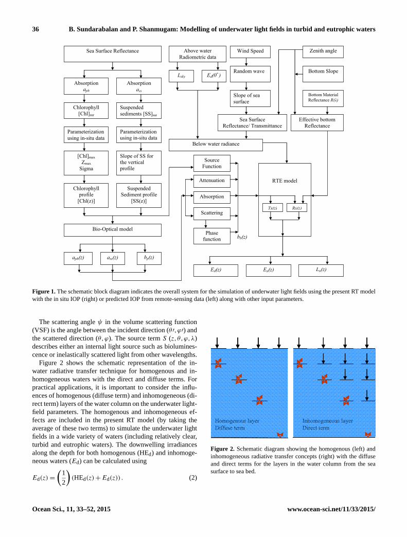
Figure 1 shows the schematic flow diagram of the present
RT model. It can simulate the underwater light fields based
on the measured IOPs (right part) or predicted IOPs from the
remote-sensing data (left part) for the same solar incident ge-
ometry and surface and bottom boundary conditions. For the
second part, surface Chl and SS are estimated from remote-
sensing reflectance data and their vertical profiles are subse-
quently predicted using the known functions. These vertical
profiles are used to derive the IOPs (hereafter referred to as
Pred IOP). Finally, the Pred IOPs are used along with the
other input parameters to simulate the underwater light fields.
The step-by-step procedure is detailed in what follows.
3.1 Radiative transfer model
Radiative transfer is the physical phenomenon of energy
transfer in the form of electromagnetic radiation. The propa-
gation of radiation through a medium is affected by absorp-
tion, emission and scattering processes. The equation of ra-
diative transfer describes these interactions mathematically.
The basic RT equation that connects the radiance and IOPs
is expressed as follows:
cosθdL(z,θ,φ,λ)
dz=−c(z,λ)L(z,θ,φ,λ)
+
∫4π
L(z,θ ′,φ′,λ)
×β(z;θ ′,φ′→ θ,φ;λ)d�′
+ S(z,θ,φ,λ). (1)
www.ocean-sci.net/11/33/2015/ Ocean Sci., 11, 33–52, 2015
36 B. Sundarabalan and P. Shanmugam: Modelling of underwater light fields in turbid and eutrophic waters
Sea Surface Reflectance
Absorption ass
Suspended sediments [SS]sur
Absorption aph
Chlorophyll [Chl]sur
Parameterization using in-situ data
Parameterization using in-situ data
Slope of SS for the vertical profile
[Chl]max Zmax
Sigma
Suspended Sediment profile
[SS(z)]
Chlorophyll profile
[Chl(z)]
bp(z) ass(z)
Bio-Optical model
aph(z)
Lu(z) Eu(z) Ed(z)
RTE model
Ed(0+)
Zenith angle Wind Speed
Lsky
Absorption
Phase function
Attenuation
Scattering
Bottom Material Reflectance R(λ)
Random wave
Slope of sea surface
Sea Surface Reflectance/ Transmittance
Bottom Slope
Effective bottom Reflectance
Above water Radiometric data
Below water radiance
Source Function
bb(z)
Tx(z) Rx(z)
Figure 1. The schematic block diagram indicates the overall system for the simulation of underwater light fields using the present RT model
with the in situ IOP (right) or predicted IOP from remote-sensing data (left) along with other input parameters.
The scattering angle ψ in the volume scattering function
(VSF) is the angle between the incident direction (θ ′,ϕ′) and
the scattered direction (θ,ϕ). The source term S (z,θ,ϕ,λ)
describes either an internal light source such as biolumines-
cence or inelastically scattered light from other wavelengths.
Figure 2 shows the schematic representation of the in-
water radiative transfer technique for homogenous and in-
homogeneous waters with the direct and diffuse terms. For
practical applications, it is important to consider the influ-
ences of homogenous (diffuse term) and inhomogeneous (di-
rect term) layers of the water column on the underwater light-
field parameters. The homogenous and inhomogeneous ef-
fects are included in the present RT model (by taking the
average of these two terms) to simulate the underwater light
fields in a wide variety of waters (including relatively clear,
turbid and eutrophic waters). The downwelling irradiances
along the depth for both homogenous (HEd) and inhomoge-
neous waters (Ed) can be calculated using
Ed(z)=
(1
2
)(HEd(z)+Ed(z)) . (2)
Homogenous layer Diffuse term
Inhomogeneous layer Direct term
Homogenous layer Diffuse term
Inhomogeneous layer Direct term
Figure 2. Schematic diagram showing the homogenous (left) and
inhomogeneous radiative transfer concepts (right) with the diffuse
and direct terms for the layers in the water column from the sea
surface to sea bed.
Ocean Sci., 11, 33–52, 2015 www.ocean-sci.net/11/33/2015/
B. Sundarabalan and P. Shanmugam: Modelling of underwater light fields in turbid and eutrophic waters 37
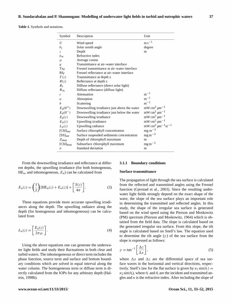
Table 1. Symbols and notations.
Symbol Description Unit
U Wind speed m s−1
θz Solar zenith angle degree
z Depth m
nw Refractive index
µ Average cosine
q Transmittance at air–water interface
TxF Fresnel transmittance at air–water interface
RfF Fresnel reflectance at air–water interface
T (z) Transmittance at depth z
R(z) Reflectance at depth z
Rs Diffuse reflectance (direct solar light)
R∞ Diffuse reflectance (diffuse light)
c Attenuation m−1
a Absorption m−1
b Scattering m−1
Ed(0+) Downwelling irradiance just above the water mW cm2 µm−1
Ed(0−) Downwelling irradiance just below the water mW cm2 µm−1
Ed(z) Downwelling irradiance mW cm2 µm−1
Eu(z) Upwelling irradiance mW cm2 µm−1
Lu(z) Upwelling radiance mW cm2 µm−1sr−1
[Chl]sur Surface chlorophyll concentration mg m−3
[SS]sur Surface suspended sediments concentration mg m−3
Zmax Depth of chlorophyll maximum m
[Chl]max Subsurface chlorophyll maximum mg m−3
σ Standard deviation m
From the downwelling irradiance and reflectance at differ-
ent depths, the upwelling irradiance (for both homogenous,
HEu, and inhomogeneous, Eu) can be calculated from
Eu(z)=
(1
2
)[HEu(z)+Eu(z)]+
[S(z)
4π
]. (3)
These equations provide more accurate upwelling irradi-
ances along the depth. The upwelling radiance along the
depth (for homogenous and inhomogeneous) can be calcu-
lated from
Lu(z)=
[Eu(z)
2πµ
]. (4)
Using the above equations one can generate the underwa-
ter light fields and study their fluctuations in both clear and
turbid waters. The inhomogeneous or direct term includes the
phase function, source term and surface and bottom bound-
ary conditions which are solved in equal interval along the
water column. The homogeneous term or diffuse term is di-
rectly calculated from the IOPs for any arbitrary depth (Hal-
trin, 1998b).
3.1.1 Boundary conditions
Surface transmittance
The propagation of light through the sea surface is calculated
from the reflected and transmitted angles using the Fresnel
function (Gjerstad et al., 2003). Since the resulting under-
water light fields strongly depend on the exact shape of the
wave, the slope of the sea surface plays an important role
in determining the transmitted and reflected angles. In this
study, the shape of the irregular sea surface is generated
based on the wind speed using the Pierson and Moskowitz
(PM) spectrum (Pierson and Moskowitz, 1964) which is ob-
tained from the field data. The slope is calculated based on
the generated irregular sea surface. From this slope, the tilt
angle is calculated based on Snell’s law. The equation used
to determine the tilt angle (γ ) of the sea surface from the
slope is expressed as follows:
γ = tan−1
[1z
1x
], (5)
where 1x and 1z are the differential space of sea sur-
face waves in the horizontal and vertical directions, respec-
tively. Snell’s law for the flat surface is given by n1 sin(θi)=
n2 sin(θt), where θi and θt are the incident and transmitted an-
gles and n is the refractive index. After including the slope of
www.ocean-sci.net/11/33/2015/ Ocean Sci., 11, 33–52, 2015
38 B. Sundarabalan and P. Shanmugam: Modelling of underwater light fields in turbid and eutrophic waters
the titled angle in the above equation, the transmitted angle
for the sea surface is calculated from
θt = sin−1
[n1
n2
sin(θi + γ )
]− γ. (6)
The modified transmitted and incident angles are applied
in the Fresnel equation as follows:
RfF =1
2
[(sin(θi − θt)
sin(θi + θt)
)2
+
(tan(θi − θt)
tan(θi + θt)
)2], θi 6= θt
=
(nw− 1
nw+ 1
)2
, θi = θt
TxF = 1−RfF. (7)
The transmittance calculated from the above equation is used
as the interface between the air and water for the down-
welling irradiance (notations given in Table 1).
Bottom reflectance
The effective reflectance Reff of the bottom (considering the
bottom material and morphology) is calculated according to
Zaneveld and Boss (2003):
Reff(λ)
Rb(λ)= 0.5× cos[θz+ θb] + 0.5× cos[θz− θb], (8)
where θb = a tan(4Ab/Lb) the angle of the bottom slope (due
to ripples on the sea bed), and θz is the zenith angle of the
irradiance. Ab and Lb are the amplitude and wavelength, re-
spectively, for the triangular shaped bottom. The effective re-
flectance spectra of the sea bottom are not same for different
materials since the reflectance is about to vary for different
materials.
3.1.2 Optical properties in the water column
Phase function
The angular distributions of scattered radiance are mainly ex-
plained in terms of the phase function, which plays an im-
portant role in coastal waters. The characteristic of phase
functions in natural volumetric media is sharply peaked in
the forward scattering direction, with only a few percent of
backscatter in the total angular redistribution of a single scat-
tering event (Sundarabalan et al., 2013). Of several phase
function models developed in the past, the Fournier–Forand
(FF) model is an analytic form of the phase function giving
better results when compared to other models (Mobley et al.,
2002). The FF phase function is given by
β(θ)=1
4π(1− δ)2δv
{ [v(1− δ)− (1− δv)
]+
[δ(1− δv)− v(1− δ)sin−2
(θ
2
)]}
+1− δv180
16π(δ180− 1)δv180
(3cos2θ − 1
)v =
3−µ
2, δ =
4
3(n− 1)2sin2
(θ
2
). (9)
Here µ is the slope of the Junge particle distribution, n is
the real index of refraction and δ180 is calculated by consider-
ing θ = 180◦. Based on previous studies (Twardowski et al.,
2001; Freda and Piskozub, 2007; Sundarabalan et al., 2013),
the parameters µ and n are modelled using the IOPs, atten-
uation c(520) and scattering b(520). Finally, the backscatter-
ing bb coefficients are computed from the phase function for
scattering angles between 90 and 180◦,
bb(520)=
π∫π2
β(θ)dθ. (10)
The spectral variation of the backscattering bb coefficients
can be expressed as (Haltrin, 2002)
bb(λ)= bb(520)×
(520
λ
)1.1
. (11)
This phase function is mainly used to determine the bb
coefficients along the depth, which are more compatible for
turbid coastal waters.
Transmittance along the depth
Haltrin (1998b) derived the transmittance as a function of
depth T (z) based on the self-consistent method, which de-
pends on the IOPs of seawater. The transmittance function
T (z) is expressed as
T (z)=1+ q {µsε(z)+hRsFs(z)[(2+µ)µs+ 1]}
1+ qµs
. (12)
Several important parameters that depend on the IOPs are
used to calculate T (z). µs is the cosine function related to the
solar angle which is calculated based on the refractive index
of seawater (n) and the solar elevation hs. µ is the average
cosine that connects with Gordon’s parameter g, which de-
pends on the absorption and backscattering coefficients. The
result obtained by solving the RT equation is α∞ which is
found by dividing absorption (a) by the average cosine (µ).
µ0 is another cosine function which depends on the average
cosine µ. The reflectance parameters involved in the calcu-
lation of T (z) are the diffuse reflectance (Rs) of a deep sea
layer optically illuminated by direct solar light and the dif-
fuse reflectance (R∞) of the optically deep sea illuminated
by the diffuse light. Both are calculated as a function of the
cosine functions as follows:
Rs =(1−µ)2
1+µµs(4−µ2), R∞ =
(1−µ
1+µ
)2
. (13)
Ocean Sci., 11, 33–52, 2015 www.ocean-sci.net/11/33/2015/
B. Sundarabalan and P. Shanmugam: Modelling of underwater light fields in turbid and eutrophic waters 39
The average cosine function used in the above equation is
defined as
µ=
{1− g
1+ 2g+ [g(4+ 5g)]1/2
}1/2
,
µ0 =1+µ2
µ(3−µ2),
µs =
[1−
(coshs
nw
)2]1/2
, (14)
where c = a+ b is the beam attenuation coefficient, q =E⊥sE0
d
is the transmittance at air–sea interface, α = a+ 2bb is the
re-normalised attenuation coefficient, α∞ =aµ
is the inter-
mediate parameter which depends on IOPs and g =bb
a+bbis
the Gordon’s parameter (Gordon et al., 1975; Haltrin, 2003)
which depends on absorption and scattering.
The IOP-dependent intermediate parameters are defined as
ε(z)= exp
[−αz
(1
µs
−1
µ0
)], h=
(1+µ)2
2(1+µ2),
Fs(z)=
(1− exp
[−αz
(1
µs
−1
µ0
)])/(1
µs
−1
µ0
),
µs 6= µ0,
Fs(z)= αz, µs = µ0. (15)
The above parameters, ε(z), h, and Fs(z), are the func-
tions calculated based on the IOPs and solar elevation (Hal-
trin, 1998b).
Reflectance along the depth
The reflectance along the depth R(z) is generally calculated
based on the IOPs (bb/(a+ bb)), but it is also highly influ-
enced by the bottom material and solar zenith angle (Lee et
al., 1998, 1999). Thus, the reflectance along the depth is cal-
culated from Lee et al. (1998), which takes into account the
bottom material effect and the IOPs of the water column. The
model parameters are defined as follows:
R(z)= Riop(z)+Rbtm(z). (16)
The reflectance influenced by the IOPs and bottom effect
are calculated from the following equations:
Riop(z)=
rrs(z)×
{1− exp
[−κ(z)H
(Dc
u+
(1
cosθw
))]},
Rbtm(z)=
Reffbtm×
{−exp
[−κ(z)H
(Db
u(z)+
(1
cosθw
))]}, (17)
where Dcu is the path-elongation factor for scattered photons
from the water column which varies with the IOPs. The opti-
cal path-elongation factorDbu for the bottom mainly depends
on the bottom reflectance. These factors are defined as
Dcu = 1.03
√(1+ (2.4× u)), (18)
Dbu = 1.04
√(1+ (5.4× u)). (19)
rrs is the subsurface remote-sensing reflectance which is a
function of the IOPs at a given depth and expressed as
rrs = u× [(u× 0.170)+ 0.084] . (20)
Also, θw is the subsurface solar zenith angle, H is the bot-
tom depth, Reffbtm is the effective bottom reflectance and κ
and u are the inherent optical parameters which can be ob-
tained from
u=bb(z)
a(z)+ bb(z), (21)
κ = a(z)+ bb(z). (22)
Based on the IOPs along the depth and effective re-
flectance of the bottom, the reflectance functions along the
depth R(z) can be calculated from these equations.
Source function
Since the source function affects the underwater light fields
(by way of re-emitting photons by phytoplankton at longer
wavelengths after absorption at shorter wavelengths), it is
also included in the present RT model. The source function
can be computed as follows (Gower et al., 2004):
Fl(λ)=0.15×Chl
1+ 0.2×Chl. (23)
The source function is calculated as a function of the
chlorophyll fluorescence as follows:
S(λ)= Fl(λ)×h(λ), (24)
where h(λ) is the fluorescence emission function per unit
wavelength calculated based on the Gaussian distribution,
h(λ)=1
√2πσ 2
exp
(−(λ− λ0)
2
2σ 2
). (25)
The wavelength of maximum emission is λ0 = 0.685 µm
and the standard deviation σ = 0.011 µm.
3.1.3 Inhomogeneous term: underwater light-field
parameters
The downwelling irradiance Ed(0−) just below the water for
the inhomogeneous (or layer by layer) condition can be cal-
culated from the downwelling irradiance Ed(0+) just above
the water along with the transmittance derived from the Fres-
nel equation (Eq. 7),
Ed(0−)= Ed(0
+)×TxF. (26)
www.ocean-sci.net/11/33/2015/ Ocean Sci., 11, 33–52, 2015
40 B. Sundarabalan and P. Shanmugam: Modelling of underwater light fields in turbid and eutrophic waters
Once the downwelling irradiance is transmitted through
the water surface, the intensity of the downwelling irradiance
based on the transmittance is purely dependent on the IOPs.
The downwelling irradiances for the first and subsequent lay-
ers of the depth are calculated from
Ed(z1)= Ed(0−);Ed(z2)= Ed(z1)×Tx(z2). (27)
The downwelling irradiance along the depth can be calcu-
lated from an explicit method with the corresponding depth
transmittance Tx(z). The common equation for calculating
Ed(z) along the depth is given as
Ed(z)= Ed(z− 1)×Tx(z). (28)
The upwelling irradiances below the water along the depth
are calculated from
Eu(z)= (Ed(z)×R(z)) , (29)
where Ed(z) is downwelling irradiance and R(z) is the re-
flectance for the corresponding depth which includes the ef-
fect of the bottom reflectance and IOPs from the bottom
boundary condition.
3.1.4 Homogeneous term: underwater light-field
parameters
The downwelling irradiance equation developed by Hal-
trin (1998b) for the homogenous water column takes the fol-
lowing expression,
HEd(z)= E0d exp(−α∞z)+E
⊥s exp(−αz/µs) (30)
+E⊥s hRs {1+µs(2+µ)}Fs(z)exp(−α∞z). (31)
The upwelling irradiance for the homogenous water col-
umn can be calculated with the equation of Haltrin (1998b):
HEu(z)=
E0dR∞ exp(−α∞z)+µsE
⊥s R∞ exp(−αz/µs) (32)
+E⊥s hRs {µs(2−µ)− 1}Fs(z)exp(−α∞z). (33)
The input parameters used in the calculation of HEd and
HEu are explained in the transmittance section. Here, Es is
the diffuse term of the above-water irradiance which is ob-
tained from the sky radianceLsky. The total underwater light-
field parameters (Ed,Eu andLu) can be obtained by applying
Eqs. (26)–(29) in Eqs. (2)–(4). The model presented in this
study is much easier to implement when compared to the ex-
isting RT models.
3.2 Prediction of remotely sensed IOPs along the water
column
3.2.1 Bio-optical model
This section presents methods to estimate the surface chloro-
phyll [Chl]sur and suspended sediments [SS]sur (concentra-
tions) from the normalised water-leaving radiance (nLw).
The slope values (SnLw) required for fixing the threshold
limit (i.e., scenarios in Table 3) for different waters are cal-
culated as follows:
SnLw = 100×
[nLw(0.443)− nLw(0.547)
0.443− 0.547
]. (34)
Since the normalised water-leaving radiance values are
larger than the remote-sensing reflectance, the former quan-
tity is used to better determine the used scenarios (Ahn and
Shanmugam, 2006; Shanmugam, 2011b). Based on the SnLw
and nLw data, three scenarios are found adequate for the vari-
ous water types. The first scenario represents the open-ocean
waters where SnLw is less than 0.5 and [Chl] is based on the
ratio of Rrs (0.488) and Rrs (0.547) (Table 3). The second
scenario indicates turbid coastal waters where the same band
ratio is used for the [Chl] parameterisation. The [SS] param-
eterisations are different for both these scenarios. The third
scenario is developed for inland and eutrophic waters based
on the exponential function that uses the Rrs values at three
different bands (0.690, 0.700 and 0.760 µm) (Zhang et al.,
2009). The coefficients of the exponential equation are ob-
tained based on the IRrs value which is defined as follows:
IRrs =
(1
Rrs(0.690)−
1
Rrs(0.700)
)×Rrs(0.760). (35)
For the [SS] parameterisation, there is a shift of peak be-
tween 0.547 and 0.488 µm in clear waters (first scenario) and
the ratio of Rrs (0.620) to the maximum value of Rrs (0.488)
and Rrs (0.547) is found to be suitable for these waters. In
turbid coastal waters (second scenario), the reflectance peak
at 0.547 µm dominates the Rrs values at 0.488 µm and the rel-
ative change of these values is used in terms of the ratio to
estimate [SS] in turbid waters. Considering inland and eu-
trophic waters (third scenario), the ratio of Rrs at 0.620 and
0.720 µm is used for the estimation of [SS] in these waters.
3.2.2 Vertical profiles of chlorophyll and suspended
sediments
The chlorophyll and suspended sediments along the verti-
cal column are determined from the surface [Chl] and [SS]
data. For the chlorophyll profile, Lewis et el. (1983) found
the generalised Gaussian distribution model which captures
the major features of the observed vertical profile. The major
parameters used to determine the chlorophyll profile are the
surface chlorophyll [Chl]sur, maximum chlorophyll [Chl]max,
depth chlorophyll maximum Zmax and σ (standard deviation
that controls the thickness of the [Chl]max layer and deter-
mines the vertical spread). The [Chl]max is the value of max-
imum chlorophyll in the water column and Zmax is the depth
of [Chl]max. The schematic representation of these chloro-
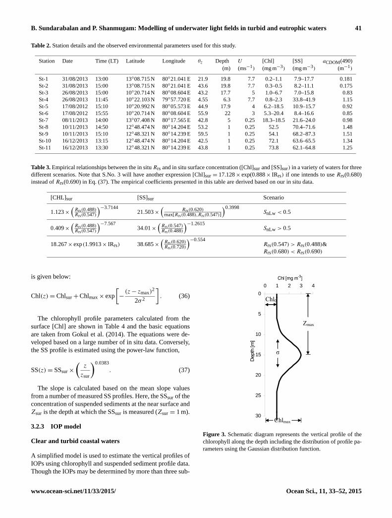
phyll profile parameters is shown in Fig. 3. The determina-
tion of the chlorophyll profile based on the above parameters
Ocean Sci., 11, 33–52, 2015 www.ocean-sci.net/11/33/2015/
B. Sundarabalan and P. Shanmugam: Modelling of underwater light fields in turbid and eutrophic waters 41
Table 2. Station details and the observed environmental parameters used for this study.
Station Date Time (LT) Latitude Longitude θz Depth U [Chl] [SS] aCDOM(490)
(m) (ms−1) (mg m−3) (mg m−3) (m−1)
St-1 31/08/2013 13:00 13◦08.715 N 80◦21.041 E 21.9 19.8 7.7 0.2–1.1 7.9–17.7 0.181
St-2 31/08/2013 15:00 13◦08.715 N 80◦21.041 E 43.6 19.8 7.7 0.3–0.5 8.2–11.1 0.175
St-3 26/08/2013 15:00 10◦20.714 N 80◦08.604 E 43.2 17.7 5 1.0–6.7 7.0–15.8 0.83
St-4 26/08/2013 11:45 10◦22.103 N 79◦57.720 E 4.55 6.3 7.7 0.8–2.3 33.8–41.9 1.15
St-5 17/08/2012 15:10 10◦20.992 N 80◦05.573 E 44.9 17.9 4 6.2–18.5 10.9–15.7 0.92
St-6 17/08/2012 15:55 10◦20.714 N 80◦08.604 E 55.9 22 3 5.3–20.4 8.4–16.6 0.85
St-7 08/11/2013 14:00 13◦07.408 N 80◦17.565 E 42.8 5 0.25 18.3–18.5 21.6–24.0 0.98
St-8 10/11/2013 14:50 12◦48.474 N 80◦14.204 E 53.2 1 0.25 52.5 70.4–71.6 1.48
St-9 10/11/2013 15:10 12◦48.321 N 80◦14.239 E 59.5 1 0.25 54.1 68.2–87.3 1.51
St-10 16/12/2013 13:15 12◦48.474 N 80◦14.204 E 42.5 1 0.25 72.1 63.6–65.5 1.34
St-11 16/12/2013 13:30 12◦48.321 N 80◦14.239 E 43.8 1 0.25 73.8 62.1–64.8 1.25
Table 3. Empirical relationships between the in situ Rrs and in situ surface concentration ([Chl]sur and [SS]sur) in a variety of waters for three
different scenarios. Note that S.No. 3 will have another expression [Chl]sur = 17.128× exp(0.888× IRrs) if one intends to use Rrs(0.680)
instead of Rrs(0.690) in Eq. (37). The empirical coefficients presented in this table are derived based on our in situ data.
[CHL]sur [SS]sur Scenario
1.123×(Rrs(0.488)Rrs(0.547)
)−3.714421.503×
(Rrs(0.620)
max[Rrs(0.488),Rrs(0.547)]
)0.3998SnLw < 0.5
0.409×(Rrs(0.488)Rrs(0.547)
)−7.56734.01×
(Rrs(0.547)Rrs(0.488)
)−1.2615SnLw > 0.5
18.267× exp(1.9913× IRrs) 38.685×(Rrs(0.620)Rrs(0.720)
)−0.554Rrs(0.547) > Rrs(0.488)&
Rrs(0.680) < Rrs(0.690)
is given below:
Chl(z)= Chlsur+Chlmax× exp
[−(z− zmax)
2
2σ 2
]. (36)
The chlorophyll profile parameters calculated from the
surface [Chl] are shown in Table 4 and the basic equations
are taken from Gokul et al. (2014). The equations were de-
veloped based on a large number of in situ data. Conversely,
the SS profile is estimated using the power-law function,
SS(z)= SSsur×
(z
zsur
)0.0383
. (37)
The slope is calculated based on the mean slope values
from a number of measured SS profiles. Here, the SSsur of the
concentration of suspended sediments at the near surface and
Zsur is the depth at which the SSsur is measured (Zsur = 1 m).
3.2.3 IOP model
Clear and turbid coastal waters
A simplified model is used to estimate the vertical profiles of
IOPs using chlorophyll and suspended sediment profile data.
Though the IOPs may be determined by more than three sub-
0
5
10
15
20
25
30
0 1 2 3 4
σ
Dep
th [m
]
Chl [mg m-3]
Zmax
Chlmax
Chl0
Figure 3. Schematic diagram represents the vertical profile of the
chlorophyll along the depth including the distribution of profile pa-
rameters using the Gaussian distribution function.
www.ocean-sci.net/11/33/2015/ Ocean Sci., 11, 33–52, 2015
42 B. Sundarabalan and P. Shanmugam: Modelling of underwater light fields in turbid and eutrophic waters
Table 4. Empirical relationships of the chlorophyll profile parameters ([Chl]max, Zmax and σ) for the various ranges of surface chlorophyll
[Chl]sur from different stations.
Chlsur Chlmax Zmax 6
1.0<Chlsur< 10 2.019×Chlsur− 0.2328 0.7595×Chlsur+ 4.082 0.3456×Chlsur+ 4.104
0.5<Chlsur< 1 −8.288×Chlsur+ 8.3628 −12.247×Chlsur+ 15.479 3.1606×Chlsur− 0.199
0<Chlsur< 0.5 −8.288×Chlsur+ 2.6628 −12.247×Chlsur+ 15.479 3.1606×Chlsur− 0.199
stances, it is assumed that the absorption and scattering co-
efficients in clear and turbid coastal waters are mainly de-
termined by water itself, suspended sediment particles and
phytoplankton (both living and non-living). Thus, the to-
tal absorption coefficient of seawater, a(λ, z), is the sum
of the absorption of seawater aw(λ, z), dissolved organic
aCDOM(λ,z), and particulate matter ap(λ, z). The total ab-
sorption coefficient observed at any given wavelength can be
expressed as
a(λ,z)= aw(λ,z)+ aCDOM(λ,z)+ ap(λ,z), (38)
ap(λ,z)= aph(λ,z)+ ass(λ,z). (39)
Here the total absorption (pure water, chlorophyll, sus-
pended sediments and coloured dissolved organic matter)
is estimated from Morel (1991) and the absorption coeffi-
cient of suspended sediments is calculated from Gokul et
al. (2014):
a(λ,z)=(aw(λ)+ 0.06a∗C(λ)[Chl(z)]0.65
)×
(1+ 0.2exp(−0.014(λ− 0.400)× 10−3)
)+ ass(λ,z). (40)
The seawater absorption coefficients were taken from Pope
and Fry (1997). The absorption coefficient of suspended sed-
iments is estimated as follows:
ass(λ,z)= ass(λr)× exp(−0.0104(λ− λr)), (41)
where the absorption at a reference wavelength 0.443 µm is
calculated from the power fit shown in Fig. 4a and the equa-
tion is given as
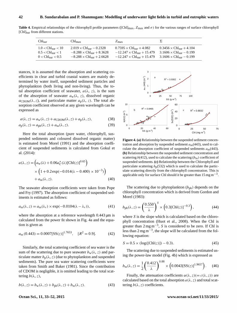
ass (0.443)= 0.0007[SS(z)]1.7653, [R2= 0.9]. (42)
Similarly, the total scattering coefficient of sea water is the
sum of the scattering due to pure seawater bw(λ, z) and par-
ticulate matter bp(λ, z) (due to phytoplankton and suspended
sediments). The pure sea water scattering coefficients were
taken from Smith and Baker (1981). Since the contribution
of CDOM is negligible, it is omitted leading to the total scat-
tering b(λ, z),
b(λ,z)= bw(λ,z)+ bph(λ,z)+ bss(λ,z). (43)
R2 = 0.8465
0
5
10
0 20 40 60SS (g m-3)
b(41
2) (
m-1
) R2 = 0.8832
0
20
40
60
0 25 50 75
Chl (mg m-3)
bp(5
32
) (m
-1)
R2 = 0.9302
0
1
2
3
0 25 50 75 100
SS (g m-3)
ass
(443
) (m
-1) a
b c
Figure 4. (a) Relationship between the suspended sediment concen-
tration and absorption by suspended sediment ass(443), used to cal-
culate the absorption coefficient of suspended sediments ass(443).
(b) Relationship between the suspended sediment concentration and
scattering b(412), used to calculate the scattering (bss) coefficient of
suspended sediments. (c) Relationship between the Chlorophyll and
particulate scattering bp(532) which is used to calculate the partic-
ulate scattering directly from the chlorophyll concentration. This is
applicable only for surface Chl should it be greater than 15 mg m−3.
The scattering due to phytoplankton (bph) depends on the
chlorophyll concentration which is derived from Gordon and
Morel (1983):
bph(λ,z)=
(0.550
λ
)S×
(0.3[Chl(z)]−0.3
), (44)
where S is the slope which is calculated based on the chloro-
phyll concentration (Huot et al., 2008). When the Chl is
greater than 2 mg m−3, S is considered to be zero. If Chl is
less than 2 mg m−3, the slope will be calculated from the fol-
lowing equation:
S = 0.5× (log([Chl(z)])− 0.3). (45)
The scattering due to suspended sediments is estimated us-
ing the power-law model (Fig. 4b) which is expressed as
bss(λ,z)=1
2
(0.412
λ
)0.88
×
(0.0043[SS(z)]1.9657
). (46)
Finally, the attenuation coefficients α(λ,z)(= c(λ,z)) are
calculated based on the total absorption a(λ,z) and total scat-
tering b(λ,z) coefficients.
Ocean Sci., 11, 33–52, 2015 www.ocean-sci.net/11/33/2015/
B. Sundarabalan and P. Shanmugam: Modelling of underwater light fields in turbid and eutrophic waters 43
Table 5. New spectral absorption coefficients of water particles de-
rived from the in situ data, which are used only when the concen-
tration of [Chl]sur is greater than 15 mg m−3, for the calculation of
the particulate absorption.
Wavelength a∗p Wavelength a∗p(µm) (µm)
0.401 0.195342 0.575 0.038799
0.425 0.208779 0.601 0.044386
0.451 0.168103 0.625 0.056005
0.475 0.129094 0.651 0.053105
0.501 0.098007 0.675 0.080339
0.525 0.061625 0.701 0.019868
0.551 0.042149 0.725 0.002783
Eutrophic and phytoplankton-dominated waters
For eutrophic and phytoplankton-dominated waters, the vari-
ations in absorption and scattering coefficients are poorly
documented as most of the previous studies on IOPs were
conducted in relatively clear and open-ocean waters. In this
study, absorption and scattering by particles are estimated us-
ing separate models for these waters. In the previous studies,
phytoplankton absorption aph(λ) was generally calculated
based on the specific phytoplankton absorption a∗ph(λ). Here
the specific particulate absorption coefficients a∗p(λ) are used
to calculate the particulate absorption coefficients ap(λ). The
values of new a∗p(λ) are given in Table 5. The particulate ab-
sorption coefficients are then derived as a function of chloro-
phyll as follows:
ap(λ,z)= a∗p(λ)×[Chl(z)]×
([Chl(z)]
54
). (47)
Similarly, the particulate scattering is calculated directly
based on the exponential function of chlorophyll (Fig. 4c) as
follows:
bp(λ,z)=
1.4× exp(0.0525×[Chl(z)])×
(λ
0.532
)−0.3
. (48)
This equation is derived from the relationship between in
situ chlorophyll and particulate scattering (c–a from Wet-
Labs AC-S). Both particulate absorption and scattering coef-
ficients are added with the respective pure water coefficients
to obtain the total absorption and scattering coefficients.
4 Results and discussion
Results are categorised into four parts: (1) comparison of
the model versus measured IOP profile data, (2) effects of
homogeneous and inhomogeneous water column conditions,
(3) comparison of the underwater light fields predicted by the
400 500 600 7000
2
4
6
8x 10
-3
Wavelength (x10-3 m) Wavelength (x10-3 m)
Rrs
Rrs
400 500 600 7000
0.005
0.01
400 500 600 7000
0.005
0.01
0.015
0.02
400 500 600 7000
0.01
0.02
0.03
0.04
a b
d c
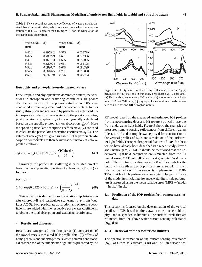
Figure 5. The typical remote-sensing reflectance spectra Rrs(λ)
measured at four stations in the study area during 2012 and 2013.
(a) Relatively clear waters off Chennai, (b) moderately turbid wa-
ters off Point Calimere, (c) phytoplankton-dominated harbour wa-
ters of Chennai and (d) eutrophic waters.
RT model, based on the measured and estimated IOP profiles
from remote-sensing data, and (4) apparent optical properties
from underwater light fields. Figure 5 shows the examples of
measured remote-sensing reflectances from different waters
(clear, turbid and eutrophic waters) used for construction of
the vertical profiles of IOPs and simulation of the underwa-
ter light fields. The specific spectral features of IOPs for these
waters have already been described in a recent study (Pravin
and Shanmugam, 2014). It should be mentioned that the un-
derwater light-field parameters are simulated from the RT
model using MATLAB 2007 with a 4 gigabyte RAM com-
puter. The run time for this model is 8 milliseconds for the
entire wavelength at one depth for a given sample. In fact,
this can be reduced if the model is implemented in FOR-
TRAN with a high performance computer. The performance
of the model in simulating the underwater light-field parame-
ters is assessed using the mean relative error (MRE =(model
− in situ)/in situ).
4.1 Prediction of the IOP profiles from remote-sensing
data
This section is focused on the determination of the vertical
profiles of IOPs based on the seawater constituents (chloro-
phyll and suspended sediments at the surface level) that are
estimated from the above-water remote-sensing reflectance
(Rrs) data.
4.1.1 Retrieval of the seawater constituents
The spectral information of the remote-sensing reflectance
(Rrs) was used to estimate [Chl] and [SS] in surface wa-
www.ocean-sci.net/11/33/2015/ Ocean Sci., 11, 33–52, 2015
44 B. Sundarabalan and P. Shanmugam: Modelling of underwater light fields in turbid and eutrophic waters
0.1 1 10 100 5000.1
1
10
100
500
Insitu - Chl [mg m-3]
Mod
el -
Chl
[mg
m-3
]
0 25 50 75 1000
25
50
75
100
Insitu - SS [mg m-3]M
odel
- S
S [m
g m
-3]
a b
Figure 6. (a) Scatter plot showing the comparison of the estimated
chlorophyll concentration from the remote-sensing reflectance Rrs
with the in situ chlorophyll from different waters. (b) Scatter plot
showing the comparison of the estimated suspended sediment con-
centration from the remote-sensing reflectance Rrs with the in situ
suspended sediment concentration from different waters.
ters off Point Calimere and Chennai. Since the models are
based on the different spectral slopes of Rrs, different sce-
narios were used to estimate these water constituents ac-
curately. The estimated [Chl] and [SS] show good agree-
ment with measured data from different waters (Fig. 6a),
where [Chl] ranged from 0.1 to 100 mg m−3. The statis-
tics analyses indicate low errors and high slopes and corre-
lation coefficients (MRE= 0.17, RMSE= 0.18, slope= 1.0,
bias=−0.031, R2= 0.91, N= 98). Similarly, the estimated
[SS] agree closely with the in situ [SS] (Fig. 6b), with
good statistics (MRE= 0.01, RMSE= 0.09, slope= 0.98,
bias=−0.01, R2= 0.84, N = 98). These results clearly
demonstrate consistency between the estimated and mea-
sured data for a wide range of waters.
4.1.2 Vertical profiles of chlorophyll and suspended
sediments
On the basis of surface chlorophyll [Chl]surf and [SS] es-
timated from remote-sensing data, the vertical profiles of
[Chl(z)] and [SS(z)] were constructed in relatively clear and
turbid coastal waters. It is observed that the modelled and
measured chlorophyll profiles agree well in relatively clear
waters off Chennai (31 August 2013 at 13:00 and 15:00 LT)
(Fig. 7a and b). The Chl concentration is low in surface wa-
ters (0.3 mg m−3) and gradually increases along the depth.
For relatively clear waters off Point Calimere in August 2013
(Fig. 7c), the surface chlorophyll is very low (0.8 mg m−3)
and the depth of chlorophyll maximum (Zmax) shifts to the
seabed exponentially. This profile is the indication of more
light attenuation towards the sea bed. The subsurface chloro-
phyll maximum [Chl]max might occur due to the influences
of benthic resuspension caused by tides and currents. Though
the modelled chlorophyll profile typically follows the mea-
sured chlorophyll profile at this station, there is a slight de-
viation of the modelled chlorophyll profile observed at the
intermediate depth. The [Chl]surf in surface waters off Point
Calimere is relatively high (5 mg m−3) during August 2012
0 10 20
0
5
10
15
200 10 20
0
5
10
15
200 20 40
0
5
10
15
200 20 40
0
5
10
15
200 20 40
0
5
10
15
20
Dep
th [m
]
SS [mg m-3] SS [mg m-3] SS [mg m-3] SS [mg m-3] SS [mg m-3]
0 2 4
0
5
10
15
200 2 4
0
5
10
15
200 5 10
0
5
10
15
200 10 20 30
0
5
10
15
200 10 20 30
0
5
10
15
20
Dep
th [m
]
Chl [mg m-3] Chl [mg m-3] Chl [mg m-3] Chl [mg m-3] Chl [mg m-3]
a b c d e
In-situ Model
In-situModel
Figure 7. The examples of the modelled and measured vertical pro-
files of [Chl(z)] for five different cases (top row). (a and b) St-1 and
St-2 from relatively clear waters off Chennai, (c) St-4 from moder-
ately turbid water with chlorophyll settled at the bottom of seabed.
(d and e) St-6 and St-5 from the chlorophyll-dominated regions.
The second row shows the modelled and measured vertical profiles
of [SS(z)] for the same locations. The [SS(z)] modelled profiles are
almost uniform along the depth.
(Fig. 7d). As the depth increases, [Chl] increases with a max-
imum value ([Chl]max) around 7 m depth (20 mg m−3) and
then decreases following the surface [Chl]surf. This trend typ-
ically follows the Gaussian distribution function, and thus
there is better consistency between the modelled and mea-
sured Chl profiles (Fig. 7e). Another station towards the coast
of Point Calimere during the same period was found to have a
similar Gaussian profile indicating that the euphotic zone lies
horizontally at a depth of 7 m. The corresponding measured
and modelled SS profiles [SS(z)] are shown in Fig. 7a–c for
these stations. Generally, the measured [SS] profiles are uni-
form along the depth and the power-law function captures
their depth variations adequately.
4.1.3 Modelling of IOPs based on the Chl and SS
profiles
The [Chl(z)] and [SS(z)] profiles constructed from the mod-
els were used to estimate the IOP profiles. Figure 8 shows the
comparison of estimated (black colour) and predicted (grey
colour) IOPs (plotted for three wavelengths 0.440, 0.555 and
0.676 µm) with the in situ IOP data, where the three clusters
correspond to different waters (bottom – clear waters, middle
– turbid coastal waters, top – eutrophic waters). Since a wide
variety of waters is considered in this study, separate models
were developed to treat the different water types. In Fig. 8
Ocean Sci., 11, 33–52, 2015 www.ocean-sci.net/11/33/2015/
B. Sundarabalan and P. Shanmugam: Modelling of underwater light fields in turbid and eutrophic waters 45
0.001
0.01
0.1
1
10
0.001 0.01 0.1 1 10
Mod
el -
bb(4
40)[
m-1
]
Insitu - bb(440)[m-1]
0.001
0.01
0.1
1
10
0.001 0.01 0.1 1 10
Mod
el -
bb(5
55)[
m-1
]
Insitu - bb(555)[m-1]
0.001
0.01
0.1
1
10
0.001 0.01 0.1 1 10
Mod
el -
bb(6
76)[
m-1
]
Insitu - bb(676)[m-1]
0.01
0.1
1
10
100
0.01 0.1 1 10 100Insitu - b
p(440)[m-1]
Mod
el -
bp(4
40)[
m-1
]
0.01
0.1
1
10
100
0.01 0.1 1 10 100
Insitu - bp(555)[m-1]
Mod
el -
bp(5
55)[
m-1
]
0.01
0.1
1
10
100
0.01 0.1 1 10 100
Insitu - bp(676)[m-1]
Mod
el -
bp(6
76)[
m-1
]
0.01
0.1
1
10
100
0.01 0.1 1 10 100
Mod
el -
ap(4
40)[
m-1
]
Insitu - ap(440)[m-1]
0.001
0.01
0.1
1
10
0.001 0.1 10Insitu - a
p(676)[m-1]
Mod
el -
ap(6
76)[
m-1
]
0.001
0.01
0.1
1
10
0.001 0.01 0.1 1 10Insitu - a
p(555)[m-1]
Mod
el -
ap(5
55)[
m-1
]
-Data from clear waters -Data from turbid coastal waters -Data from eutrophic lagoon waters
Model results based on the predicted concentration data
Model results based on the measured concentration data
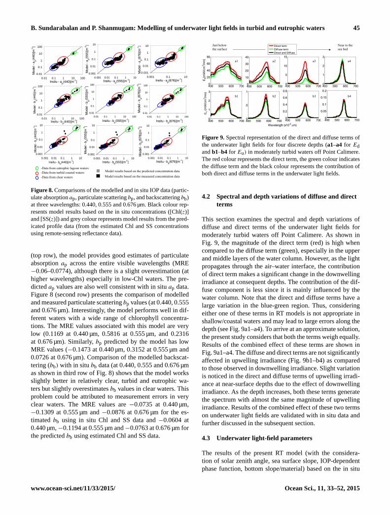
Figure 8. Comparisons of the modelled and in situ IOP data (partic-
ulate absorption ap, particulate scattering bp, and backscattering bb)
at three wavelengths: 0.440, 0.555 and 0.676 µm. Black colour rep-
resents model results based on the in situ concentrations ([Chl(z)]
and [SS(z)]) and grey colour represents model results from the pred-
icated profile data (from the estimated Chl and SS concentrations
using remote-sensing reflectance data).
(top row), the model provides good estimates of particulate
absorption ap across the entire visible wavelengths (MRE
−0.06–0.0774), although there is a slight overestimation (at
higher wavelengths) especially in low-Chl waters. The pre-
dicted ap values are also well consistent with in situ ap data.
Figure 8 (second row) presents the comparison of modelled
and measured particulate scattering bp values (at 0.440, 0.555
and 0.676 µm). Interestingly, the model performs well in dif-
ferent waters with a wide range of chlorophyll concentra-
tions. The MRE values associated with this model are very
low (0.1169 at 0.440 µm, 0.5816 at 0.555 µm, and 0.2316
at 0.676 µm). Similarly, bp predicted by the model has low
MRE values (−0.1473 at 0.440 µm, 0.3152 at 0.555 µm and
0.0726 at 0.676 µm). Comparison of the modelled backscat-
tering (bb) with in situ bb data (at 0.440, 0.555 and 0.676 µm
as shown in third row of Fig. 8) shows that the model works
slightly better in relatively clear, turbid and eutrophic wa-
ters but slightly overestimates bb values in clear waters. This
problem could be attributed to measurement errors in very
clear waters. The MRE values are −0.0735 at 0.440 µm,
−0.1309 at 0.555 µm and −0.0876 at 0.676 µm for the es-
timated bb using in situ Chl and SS data and −0.0604 at
0.440 µm,−0.1194 at 0.555 µm and−0.0763 at 0.676 µm for
the predicted bb using estimated Chl and SS data.
400 500 600 7000
1
2
3
400 500 600 7000
20
40
60
80
400 500 600 7000
10
20
30
40
400 500 600 7000
5
10
15
400 500 600 7000
0.5
1
400 500 600 7000
1
2
3
400 500 600 7000
0.2
0.4
0.6
0.8
400 500 600 7000
0.05
0.1
0.15
0.2
Just below the surface
Near to the sea bed
Wavelength (x10-3 m)
Ed(
mW
/cm
2 /m
)E
u (m
W/c
m2 /
m)
Direct termDiffuse termDirect and Diffuse
a1
b1
a2
b2
a3
b3
a4
b4
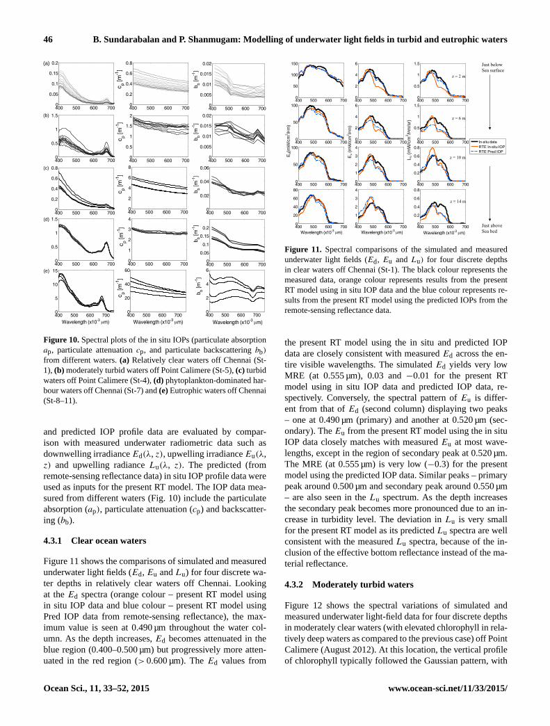
Figure 9. Spectral representation of the direct and diffuse terms of
the underwater light fields for four discrete depths (a1–a4 for Ed
and b1–b4 for Eu) in moderately turbid waters off Point Calimere.
The red colour represents the direct term, the green colour indicates
the diffuse term and the black colour represents the contribution of
both direct and diffuse terms in the underwater light fields.
4.2 Spectral and depth variations of diffuse and direct
terms
This section examines the spectral and depth variations of
diffuse and direct terms of the underwater light fields for
moderately turbid waters off Point Calimere. As shown in
Fig. 9, the magnitude of the direct term (red) is high when
compared to the diffuse term (green), especially in the upper
and middle layers of the water column. However, as the light
propagates through the air–water interface, the contribution
of direct term makes a significant change in the downwelling
irradiance at consequent depths. The contribution of the dif-
fuse component is less since it is mainly influenced by the
water column. Note that the direct and diffuse terms have a
large variation in the blue-green region. Thus, considering
either one of these terms in RT models is not appropriate in
shallow/coastal waters and may lead to large errors along the
depth (see Fig. 9a1–a4). To arrive at an approximate solution,
the present study considers that both the terms weigh equally.
Results of the combined effect of these terms are shown in
Fig. 9a1–a4. The diffuse and direct terms are not significantly
affected in upwelling irradiance (Fig. 9b1–b4) as compared
to those observed in downwelling irradiance. Slight variation
is noticed in the direct and diffuse terms of upwelling irradi-
ance at near-surface depths due to the effect of downwelling
irradiance. As the depth increases, both these terms generate
the spectrum with almost the same magnitude of upwelling
irradiance. Results of the combined effect of these two terms
on underwater light fields are validated with in situ data and
further discussed in the subsequent section.
4.3 Underwater light-field parameters
The results of the present RT model (with the considera-
tion of solar zenith angle, sea surface slope, IOP-dependent
phase function, bottom slope/material) based on the in situ
www.ocean-sci.net/11/33/2015/ Ocean Sci., 11, 33–52, 2015
46 B. Sundarabalan and P. Shanmugam: Modelling of underwater light fields in turbid and eutrophic waters
400 500 600 7000
0.05
0.1
0.15
0.2
400 500 600 7000
0.5
1
1.5
400 500 600 7000
0.2
0.4
0.6
0.8
400 500 600 7000
0.5
1
1.5
400 500 600 7000
5
10
15
c p [m-1
]c p [m
-1]
c p [m-1
]c p [m
-1]
c p [m-1
]
400 500 600 7000
0.2
0.4
0.6
0.8
400 500 600 7000
0.5
1
1.5
2
400 500 600 7000
2
4
6
8
400 500 600 7000
1
2
3
4
400 500 600 7000
20
40
60
b b [m-1
]b b [m
-1]
b b [m-1
]b b [m
-1]
b b [m-1
]
400 500 600 7000
0.005
0.01
0.015
0.02
400 500 600 7000
0.005
0.01
0.015
0.02
400 500 600 7000
0.05
0.1
0.15
0.2
400 500 600 7000
0.02
0.04
0.06
400 500 600 7000
2
4
6
Wavelength (x10-3 m) Wavelength (x10-3 m) Wavelength (x10-3 m)
(a)
(b)
(c)
(d)
(e)
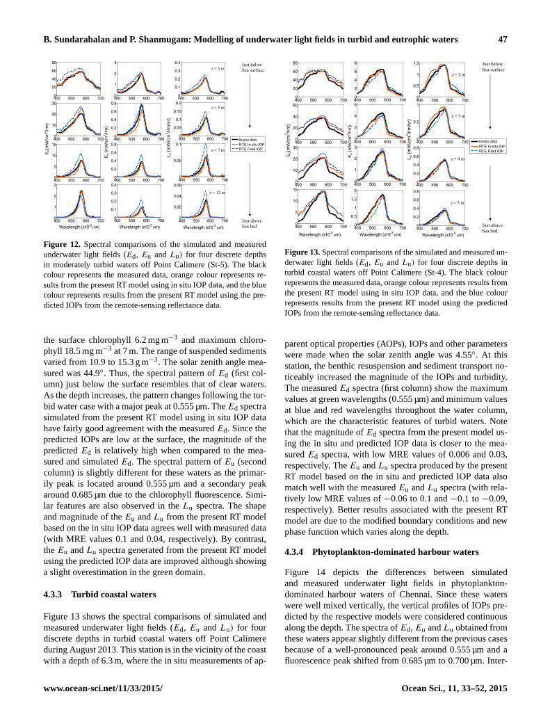
Figure 10. Spectral plots of the in situ IOPs (particulate absorption
ap, particulate attenuation cp, and particulate backscattering bb)
from different waters. (a) Relatively clear waters off Chennai (St-
1), (b) moderately turbid waters off Point Calimere (St-5), (c) turbid
waters off Point Calimere (St-4), (d) phytoplankton-dominated har-
bour waters off Chennai (St-7) and (e) Eutrophic waters off Chennai
(St-8–11).
and predicted IOP profile data are evaluated by compar-
ison with measured underwater radiometric data such as
downwelling irradianceEd(λ, z), upwelling irradianceEu(λ,
z) and upwelling radiance Lu(λ, z). The predicted (from
remote-sensing reflectance data) in situ IOP profile data were
used as inputs for the present RT model. The IOP data mea-
sured from different waters (Fig. 10) include the particulate
absorption (ap), particulate attenuation (cp) and backscatter-
ing (bb).
4.3.1 Clear ocean waters
Figure 11 shows the comparisons of simulated and measured
underwater light fields (Ed, Eu and Lu) for four discrete wa-
ter depths in relatively clear waters off Chennai. Looking
at the Ed spectra (orange colour – present RT model using
in situ IOP data and blue colour – present RT model using
Pred IOP data from remote-sensing reflectance), the max-
imum value is seen at 0.490 µm throughout the water col-
umn. As the depth increases, Ed becomes attenuated in the
blue region (0.400–0.500 µm) but progressively more atten-
uated in the red region (> 0.600 µm). The Ed values from
400 500 600 7000
50
100
150
400 500 600 7000
50
100
400 500 600 7000
50
100
400 500 600 7000
20
40
60
80
400 500 600 7000
2
4
6
400 500 600 7000
2
4
6
400 500 600 7000
1
2
3
4
400 500 600 7000
1
2
3
4
400 500 600 7000
0.5
1
1.5
400 500 600 7000
0.5
1
1.5
400 500 600 7000
0.2
0.4
0.6
0.8
400 500 600 7000
0.2
0.4
0.6
0.8
Eu
(mW
/cm
2 /m
)
L u (
mW
/cm
2 /m
/sr)
Ed(
mW
/cm
2 /m
)
Just below Sea surface
Just above Sea bed
In-situ dataRTE In-situ IOPRTE Pred IOP
z = 2 m
z = 6 m
z = 10 m
z = 14 m
Wavelength (x10-3 m) Wavelength (x10-3 m) Wavelength (x10-3 m)
Figure 11. Spectral comparisons of the simulated and measured
underwater light fields (Ed, Eu and Lu) for four discrete depths
in clear waters off Chennai (St-1). The black colour represents the
measured data, orange colour represents results from the present
RT model using in situ IOP data and the blue colour represents re-
sults from the present RT model using the predicted IOPs from the
remote-sensing reflectance data.
the present RT model using the in situ and predicted IOP
data are closely consistent with measured Ed across the en-
tire visible wavelengths. The simulated Ed yields very low
MRE (at 0.555 µm), 0.03 and −0.01 for the present RT
model using in situ IOP data and predicted IOP data, re-
spectively. Conversely, the spectral pattern of Eu is differ-
ent from that of Ed (second column) displaying two peaks
– one at 0.490 µm (primary) and another at 0.520 µm (sec-
ondary). The Eu from the present RT model using the in situ
IOP data closely matches with measured Eu at most wave-
lengths, except in the region of secondary peak at 0.520 µm.
The MRE (at 0.555 µm) is very low (−0.3) for the present
model using the predicted IOP data. Similar peaks – primary
peak around 0.500 µm and secondary peak around 0.550 µm
– are also seen in the Lu spectrum. As the depth increases
the secondary peak becomes more pronounced due to an in-
crease in turbidity level. The deviation in Lu is very small
for the present RT model as its predicted Lu spectra are well
consistent with the measured Lu spectra, because of the in-
clusion of the effective bottom reflectance instead of the ma-
terial reflectance.
4.3.2 Moderately turbid waters
Figure 12 shows the spectral variations of simulated and
measured underwater light-field data for four discrete depths
in moderately clear waters (with elevated chlorophyll in rela-
tively deep waters as compared to the previous case) off Point
Calimere (August 2012). At this location, the vertical profile
of chlorophyll typically followed the Gaussian pattern, with
Ocean Sci., 11, 33–52, 2015 www.ocean-sci.net/11/33/2015/
B. Sundarabalan and P. Shanmugam: Modelling of underwater light fields in turbid and eutrophic waters 47
400 500 600 7000
0.02
0.04
0.06400 500 600 7000
0.05
0.1400 500 600 7000
0.05
0.1
0.15
0.2400 500 600 7000
0.1
0.2
0.3
0.4
400 500 600 7000
0.1
0.2
0.3
0.4400 500 600 7000
0.2
0.4
0.6
0.8400 500 600 7000
0.2
0.4
0.6
0.8400 500 600 7000
1
2
3
400 500 600 7000
20
40
60
80
400 500 600 7000
10
20
30
400 500 600 7000
5
10
15
400 500 600 7000
1
2
3
Eu
(mW
/cm
2 /m
)
L u (
mW
/cm
2 /m
/sr)
Ed(
mW
/cm
2 /m
)
Just below Sea surface
Just above Sea bed
In-situ dataRTE In-situ IOPRTE Pred IOP
z = 3 m
z = 5 m
z = 7 m
z = 12 m
Wavelength (x10-3 m) Wavelength (x10-3 m) Wavelength (x10-3 m)
Figure 12. Spectral comparisons of the simulated and measured
underwater light fields (Ed, Eu and Lu) for four discrete depths
in moderately turbid waters off Point Calimere (St-5). The black
colour represents the measured data, orange colour represents re-
sults from the present RT model using in situ IOP data, and the blue
colour represents results from the present RT model using the pre-
dicted IOPs from the remote-sensing reflectance data.
the surface chlorophyll 6.2 mg m−3 and maximum chloro-
phyll 18.5 mg m−3 at 7 m. The range of suspended sediments
varied from 10.9 to 15.3 g m−3. The solar zenith angle mea-
sured was 44.9◦. Thus, the spectral pattern of Ed (first col-
umn) just below the surface resembles that of clear waters.
As the depth increases, the pattern changes following the tur-
bid water case with a major peak at 0.555 µm. TheEd spectra
simulated from the present RT model using in situ IOP data
have fairly good agreement with the measured Ed. Since the
predicted IOPs are low at the surface, the magnitude of the
predicted Ed is relatively high when compared to the mea-
sured and simulated Ed. The spectral pattern of Eu (second
column) is slightly different for these waters as the primar-
ily peak is located around 0.555 µm and a secondary peak
around 0.685 µm due to the chlorophyll fluorescence. Simi-
lar features are also observed in the Lu spectra. The shape
and magnitude of the Eu and Lu from the present RT model
based on the in situ IOP data agrees well with measured data
(with MRE values 0.1 and 0.04, respectively). By contrast,
the Eu and Lu spectra generated from the present RT model
using the predicted IOP data are improved although showing
a slight overestimation in the green domain.
4.3.3 Turbid coastal waters
Figure 13 shows the spectral comparisons of simulated and
measured underwater light fields (Ed, Eu and Lu) for four
discrete depths in turbid coastal waters off Point Calimere
during August 2013. This station is in the vicinity of the coast
with a depth of 6.3 m, where the in situ measurements of ap-
400 500 600 7000
5
10
15400 500 600 7000
10
20
30400 500 600 7000
20
40
60400 500 600 7000
20
40
60
80
400 500 600 7000
0.5
1
1.5
2
400 500 600 7000
2
4
6
8
400 500 600 7000
2
4
6
400 500 600 7000
1
2
3
400 500 600 7000
0.2
0.4
0.6
0.8
400 500 600 7000
0.2
0.4
0.6
0.8400 500 600 7000
0.5
1400 500 600 7000
0.5
1
1.5
Eu
(mW
/cm
2 /m
)
L u (
mW
/cm
2 /m
/sr)
Ed(
mW
/cm
2 /m
)
Just below Sea surface
Just above Sea bed
In-situ dataRTE In-situ IOPRTE Pred IOP
z = 2 m
z = 3 m
z = 4 m
z = 5 m
Wavelength (x10-3 m) Wavelength (x10-3 m) Wavelength (x10-3 m)
Figure 13. Spectral comparisons of the simulated and measured un-
derwater light fields (Ed, Eu and Lu) for four discrete depths in
turbid coastal waters off Point Calimere (St-4). The black colour
represents the measured data, orange colour represents results from
the present RT model using in situ IOP data, and the blue colour
represents results from the present RT model using the predicted
IOPs from the remote-sensing reflectance data.
parent optical properties (AOPs), IOPs and other parameters
were made when the solar zenith angle was 4.55◦. At this
station, the benthic resuspension and sediment transport no-
ticeably increased the magnitude of the IOPs and turbidity.
The measured Ed spectra (first column) show the maximum
values at green wavelengths (0.555 µm) and minimum values
at blue and red wavelengths throughout the water column,
which are the characteristic features of turbid waters. Note
that the magnitude of Ed spectra from the present model us-
ing the in situ and predicted IOP data is closer to the mea-
sured Ed spectra, with low MRE values of 0.006 and 0.03,
respectively. The Eu and Lu spectra produced by the present
RT model based on the in situ and predicted IOP data also
match well with the measured Eu and Lu spectra (with rela-
tively low MRE values of −0.06 to 0.1 and −0.1 to −0.09,
respectively). Better results associated with the present RT
model are due to the modified boundary conditions and new
phase function which varies along the depth.
4.3.4 Phytoplankton-dominated harbour waters
Figure 14 depicts the differences between simulated
and measured underwater light fields in phytoplankton-
dominated harbour waters of Chennai. Since these waters
were well mixed vertically, the vertical profiles of IOPs pre-
dicted by the respective models were considered continuous
along the depth. The spectra of Ed, Eu and Lu obtained from
these waters appear slightly different from the previous cases
because of a well-pronounced peak around 0.555 µm and a
fluorescence peak shifted from 0.685 µm to 0.700 µm. Inter-
www.ocean-sci.net/11/33/2015/ Ocean Sci., 11, 33–52, 2015
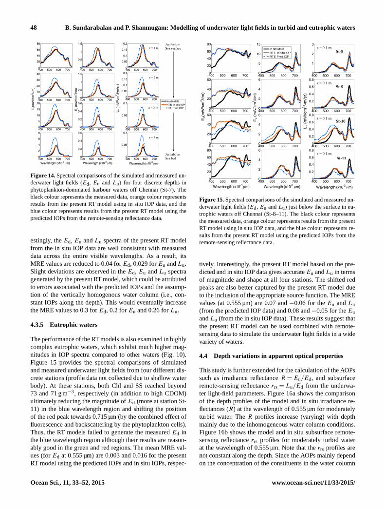
48 B. Sundarabalan and P. Shanmugam: Modelling of underwater light fields in turbid and eutrophic waters
400 500 600 7000
20
40
60
80
400 500 600 7000
10
20
30
40
400 500 600 7000
5
10
15
20
400 500 600 7000
2
4
6
8
400 500 600 7000
0.5
1
1.5
400 500 600 7000
0.5
1
1.5
400 500 600 7000
0.2
0.4
0.6
400 500 600 7000
0.2
0.4
0.6
400 500 600 7000
0.05
0.1400 500 600 7000
0.05
0.1400 500 600 7000
0.05
0.1
0.15
0.2400 500 600 7000
0.05
0.1
0.15
0.2
Eu
(mW
/cm
2 /m
)
L u (
mW
/cm
2 /m
/sr)
Ed(
mW
/cm
2 /m
)
Just below Sea surface
Just above Sea bed
In-situ dataRTE In-situ IOPRTE Pred IOP
z = 1 m
z = 2 m
z = 3 m
z = 4 m
Wavelength (x10-3 m) Wavelength (x10-3 m) Wavelength (x10-3 m)
Figure 14. Spectral comparisons of the simulated and measured un-
derwater light fields (Ed, Eu and Lu) for four discrete depths in
phytoplankton-dominated harbour waters off Chennai (St-7). The
black colour represents the measured data, orange colour represents
results from the present RT model using in situ IOP data, and the
blue colour represents results from the present RT model using the
predicted IOPs from the remote-sensing reflectance data.
estingly, the Ed, Eu and Lu spectra of the present RT model
from the in situ IOP data are well consistent with measured
data across the entire visible wavelengths. As a result, its
MRE values are reduced to 0.04 for Ed, 0.029 for Eu and Lu.
Slight deviations are observed in the Ed, Eu and Lu spectra
generated by the present RT model, which could be attributed
to errors associated with the predicted IOPs and the assump-
tion of the vertically homogenous water column (i.e., con-
stant IOPs along the depth). This would eventually increase
the MRE values to 0.3 for Ed, 0.2 for Eu and 0.26 for Lu.
4.3.5 Eutrophic waters
The performance of the RT models is also examined in highly
complex eutrophic waters, which exhibit much higher mag-
nitudes in IOP spectra compared to other waters (Fig. 10).
Figure 15 provides the spectral comparisons of simulated
and measured underwater light fields from four different dis-
crete stations (profile data not collected due to shallow water
body). At these stations, both Chl and SS reached beyond
73 and 71 g m−3, respectively (in addition to high CDOM)
ultimately reducing the magnitude of Ed (more at station St-
11) in the blue wavelength region and shifting the position
of the red peak towards 0.715 µm (by the combined effect of
fluorescence and backscattering by the phytoplankton cells).
Thus, the RT models failed to generate the measured Ed in
the blue wavelength region although their results are reason-
ably good in the green and red regions. The mean MRE val-
ues (for Ed at 0.555 µm) are 0.003 and 0.016 for the present
RT model using the predicted IOPs and in situ IOPs, respec-
400 500 600 7000
20
40
60
80
400 500 600 7000
20
40
60
400 500 600 7000
20
40
60
400 500 600 7000
20
40
60
80
400 500 600 7000
5
10
15
400 500 600 7000
2
4
6
400 500 600 7000
2
4
6
400 500 600 7000
2
4
6
400 500 600 7000
1
2
3
400 500 600 7000
0.2
0.4
0.6
0.8
400 500 600 7000
0.2
0.4
0.6
0.8
400 500 600 7000
0.2
0.4
0.6
0.8
Eu
(mW
/cm
2 /m
)
L u (
mW
/cm
2 /m
/sr)
Ed(
mW
/cm
2 /m
)
In-situ dataRTE In-situ IOPRTE Pred IOP
St-8
St-9
St-10
St-11
z = 0.1 m
z = 0.1 m
z = 0.1 m
z = 0.1 m
Wavelength (x10-3 m) Wavelength (x10-3 m) Wavelength (x10-3 m)
Figure 15. Spectral comparisons of the simulated and measured un-
derwater light fields (Ed, Eu and Lu) just below the surface in eu-
trophic waters off Chennai (St-8–11). The black colour represents
the measured data, orange colour represents results from the present
RT model using in situ IOP data, and the blue colour represents re-
sults from the present RT model using the predicted IOPs from the
remote-sensing reflectance data.
tively. Interestingly, the present RT model based on the pre-
dicted and in situ IOP data gives accurate Eu and Lu in terms
of magnitude and shape at all four stations. The shifted red
peaks are also better captured by the present RT model due
to the inclusion of the appropriate source function. The MRE
values (at 0.555 µm) are 0.07 and −0.06 for the Eu and Lu
(from the predicted IOP data) and 0.08 and −0.05 for the Eu
and Lu (from the in situ IOP data). These results suggest that
the present RT model can be used combined with remote-
sensing data to simulate the underwater light fields in a wide
variety of waters.
4.4 Depth variations in apparent optical properties
This study is further extended for the calculation of the AOPs
such as irradiance reflectance R = Eu/Ed, and subsurface
remote-sensing reflectance rrs = Lu/Ed from the underwa-
ter light-field parameters. Figure 16a shows the comparison
of the depth profiles of the model and in situ irradiance re-
flectances (R) at the wavelength of 0.555 µm for moderately
turbid water. The R profiles increase (varying) with depth
mainly due to the inhomogeneous water column conditions.
Figure 16b shows the model and in situ subsurface remote-
sensing reflectance rrs profiles for moderately turbid water
at the wavelength of 0.555 µm. Note that the rrs profiles are
not constant along the depth. Since the AOPs mainly depend
on the concentration of the constituents in the water column
Ocean Sci., 11, 33–52, 2015 www.ocean-sci.net/11/33/2015/
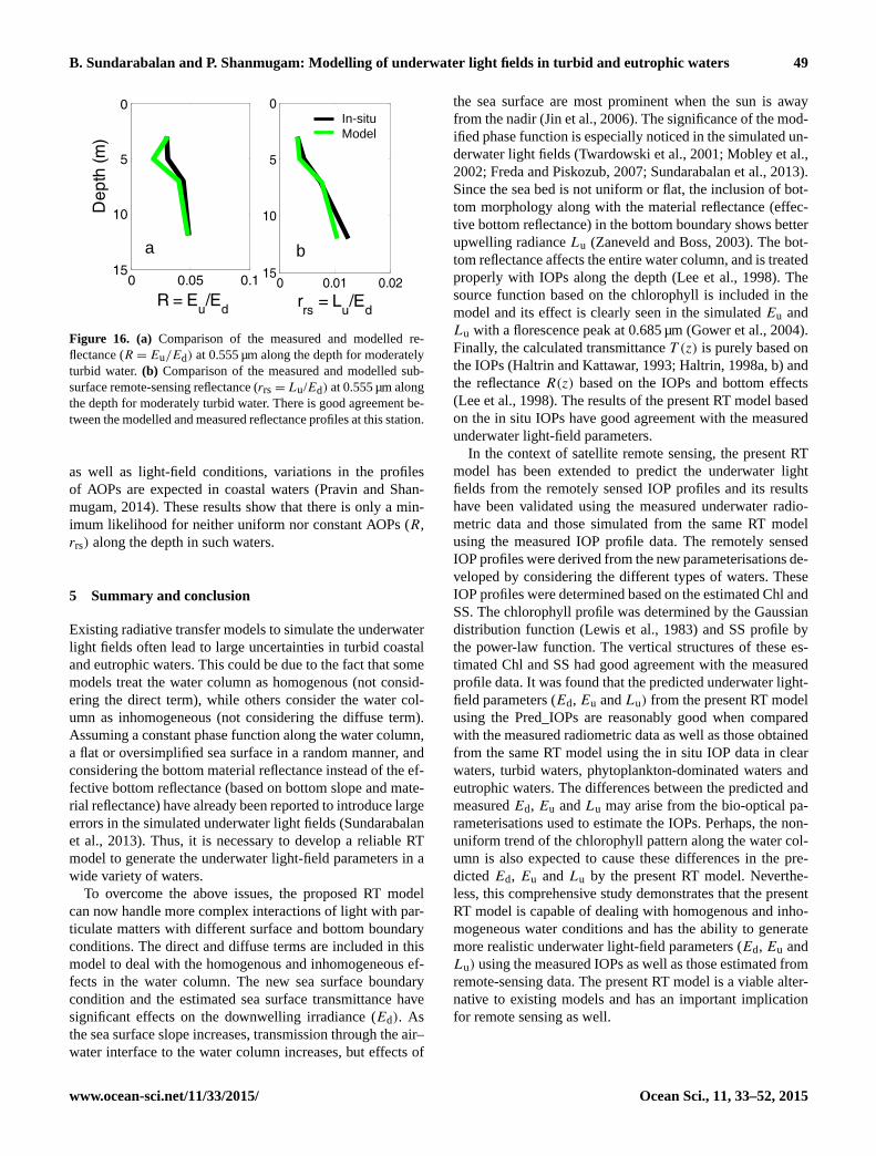
B. Sundarabalan and P. Shanmugam: Modelling of underwater light fields in turbid and eutrophic waters 49
0 0.05 0.1
0
5
10
15
Dep
th (m
)
R = Eu/E
d
0 0.01 0.02
0
5
10
15
rrs
= Lu/E
d
a b
In-situModel
0 0.05 0.1
0
5
10
15
Dep
th (m
)
R = Eu/E
d
0 0.01 0.02
0
5
10
15
rrs
= Lu/E
d
a b
In-situModel
Figure 16. (a) Comparison of the measured and modelled re-
flectance (R = Eu/Ed) at 0.555 µm along the depth for moderately
turbid water. (b) Comparison of the measured and modelled sub-
surface remote-sensing reflectance (rrs = Lu/Ed) at 0.555 µm along
the depth for moderately turbid water. There is good agreement be-
tween the modelled and measured reflectance profiles at this station.
as well as light-field conditions, variations in the profiles
of AOPs are expected in coastal waters (Pravin and Shan-
mugam, 2014). These results show that there is only a min-
imum likelihood for neither uniform nor constant AOPs (R,
rrs) along the depth in such waters.
5 Summary and conclusion
Existing radiative transfer models to simulate the underwater
light fields often lead to large uncertainties in turbid coastal
and eutrophic waters. This could be due to the fact that some
models treat the water column as homogenous (not consid-
ering the direct term), while others consider the water col-
umn as inhomogeneous (not considering the diffuse term).
Assuming a constant phase function along the water column,
a flat or oversimplified sea surface in a random manner, and
considering the bottom material reflectance instead of the ef-
fective bottom reflectance (based on bottom slope and mate-
rial reflectance) have already been reported to introduce large
errors in the simulated underwater light fields (Sundarabalan
et al., 2013). Thus, it is necessary to develop a reliable RT
model to generate the underwater light-field parameters in a
wide variety of waters.
To overcome the above issues, the proposed RT model
can now handle more complex interactions of light with par-
ticulate matters with different surface and bottom boundary
conditions. The direct and diffuse terms are included in this
model to deal with the homogenous and inhomogeneous ef-
fects in the water column. The new sea surface boundary
condition and the estimated sea surface transmittance have
significant effects on the downwelling irradiance (Ed). As
the sea surface slope increases, transmission through the air–
water interface to the water column increases, but effects of
the sea surface are most prominent when the sun is away
from the nadir (Jin et al., 2006). The significance of the mod-
ified phase function is especially noticed in the simulated un-
derwater light fields (Twardowski et al., 2001; Mobley et al.,
2002; Freda and Piskozub, 2007; Sundarabalan et al., 2013).
Since the sea bed is not uniform or flat, the inclusion of bot-
tom morphology along with the material reflectance (effec-
tive bottom reflectance) in the bottom boundary shows better
upwelling radiance Lu (Zaneveld and Boss, 2003). The bot-
tom reflectance affects the entire water column, and is treated
properly with IOPs along the depth (Lee et al., 1998). The
source function based on the chlorophyll is included in the
model and its effect is clearly seen in the simulated Eu and
Lu with a florescence peak at 0.685 µm (Gower et al., 2004).
Finally, the calculated transmittance T (z) is purely based on
the IOPs (Haltrin and Kattawar, 1993; Haltrin, 1998a, b) and
the reflectance R(z) based on the IOPs and bottom effects
(Lee et al., 1998). The results of the present RT model based
on the in situ IOPs have good agreement with the measured
underwater light-field parameters.
In the context of satellite remote sensing, the present RT
model has been extended to predict the underwater light
fields from the remotely sensed IOP profiles and its results
have been validated using the measured underwater radio-
metric data and those simulated from the same RT model
using the measured IOP profile data. The remotely sensed
IOP profiles were derived from the new parameterisations de-
veloped by considering the different types of waters. These
IOP profiles were determined based on the estimated Chl and
SS. The chlorophyll profile was determined by the Gaussian
distribution function (Lewis et al., 1983) and SS profile by
the power-law function. The vertical structures of these es-
timated Chl and SS had good agreement with the measured
profile data. It was found that the predicted underwater light-
field parameters (Ed, Eu and Lu) from the present RT model
using the Pred_IOPs are reasonably good when compared
with the measured radiometric data as well as those obtained
from the same RT model using the in situ IOP data in clear
waters, turbid waters, phytoplankton-dominated waters and
eutrophic waters. The differences between the predicted and
measured Ed, Eu and Lu may arise from the bio-optical pa-
rameterisations used to estimate the IOPs. Perhaps, the non-
uniform trend of the chlorophyll pattern along the water col-
umn is also expected to cause these differences in the pre-
dicted Ed, Eu and Lu by the present RT model. Neverthe-
less, this comprehensive study demonstrates that the present
RT model is capable of dealing with homogenous and inho-
mogeneous water conditions and has the ability to generate
more realistic underwater light-field parameters (Ed, Eu and
Lu) using the measured IOPs as well as those estimated from
remote-sensing data. The present RT model is a viable alter-
native to existing models and has an important implication
for remote sensing as well.
www.ocean-sci.net/11/33/2015/ Ocean Sci., 11, 33–52, 2015
50 B. Sundarabalan and P. Shanmugam: Modelling of underwater light fields in turbid and eutrophic waters
Acknowledgements. This research was supported by INCOIS
under the grant (OEC1314117INCOPSHA) of the SATCORE
program. We thank D. Rajasekhar, The Head, Vessel Management
Cell (VMC), and the Director of National Institute of Ocean
Technology (NIOT) for providing Coastal Research Vessels to
Indian Institute of Technology (IIT) Madras, Chennai, India for
conducting various bio-optical measurements in coastal waters off
Point Calimere and Chennai on the southeast coast of India. We are
thankful to the scientists N. Ravi and K. Shashikumar of VMC for
arranging the vessels to make the necessary measurements. We are
thankful to the anonymous reviewers for their valuable comments
to improve the quality of this manuscript.
Edited by: O. Zielinski
References
Ahn, Y. H.: Optical properties of biogenous and mineral particles
present in the ocean. Application: inversion of reflectance, PhD
Thesis, Paris-VI University, 1990.
Ahn, Y. H. and Shanmugam, P.: Detecting red tides from Satellite
Ocean color observations in optically complex Northeast-Asia
coastal waters, Remote Sens. Environ., 103, 419–437, 2006.
Antoine, D., André, J. M., and Morel, A.: Oceanic primary pro-
duction: 2.Estimation at global scale from satellite (coastal zone
colour scanner) chlorophyll, Global Biogeochem. Cy., 10, 57–
69, 1996.
Arrigo, K. R., Matrai, P. A., and van Dijken, G. L.: Primary produc-
tivity in the Arctic Ocean: Impacts of complex optical properties
and subsurface chlorophyll maxima on large-scale estimates, J.
Geophys. Res., 116, C11022, doi:10.1029/2011JC007273, 2011.
Babin, M., Stramski, D., Ferrari, G. M., Claustre, H., Bricaud, A.,
Obolensky, G., and Hoepffner, N.: Variations in the light absorp-
tion coefficients of phytoplankton, nonalgal particles, and dis-
solved organic matter in coastal waters around Europe, J. Geo-
phys. Res., 108, C73211, doi:10.1029/2001JC000882, 2003.
Bricaud, A., Babin, M., Morel, A., and Claustre, H.: Variability in
the chlorophyll-specific absorption coefficients of natural phyto-
plankton: analysis and parameterization, J. Geophys. Res., 100,
13321–13332, 1995.
Cherkasheva, A., Nöthig, E.-M., Bauerfeind, E., Melsheimer, C.,
and Bracher, A.: From the chlorophyll a in the surface layer to
its vertical profile: a Greenland Sea relationship for satellite ap-
plications, Ocean Sci., 9, 431–445, doi:10.5194/os-9-431-2013,
2013.
Dmitriev, E. V., Khomenko, G., Chami, M., Sokolov, A. A.,
Churilova, T. Y., and Korotaev, G. K.: Parameterization of light
absorption by components of seawater in optically complex
coastal waters of the Crimea Peninsula (Black Sea), Appl. Opt.,
48, 1249–1261, 2009.
Freda, W. and Piskozub, J.: Improved method of Fournier–Forand
marine phase function parameterization, Opt. Exp., 20, 12763–8,
2007.
Gjerstad, K. I., Stamnes, J. J., Hamre, B., Lotsberg, J. K., Yan, B.,
and Stamnes, K.: Monte Carlo and Discrete-Ordinate Simula-
tions of Irradiances in the Coupled Atmosphere-Ocean System,
Appl. Opt., 42, 2609–2621, 2003.
Gokul, R. E., Shanmugam, P., and Sundarabalan, V. B.: Inversion
models for deriving inherent optical properties and their vertical
profiles in coastal waters, Cont. Shelf Res., 84, 120–138, 2014.
Gordon, H. R. and Morel, A.: Remote assessment of ocean colour
for interpretation of satellite visible imagery: A review, Lecture
notes on coastal and estuarine studies, Springer Verlag Heidel-
berg, Germany, 1983.
Gordon, H. R., Brown, O. B., and Jacobs, M. M.: Computed rela-
tionships between the inherent and apparent optical properties of
a flat homogeneous ocean, Appl. Opt., 14, 417–427, 1975.
Gower, J. F. R., Brown, L., and Borstad, G. A.: Observation of
chlorophyll fluorescence in west coast waters of Canada using
the MODIS satellite sensor, Can. J. Remote Sens., 30, 17–25,
2004.
Haltrin, V. I.: Self-consistent approach to the solution of the light
transfer problem for irradiances in marine waters with arbitrary
turbidity, depth, and surface illumination. I. Case of absorption
and elastic scattering, Appl. Opt., 37, 3773–3784, 1998a.
Haltrin, V. I.: Apparent optical properties of the sea illuminated by
Sun and sky: case of the optically deep sea, Appl. Opt., 37, 8336–
8340, 1998b.
Haltrin, V. I.: One-parameter two-term Henyey–Greenstein phase
function for light scattering in seawater, Opt. Exp., 41, 1022–8,
2002.
Haltrin, V. I.: About nonlinear dependence of Remote Sensing and
Diffuse reflection coefficients on Gordon’s Parameter, Proceed-
ings of the II International Conference “Current Problems in Op-
tics of Natural Waters,” ONW’2003, edited by: Levin, I. and
Gilbert, G., St. Petersburg, Russia, 363–369, 2003.
Haltrin, V. I. and Kattawar, G. W.: Self-consistent solutions to
the equation of transfer with elastic and inelastic scattering in
oceanic optics, I. Model, Appl. Opt., 32, 5356–5367, 1993.
Hoepffner, N. and Sathyendranath, S.: Bio-optical Characteristics of
coastal waters: Absorption spectra of phytoplankton and pigment
distribution in the western North Atlantic, Limnol. Oceanogr.,
37, 1660–1679, 1992.
Hollstein, A. and Fischer, J.: Radiative transfer solutions for cou-
pled atmosphere ocean systems using the matrix operator tech-
nique, J. Quant. Spectrosc. Radiat. Transfer., 113, 536–548,
2012.
Huot, Y., Morel, A., Twardowski, M. S., Stramski, D., and
Reynolds, R. A.: Particle optical backscattering along a chloro-
phyll gradient in the upper layer of the eastern South Pa-
cific Ocean, Biogeosciences, 5, 495–507, doi:10.5194/bg-5-495-
2008, 2008.
Jin, Z., Charlock, T. P., Rutledge, K., Stamnes, K., and Wang,
Y.: Analytical solution of radiative transfer in the coupled
atmosphere–ocean system with a rough surface, Appl. Opt., 45,
7443–7455, 2006.
Kirk, J. T. O.: Monte Carlo study of the nature of the underwater
light field in, and the relationships between optical properties of,
turbid yellow waters, Aust. J. Mar. Freshwater Res., 32, 517–532,
1981.
Lee, W. L. and Liou, K. N.: A coupled atmosphere–ocean radiative
transfer system using the analytic Four-Stream approximation, J.
Atmos. Sci., 64, 3681–3694, 2007.
Lee, Z. P., Carder, K. L., Mobley, C. D., Steward, R. G., and Patch,
J. S.: Hyperspectral remote sensing for shallow waters. I. A semi-
analytical model, Appl. Opt., 37, 6329–6338, 1998.
Ocean Sci., 11, 33–52, 2015 www.ocean-sci.net/11/33/2015/
B. Sundarabalan and P. Shanmugam: Modelling of underwater light fields in turbid and eutrophic waters 51
Lee, Z. P., Carder, K. L., Mobley, C. D., Steward, R. G., and Patch, J.
S.: Hyperspectral remote sensing for shallow waters: 2. Deriving
bottom depths and water properties by optimization, Appl. Opt.,
38, 3831–3843, 1999.
Lewis, M. R., Cullen, J. J., and Platt, T.: Phytoplankton and thermal
structure in the upper ocean: Consequences of non-uniformity in
chlorophyll profile, J. Geophys. Res., 88, 2565–2570, 1983.
Martin, J., Tremblay, J. E., Gagnon, J., Tremblay, G., Lapoussiere,
A., Jose, C., Poulin, M., Gosselin, M., Gratton, Y., and Michel,
C.: Prevalence, structure and properties of subsurface chlorophyll
maxima in Canadian Arctic waters, Mar. Ecol.-Prog. Ser., 412,
69–84, 2010.
Matsuoka, A., Hill, V., Huot, Y., Babin, M., and Bricaud, A.: Sea-
sonal variability in the light absorption properties of western Arc-
tic waters: Parameterization of the individual components of ab-
sorption for ocean colour applications, J. Geophys. Res., 116,
C02007, doi:10.1029/2009JC005594, 2011.
Mobley, C. D.: Light and water: radiative transfer in natural waters,
San Diego: Academic Press, Inc., 1994.
Mobley, C. D., Sundman, L. K., and Boss, E.: Phase function effects
on oceanic light fields, Appl. Opt., 41, 1035–50, 2002.
Morel, A.: Optical modelling of the upper ocean in relation to its
biogenous matter content (Case 1 waters), J. Geophys. Res., 93,
10749–10768, 1988.
Morel, A.: Light and marine photosynthesis: a spectral model with
geochemical and climatological implications, Prog. Oceanogr.,
26, 263–306, 1991.
Morel, A. and Berthon, J. R.: Surface pigments, algal biomass pro-
files, and potential production of the euphotic layer: Relation-
ships reinvestigated in view of remote-sensing application, Lim-
nol. Oceanogr., 34, 1545–1562, 1989.
O’Reilly, J. E., Maritorena, S., Mitchell, B. G., Siegel, D. A.,
Carder, K. L., Garver, S. A., Kahru, M., and McClain, C.: Ocean
colour algorithms for SeaWiFS, J. Geophys. Res., 103, 24937–
24953, 1998.
O’Reilly, J. E., Maritorena, S., O’Brien, M. C., Siegel, D. A., Toole,
D., Menzies, D., Smith, R. C., Mueller, J. L., Mitchell, B. G.,
Kahru, M., Chavez, F. P., Strutton, P., Cota, G. F., Hooker, S. B.,
McClain, C. R., Carder, K. L., Karger, F. M., Harding, L., Mag-
nuson, A., Phinney, D., Moore, G. F., Aiken, J., Arrigo, K. R.,
Letelier, R., and Culver, M.: Ocean Colour Chlorophyll a Algo-
rithms for SeaWiFS, OC2 and OC4: Version 4, NASA Technical
Memorandum, 11, 9–23, 2000.
Pierson, W. J. and Moskowitz, L.: Proposed spectral form for fully
developed wind seas based on similarity theory of S. A. Kitaig-
orodskii, J. Geophys. Res., 69, 5181–5190, 1964.
Pegau, W. S., Gray, D., and Zaneveld, J. R. V.: Absorption and at-
tenuation of visible and near-infrared light in water: dependence
on temperature and salinity, Appl. Opt., 36, 6035–6046, 1997.
Platt, T. and Sathyendranath, S.: Oceanic Primary Production: Es-
timation by Remote Sensing at Local and Regional Scales, Sci-
ence, 241, 1613–1620, 1988.
Pope, R. M. and Fry, E. S.: Absorption spectrum (380–700 nm) of
pure water. II. Integrating cavity measurements, Appl. Opt., 36,
8710–8723, 1997.
Pravin, J. D. and Shanmugam, P.: A new model for the subsurface
irradiance reflectance in clear and turbid waters, Opt. Exp., 22,
9548–9566, 2014.
Prieur, L. and Sathyendranath, S.: An optical classification of
coastal and oceanic waters based on the specific spectral absorp-
tion curves of phytoplankton pigments, dissolved organic matter,
and other particulate materials, Limnol. Oceanogr., 26, 671–689,
1981.
Ramakrishnan, R., Rajawat, A. S., and Chauhan, O. S.: Suspended
sediment concentration profiles from synoptic satellite observa-
tions, IEEE J. Sel. Topics Appl. Earth Observ. Remote Sens., 6,
2051–2057, 2013.
Sathyendranath, S. and Platt, T.: Remote sensing of ocean chloro-
phyll: consequence of non-uniform pigment profile, Appl. Opt.,
28, 490–495, 1988.
Shanmugam, P.: A new bio-optical algorithm for the remote sensing
of algal blooms in complex ocean waters, J. Geophys. Res., 116,
C04016, doi:10.1029/2010JC006796, 2011a.
Shanmugam, P.: New models for retrieving and partitioning
coloured dissolved organic matter in the global oceans. Impli-
cations for remote sensing, Remote Sens. Environ., 115, 1501–
1521, 2011b.
Shanmugam, P., Ahn, Y. H., Ryu, J. H., and Sundarabalan, V. B.:
An evaluation of inversion models for retrieval of inherent opti-
cal properties from ocean colour in coastal and open sea waters
around Korea, J. Oceanogr., 66, 815–830, 2010.
Shanmugam, P., Sundarabalan, V. B., Ahn, Y. H., and Ryu, J. H. A.:
New Inversion Model to Retrieve the Particulate Backscattering
in Coastal/Ocean Waters, IEEE Trans. Geosci. Remote Sens., 49,
2463–74, 2011.
Smith, R. C.: Ocean colour for the estimation of Global marine pri-
mary productivity, Workshop on the Global Ocean Flux study,
Woods Hole, Masschusetts, 103–110, 1984.
Smith, R. C. and Baker, K. S.: Optical properties of the clearest
natural waters (200–800 nm), Appl. Opt., 20, 177–184, 1981.
Stamnes, K., Tsay, S., Wiscombe, W., and Jayaweera, K.: Nu-
merically stable algorithm for discrete-ordinate-method radiative
transfer in multiple scattering and emitting layered media, Appl.
Opt., 27, 2502–2509, 1988.
Stramska, M. and Stramski, D.: Effects of a non-uniform verti-
cal profile of chlorophyll concentration on remote-sensing re-
flectance of the ocean, Appl. Opt., 44, 1735–1747, 2005.
Stramski, D., Bricaud, A., and Morel, A.: Modelling the inherent
optical properties of the ocean based on the detailed composition
of the planktonic community, Appl. Opt., 40, 2929–2945, 2001.
Sundarabalan, V. B., Shanmugam, P., and Manjusha, S. S.: Radia-
tive transfer modelling of upwelling lightfield in coastal waters,
J. Quant. Spectrosc. Radiat. Transfer., 121, 30–44, 2013.
Twardowski, M. S., Boss, E., Macdonald, J. B., Pegau, W. S.,
Barnard, A. H., and Zaneveld, J. R. V.: A model for estimating
bulk refractive index from the optical backscattering ratio and the
implications for understanding particle composition in case I and
case II waters, J. Geophys. Res., 106, 14129–14142, 2001.
Uitz, J., Claustre, H., Morel, A., and Hooker, S. B.: Vertical dis-
tribution of phytoplankton communities in open ocean: An as-
sessment based on surface chlorophyll, J. Geophys. Res., 111,
C08006, doi:10.1029/2005JC003207, 2006.
Wang, Y., Liu, D., Song, K., Du, J., Wang, Z., Zhang, B., Tang,
X., Lei, X., and Wu, Y.: Characterization of Water Constituents
Spectra Absorption in Chagan Lake of Jilin Province, Northeast
China, Chin. Geogra. Sci., 21, 34–345, 2011.
www.ocean-sci.net/11/33/2015/ Ocean Sci., 11, 33–52, 2015

52 B. Sundarabalan and P. Shanmugam: Modelling of underwater light fields in turbid and eutrophic waters
Wozniak, S. B. and Stramski, D.: Modelling the optical properties
of mineral particles suspended in seawater and their influence on
ocean reflectance and chlorophyll estimation from remote sens-
ing algorithms, Appl. Opt., 43, 3489–3503, 2004.
Zaneveld, J. R. V. and Boss, E.: The influence of bottom morphol-
ogy on reflectance: theory and two-dimensional geometry model,
Limnol. Oceanogr., 48, 374–379, 2003.
Zhang, Y., Liu, M., Qin, B., Woerd, H. J., Li, J., and Li, Y.: Mod-
elling remote-sensing reflectance and retrieving Chlorophyll-a
concentration in extremely turbid case-2 waters (lake Taihu,
China), IEEE Trans. Geosci. Remote Sens., 47, 1937–1948,
2009.
Ocean Sci., 11, 33–52, 2015 www.ocean-sci.net/11/33/2015/