Nonnegative matrix factorization with the Itakura-Saito divergence. With application

to music analysis

Factorisation en matrices à coefficients positifs avec la divergence d’Itakura-Saito. Application à

l’analyse de la musique

Cédric Févotte Nancy Bertin

Jean-Louis Durrieu

Mai 2005

Mai 2008

Département Traitement du signal et des Images Groupe AAO : Audio, Acoustique et Ondes

2008D006

Nonnegative matrix factorization with theItakura-Saito divergence. With application to

music analysis.

Factorisation en matrices a coefficients positifs avec ladivergence d’Itakura-Saito. Application a l’analyse de la

musique.

Cedric Fevotte, Nancy Bertin and Jean-Louis Durrieu

LTCI (CNRS & TELECOM ParisTech)37-39, rue Dareau, 75014 Paris, France.

1

AbstractThis article presents theoretical, algorithmic and experimental results about nonnegative ma-trix factorization (NMF) with the Itakura-Saito (IS) divergence. We describe how IS-NMFis underlain by a well-defined statistical model of superimposed Gaussian components andis equivalent to maximum likelihood estimation of variance parameters. This setting can ac-commodate regularization constraints on the factors through Bayesian priors. In particular,inverse-Gamma and Gamma Markov chain priors are considered in this work. Estimationcan be carried out using a space-alternating generalized expectation-maximization (SAGE)algorithm; this leads to a novel type of NMF algorithm, whose convergence to a stationarypoint of the IS cost function is guaranteed.We also discuss the links between the IS divergence and other cost functions used in NMF,in particular the Euclidean distance and the generalized Kullback-Leibler (KL) divergence.As such, we describe how IS-NMF can also be performed using a gradient multiplicative al-gorithm (a standard algorithm structure in NMF) whose convergence is observed in practice,though not proven.Finally, we report a furnished experimental comparative study of Euclidean-NMF, KL-NMF and IS-NMF algorithms applied to the power spectrogram of a short piano sequencerecorded in real conditions, with various initializations and model orders. Then we showhow IS-NMF can successfully be employed for denoising and upmix (mono to stereoconversion) of an original piece of early jazz music. These experiments indicate thatIS-NMF correctly captures the semantics of audio and is better suited to the representationof music signals than NMF with the usual Euclidean and KL costs.

Keywords: Nonnegative matrix factorization (NMF), unsupervised machine learning,Bayesian linear regression, space-alternating generalized expectation-maximization (SAGE),music transcription, single-channel source separation, audio restoration, computational au-ditory scene analysis (CASA).

ResumeCet article presente des resultats theoriques, algorithmiques et experimentaux concernantla factorisation en matrices a coefficients positifs (NMF) avec la divergence d’Itakura-Saito (IS). Nous decrivons comment la IS-NMF peut etre interpretee comme un problemed’estimation au sens du maximum de vraisemblance de parametres de variance dans unmodele de composantes gaussiennes. Cette interpretation statistique permet notammentde prendre en compte des contraintes de regularisation des facteurs, dans un formalismebayesien. L’estimation des parametres peut etre conduite en utilisant un algorithme de typeSAGE, donnant lieu a un nouveau type d’algorithme NMF dont la convergence vers un pointstationnaire du critere est garantie.Dans cet article, nous evoquons egalement les liens entre la divergence IS et d’autres fonctionscouts utilisees en NMF, notamment la distance euclidienne et la divergence de Kullback-Leibler (KL) generalisee. Ainsi, nous montrons comment la IS-NMF peut egalement etrerealisee par le biais d’un algorithme multiplicatif (une methode courante en NMF), dont laconvergence n’est cependant pas montree, bien que constatee en pratique.Finalement, nous rapportons les resultats d’une etude experimentale dans laquelle nousavons compare les factorisations obtenues de plusieurs algorithmes NMF, avec les coutseuclidiens, KL et IS, appliques au spectrogramme d’un court extrait de piano. Puis, nousdecrivons comment la IS-NMF peut etre utilisee dans contexte de restauration audio, pourle debruitage et le remixage mono vers stereo d’un enregistrement de jazz ancien. Lesresultats indiquent que IS-NMF extrait correctement la semantique des donnees, et estmieux adaptee a la representation du signal musical que la NMF avec les couts euclidiensou KL.

Mots-cles: Factorisation en matrices a coefficients positifs, apprentissage statistiquenon-supervise, regression lineaire bayesienne, algorithme SAGE, transcription musicale,separation de sources avec un seul capteur, restauration audio, analyse de scenes auditives.

2

1 Introduction

Nonnegative matrix factorization (NMF) is a now popular dimension reduction technique, em-ployed for non-subtractive, part-based representation of nonnegative data. Given a data matrix Vof dimensions F ×N with nonnegative entries, NMF is the problem of finding a factorization

V ≈WH (1)

where W and H are nonnegative matrices of dimensions F × K and K × N , respectively. K isusually chosen such that F K +KN << F N , hence reducing the data dimension. Note that thefactorization is in general only approximate, so that the terms “approximate nonnegative matrixfactorization” or “nonnegative matrix approximation” also appear in the literature. NMF has beenused for various problems in diverse fields. To cite a few, let us mention the problems of learningparts of faces and semantic features of text (Lee and Seung, 1999), polyphonic music transcription(Smaragdis and Brown, 2003), object characterization by reflectance spectra analysis (Berry et al.,2007), portfolio diversification (Drakakis et al., 2007), as well as Scotch whiskies clustering (Younget al., 2006).

In the literature, the factorization (1) is usually sought after through the minimization problem

minW,H≥0

D(V|WH) (2)

where D(V|WH) is a cost function defined by

D(V|WH) =F∑f=1

N∑n=1

d([V]fn|[WH]fn) (3)

and where d(x|y) is a scalar cost function. Popular choices are the Euclidean distance, that wehere define as

dEUC(x|y) =12

(x− y)2 (4)

and the (generalized) Kullback-Leibler (KL) divergence, also referred to as I-divergence, definedby

dKL(x|y) = x logx

y− x+ y . (5)

Both cost functions are positive, and take value zero if and only if x = y.Lee and Seung (2001) proposed gradient descent algorithms to solve the minimization prob-

lem (2) under the latter two cost functions. Using a suitable step size, the gradient descentupdate rules are turned into multiplicative rules, under which the cost function is shown to benon-increasing. The simplicity of the update rules has undoubtedly contributed to the popularityof NMF, and most of the above-mentioned applications are based on Lee and Seung’s algorithmfor minimization of either the Euclidean distance or the KL divergence.

Nevertheless, some papers have considered NMF under other cost functions. As such, Kompass(2007) considers a parametric generalized divergence which interpolates between the Euclidean dis-tance and the KL divergence, with a single parameter. As a matter of fact, the divergence coincidesup to a factor with the β-divergence introduced by Eguchi and Kano (2001). The β-divergence isalso considered by Cichocki et al. (2006), as is the family of Csiszar divergences (to which Amari’sα-divergence belongs). Finally, Dhillon and Sra (2005) describe algorithms for the wide familyof Bregman divergences. Again these papers come up with multiplicative gradient descent NMFalgorithms, the convergence of which being proved only in certain cases, as discussed later.

In this paper we are interested in NMF with the Itakura-Saito (IS) divergence, whose expressionis given by

dIS(x|y) =x

y− log

x

y− 1 . (6)

This divergence was obtained by Itakura and Saito (1968) from the maximum likelihood (ML)estimation of short-time speech spectra under autoregressive modeling. It was presented as “a

3

measure of the goodness of fit between two spectra” and became popular in the speech commu-nity during the seventies. It was in particular praised for the good perceptual properties of thereconstructed signals it led to (Gray et al., 1980).

As we shall see, this divergence has other interesting properties. It is in particular scale-invariant, meaning that low energy components of V bear the same relative importance as highenergy ones. This is relevant to situations in which the coefficients of V have a large dynamicrange, such as in audio short-term spectra. The IS divergence also leads to desirable statisticalinterpretations of the NMF problem. Indeed, we describe how NMF can in this case be recast asmaximum likelihood (ML) estimation of W and H in superimposed signals under simple Gaussianassumptions. Equivalently, we describe how IS-NMF can be interpreted as ML of W and H inmultiplicative Gamma noise.

The IS divergence belongs to the class of Bregman divergences and is a limit case of the β-divergence. Thus, the gradient descent multiplicative rules given in (Dhillon and Sra, 2005) and(Cichocki et al., 2006) – which coincide in the IS case – can be applied. If convergence of thisalgorithm is observed in practice, its proof is still an open problem. The statistical frameworkgoing along with IS-NMF allows to derive a new type of minimization method, derived from space-alternating expectation-maximization (SAGE), a variant of the standard expectation-maximization(EM) algorithm. This method leads to new update rules, which do not possess a multiplicativestructure. The EM setting guarantees convergence of this algorithm to a stationary point of thecost function. Moreover, the statistical framework opens doors to Bayesian approaches for NMF,allowing elaborate priors on W and H, for which maximum a posteriori (MAP) estimation canagain be performed using SAGE. Examples of such priors, yielding regularized estimates of W andH, are presented in this work.

IS-NMF underlies previous works in the area of automatic music transcription and single-channel audio source separation, but never explicitly so. In particular our work builds on (Benaroyaet al., 2003, 2006; Abdallah and Plumbley, 2004; Plumbley et al., 2006) and the connections be-tween IS-NMF and these papers will be discussed.

This article is organized as follows. Section 2 addresses general properties of IS-NMF. Therelation between the IS divergence and other cost functions used in NMF is discussed in Section 2.1,Section 2.2 addresses scale invariance and Section 2.3 describes the statistical interpretations of IS-NMF. Section 3 presents two IS-NMF algorithms; an existing multiplicative algorithm is describedin Section 3.1 while Section 3.2 introduces a new algorithm derived from SAGE. Section 4 reportsan experimental comparative study of Euclidean-NMF, KL-NMF or IS-NMF algorithms appliedto the power spectrogram of a short piano sequence recorded in real conditions, with variousinitializations and model orders. These experiments show that IS-NMF correctly captures thesemantics of the signal and is better suited to the representation of audio than NMF with theusual Euclidean and KL costs. Section 5 presents how IS-NMF can accommodate regularizationconstraints on W and H within a Bayesian framework and how SAGE can be adapted to MAPestimation. In particular, we give update rules for IS-NMF with Gamma and inverse-GammaMarkov chain priors on the rows of H. In Section 6, we present audio restoration results of anoriginal early recording of jazz music; we show how the proposed regularized IS-NMF algorithmscan successfully be employed for denoising and upmix (mono to stereo conversion) of the originaldata. Finally, conclusions and perspectives of this work are given in Section 7.

2 Properties of NMF with the Itakura-Saito divergence

In this section we address the links between the IS divergence and other cost functions used forNMF, then we discuss its scale invariance property and finally describe the statistical interpreta-tions of IS-NMF.

4

2.1 Relation to other divergences used in NMF

β-divergence The IS divergence is a limit case of the β-divergence introduced by Eguchi andKano (2001), that we here define as

dβ(x|y) def=

1

β (β−1)

(xβ + (β − 1) yβ − β x yβ−1

)β ∈ R\{0, 1}

x (log x− log y) + (y − x) β = 1xy − log x

y − 1 β = 0(7)

Eguchi and Kano (2001) assume β > 1, but the definition domain can very well be extended toβ ∈ R, as we do. The β-divergence is easily shown to be continuous in β by using the identitylimα→0 x

α/α = log x. It coincides up to a factor 1/β with the generalized divergence of Kompass(2007) which, in the context of NMF, was constructed as to interpolate between the KL divergence(β = 1) and the Euclidean distance (β = 2). Note that the derivative of dβ(x|y) with respect to(wrt) y is also continuous in β, and simply writes

∇y dβ(x|y) = yβ−2 (y − x). (8)

The derivative shows that dβ(x|y), as a function of y, has a single minimum in y = x and that itincreases with |y−x|, justifying its relevance as a measure of fit. Figure 1 represents the Euclidean,KL and IS divergences for x = 1.

Using equation (8), the gradients of criterion Dβ(V|WH) wrt W and H simply writes

∇HDβ(V|WH) = WT((WH).β−2. (WH−V)

)(9)

∇WDβ(V|WH) =((WH).β−2. (WH−V)

)HT (10)

where . denotes Hadamard entrywise product and A.n denotes the matrix with entries [A]nij . Themultiplicative gradient descent approach taken in (Lee and Seung, 2001; Cichocki et al., 2006;Kompass, 2007) is equivalent to updating each parameter by multiplying its value at previousiteration by the ratio of the negative and positive parts of the derivative of the criterion wrtthis parameter, namely θ ← θ.[∇f(θ)]−/[∇f(θ)]+, where ∇f(θ) = [∇f(θ)]+ − [∇f(θ)]− and thesummands are both nonnegative. This ensures nonnegativity of the parameter updates, providedinitialization with a nonnegative value. A fixed point θ? of the algorithm implies either ∇f(θ?) = 0or θ? =0. This leads to the following updates,

H ← H.WT ((WH).β−2.V)

WT (WH).β−1(11)

W ← W.((WH).β−2.V) HT

(WH).β−1 HT(12)

where AB denotes the matrix A.B.−1. Lee and Seung (1999) showed that Dβ(V|W H) is non-

increasing under the latter updates for β = 2 (Euclidean distance) and β = 1 (KL divergence).Kompass (2007) generalizes the proof to the case 1 ≤ β ≤ 2. In practice, we observe that thecriterion is still nonincreasing under updates (11) and (12) for β < 1 and β > 2 (and in particularfor β = 0, corresponding to the IS divergence), but no proof is available. Indeed, the proof given byKompass makes use of the convexity of dβ(x|y) as a function of y, which is only true for 1 ≤ β ≤ 2.In the rest of the paper, the term “EUC-NMF” will be used as a shorthand for “Euclidean-NMF”.

Bregman divergences The IS divergence belongs to the class of Bregman divergences, definedas dφ(x|y) = φ(x) − φ(y) − ∇φ(y) (x − y), where φ is a strictly convex function of R that has acontinuous derivative ∇φ. The IS divergence is obtained with φ(y) = − log(y). Using the sameapproach as in previous paragraph, Dhillon and Sra (2005) derive the following update rules forminimization of Dφ(V|WH),

H ← H.WT (∇2φ(WH).V)

WT (∇2φ(WH).WH)(13)

W ← W.(∇2φ(WH).V) HT

(∇2φ(WH).WH) HT(14)

5

Again, the authors observed in practice continual descent of Dφ(V|WH) under these rules, butwere not able to give a proof of convergence. Note that equations (11) and (12) coincide withequations (13) and (14) for the IS divergence.

2.2 Scale invariance

The following property holds for any value of β,

dβ(γ x|γ y) = γβ dβ(x|y). (15)

It implies that the IS divergence is scale-invariant (i.e, dIS(γ x|γ y) = dIS(x|y)), and is the onlyone of the β-divergence family to possess this property. The scale invariance means that samerelative weight is given to small and large coefficients of V in cost function (3), in the sense thata bad fit of the factorization for a low-power coefficient [V]fn will cost as much as a bad fit forhigher power coefficient [V]f ′n′ . On the opposite, factorizations obtained with β > 0 (such as withthe Euclidean distance or the KL divergence) will rely more heavily on the largest coefficients andless precision is to be expected in the estimation of the low-power components.

The scale invariance of the IS divergence is relevant to decomposition of audio spectra, whichtypically exhibit exponential power decrease along frequency f and also usually comprise low-powertransient components such as note attacks together with higher power components such as tonalparts of sustained notes. The results of the decomposition of a piano spectrogram presented inSection 4 confirm these expectations by showing that IS-NMF extracts components correspondingto very low residual noise and hammer hits on the strings with great accuracy. These componentsare either ignored or severely degraded when using Euclidean or KL divergences.

2.3 Statistical interpretations

We now turn to statistical interpretations of IS-NMF which will eventually lead to a new EM-basedalgorithm, described in Section 3.

2.3.1 Notations

The entries of matrices V, W and H are denoted vfn, wfk and hkn respectively. Lower casebold letters will in general denote columns, such that W = [w1, . . . ,wK ], while lower case plainletters with a single index denote rows, such that H = [hT1 , . . . , h

TK ]T . We also define the matrix

V = WH, whose entries are denoted vfn. Finally, we introduce the matrices W−k and H−k whichrespectively denote matrix W of which column k has been removed and matrice H of which rowk has been removed. Where these conventions clash, the intended meaning should be clear fromthe context.

2.3.2 Sum of Gaussians

Theorem 1 (IS-NMF as ML estimation in sum of Gaussians). Consider the generative model definedby, ∀n = 1, . . . , N

xn =K∑k=1

ck,n (16)

where xn and ck,n belong to CF×1 and

ck,n ∼ Nc(0, hkn diag (wk)), (17)

where Nc(µ,Σ) denotes the proper multivariate complex Gaussian distribution and where thecomponents c1,n, . . . , cK,n are mutually independent and individually independently distributed.Define V as the matrix with entries vfn = |xfn|2. Then, maximum likelihood estimation of Wand H from X = [x1, . . . ,xN ] is equivalent to NMF of V into V ≈WH, where the Itakura-Saitodivergence is used.

6

Proof. Under assumptions of Theorem 1 and using the expression ofNc(µ,Σ) given in Appendix A,

the minus log likelihood function CML,1(W,H) def= − log p(X|W,H) simply factorizes as

CML,1(W,H) = −N∑n=1

F∑f=1

logNc

(xfn|0,

∑k

wfk hkn

)(18)

= NF log π +N∑n=1

F∑f=1

log

(∑k

wfk hkn

)+

|xfn|2

(∑k wfk hkn)

(19)

c=N∑n=1

F∑f=1

dIS

(|xfn|2 |

∑k

wfk hkn

)(20)

where c= denotes equality up to constant terms. The minimization of CML,1(W,H) wrt W andH thus amounts to the NMF V ≈WH with the IS divergence. Note that Theorem 1 holds alsofor real-valued Gaussian components. In that case CML,1(W,H) equals DIS(V|WH) up to aconstant and a factor 1/2.

The generative model (16) was introduced by Benaroya et al. (2003, 2006) for single-channelaudio source separation. In that context, xn = [x1n, . . . , xfn, . . . , xFn]T is the Short-Time FourierTransform (STFT) of an audio signal x, where n = 1, . . . , N is a frame index and f = 1, . . . , F is afrequency index. The signal x is assumed to be the sum of two sources x = s1 + s2 and the STFTsof the sources are modeled as s1,n =

∑K1k=1 ck,n and s2,n =

∑K1+K2k=K1+1 ck,n, with K1 +K2 = K. This

means that each source STFT is modeled as a sum of elementary components each characterized bya Power Spectral Density (PSD) wk modulated in time by frame-dependent activation coefficientshkn. The PSDs characterizing each source are learnt on training data, before the mixture spec-trogram |X|.2 is decomposed onto the known dictionary W = [w1, . . . ,wK1 ,wK1+1, . . . ,wK1+K2 ].However, in these papers, the PSDs and the activation coefficients are estimated separately usingsomewhat ad-hoc strategies (the PSDs are learnt with vector quantization) and the equivalencebetween ML estimation and IS-NMF is not fully exploited.

The generative model (16) may be viewed as a generalization of well-known models of com-posite signals. For example, inference in superimposed components with Gaussian structure canbe tracked back to (Feder and Weinstein, 1988). In that paper however, the components are as-sumed stationary and solely modeled by their PSD wk, which is in turn parametrized by a setof parameters of interest θk, to be estimated. One extension brought in equation (16) is the ad-dition of the amplitude parameters H. This however has the inconvenient of making the totalnumber of parameters F K + KN dependent of N , with the consequence of losing asymptoticaloptimality properties of ML estimation. But note that it is precisely the addition of the amplitudeparameters in the model that allows W to be treated as a set of possibly identifiable parame-ters. Indeed, if hkn is set to 1 for all k and n the variance of xn becomes

∑k wk for all n, i.e,

is equal to the sum of the parameters. This obviously makes each PSD wk not uniquely identifiable.

Very interestingly, the equivalence between IS-NMF and ML inference in sum of Gaussian com-ponents provides means of reconstructing the components ck,n with a sense of statistical optimality,which contrasts with NMF using other divergences where methods of reconstructing componentsfrom the factorization WH are somewhat ad-hoc (see below). Indeed, given W and H, minimummean square error (MMSE) estimates can be obtained through Wiener filtering, such that

ck,fn =wfk hkn∑Kl=1 wfl hln

xfn. (21)

The Wiener gains summing up to 1 for a fixed entry (f, n) the decomposition is conservative, i.e,

xn =K∑k=1

ck,n. (22)

7

Note that a consequence of Wiener reconstruction is that the phase of all components ck,fn is equalto the phase of xfn.

Most works in audio have considered the NMF of magnitude spectra |X| instead of power spectra|X|.2, see, e.g, (Smaragdis and Brown, 2003; Smaragdis, 2007; Virtanen, 2007; Bertin et al., 2007).In that case, it can be noted (see, e.g, Virtanen et al. (2008)), that KL-NMF is related to the MLproblem of estimating W and H in the model structure

|xn| =K∑k=1

|ck,n| (23)

under Poissonian assumptions, i.e, ck,fn ∼ P(wfkhkn), where P(λ) is the Poisson distribution,defined in Appendix A. Indeed, the sum of Poisson random variables being Poissonian itself (withthe shape parameters summing up as well), one obtains xfn ∼ P(

∑Kk=1 wfkhkn). Then, it can

easily be seen that the likelihood − log p(X|W,H) is equal up to a constant to DKL( |X| |W H).Here, W is homogeneous to a magnitude spectrum and not to a power spectrum. After factor-ization, component estimates are typically formed using the phase of the observations (Virtanen,2007), such that

ck,fn = wfk hkn arg(xfn), (24)

where arg(x) denotes the phase of complex scalar x. This approach is worth a few comments.First, the Poisson distribution is formerly only defined for integers, which impairs statistical inter-pretation of KL-NMF on non-countable data such as audio spectra. Second, this approach enforcesnonnegativity somehow arbitrarily way by taking the absolute value of data X. In contrast, withthe Gaussian modelling, nonnegativity arises naturally through the variance fitting problem equiv-alence. Similarly, the reconstruction method enforces the components to have same phase asobservation coefficients, while this is only a consequence of Wiener filtering in the Gaussian mod-elling framework. Last, the component reconstruction method is not statistically-grounded and isnot conservative, i.e xn ≈

∑Kk=1 ck,n. Note that Wiener reconstruction is used with KL-NMF of

the magnitude spectrum |X| by Smaragdis (2007), where it is presented as spectral filtering andits conservativity is pointed out.

2.3.3 Multiplicative noise

Theorem 2 (IS-NMF as ML estimation in Gamma multiplicative noise). Consider the generativemodel

V = (WH) .E (25)

where E is multiplicative independent and identically-distributed (i.i.d.) Gamma noise with mean1. Then, maximum likelihood estimation of W and H is equivalent to NMF of V into V ≈WH,where the Itakura-Saito divergence is used.

Proof. Let us note {efn} the entries of E. We have vfn = vfn efn, with p(efn) = G(efn|α, β), andwhere G(x|α, β) is the Gamma probability density function (pdf) defined in Appendix A. Under

the i.i.d. noise assumption, the minus log likelihood CML,2(W,H) def= − log p(V|W,H) writes

CML,2(W,H) = −∑f,n

log p(vfn|vfn) (26)

= −∑f,n

log G (vfn/vfn|α, β) /vfn (27)

c= β∑f,n

vfnvfn− α

βlog

vfnvfn− 1 (28)

The ratio α/β is simply the mean of the Gamma distribution. When it is equal to 1, we obtainthat CML,2(θ) is equal to DIS(V|V) = DIS(V|W H) up to a positive factor and a constant.

8

Algorithm 1 IS-NMF/MUInput : nonnegative matrix VOutput : nonnegative matrices W and H such that V ≈WHInitialize W and H with nonnegative valuesfor i = 1 : niter do

H← H.WT ((WH).−2.V)WT (WH).−1

W←W. ((WH).−2.V) HT

(WH).−1 HT

Normalize W and Hend for

The multiplicative noise equivalence explains the scale invariance of the IS divergence, becausethe noise acts as a scale factor on vfn. On the opposite, EUC-NMF is equivalent to ML likelihoodestimation of W and H in additive i.i.d. Gaussian noise. The influence of additive noise is greateron coefficients of V with small amplitude (i.e, low SNR) than on the largest ones. As to KL-NMF, it neither corresponds to multiplicative nor additive noise but actually corresponds to MLestimation in Poisson noise.1 To summarize, we have

EUC-NMF: p(vfn|vfn) = N (vfn|vfn, σ2), (29)KL-NMF: p(vfn|vfn) = P(vfn|vfn), (30)

IS-NMF: p(vfn|vfn) =1vfnG(vfnvfn|α, 1

α

), (31)

and in all cases, E{vfn|vfn} = vfn.

Theorem 2 reports in essence how Abdallah and Plumbley (2004) derive a “statistically mo-tivated error measure”, which happens to be the IS divergence, in the very similar context ofnonnegative sparse coding (see also developments in Plumbley et al. (2006)). Pointing out thescale invariance of this measure, this work leads Virtanen (2007) to consider the IS divergence(but again without referring to it as such) for NMF in the context of single-channel source sepa-ration, but the algorithm is applied to the magnitude spectra instead of the power spectra, losingstatistical coherence, and the sources are reconstructed through equation (24) instead of Wienerfiltering.

3 Algorithms for NMF with the Itakura-Saito divergence

In this section we describe two algorithms for IS-NMF. The first one has a multiplicative structureand is only a special case of the derivations of Section 2.1. The second one is of a novel type,EM-based, and is derived from the statistical presentation of IS-NMF as given in Theorem 1.

3.1 Multiplicative gradient descent algorithm

A multiplicative gradient descent IS-NMF algorithm is obtained by either setting β = 0 in (11)and (12) or setting φ(y) = − log(y) in (13) and (14). The resulting update rules coincide and leadto Algorithm 1. These update rules were also obtained by Abdallah and Plumbley (2004), priorto (Dhillon and Sra, 2005; Cichocki et al., 2006). In the following, we refer to this algorithm as“IS-NMF/MU”. This algorithm includes a normalization step at every iteration, which eliminatestrivial scale indeterminacies leaving the cost function unchanged. We impose ‖wk‖2 = 1 and scalehk accordingly. Again, we emphasize that continual descent of the cost function is observed inpractice with this algorithm, but that we were not able to come up with a proof of convergence.

1KL-NMF is wrongly presented as ML in additive Poisson noise in numerous publications.

9

3.2 SAGE algorithm

We now describe an EM-based algorithm for estimation of the parameters θ = {W,H}, derivedfrom the statistical formalism introduced in Theorem 1. The additive structure of the generativemodel (16) allows to update the parameters describing each component Ck

def= [ck,1, . . . , ck,N ]separately, using SAGE (Fessler and Hero, 1994). SAGE is an extension of EM for data modelswith particular structures, including data generated by superimposed components. It is knownto converge faster in iterations than standard EM, though one iteration of SAGE is usually morecomputationally demanding than EM as it usually requires to update the sufficient statistics “moreoften”. Let us consider a partition of the parameter space θ =

⋃Kk=1 θk with

θk = {wk, hk} , (32)

where we recall that wk is the kth column of W and hk is the kth row of H. The SAGE algorithminvolves choosing for each subset of parameters θk a hidden-data space which is complete for thisparticular subset. Here, the hidden-data space for θk is simply chosen to be Ck

def= [ck,1, . . . , ck,N ].An EM-like functional is then built for each subset θk as the conditional expectation of the minuslog likelihood of Ck, which writes

QMLk (θk|θ′)

def= −∫Ck

log p(Ck|θk) p(Ck|X,θ′) dCk. (33)

One iteration i of the SAGE algorithm then consists of computing (E-step) and minimizing (M-step) QML

k (θk|θ′) for k = 1, . . . ,K. Note that θ′ always contains the most up-to-date parametersvalue, and not only the values at iteration i − 1 like in standard EM. This leads to the above-mentioned increase in computational burden, which is mild in our case.

The derivations of the SAGE algorithm for IS-NMF are detailed in Appendix B. However, for afixed k, the E-step merely consists of computing the posterior power Vk of component Ck, definedby [Vk]fn = vk,fn = |µpostk,fn|2 + λpostk,fn, where µpostk,fn and λpostk,fn are the posterior mean and varianceof ck,fn, given by

µpostk,fn =wfk hkn∑l wfl hln

xfn, (34)

λpostk,fn =wfk hkn∑l wfl hln

∑l 6=k

wfl hln. (35)

The M-step is then shown to amount to the following one-component NMF problem

minwk, hk≥0

DIS(V′k |wk hk) (36)

where V′k denotes Vk as computed from θ′. Interestingly, in the one-component case, the gradientssimplify to

∇hkn QMLk (wk, hk|θ′) =

F

hkn− 1h2kn

F∑f=1

v′k,fnwfk

, (37)

∇wfk QMLk (wk, hk|θ′) =

N

wfk− 1w2fk

N∑n=1

v′k,fnhkn

. (38)

The gradients are easily zeroed, leading to the following updates

h(i+1)kn =

1F

∑f

v′k,fn

w(i)fk

, (39)

w(i+1)fk =

1N

∑n

v′k,fn

h(i+1)kn

, (40)

10

Algorithm 2 IS-NMF/EMInput : nonnegative matrix VOutput : nonnegative matrices W and H such that V ≈WHInitialize W and H with nonnegative valuesfor i = 1 : niter do

for k = 1 : K doCompute Gk = wkhk

WH % Wiener gainCompute Vk = Gk.(Gk.V + W−kH−k) % Posterior power of Ck

hk ← 1F (w.−1

k )T Vk % Update row k of Hwk ← 1

NVk (h.−1k )T % Update column k of W

Normalize wk and hkend for

end for

% Note that WH = V needs to be computed only once, at initialization.Indeed, W−kH−k can be computed as V − wold

k holdk before V is subsequently

updated as V = W−kH−k + wnewk hnewk .

which guarantees QMLk (w(i+1)

k , h(i+1)k |θ′) ≤ QML

k (w(i)k , h

(i)k |θ

′). This can also be written in matrixform, as shown in Algorithm 2, which summarizes the SAGE algorithm for IS-NMF. In the follow-ing, we will refer to this algorithm as “IS-NMF/EM”.

IS-NMF/EM and IS-NMF/MU have same complexity O(12FKN) per iteration, but can leadto different run times, as shown in the results below. Indeed, in our Matlab implementation,the operations in IS-NMF/MU can be efficiently vectorized using matrix entrywise multiplication,while IS-NMF/EM requires looping over the components, which is more time consuming.

The convergence of IS-NMF/EM to a stationary point of DIS(V|WH) is granted by propertyof SAGE. However, it can only converge to a point in the interior domain of the parameter space,i.e, W and H cannot take entries equal to zero. This is seen in equation (36): if either wfk orhkn is zero, then the cost dIS(v′k,fn|wfkhkn) becomes infinite. This is not a feature shared byIS-NMF/MU, which does not a priori exclude zero coefficients in W and H (but excludes vfn = 0,which would lead to a division by zero). However, because zero coefficients are invariant undermultiplicative updates (see Section 2.1), if IS-NMF/MU attains a fixed point solution with zeroentries, then it cannot be determined if the limit point is a stationary point. Yet, if the limitpoint does not take zero entries (i.e, belongs to the interior of the parameter space) then it is astationary point, which may or may not be a local minimum. This is stressed by Berry et al. (2007)for EUC-NMF but holds for IS-NMF/MU as well.

Note that SAGE has been used in the context of single-channel source separation by Ozerovet al. (2007) for inference on a model somehow related to the IS-NMF model (16). Indeed, theseauthors address voice/music separation using a generative model of the form xn = cV,n + cM,n

where the first component represents voice while the second one represents music. Then, eachcomponent is given a Gaussian mixture model (GMM). The GMM parameters for voice are learntfrom training data, while the music parameters are adapted to data. Though related, the GMMand NMF models are quite different in essence. The first one expresses the signal as a sum of twocomponents that can each take different states. The second one expresses the signal as a sum ofK components, each representative of one object. It cannot be claimed that one model is betterthan the other, but that they rather address different characteristics. It is anticipated that thetwo models can be used jointly within the SAGE framework, for example, by modelling voice cV,nwith a GMM (i.e, a specific component with many states) and music cM,n with a NMF model (i.e,a composite signal with many components).

11

4 Analysis of a short piano excerpt

In this section we report an experimental comparative study of the above-mentioned NMF al-gorithms applied to the spectrogram of a short monophonic piano sequence. In a first step wecompare the results of multiplicative Euclidean, KL and IS NMF algorithms for several values ofK, before we more specifically compare the multiplicative and EM-based algorithms for IS-NMFin a second step.

4.1 Experimental setup

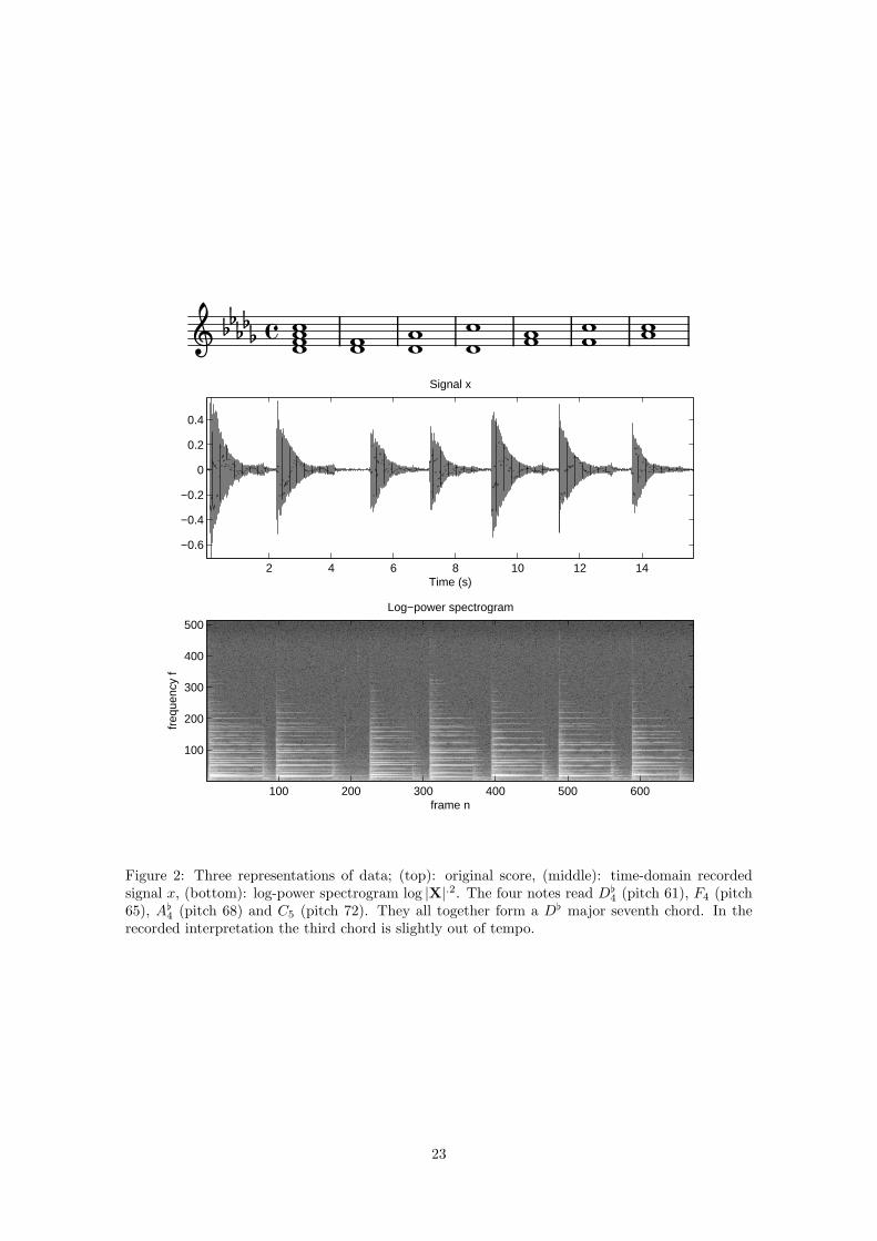
A real piano sequence, played from score given in figure 2 on a Yamaha DisKlavier MX100A up-right piano, was recorded in a small size room by a Schoeps omnidirectional microphone, placedabout 15 cm (6 in) above the opened body of the piano. The sequence is composed of 4 notes,played all at once in the first measure and then played by pairs in all possible combinations in thesubsequent measures. The 15.6 seconds long recorded signal was downsampled to νs = 22050 Hz,yielding T = 339501 samples. A STFT X of x was computed using a sinebell analysis window oflength L = 1024 (46 ms) with 50 % overlap between two frames, leading to N = 674 frames andF = 513 frequency bins. The time-domain signal x and its log-power spectrogram are representedon figure 2.

IS-NMF/MU, IS-NMF/EM and the multiplicative gradient descent NMF algorithms with Eu-clidean and KL costs were implemented in Matlab and run on data V = |X|.2. Note that in thefollowing the terms “EUC-NMF” and “KL-NMF” will implicitly refer to the multiplicative imple-mentation of these NMF techniques. All algorithms were run for several values of the number ofcomponents, more specifically for K = 1, . . . , 10. For each value of K, 10 runs of each algorithmwere produced from 10 random initializations of W and H, chosen, in Matlab notations, as W =abs(randn(F,K)) + ones(F,K) and H = abs(randn(K,N)) + ones(K,N). The algorithms wererun for niter = 5000 iterations.

4.2 Pitch estimation

In the following results, it will be observed that some of the basis elements (columns of W) have apitched structure, characteristic of individual musical notes. If pitch estimation is not the objectiveper se of the following study, it is informative to check if correct pitch values can be inferred fromthe factorization. As such, a fundamental frequency (or pitch) estimator is applied using themethod described in (Vincent et al., 2007). It consists in computing dot products of wk with a setof J frequency combs and retaining the pitch number corresponding to the largest dot product.Each comb is a cosine function with period fj , scaled and shifted to the amplitude interval [0 1],that takes its maximum value 1 at bins multiple of fj . The set of fundamental frequency binsfj = νj

νsL is indexed on the MIDI logarithmic scale, i.e, such that

νj = 440× 2pj−69

12 . (41)

The piano note range usually goes from pmin = 21, i.e, note A0 with fundamental frequencyfmin = 27.5 Hz, to pmax = 108, i.e, note C8 with frequency fmax = 4186 Hz. Two adjacent keysare separated by a semitone (∆p = 1). The MIDI pitch number of the notes pictured on figure 2are 61 (D[

4), 65 (F4), 68 (A[4) and 72 (C5), and were chosen arbitrarily. In our implementation ofthe pitch estimator, the MIDI range was sampled from 20.6 to 108.4 with step 0.2. In the following,an arbitrary pitch value of 0 will be given to unpitched basis elements; the classification of pitchedand unpitched elements was done manually by looking at the basis elements and listening to thecomponent reconstructions.

4.3 Results and discussion

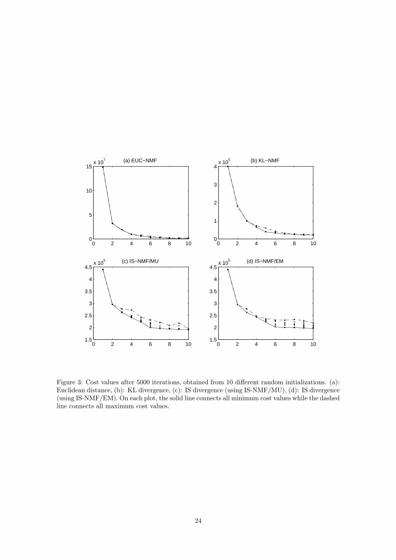
Convergence behavior and algorithm complexities Run times of 1000 iterations of each ofthe four algorithms are shown in Table 1, together with the algorithm complexities. Figure 3 showsfor each algorithm and for every value of K the final cost values of the 10 runs, after the 5000

12

algorithm iterations. A first observation is that the minimum and maximum cost values differs, forK > 4 in the Euclidean case, K > 3 in the KL case and K > 2 in the IS case. This either meansthat the algorithms have failed to converge after 5000 iterations in some cases, or suggests thepresence of local minima. Figure 4 displays for all 4 algorithms the evolution of the cost functionsalong the 5000 iterations for all of the 10 runs, in the particular case K = 6.

Evolution of the factorizations with order K In this paragraph we examine in details theunderlying semantics of the factorizations obtained with all three cost functions. We here onlyaddress the comparison of factorizations obtained from the three multiplicative algorithms. IS-NMF/EM and IS-NMF/MU will be more specifically compared in the next paragraph. Otherwisestated, the factorizations studied below are those obtained from the run yielding the minimumcost value among the 10 runs. Figures 5 to 8 display the columns of W and corresponding rowsof H. The columns of W are represented against frequency bin f on the left (in log10 amplitudescale) while the rows of H are represented against frame index n on the right (in linear amplitudescale). Pitched components are displayed first (top to down, in ascending order of estimated pitchvalue), followed by the unpitched components. For sake of conciseness only part of the results arereproduced in this article but we emphasize that the factorizations obtained with all four algorithmsfor K = 4, 5, 6 are available online at (Companion Web Site), together with sound reconstructionsof the individual components. Component STFTs Ck were computed by applying the Wienerfilter (21) to X using the factors W and H obtained with all 3 cost functions. Time-domaincomponents ck were then reconstructed by inverting the STFTs using an adequate overlap-addprocedure with dual synthesis window. By conservativity of Wiener reconstruction and linearityof the inverse-STFT, the time-domain decomposition is also conservative, i.e, such that

x =K∑k=1

ck. (42)

Common sense suggests that choosing as many components as notes forms a sensible guess forthe value of K, so as to obtain a meaningful factorization of |X|.2 where each component would beexpected to represent one and only one note. The factorizations obtained with all three costs forK = 4 prove that this is not the case. Euclidean and KL-NMF rather successfully extracts notes65 and 68 into separate components (second and third), but notes 61 and 72 are melted into thefirst component while a fourth component seems to capture transient events corresponding to thenote attacks (sound of the hammer hitting the string) and the sound produced by the release of thesustain pedal. The first two components obtained with IS-NMF have a similar interpretation tothose given by EUC-NMF and KL-NMF. However the two other components differ in nature: thethird component comprise note 68 and transients, while the fourth component is akin to residualnoise. It is interesting to notice how this last component, though of much lower energy than theothers components (in the order of 1 compared to 104 for the others) bears equal importance inthe decomposition. This is undoubtedly a consequence of the scale invariance property of the ISdivergence discussed in Section 2.2.

A fully separated factorization (at least as intended) is obtained for K = 5 with KL-NMF, asdisplayed on figure 5. This results in four components each made up of a single note and a fifthcomponent containing sound events corresponding to note attacks and pedal releases. Howeverthese latter events are not well localized in time, and suffer from an unnatural tremolo effect (oscil-lating variations in amplitudes), as can be heard from the reconstructed sound files. Surprisingly,the decomposition obtained with EUC-NMF by setting K = 5, results in splitting the second com-ponent of the K = 4 decomposition in two components with estimated pitches 65 and 65.4, insteadof actually demixing the third component which comprised notes 61 and 72. As for IS-NMF, thefirst component now groups notes 61 and 68, the second and third components respectively capturenotes 65 and 72, the fourth component is still akin to residual noise, while the fifth componentperfectly renders the attacks and releases.

Full separation of the individual notes is finally obtained with Euclidean and IS costs for K = 6,as shown on figures 6 and 7. KL-NMF produces an extra component (with pitch estimate 81) which

13

is not clearly interpretable, and is in particular not akin to residual noise as could have been hopedfor. The decomposition obtained with the IS cost describes as follows. The four first componentscorrespond to individual notes whose pitch estimate match exactly the pitches of the notes played.The visual aspect of the PSDs is much better than the basis elements learnt from EUC-NMF andKL-NMF. The fifth component captures the hammer hits and pedal releases with great accuracyand the sixth component is akin to residual noise.

When the decomposition is carried on beyond K = 6, it is observed that EUC-NMF andKL-NMF split existing components into several subcomponents (such as components capturingsustained and decaying parts of one note) with pitch in the neighborhood of the note fundamentalfrequency. On the opposite, IS-NMF/MU spends the extra components in fine-tuning the rep-resentation of the low energy components, i.e, residual noise and transient events (as such, thehammer hits and pedal releases eventually get split in two distincts components). As such, forK = 10, the pitch estimates reads EUC-NMF: [61 64.8 64.8 65 65 65.8 68 68.4 72.2 0], KL-NMF:[61 61 65 65 66 68 72 80.2 0 0], IS-NMF/MU: [61 61 65 68 72 0 0 0 0 0]. If note 61 is indeed splitin 2 components with IS-NMF/MU, one of the two components is actually inaudible.

The message we want to bring out from this experimental study is the following. The natureof the decomposition obtained with IS-NMF, and its progression as K increases, is in accord withan object-based representation of music, close to our own comprehension of sound. Entities withwell-defined semantics emerge from the decomposition (individual notes, hammer hits, pedal re-leases, residual noise) while the decompositions obtained from the Euclidean and KL costs are lessinterpretable from this perspective. We need to mention that these conclusions do not always holdwhen the factorization is not the one yielding the lowest cost values from the 10 runs. As such,we also examined the factorizations with highest cost values (with all three cost functions) andwe found out that they did not reveal the same semantics, which was in turn not always easilyinterpretable. The upside however is that lowest IS cost values correspond to the most desirablefactorizations indeed, so that IS-NMF “makes sense”.

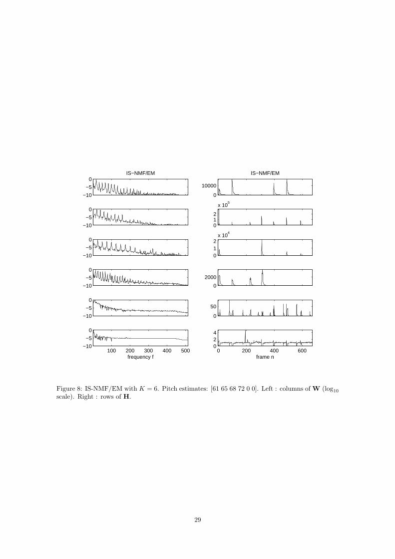
Comparison of multiplicative and EM-based IS-NMF Algorithms IS-NMF/MU and IS-NMF/EM are designed to address the same task of minimizing the cost DIS(V|WH), so that theachieved factorization should be identical in nature provided they complete this task. As such,the progression of the factorization provided by IS-NMF/EM is similar to the one observed forIS-NMF/MU and described in the previous paragraph. However, the resulting factorizations arenot exactly equivalent, because IS-NMF/EM does not inherently allow zeros in the factors (seeSection 3.2). This feature can be desirable for W as the presence of sharp notches in the spectrummay not be physically realistic for audio, but can be considered a drawback as far as H is concerned.Indeed, the rows of H being akin to activation coefficients, when a sound object k is not presentin frame n, then hkn should be strictly zero. These remarks probably explain the factorizationobtained from IS-NMF/EM with K = 6, displayed on figure 8. The notches present in the PSDslearnt with IS-NMF/MU, as seen on figure 7, have disappeared from the PSDs on figure 8, whichexhibit better regularity. Unfortunately, IS-NMF/EM does not fully separate out the note attacksin the fifth component, like IS-NMF/MU does. Indeed, parts of the attacks appear in the secondcomponent, and the rest appears in the fifth component, which also contains the pedal releases.This is possibly explained by the a priori high sparsity of a transients component, which can behandled by IS-NMF/MU but not IS-NMF/EM (because it does not allow zero values in H). Notethat increasing the number of components K or the number of algorithm iterations niter does notsolve this specific issue.

Regarding compared convergence of the algorithms, IS-NMF/MU decreases the cost functionmuch faster in the initial iterations and, with this data set, attains lower final cost values thanIS-NMF/EM, as shown on figure 3 or figure 4 for K = 6. As already mentioned, though the twoalgorithms have the same complexity, the run time per iteration of IS-NMF/MU is smaller thanIS-NMF/EM for K > 3, see Table 1.

14

5 Regularized IS-NMF

We now describe how the statistical setting going along with IS-NMF can be exploited to incor-porate regularization constraints/prior information in the factors estimates.

5.1 Bayesian setting

We consider a Bayesian setting where W and H are given (independent) prior distributions p(W)and p(H). We are looking for a joint MAP estimate of W and H through minimization of criterion

CMAP (W,H) def= − log p(W,H|X) (43)c= DIS(V|WH)− log p(W)− log p(H) (44)

When independent priors of the form p(W) =∏k p(wk) and p(H) =

∏k p(hk) are used, then the

SAGE algorithm presented in Section 3.2 can again be used for MAP estimation. In that case, thefunctionals to be minimized for each component k write

QMAPk (θk|θ′)

def= −∫Ck

log p(θk|Ck) p(Ck|X,θ′) dCk (45)

c= QMLk (wk, hk|θ′)− log p(wk)− log p(hk) (46)

Thus, the E-step still amounts to computing QMLk (wk, hk|θ′), as done in Section 3.2, and only the

M-step is changed by the regularization constraints − log p(wk) and − log p(hk) which now needto be taken into account.

Next we more specifically consider Markov chain priors favoring smoothness over the rows ofH. In the following results no prior structure will be assumed for W (i.e, W is estimated throughML). However, we stress that the methodology presented for the rows of H can equivalently betransposed to the columns of W, that prior structures can be imposed on both W and H andthat these structures need not to belong to the same class of models. Note also that since thecomponents are treated separately, they can each be given a different type of model (for examplesome components could be assigned a GMM, as discussed at the end of Section 3.2).

We assume the following prior structure for hk,

p(hk) =N∏n=2

p(hkn|hk(n−1)) p(hk1), (47)

where p(hkn|hk(n−1)) is a pdf with mode hk(n−1). The motivation behind this prior is to constrainhkn not to differ significantly from its value at entry n − 1, hence favoring smoothness of theestimate. Possible pdf choices are, for n = 2, . . . , N ,

p(hkn|hk(n−1)) = IG(hkn|α, (α+ 1)hk(n−1)) (48)

andp(hkn|hk(n−1)) = G(hkn|α, (α− 1)/hk(n−1)) (49)

where G(x|α, β) is the previously introduced Gamma pdf, with mode (α − 1)/β (for α ≥ 1) andIG(x|α, β) is the inverse-Gamma pdf (see Appendix A), with mode β/(α + 1). Both priors areconstructed so that their mode is obtained for hkn = hk(n−1). α is a shape parameter that controlsthe sharpness of the prior around its mode. A high value of α will increase sharpness and willthus accentuate smoothness of hk while a low value of α will render the prior more diffuse andthus less constraining. The two priors become actually very similar for large values of α, as shownon figure 9. In the following, hk1 is assigned the scale-invariant Jeffreys noninformative priorp(hk1) ∝ 1/hk1.

15

5.2 New updates

Under prior structure (47), the derivative of QMAPk (wk, hk|θ′) wrt hkn writes, ∀n = 2, . . . , N − 1,

∇hkn QMAPk (wk, hk|θ′) =

∇hkn QMLk (wk, hk|θ′)−∇hkn log p(hk(n+1)|hkn)−∇hkn log p(hkn|hk(n−1)) (50)

This is shown to be equal to

∇hkn QMAPk (wk, hk|θ′) =

1h2kn

(p2 h2kn + p1 hkn + p0) (51)

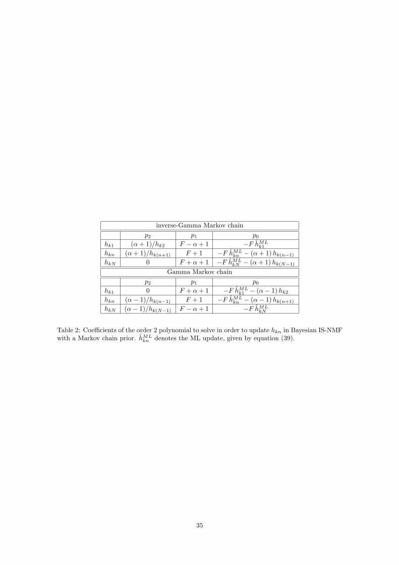
where the values of p0, p1 and p2 are specific to the type of prior employed (Gamma or inverse-Gamma chains), as given in Table 2. Updating hkn then simply amounts to solving an order 2polynomial. The polynomial has only one nonnegative root, given by

hkn =

√p2

1 − 4 p2 p0 − p1

2 p2. (52)

The coefficients hk1 and hkN at the borders of the Markov chain require specific updates, but theyalso only require solving polynomials of order either 2 or 1, with coefficients given in Table 2 as well.

Note that the difference between the updates with the Gamma and inverse-Gamma chains priormainly amounts to interchanging the positions of hk(n−1) and hk(n+1) in p0 and p2. Interestingly,it can be noticed that using a backward Gamma chain prior p(hk) =

∏N−1n=1 p(hkn|hk(n+1)) p(hkN )

with shape parameter α is actually equivalent (in terms of MAP updates) to using a forwardinverse-Gamma chain prior as in equation (47) with shape parameter α− 2. Respectively, using abackward inverse-Gamma chain prior with with shape parameter α is equivalent to using a “for-ward” Gamma chain prior with with shape parameter α+ 2.

Note that Virtanen et al. (2008) have recently considered Gamma chains for regularization ofKL-NMF. The modelling proposed in their work is however different than ours. Their Gammachain prior is constructed in a hierarchical setting, i.e, by introducing extra auxiliary variables, soas to ensure conjugacy of the priors with the Poisson observation model. Estimation of the factorsis then carried out with the standard gradient descent multiplicative approach and single-channelsource separation results are presented from the factorization of the magnitude spectrogram |X|with component reconstruction (24).

6 Learning the semantics of music with IS-NMF

The aim of the experimental study proposed in Section 4 was to analyze the results of several NMFalgorithms on a short, simple and well-defined musical sequence, with respect to the cost function,initialization and model order. We now present results of NMF on a long polyphonic recording.Our goal is to examine how much of the semantics can NMF learn from the signal, with a fixednumber of components and a fixed random initialization. This is not easily assessed numericallyin the most general context, but quantitative evaluations could be performed on specific tasks insimulation settings. Such tasks could include music transcription, like in (Abdallah and Plumbley,2004), single-channel source separation, like in Benaroya et al. (2003, 2006) or content-based musicretrieval based on NMF features.

Rather than choosing and addressing one of these specific tasks, we here propose to use NMFin a real-case audio restoration scenario, where the purpose is to denoise and upmix originalmonophonic material (one channel) to stereo (two channels). This task is very close to single-channel source separation, with the difference that we are here not aiming at perfectly separatingeach of the sources, but rather isolating subsets of coherent components that can be given differentdirections of arrival in the stereo remaster so as to render a sensation of spatial diversity. Wewill show in particular that the addition of smoothness constraints on the rows of H lead to morepleasant component reconstructions, and better brings out the pitched structure of some of thelearnt PSDs.

16

6.1 Experimental setup

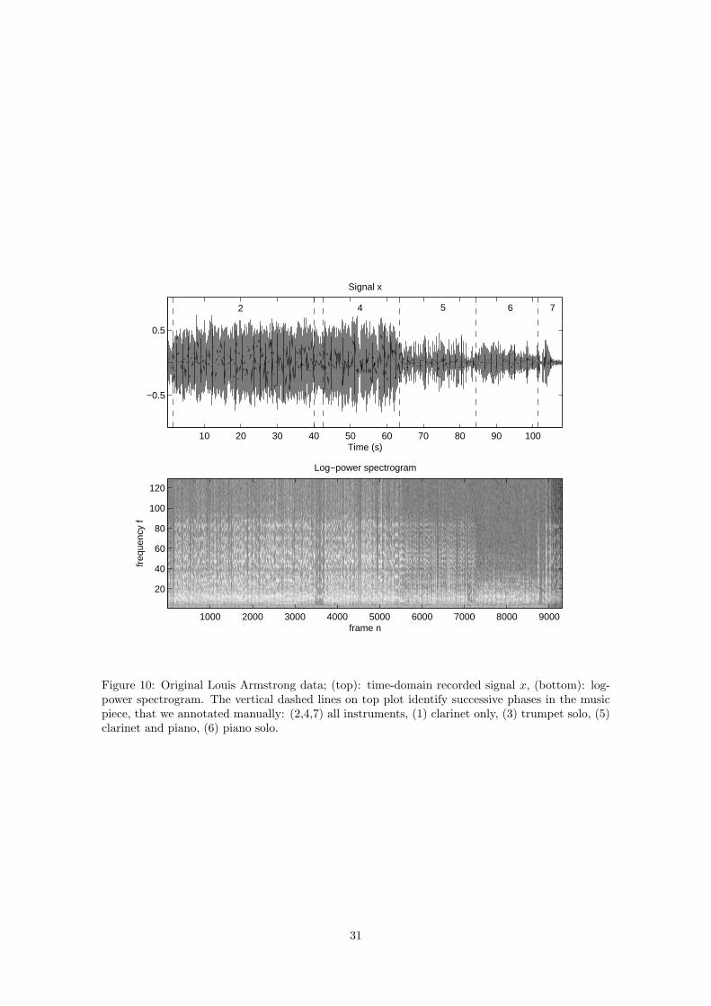
We address the decomposition of a 108 seconds-long music excerpt from My Heart (Will AlwaysLead Me Back To You) recorded by Louis Armstrong and His Hot Five in the twenties. The bandfeatures (to our best hearing) a trumpet, a clarinet, a trombone, a piano and a double bass. Thedata is original unprocessed mono material containing substantial noise. The signal was downsam-pled to νs = 11025 kHz, yielding T = 1191735 samples. The STFT X of x was computed using asinebell analysis window of length L = 256 (23 ms) with 50 % overlap between two frames, leadingto N = 9312 frames and F = 129 frequency bins. The time-domain signal x and its log-powerspectrogram are represented on figure 10.

We applied EUC-NMF, KL-NMF, IS-NMF/MU and IS-NMF/EM to V = |X|.2, as well as aregularized version of IS-NMF, as described in Section 5. We used the inverse-Gamma Markovchain prior (48) with α arbitrarily set to 10. We will refer to this algorithm as “IS-NMF/IG”.Among many trials, this value of α provided a good trade-off between smoothness of the componentreconstructions and adequacy of the components with data. Experiments with the Gamma Markovchain prior (48) did not lead to significant differences in the results and are not reported here.

The number of components K was arbitrarily set to 10. All five algorithms were run forniter = 5000 iterations and were initialized with same random values. For comparison, we havealso applied KL-NMF to the magnitude spectrogram |X| with component reconstruction (24), asthis can be considered state of the art methodology for NMF-based single-channel audio sourceseparation (Virtanen, 2007).

6.2 Results and discussion

For sake of conciseness we here only display the decomposition obtained with IS-NMF/IG, seefigure 12, because it leads to the best results as far as our audio restoration task is concerned,but we stress that all decompositions and component reconstructions obtained from all NMFalgorithms are available online at (Companion Web Site). Figure 12 displays the estimated basisfunctions W in log-scale on the left, and represents on the right the time-domain signal componentsreconstructed from Wiener filtering.

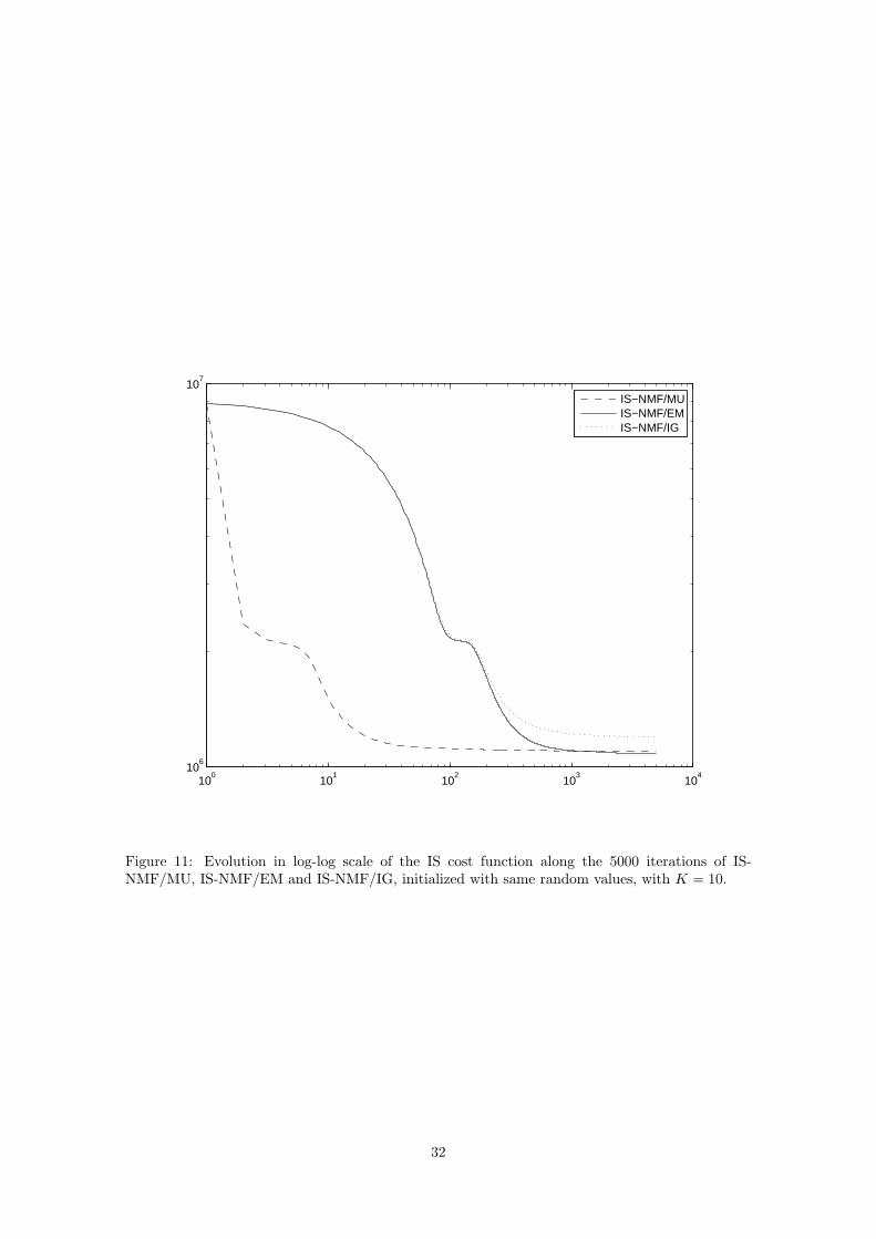
Figure 11 displays the evolution of the IS cost along the 5000 iterations with IS-NMF/MU,IS-NMF/EM and IS-NMF/IG. In this case, IS-NMF/EM achieves a lower cost than IS-NMF/MU.The run times of 1000 iterations of the algorithms were respectively, EUC-NMF: 1.9 min, KL-NMF: 6.8 min, IS-NMF/MU: 8.7 min, IS-NMF/EM: 23.2 min and IS-NMF/IG: 32.2 min.

The comparison of the decompositions obtained with the three cost functions (Euclidean, KLand IS), through visual inspection of W and listening of the components ck, shows again that theIS divergence leads to the most interpretable results. In particular, some of the columns of matrixW produced by all three IS-NMF algorithms have a clear pitched structure, which indicates thatsome notes have been extracted. Furthermore, one of the components captures the noise in therecording. Discarding this component from the reconstruction of x yields satisfying denoising (thisis particularly noticeable during the piano solo, where the input SNR is high). Very surprisingly,most of the rhythmic accompaniment (piano and double bass) is isolated in a single component(component 1 of IS-NMF/MU, component 2 of IS-NMF/EM and IS-NMF/IG), though its spectralcontent is clearly nonstationary. A similar effect happens with IS-NMF/IG and the trombone,which is mostly contained by component 7.

While we do not have a definite explanation for this, we believe that this is a happy consequenceof Wiener reconstruction. Indeed the Wiener component reconstruction is only seen as a set of Kmasking filters applied to xn(f), so that it does not constrain the spectrum of component k to beexactly wk, like the reconstruction method (24) does. So if one assumes that the NMF model (16)adequately captures some of the sound entities present in the mix (in our case that would be thepreponderant notes or chords and the noise), then the other entities are bound to be relegated inremaining components, by conservativity of the decomposition x =

∑Kk=1 ck.

As anticipated, the addition of frame-persistency constraints with IS-NMF/IG impacts the

17

learnt basis W. In particular, some of the components exhibit a more pronounced pitch structure.But more importantly, the regularization yields more pleasant sound reconstructions, this is par-ticularly noticeable when listening to the accompaniment component obtained from IS-NMF/MU(component 1) or IS-NMF/EM (component 2) on the one side and from IS-NMF/IG (component2) on the other side. Note also that in every case the sound quality of Wiener reconstructions isfar better that state of the art KL-NMF of |X| and ad-hoc reconstruction (24).

To conclude this study, we provide online a restored version of the original recording, producedfrom the IS-NMF/IG decomposition. This is to our best knowledge the first use of NMF in areal-case audio restoration scenario. The restoration includes denoising (by discarding component9, which is regarded as noise) and upmixing. A stereo mix is produced by dispatching parts of eachcomponent to left and right channels, hence simulating directions of arrival. As such, we manuallycreated a mix where the components are arranged from 54o left to 54o right, such that the windinstruments (trumpet, clarinet, trombone) are placed left and the stringed instruments (piano,double bass) are placed right. While this stereo mix does render a sensation of spatialization weemphasize that its quality could undoubtedly be improved with appropriate sound engineeringskills.

The originality of our restoration approach lays in 1) the joint noise removal and upmix (asopposed to a suboptimal sequential approach) and 2) the genuine content-based remastering, asopposed to standard techniques based, e.g, on phase delays and/or equalization.

7 Conclusions

We have presented modelling and algorithmic aspects of NMF with the Itakura-Saito divergence.On the modelling side, we wish to bring out the following three features of IS-NMF that have beendemonstrated in this paper;

1) IS-NMF is underlain by a statistical model of superimposed Gaussian components,

2) this model is relevant to the representation of audio signals,

3) this model can accommodate regularization constraints through Bayesian approaches.

On the algorithmic side, we have proposed a novel type of NMF algorithm, IS-NMF/EM, de-rived from SAGE, a variant of the EM algorithm. The convergence of this algorithm to a stationarypoint of the cost function DIS(V|WH) is guaranteed by property of EM. This new algorithm wascompared to an existing algorithm, IS-NMF/MU, whose convergence is not proved, though ob-served in practice. This article also reports an experimental comparative study of the standardEUC-NMF and KL-NMF algorithms, together with the two described IS-NMF algorithms, appliedto a given data set (a short piano sequence), with various random initializations and model orders.Such a furnished experimental study was to our best knowledge not yet available. This articlealso reports a proof of concept of the use of IS-NMF for audio restoration, with a real example.Finally, we also believe to have shed light on the statistical implications of NMF with all of threecost functions.

We have shown how smoothness constraints on W and H can easily be handled in a Bayesiansetting with IS-NMF. As such, we have shown how Markov chains prior structures can improveboth the auditory quality of the component reconstructions and the interpretability of the basiselements. The Bayesian setting opens doors to even more elaborate prior structures that can betterfit the specificities of data. For music signals we believe that two promising lines of research layin 1) the use of switching state models for the rows of H that explicitly model the possibility forhkn to be strictly zero with a certain prior probability (and time persistency could be favored bymodelling the state sequence with a discrete Markov chain), and 2) the use of models that explicitlytake into account the pitched structure of some of the columns of W, and where the fundamentalfrequency could act as a model parameter. These models fit into the problem of object-basedrepresentation of sound, which is an active area of research in the music information retrieval and

18

auditory scene analysis communities.

The experiments in this paper illustrate the slow convergence of the described NMF algo-rithms. The slow convergence of NMF algorithms with multiplicative gradient structure has beenpointed out in other papers, e.g (Berry et al., 2007; Lin, 2007). The proposed IS-NMF/EM doesnot improve on this issue, but its strength is to offer enough flexibility to accommodate Bayesianapproaches. Other types of NMF algorithms, based for example on projected gradient or quasi-Newton methods, have recently been designed to improve convergence of NMF with the Euclideandistance (Berry et al., 2007; Lin, 2007). Such methods are also expected to perform well in thecase of IS-NMF.

Key issues that still need to be resolved in NMF concern identifiability and order selection. Arelated issue is the investigation into the presence of local minima in the cost functions, and waysto avoid them. In that matter, Markov chain Monte Carlo (MCMC) sampling techniques could beused as a diagnostic tool to better understand the topography of the criteria to minimize. While itis not clear whether these techniques can be applied to EUC-NMF or KL-NMF, they can readily beapplied to IS-NMF, using its underlain Gaussian composite structure the same way IS-NMF/EMdoes. As to the avoidance of local minima, techniques inheriting from simulated annealing couldbe applied with IS-NMF, either in MCMC or EM inference.

Regarding order selection, usual criteria such as the Bayesian information criterion (BIC) orAkaike’s criterion (see, e.g., Stoica and Selen (2004)) cannot be directly applied to IS-NMF, becausethe number of parameters (F K + KN) is not constant wrt the number of observations N . Thisfeature breaks the validity of the assumptions in which these criteria have been designed. As such,a final promising line of research concerns the design of methods characterizing p(V|W) insteadof p(V|W,H), treating H as a latent variable, like in independent component analysis (MacKay,1996; Lewicki and Sejnowski, 2000). Besides allowing for model order selection, such approacheswould lead to more reliable estimation of the basis W.

A Standard distributions

Proper complex Gaussian Nc (x|µ,Σ) = |πΣ|−1 exp−(x− µ)H Σ−1 (x− µ)Poisson P(x|λ) = exp(−λ) λ

x

x!

Gamma G(u|α, β) = βα

Γ(α) uα−1 exp(−β u), u ≥ 0

inv-Gamma IG(u|α, β) = βα

Γ(α) u−(α+1) exp(−βu ), u ≥ 0

The inverted-Gamma distribution is the distribution of 1/X when X is Gamma distributed.

B Derivations of the SAGE algorithm

In this appendix we detail the derivations leading to Algorithm 2. The functions involved in thedefinition of QML

k (θk|θ′), given by equation (33), can be derived as follows. The hidden-data minuslog likelihood writes

− log p(Ck|θk) = −N∑n=1

F∑f=1

logNc(ck,fn|0, hkn wfk) (53)

c=N∑n=1

F∑f=1

log (wfk hkn) +|ck,fn|2

wfk hkn. (54)

Then, the hidden-data posterior is obtained through Wiener filtering, yielding

p(Ck|X,θ) =N∏n=1

F∏f=1

Nc(ck,fn|µpostk,fn, λpostk,fn), (55)

19

with µpostk,fn and λpostk,fn given by equations (34) and (35). The E-step is performed by taking theexpectation of (54) wrt the hidden-data posterior, leading to

QMLk (θk|θ′)

c=N∑n=1

F∑f=1

log (wfk hkn) +|µpostk,fn

′|2 + λpostk,fn

′

wfk hkn(56)

c=N∑n=1

F∑f=1

dIS(|µpostk,fn

′|2 + λpostk,fn

′ | wfk hkn). (57)

The M-step thus amounts to minimizing DIS(V′k |wk hk) wrt to wk ≥ 0 and hk ≥ 0, as stated inSection 3.2.

Acknowledgement

The authors acknowledge Roland Badeau, Olivier Cappe, Jean-Francois Cardoso, Maurice Charbitand Alexey Ozerov for discussions related to this work. Many thanks to Gael Richard for com-ments and suggestions about this manuscript and to Simon Godsill for helping us with the LouisArmstrong original data.

References

S. A. Abdallah and M. D. Plumbley. Polyphonic transcription by nonnegative sparse coding ofpower spectra. In 5th Internation Symposium Music Information Retrieval (ISMIR’04), pages318–325, Barcelona, Spain, Oct. 2004.

L. Benaroya, R. Gribonval, and F. Bimbot. Non negative sparse representation for Wiener basedsource separation with a single sensor. In Proc. IEEE International Conference on Acoustics,Speech and Signal Processing (ICASSP’03), pages 613–616, Hong Kong, 2003.

L. Benaroya, R. Blouet, C Fevotte, and I. Cohen. Single sensor source separation using multiple-window STFT representation. In Proc. International Workshop on Acoustic Echo and NoiseControl (IWAENC’06), Paris, France, Sep. 2006.

M. W. Berry, M. Browne, A. N. Langville, V. P. Pauca, and R. J. Plemmons. Algorithms andapplications for approximate nonnegative matrix factorization. Computational Statistics & DataAnalysis, 52(1):155–173, Sep. 2007.

N. Bertin, R. Badeau, and G. Richard. Blind signal decompositions for automatic transcription ofpolyphonic music: NMF and K-SVD on the benchmark. In Proc. International Conference onAcoustics, Speech and Signal Processing (ICASSP’07), 2007.

A. Cichocki, R. Zdunek, and S. Amari. Csiszar’s divergences for non-negative matrix factorization:Family of new algorithms. In 6th International Conference on Independent Component Analysisand Blind Signal Separation, pages 32–39, Charleston SC, USA, 2006.

Companion Web Site. http://www.tsi.enst.fr/∼fevotte/Samples/is-nmf.

I. S. Dhillon and S. Sra. Generalized nonnegative matrix approximations with Bregman divergences.Advances in Neural Information Processing Systems, 19, 2005.

K. Drakakis, S. Rickard, R. de Frein, and A. Cichocki. Analysis of financial data using non-negativematrix factorization. International Journal of Mathematical Sciences, 6(2), June 2007.

S. Eguchi and Y. Kano. Robustifying maximum likelihood estimation. Technical report, Instituteof Statistical Mathematics, June 2001. Research Memo. 802.

M. Feder and E. Weinstein. Parameter estimation of superimposed signals using the EM algorithm.IEEE Transactions on Acoustics, Speech, and Signal Processing, 36(4):477–489, Apr. 1988.

20

J. A. Fessler and A. O. Hero. Space-alternating generalized expectation-maximization algorithm.IEEE Transactions on Signal Processing, 42(10):2664–2677, Oct. 1994.

R. M. Gray, A. Buzo, A. H. Gray, and Y. Matsuyama. Distortion measures for speech processing.IEEE Transactions on Acoustics, Speech, and Signal Processing, 28(4):367–376, Aug. 1980.

F. Itakura and S. Saito. Analysis synthesis telephony based on the maximum likelihood method.In Proc 6th International Congress on Acoustics, pages C–17 – C–20, Tokyo, Japan, Aug. 1968.

R. Kompass. A generalized divergence measure fon nonnegative matrix factorization. NeuralComputation, 19(3):780–791, 2007.

D. D. Lee and H. S. Seung. Algorithms for non-negative matrix factorization. In Advances inNeural and Information Processing Systems 13, pages 556–562, 2001.

D. D. Lee and H. S. Seung. Learning the parts of objects with nonnegative matrix factorization.Nature, 401:788–791, 1999.

M. S. Lewicki and T. J. Sejnowski. Learning overcomplete representations. Neural Computation,12:337–365, 2000.

C.-J. Lin. Projected gradient methods for nonnegative matrix factorization. Neural Computation,19:2756–2779, 2007.

D. MacKay. Maximum likelihood and covariant algorithms for independent component analysis.http://www.inference.phy.cam.ac.uk/mackay/ica.pdf, 1996. Unpublished.

A. Ozerov, P. Philippe, F. Bimbot, and R. Gribonval. Adaptation of Bayesian models for single-channel source separation and its application to voice/music separation in popular songs. IEEETransactions on Audio, Speech, and Language Processing, 15(5):1564–1578, Jul. 2007.

M. D. Plumbley, S. A. Abdallah, T. Blumensath, and M. E. Davies. Sparse representations ofpolyphonic music. Signal Processing, 86(3):417–431, Mar. 2006.

P. Smaragdis. Convolutive speech bases and their application to speech separation. IEEE Trans-actions on Audio, Speech, and Language Processing, 15(1):1–12, Jan. 2007.

P. Smaragdis and J. C. Brown. Non-negative matrix factorization for polyphonic music tran-scription. In IEEE Workshop on Applications of Signal Processing to Audio and Acoustics(WASPAA), Oct. 2003.

P. Stoica and Y. Selen. Model-order selection: a review of information criterion rules. IEEE SignalProcessing Magazine, 21(4):36–47, Jul. 2004.

E. Vincent, N. Bertin, and R. Badeau. Two nonnegative matrix factorization methods forpolyphonic pitch transcription. In Proc. Music Information Retrieval Evaluation eXchange(MIREX), 2007.

T. Virtanen. Monaural sound source separation by non-negative matrix factorization with tem-poral continuity and sparseness criteria. IEEE Transactions on Audio, Speech and LanguageProcessing, 15(3):1066–1074, Mar. 2007.

T. Virtanen, A. T. Cemgil, and S. Godsill. Bayesian extensions to non-negative matrix factorisationfor audio signal modelling. In Proc. International Conference on Acoustics, Speech and SignalProcessing (ICASSP’08), pages 1825–1828, Las Vegas, Apr. 2008.

S. S. Young, P. Fogel, and D. Hawkins. Clustering Scotch whiskies using non-negative matrixfactorization. Joint Newsletter for the Section on Physical and Engineering Sciences and theQuality and Productivity Section of the American Statistical Association, 14(1):11–13, June 2006.

21

0.5 1 1.5 2 2.5 30

0.2

0.4

0.6

0.8

1

1.2

1.4

1.6

1.8

2

EUCKLIS

Figure 1: Euclidean, KL and IS costs d(x|y) as a function of y and for x = 1. The Euclideanand KL divergences are convex on (0,∞). The IS divergence is convex on (0, 2x] and concave on[2x,∞).

22

���� ���� ���� ����� ����� �

2 4 6 8 10 12 14

−0.6

−0.4

−0.2

0

0.2

0.4

Signal x

Time (s)

Log−power spectrogram

frame n

freq

uenc

y f

100 200 300 400 500 600

100

200

300

400

500

Figure 2: Three representations of data; (top): original score, (middle): time-domain recordedsignal x, (bottom): log-power spectrogram log |X|.2. The four notes read D[

4 (pitch 61), F4 (pitch65), A[4 (pitch 68) and C5 (pitch 72). They all together form a D[ major seventh chord. In therecorded interpretation the third chord is slightly out of tempo.

23

0 2 4 6 8 100

5

10

15x 10

7 (a) EUC−NMF

0 2 4 6 8 100

1

2

3

4x 10

5 (b) KL−NMF

0 2 4 6 8 101.5

2

2.5

3

3.5

4

4.5x 10

5 (c) IS−NMF/MU

0 2 4 6 8 101.5

2

2.5

3

3.5

4

4.5x 10

5 (d) IS−NMF/EM

Figure 3: Cost values after 5000 iterations, obtained from 10 different random initializations. (a):Euclidean distance, (b): KL divergence, (c): IS divergence (using IS-NMF/MU), (d): IS divergence(using IS-NMF/EM). On each plot, the solid line connects all minimum cost values while the dashedline connects all maximum cost values.

24

100

102

107

108

109

EUC−NMF runs

100

102

105

106

107

KL−NMF runs

100

102

106

IS−NMF/MU runs

100

102

106

IS−NMF/EM runs

Figure 4: Evolution in log-log scale of the cost functions along the 5000 iterations of all 10 runs ofthe 4 algorithms, in the specific case K = 6.

25

−10

−5

0KL−NMF

0

500

1000

KL−NMF

−10

−5

0

0

5000

−10

−5

0

0

2000

4000

−10

−5

0

0

500

100 200 300 400 500−10

−5

0

frequency f0 200 400 600

0

1000

2000

frame n

Figure 5: KL-NMF with K = 5. Pitch estimates: [61 65 68 72.2 0]. Left : columns of W (log10

scale). Right : rows of H.

26

−10

−5

0EUC−NMF

0

1000

EUC−NMF

−10

−5

0

0

5000

−10

−5

0

0

5000

−10

−5

0

0

2000

4000

−10

−5

0

0

500

100 200 300 400 500−10

−5

0

frequency f0 200 400 600

0

1000

2000

frame n

Figure 6: EUC-NMF with K = 6. Pitch estimates: [61 65 65.4 68 72 0]. Left : columns of W(log10 scale). Right : rows of H.

27

−10

−5

0IS−NMF/MU

0

5000

IS−NMF/MU

−10

−5

0

0

10000

−10

−5

0

05000

10000

−10

−5

0

0

5000

−10

−5

0

012

x 104

100 200 300 400 500−10

−5

0

frequency f0 200 400 600

024

frame n

Figure 7: IS-NMF/MU with K = 6. Pitch estimates: [61 65 68 72 0 0]. Left : columns of W(log10 scale). Right : rows of H.

28

−10

−5

0IS−NMF/EM

0

10000

IS−NMF/EM

−10

−5

0

012

x 105

−10

−5

0

012

x 104

−10

−5

0

0

2000

−10

−5

0

0

50

100 200 300 400 500−10

−5

0

frequency f0 200 400 600

024

frame n

Figure 8: IS-NMF/EM with K = 6. Pitch estimates: [61 65 68 72 0 0]. Left : columns of W (log10

scale). Right : rows of H.

29

0 0.5 1 1.5 2 2.5 3 3.5 4 4.5 50

0.5

1

1.5

2

2.5

3

inverse−GammaGamma

α=50

α=5

Figure 9: Prior pdfs IG(hkn|α−1, α hk(n−1)) (solid line) and G(hkn|α+1, α/hk(n−1)) (dashed line),for hk(n−1) = 1 and for α = {5, 50}.

30

10 20 30 40 50 60 70 80 90 100

−0.5

0.5

Signal x

Time (s)

Log−power spectrogram

frame n

freq

uenc

y f

1000 2000 3000 4000 5000 6000 7000 8000 9000

20

40

60

80

100

120

52 4 6 7

Figure 10: Original Louis Armstrong data; (top): time-domain recorded signal x, (bottom): log-power spectrogram. The vertical dashed lines on top plot identify successive phases in the musicpiece, that we annotated manually: (2,4,7) all instruments, (1) clarinet only, (3) trumpet solo, (5)clarinet and piano, (6) piano solo.

31

100

101

102

103

104

106

107

IS−NMF/MUIS−NMF/EMIS−NMF/IG

Figure 11: Evolution in log-log scale of the IS cost function along the 5000 iterations of IS-NMF/MU, IS-NMF/EM and IS-NMF/IG, initialized with same random values, with K = 10.

32

−6−4−2

IS−NMF/IG

−0.50

0.5IS−NMF/IG

−6−4−2

−0.50

0.5

−5−4−3−2−1

−0.50

0.5

−5−4−3−2−1

−0.50

0.5

−5−4−3−2−1

−0.50

0.5

−5−4−3−2−1

−0.50

0.5

−6−4−2

−0.50

0.5

−4−2

−0.50

0.5

−5−4−3−2−1

−0.50

0.5

20 40 60 80 100 120−4−2

frequency f

−0.50

0.5

time

Figure 12: Decomposition of Louis Armstrong music data with IS-NMF/IG. Left : columns of W(log10 scale). Right : reconstructed components ck; the x-axis ticks correspond to the temporalsegmentation border lines displayed with signal x on figure 10.

33

K 1 2 3 4 5 10 O(.)EUC-NMF 17 18 20 24 27 37 4FKN + 2K2(F +N)KL-NMF 90 90 92 100 107 117 8FKNIS-NMF/MU 127 127 129 135 138 149 12FKNIS-NMF/EM 81 110 142 171 204 376 12FKN

Table 1: Run times in seconds of 1000 iterations of the NMF algorithms applied to the pianodata, implemented in Matlab on a 2.16 GHz Intel Core 2 Duo iMac with 2 GB RAM. The runtimes include the computation of the cost function at each iteration (for possible convergencemonitoring). The last column shows the algorithm complexities per iteration, expressed in numberof flops (addition, soustraction, multiplication, division). The complexity of EUC-NMF assumesK < F,N .

34

inverse-Gamma Markov chainp2 p1 p0

hk1 (α+ 1)/hk2 F − α+ 1 −F hMLk1

hkn (α+ 1)/hk(n+1) F + 1 −F hMLkn − (α+ 1)hk(n−1)

hkN 0 F + α+ 1 −F hMLkN − (α+ 1)hk(N−1)

Gamma Markov chainp2 p1 p0

hk1 0 F + α+ 1 −F hMLk1 − (α− 1)hk2

hkn (α− 1)/hk(n−1) F + 1 −F hMLkn − (α− 1)hk(n+1)

hkN (α− 1)/hk(N−1) F − α+ 1 −F hMLkN

Table 2: Coefficients of the order 2 polynomial to solve in order to update hkn in Bayesian IS-NMFwith a Markov chain prior. hML

kn denotes the ML update, given by equation (39).

35

Dépôt légal : 2008 – 2ème trimestre Imprimé à l’Ecole Nationale Supérieure des Télécommunications – Paris

ISSN 0751-1345 ENST D (Paris) (France 1983-9999)

TELECOM ParisTech

Institut TELECOM - membre de ParisTech

46, rue Barrault - 75634 Paris Cedex 13 - Tél. + 33 (0)1 45 81 77 77 - www.telecom-paristech.frfr

Département TSI

©

Inst

itut

TE

LE

CO

M -

TE

LE

CO

M P

ari

sT

ech

20

08