Separating Doubly Nonnegative andCompletely Positive Matrices

Hongbo Dong∗ and Kurt Anstreicher†

March 8, 2010

Abstract

The cone of Completely Positive (CP) matrices can be used to exactly formulate avariety of NP-Hard optimization problems. A tractable relaxation for CP matrices isprovided by the cone of Doubly Nonnegative (DNN) matrices; that is, matrices thatare both positive semidefinite and componentwise nonnegative. A natural problem inthe optimization setting is then to separate a given DNN but non-CP matrix from thecone of CP matrices. We describe two different constructions for such a separation thatapply to 5×5 matrices that are DNN but non-CP. We also describe a generalization thatapplies to larger DNN but non-CP matrices having block structure. Computationalresults illustrate the applicability of these separation procedures to generate improvedbounds on difficult problems.

1 Introduction

Let Sn denote the set of n × n real symmetric matrices, S+n denote the cone of n × n real

symmetric positive semidefinite matrices and Nn denote the cone of symmetric nonnegativen×n matrices. The cone of doubly nonnegative (DNN) matrices is then Dn = S+

n ∩Nn. Thecone of completely positive (CP) n × n matrices, denoted Cn, consists of all matrices thatcan be written in the form AAT where A is an n× k nonnegative matrix. The dual cone C∗nis the cone of n × n copositive matrices, that is, matrices X ∈ Sn such that yTXy ≥ 0 forevery y ∈ <+

n .The CP cone is of interest in optimization due to the fact that a variety of NP-Hard

problems can be represented as linear optimization problems over Cn; see [Bur09] and refer-ences therein. On the other hand, the DNN cone provides a tractable relaxation Cn ⊂ Dnsince linear optimization over Dn can be performed using software for self-dual cones suchas SeDuMi [Stu99]. A natural problem in the optimization setting is then to separate agiven DNN but non-CP matrix from the CP cone. Since Dn = Cn for n ≤ 4 [BSM03], thisseparation problem is of interest for matrices with n ≥ 5. The separation problem for n = 5

∗Department of Applied Mathematics and Computational Sciences, University of Iowa, Iowa City, IA52242. email:hondong@math.uiowa.edu†Corresponding author. Department of Management Sciences, University of Iowa, Iowa City, IA 52242.

email:kurt-anstreicher@uiowa.edu

1

was first considered in [BAD09]. Following the terminology of [BAD09], we say that an n×nmatrix is bad if X ∈ Dn \Cn, and extremely bad if X is a bad extreme ray of Dn. In [BAD09]it is shown that if X ∈ D5 is extremely bad, then X can be constructively separated fromC5 using a “cut” matrix V ∈ C∗5 that has V •X < 0.

In this paper we describe new separation procedures that apply to matrices X ∈ Dn \Cn.In Section 2, we generalize the separation procedure from [BAD09] to apply to a broaderclass of matrices X ∈ D5 \ C5 than the extremely bad matrices considered in [BAD09].As in [BAD09], the cut matrix that is constructed is a transformation of the Horn matrixH ∈ C∗5 \D∗5. We also show that these “transformed Horn cuts” induce 10-dimensional facesof the 15-dimensional cone C5. In Section 3 we describe an even more general separationprocedure that applies to any matrix X ∈ D5\C5 that is not componentwise strictly positive.The cut generation procedure in this case relies on the solution of a conic optimizationproblem. In Section 4 we describe separation procedures motivated by the procedure ofSection 3 that apply to matrices in Dn \ Cn, n > 5 having block structure. In all cases, thegoal is to find a copositive V ∈ C∗n that separates X from Cn via V • X < 0. In Section 5we numerically apply the separation procedures developed in Sections 2-4 to selected testproblems.

To date, most of the literature concerning the use of CP matrices in optimization hasinvolved schemes for approximating the copositive cones C∗n. For example, [BdK02] and[dKP02] describe a hierarchy of cones Krn, r ≥ 0, with K0

n = D∗n and Krn ⊂ Kr+1n ⊂ C∗n.

A different approach to dynamically refining an approximation of C∗n is taken in [BD09].To our knowledge, the only paper other than [BAD09] that considers strengthening theDNN relaxation of a problem posed over CP matrices by generating cuts corresponding tocopositve matrices is [BFL10]. However, the methodology described in [BFL10] is specific toone particular problem (max-clique), while our approach is independent of the underlyingproblem and assumes only that the goal is to obtain a CP solution.

Notation: For X ∈ Sn, we sometimes write X � 0 to mean X ∈ S+n . We use e to denote

a vector of appropriate dimension with each component equal to one, and E = eeT . For avector v ≥ 0,

√v is the vector whose ith component is

√vi. For n × n matrices A and B,

A ◦B denotes the Hadamard product (A ◦B)ij = aijbij, and A •B denotes the matrix innerproduct A •B = eT (A ◦B)e. If a ∈ <n and A is an n× n matrix, then diag(A) is the vectorwhose ith component is aii, while Diag(a) is the diagonal matrix with diag(Diag(a)) = a.For X ∈ Sn, G(X) denotes the undirected graph with vertex set {1, 2, . . . , n} and edge set{{i 6= j} : xij 6= 0}. We use Co{ · } to denote the convex hull of a set.

2 Separation based on the Horn matrix

In this section we describe a procedure for separating a bad 5 × 5 matrix from C5 thatgeneralizes the separation procedure for extremely bad matrices in [BAD09]. Recall thatfrom [BAD09], the class of extremely bad matrices (extreme rays of D5 that are not in C5) is

E5 := {X ∈ D5 : rank(X) = 3 and G(X) is a 5-cycle}.

Note that when G(X) is a 5-cycle, every vertex in G(X) has degree equal to two. We willgeneralize the procedure of [BAD09] to apply to the case where rank(X) = 3 and G(X) hasat least one vertex with degree two.

2

Our construction utilizes several results from [BX04] regarding matrices in D5 \ C5 of theform

X =

X11 α1 α2

αT1 1 0αT2 0 1

, (1)

where X11 ∈ D3. Following the notation of [BX04], for a matrix X ∈ D5 of the form (1), letC denote the Schur complement C = X11 − α1α

T1 − α2α

T2 . Let µ(C) denote the number of

negative components above the diagonal in C, and if µ(C) > 0 define

λ4 = min1≤i<j≤3

{xi4xj4−cij

∣∣∣∣ cij < 0

}, λ5 = min

1≤i<j≤3

{xi5xj5−cij

∣∣∣∣ cij < 0

}. (2)

It is shown in [BX04, Theorem 2.5] that X ∈ C5 if µ(C) > 1 and λ4 + λ5 ≥ 1, and in[BX04, Theorem 3.1] that X ∈ C5 if µ(C) 6= 2. Thus for a matrix X ∈ D5 of the form (1),X ∈ D5 \ C5 implies that µ(C) = 2 and λ4 + λ5 < 1. Finally, when rank(X) = 3, it is shownin [BX04, Theorem 4.2] that these conditions are also sufficient to have X ∈ D5 \ C5. Forconvenience we repeat this result here.

Theorem 1. [BX04, Theorem 4.2] Assume that X ∈ D5 has the form (1), with rank(X) = 3.Then X ∈ D5 \ C5 if and only if µ(C) = 2 and λ4 + λ5 < 1, where λ4 and λ5 are given by(2).

As in [BAD09], the separation procedure developed here is based on a transformation ofthe well-known Horn matrix [HJ67],

H :=

1 −1 1 1 −1−1 1 −1 1 1

1 −1 1 −1 11 1 −1 1 −1−1 1 1 −1 1

∈ C∗5 \ D∗5.Theorem 2. Suppose that X ∈ D5 \ C5 has rank(X) = 3, and G(X) has a vertex of degreetwo. Then there exists a permutation matrix P and a diagonal matrix Λ with diag(Λ) > 0such that

PΛHΛP T •X < 0.

Proof. To begin, consider a transformation of X of the form

X = ΣQXQTΣ, (3)

where Σ is a diagonal matrix with diag(Σ) > 0 and Q is a permutation matrix. Then Xsatisfies the conditions of the theorem if and only if X does. Moreover,

PΛHΛP T • X = PΛHΛP T • ΣQXQTΣ

= PΛHΛP T • Σ(PP T )QXQT (PP T )Σ

= QTP (P TΣP )ΛHΛ(P TΣP )P TQ •X= P ΛHΛP T •X,

3

where P = QTP and Λ = (P TΣP )Λ. It follows that if we apply an initial transformation ofthe form (3) and show that the theorem holds for X, then it also holds for X. Below we willcontinue to refer to such a transformed matrix as X rather than X to reduce notation.

Note that diag(X) > 0, because otherwise X � 0 implies that the only nonzero blockin X is a 4 × 4 DNN matrix, and therefore X ∈ C5. Since G(X) has a vertex of degree 2,after applying a suitable permutation we may assume that x45 = x15 = 0, x25 > 0, x35 > 0.The assumption that X ∈ D5 \ C5 then implies that x14 > 0, since otherwise it is easy tosee that G(X) would contain no 5-cycle, implying X ∈ C5 [BSM03]. Let C denote the Schurcomplement C = X11 − α1α

T1 − α2α

T2 . By Theorem 1, C has exactly two negative entries

above the diagonal, so at least one of c13 and c23 must be negative. If necessary interchangingrow/column 2 and 3, we can assume that c13 < 0. After applying a suitable diagonal scalingwe may therefore assume that X has the form (1), with α1 = (1, u, v)T and α2 = (0, 1, 1)T .

The fact that rank(X) = 3 implies that rank(C) = 1, and X � 0 implies that C � 0.Since c13 < 0, it follows that there are scalars x > 0, y > 0, z > 0 so that C has one of thefollowing forms:

C =

xy−z

xy−z

T

or C =

x−y−z

x−y−z

T

.

We next show that in fact the second case is impossible under the assumptions of the theorem.Assume that

C =

x−y−z

x−y−z

T

, so X11 =

x2 + 1 u− xy v − xzu− xy y2 + u2 + 1 yz + uv + 1v − xz yz + uv + 1 z2 + v2 + 1

. (4)

By Theorem 1, λ4 + λ5 < 1, where λ4 and λ5 are defined as in (2). Obviously λ5 = 0, andλ4 = min{ u

xy, vxz}. But λ4 = u

xy< 1 ⇒ −xy + u < 0 ⇒ x12 < 0, which is impossible since

X ∈ D5. Assuming that λ4 = vxy< 1 leads to a similar contradiction x13 < 0, and therefore

(4) cannot occur. We may therefore conclude that

C =

xy−z

xy−z

T

, so X11 =

x2 + 1 xy + u v − xzxy + u y2 + u2 + 1 uv − yz + 1v − xz uv − yz + 1 z2 + v2 + 1

. (5)

Again λ5 = 0, and now λ4 = min{ vxz, uvyz}. Then λ4 = v

xz< 1⇒ x13 < 0, which is impossible,

so we must have λ4 = uvyz< 1.

Let T be the permuted Horn matrix

T := PHP T =

1 −1 1 −1 1−1 1 1 1 −1

1 1 1 −1 −1−1 1 −1 1 1

1 −1 −1 1 1

, where P =

1 0 0 0 00 1 0 0 00 0 0 1 00 0 0 0 10 0 1 0 0

.

Computation using symbolic mathematical software yields

Det (X ◦ T ) = −4x2(yz − uv)2 < 0.

4

Thus X ◦ T is nonsingular, and symbolic software obtains (X ◦ T )−1 = 12(uv−yz)DxMDx,

where Dx = Diag(( 1x, 1, 1, 1

x, 1)T ) and

M =

2uv z y vxy − uxz + 2uv y + zz 0 1 z + vx 1y 1 0 y − ux 1

vxy − uxz + 2uv z + vx y − ux 2(u+ xy)(v − xz) y + z + vx− uxy + z 1 1 y + z + vx− ux 2(1 + uv − yz)

.

By using the inequalities x13 = v− xz ≥ 0, x23 = uv− yz + 1 ≥ 0 and an implied inequalityλ4 < 1 ⇒ yz > uv ≥ uxz ⇒ y > ux, one can easily verify that M ≥ 0 and therefore(X ◦ T )−1 ≤ 0, with at least one strictly negative component in each row.

Finally, define w = −(X ◦ T )−1e > 0, V = Diag(w)T Diag(w) = PΛHΛP T whereΛ = P T Diag(w)P . Then

V •X = Diag(w)T Diag(w) •X = (T ◦ wwT ) •X = wwT • (X ◦ T )

= wT (X ◦ T )w = eT (X ◦ T )−1(X ◦ T )(X ◦ T )−1e = eTw < 0.

In Theorem 2, the condition that G(X) has a vertex with degree 2 implies that G(X) isa “book graph with CP pages.” There exists an algebraic procedure to determine whethera matrix X ∈ Dn with such a graph is in Cn; see [Bar98] or [BSM03, Theorem 2.18]. WhenX is extremely bad, it can be shown that the matrix X ◦ T in the proof of Theorem 2 is“almost copositive,” which implies the facts that X ◦ T is nonsingular and (X ◦ T )−1 ≤ 0[Val89, Theorem 4.1]. However, we have been unable to show that X ◦T is almost copositiveunder the more general assumptions of Theorem 2.

Let V ∈ C∗5 , and consider a cut of the form V •X ≥ 0 that is valid for any X ∈ C5. Fromthe standpoint of eliminating elements of D5 \ C5, it is desirable for the face

F(C5, V ) = {X ∈ C5 : V •X = 0}

to have high dimension. We next show that the cut based on a transformed Horn matrixfrom Theorem 2 induces a 10-dimensional face of the 15-dimensional cone C5. (It is known[DS08] that Cn has an interior in the n(n + 1)/2-dimensional space corresponding to thecomponents of X ∈ Cn on or above the diagonal.)

Theorem 3. Let V = PΛHΛP T , where P is a permutation matrix and Λ is a diagonalmatrix with diag(Λ) > 0. Then dimF(C5, V ) = 10.

Proof. Without loss of generality we may take P = Λ = I, so V = H. The extreme raysof F(C5, H) are then matrices of the form X = xxT , where x ≥ 0 and xTHx = 0, and anyelement of F(C5, H) can be written as a nonnegative combination of such extreme rays. Todetermine dimF(C5, H) we must therefore determine the maximum number of such extremerays that are linearly independent.

For any X = xxT , x ≥ 0 let I(x) = {i : x(i) > 0}. We first consider which sets I(x) arepossible for X = xxT ∈ F(C5, H). It is easy to show that

xTHX = (x1 − x2 + x3 + x4 − x5)2 + 4x2x4 + 4x3(x5 − x4)

= (x1 − x2 + x3 − x4 + x5)2 + 4x2x5 + 4x1(x4 − x5).

5

The fact that H ∈ C∗5 then follows from the fact that for any x ≥ 0, either x4 ≥ x5 orx5 ≥ x4. Moreover, x > 0 and xTHx = 0 would imply x4 = x5 > 0, and therefore x2 = 0,a contradiction, so |I(x)| = 5 is impossible. Similarly |I(x)| = 4 implies that x4 = x5 > 0,and therefore x2 = 0, so (x1 − x2 + x3 + x4 − x5)

2 = (x1 + x3)2 > 0, and xxT /∈ F(C5, H).

Thus |I(x)| = 4 is impossible. Finally |I(x)| = 1 is impossible since diag(H) = e > 0, sothe only possibilities are |I(x)| = 2 and |I(x)| = 3.

Let H+ and X+ be the principal submatrices of H and X = xxT , respectively, corre-sponding to the positive components of x. For |I(x)| = 2, H+ has the form(

1 −1−1 1

)or

(1 11 1

),

and obviously xTHx = 0 is only possible in the first case. It follows that if |I(x)| = 2, thenI(x) is either {1, 2}, {2, 3}, {3, 4}, {4, 5} or {5, 1}, and in each case X+ is a positive multipleof eeT .

Next assume that |I(x)| = 3. Clearly H+ cannot have a row equal to (1, 1, 1), and the3 × 3 principal submatrices of H that do not contain such a row correspond to I(x) equalto {1, 2, 3}, {2, 3, 4}, {3, 4, 5}, {4, 5, 1} and {5, 1, 2}. Consider I(x) = {1, 2, 3}, so

H+ =

1 −1 1−1 1 −1

1 −1 1

.

Since H+ � 0, xTHx = 0 ⇐⇒ H+x+ = 0, where x+ = (x1, x2, x3)T . It is then obvious that

x+ = x2(u, 1, 1− u)T for some 0 < u < 1. The vector t corresponding to the upper triangleof x+(x+)T then has the form

t = (x11, x12, x13, x22, x23, x33)T = x2

2(u2, u, u(1− u), 1, (1− u), (1− u)2)T . (6)

Any vector of the form (6) satisfies the equations

t1 − 2t2 + t4 − t6 = 0

t1 − t2 + t3 = 0

t2 − t4 + t5 = 0.

These equations are linearly independent, so there can be at most 3 linearly independentvectors of the form (6). However, the values u = 0 and u = 1 correspond to two of thematrices X = xxT with |I(x) = 2|, so only one matrix with 0 < u < 1 can be addedwhile maintaining a linearly independent set. The same argument applies for all of the otherpossibilities having |I(x) = 3|, so the maximum possible dimension for F(C5, H) is ten.Finally it can be verified numerically that the five X = xxT with distinct |I(x) = 2|, andfive with distinct |I(x) = 3|, are in fact linearly independent.

As mentioned above, Theorem 2 can be viewed as a generalization of the separation resultfor extremely bad 5 × 5 matrices in [BAD09, Theorem 8]. To make this connection moreexplicit, we can use the fact [BAD09, Section 2] that X ∈ D5 \ C5 is extremely bad if and

6

only if X can be written in the form

X = PΛ

1 β1 0 0 1β1 β2

1 + β22 + 1 β2 0 0

0 β2 1 1 00 0 1 β2

2 + 1 β1β2

1 0 0 β1β2 β21 + 1

ΛP T ,

where Λ is a positive diagonal matrix, P is a permutation matrix and β1, β2 > 0. With asuitable permutation of rows/columns and a slight modification in Λ, this characterizationis equivalent to

X = PΛ

β2

1 + 1 β1β2 0 1 0β1β2 β2

2 + 1 0 0 1

0 0β21

β22

+ 1 + 1β22

β1

β21

1 0 β1

β21 0

0 1 1 0 1

ΛP T ,

corresponding to (5) with u = 0, v = β1

β2, x = β1, y = β2, z = 1

β2. Another interesting special

case where Theorem 2 applies is as follows. Let H be the Horn matrix and consider the faceof D5,

F(D5, H) := {X ∈ D5 : H •X = 0} .

In the optimization context an element of F(D5, H) could arise naturally via the followingsequence. Suppose that an optimization problem posed over D5 has a solution X thatsatisfies the assumptions of Theorem 2 (for example, X is extremely bad). After addinga transformed Horn cut and re-solving, the new solution X ′ (after diagonal scaling andpermutation) would likely be an extreme ray of F(D5, H). Burer (private communication)obtained the following characterization of the extreme rays of F(D5, H).

Theorem 4. Let X be an extreme ray of F(D5, H). Then rank(X) equals 1 or 3. Further,if rank(X) = 3, then G(X) is either a 5-cycle, or a 5-cycle with a single additional chord.

One can characterize the matrices in Theorem 4 using an argument similar to whatis done in [BAD09, Section 2] to characterize extremely bad matrices. The result is that amatrix X ∈ D5 satisfies the conditions of Theorem 4 if and only if there exists a permutationmatrix P , a positive diagonal matrix Λ and β1, β2, β3 > 0, β2 ≤ β1β3, such that

X = PΛ

β2

1 + 1 β1β2 0 1 0

β1β2 β22 + 1 1− β2

β1β30 1

0 1− β2

β1β3

1β23

+ 1 + 1β21β

23

1β3

1

1 0 1β3

1 0

0 1 1 0 1

ΛP T ,

correponding to (5) with u = 0, v = 1β3

, x = β1, y = β2, z = 1β1β3

. Note that such an X isextremely bad if and only if β2 = β1β3.

7

3 Separation based on conic programming

In this section we describe a separation procedure that applies to a broader class of matricesX ∈ D5 \ C5 than the procedure of the previous section. Let X ∈ D5, with at least oneoff-diagonal zero, and assume that diag(X) > 0 since otherwise X ∈ C5 is immediate. Aftera permutation and diagonal scaling, X may be assumed to have the form (1). For such amatrix a useful characterization of X ∈ C5 is given by the following theorem from [BX04].

Theorem 5. [BX04, Theorem 2.1] Let X ∈ D5 have the form (1). Then X ∈ C5 if and onlyif there are matrices A11 and A22 such that X11 = A11 + A22, and(

Aii αiαTi 1

)∈ D4, i = 1, 2.

In [BX04], Theorem 5 is utilized only as a proof mechanism, but we now show that ithas algorithmic consequences as well.

Theorem 6. Assume that X ∈ D5 has the form (1). Then X ∈ D5 \ C5 if and only if thereis a matrix

V =

V11 β1 β2

βT1 γ1 0βT2 0 γ2

such that

(V11 βiβTi γi

)∈ D∗4, i = 1, 2,

and V •X < 0.

Proof. Consider the “CP feasibility problem”

(CPFP) min 2θ

s.t.

(Aii αiαTi 1

)+ θ(I + E) ∈ D4, i = 1, 2

A11 + A22 = X11

θ ≥ 0,

where by assumption αi ≥ 0, i = 1, 2 and X11 ∈ D3. By Theorem 5, X ∈ C5 if and only ifthe solution value in CPFP is zero. Using conic duality it is straightforward to verify thatthe dual of CPFP can be written

(CPDP) max −(V11 •X11 + 2αT1 β1 + 2αT2 β2 + γ1 + γ2)

s.t.

(V11 βiβTi γi

)∈ D∗4, i = 1, 2

(I + E) • V11 + eTβ1 + eTβ2 + γ1 + γ2 ≤ 1.

Moreover CPFP and CPDP both have feasible interior solutions, so strong duality holds.The proof is completed by noting that the objective in CPDP is exactly −V •X.

Suppose that X ∈ D5 \ C5, and V is a matrix that satisfies the conditions of Theorem6. If X ∈ C5 is another matrix of the form (1), then Theorem 5 implies that V • X ≥ 0.However we cannot conclude that V ∈ C∗5 because V • X ≥ 0 only holds for X of the form(1), in particular, x45 = 0. Fortunately, the matrix V can easily be “completed” to obtain acopositive matrix that still separates X from C5.

8

Theorem 7. Suppose that X ∈ D5 \ C5 has the form (1), and V satisfies the conditions ofTheorem 6. Define

V (s) =

V11 β1 β2

βT1 γ1 sβT2 s γ2

.

Then V (s) •X < 0 for any s, and V (s) ∈ C∗5 for s ≥ √γ1γ2.

Proof. The fact that V (s) • X = V • X < 0 is obvious from x45 = 0, and V (s) ∈ C∗5 fors ≥ √γ1γ2 follows immediately from [HJR05, Theorem 1].

Theorems 6 and 7 provide a separation procedure that applies to any X ∈ D5 \ C5 thatis not componentwise strictly positive. In applying Theorem 6 to separate a given X, onecan numerically minimize X • V , where V satisfies the conditions in the theorem and isnormalized via a condition such as I • V = 1 or (I + E) • V = 1. In [BX04, Theorem 6.1]it is claimed that if X ∈ D5 \ C5, X > 0, then there is a simple transformation of X thatproduces another matrix X ∈ D5 \ C5, X 6> 0, suggesting that a separation procedure forX could be based on applying the construction of Theorem 6 to X. However it is shown in[DA09] that in fact [BX04, Theorem 6.1] is false.

4 Separation for matrices with n > 5

Suppose now that X ∈ Dn \ Cn for n > 5. In order to separate X from Cn, we could attemptto apply the procedure in Section 2 or Section 3 to candidate 5× 5 principal submatrices ofX. However, it is possible that all such submatrices are in C5 so that no cut based on a 5×5principal submatrix can be found. In this section we consider extensions of the separationprocedure developed in Section 3 to matrices X ∈ Dn \ Cn, n > 5 having block structure. Inorder to state the separation procedure in its most general form we will utilize the notion ofa CP graph.

Definition 1. Let G be an undirected graph on n vertices. Then G is called a CP graph ifany matrix X ∈ Dn with G(X) = G also has X ∈ Cn.

The main result on CP graphs is the following:

Proposition 1. [KB93] An undirected graph on n vertices is a CP graph if and only if itcontains no odd cycle of length 5 or greater.

Our separation procedure is based on a simple observation for CP matrices of the form

X =

X11 X12 X13 . . . X1k

XT12 X22 0 . . . 0

XT13 0

. . . . . ....

......

. . . . . . 0XT

1k 0 . . . 0 Xkk

, (7)

where k ≥ 3, each Xii is an ni × ni matrix, and∑k

i=1 ni = n.

9

Lemma 1. Suppose that X ∈ Dn has the form (7), k ≥ 3, and let

X i =

(X11 X1i

XT1i Xii

), i = 2, . . . , k.

Then X ∈ Cn if and only if there are matrices Aii, i = 2, . . . , k such that∑k

i=2Aii = X11,and (

Aii X1i

XT1i Xii

)∈ Cn1+ni

, i = 2, . . . , k.

Moreover, if G(X i) is a CP graph for each i = 2, . . . , k, then the above statement remainstrue with Cn1+ni

replaced by Dn1+ni.

Proof. Let N1 = 0, Ni = Ni−1 +ni, i = 2, . . . , k, and Ii = {Ni + 1, . . . , Ni +ni}, i = 1, . . . , k.Then Ii contains the indeces of the rows and columns of X corresponding to Xii. From thestructure of X, it is clear that X ∈ Cn if and only if there are nonnegative vectors aij suchthat

X =k∑i=2

mi∑j=1

aij(aij)T ,

where aijl = 0 for l /∈ I1 ∪ Ii. The lemma follows by deleting the rows and columns of∑mi

j=1 aij(aij)T that are not in I1∪Ii. That Cn1+ni

can be replaced by Dn1+niwhen G(X i) is

a CP graph follows from Definition 1 and the fact that G(Aii) must be a subgraph of G(X11)for each i.

Theorem 8. Suppose that X ∈ Dn \ Cn has the form (7), where G(X i) is a CP graph,i = 2, . . . , k. Then there is a matrix

V =

V11 V12 V13 . . . V1k

V T12 V22 0 . . . 0

V T13 0

. . . . . ....

......

. . . . . . 0V T

1k 0 . . . 0 Vkk

such that (

V11 V1i

V T1i Vii

)∈ D∗n1+ni

, i = 2, . . . , k,

and V •X < 0. Moreover, the matrix

V =

V11 . . . V1k...

. . ....

V T1k . . . Vkk

,

where Vij =√

diag(Vii)√

diag(Vjj)T

, 2 ≤ i 6= j ≤ k, has V ∈ C∗n and V •X = V •X < 0.

Proof. The proof uses an argument very similar to that used to prove Theorems 6 and 7.

10

When n1 = 2, a matrix X satisfying the conditions of Theorem 8 has a book graph withk CP pages, and an algebraic procedure for testing if X ∈ Cn is known [Bar98]. There areseveral situations where we can immediately use Theorem 8 to separate a matrix of the form(7) with X ∈ Dn \ Cn from Cn. One case, corresponding to n1 = 3 and ni = 1, i = 2, . . . , kcan be viewed as a generalization of the separation procedure for a matrix of the form (1) inthe previous section. Assuming that X has no zero diagonal components, after a symmetricpermutation and diagonal rescaling, and setting k ← k − 1, we may assume that such amatrix X has the form

X =

X11 α1 α2 . . . αkαT1 1 0 . . . 0

αT2 0. . . . . .

......

.... . . . . . 0

αTk 0 . . . 0 1

. (8)

Corollary 1. Suppose that X ∈ Dn \ Cn has the form (8), where X11 ∈ D3. Then there is amatrix

V =

(V11 BBT Diag(γ)

)where V11 ∈ D∗3, B = (β1, β2, . . . , βk) and γ ≥ 0 such that(

V11 βiβTi γi

)∈ D∗4, i = 1, 2, . . . , k

and V •X < 0. Moreover, if s =√γ then

V (s) =

(V11 BBT ssT

)∈ C∗n.

Note that in the case where X has the structure (8), the vertices 4, . . . , k + 3 form astable set of size k in G(X). A second case where the structure (7) can immediately be usedto generate a cut separating a matrix X ∈ Dn \ Cn is when ni = 2, i = 1, . . . , k. In this casethe subgraph of G(X) on the vertices 3, . . . , 2k is a matching, and the matrices(

V11 V1i

V T1i Vii

)in Theorem 8 are again all in D∗4.

A second case where block structure can be used to generate cuts for a matrix X ∈ Dn\Cnis when X has the form

X =

I X12 X13 . . . X1k

XT12 I X23 . . . X2k

XT13 XT

23. . . . . .

......

.... . . . . . X(k−1)k

XT1k 0 . . . XT

(k−1)k I

, (9)

where k ≥ 2, each Xij is an ni×nj matrix, and∑k

i=1 ni = n. The structure in (9) correspondsto a partitioning of the vertices {1, 2, . . . , n} into k stable sets in G(X), of size n1, . . . , nk(note that ni = 1 is allowed). In order to succinctly characterize when X ∈ Cn for such amatrix it is convenient to utilize a multi-index vector p ∈ Zk, with components 1 ≤ pi ≤ ni.

11

Lemma 2. Suppose that X ∈ Dn has the structure (9). For each p ∈ Zk with 1 ≤ pi ≤ ni,i = 1 . . . , n, let Xp be the k × k matrix with components

[Xp]ij =

{[Xij]pipj

i 6= j,

api i = j,

where ap ∈ <k. Then X ∈ Cn if and only if there are ap ∈ <k so that Xp ∈ Ck for each p,and ∑

p:pi=j

api = 1

for each i = 1, . . . , k and 1 ≤ j ≤ ni. If in addition G(Xp) is a CP graph for each p, thenthe above statement holds with Dk in place of Ck.

Proof. The proof is similar to that of Lemma 1, but uses the fact that if X has the form(9) and bbT is a rank-one matrix in the CP-decomposition of X, then for each i = 1, . . . , k,bj > 0 for at most one j ∈ I(i) .

Theorem 9. Suppose that X ∈ Dn \ Cn has the form (9), where G(Xp) is a CP graph foreach p ∈ Zk with 1 ≤ pi ≤ ni, i = 1, . . . , k. Then there is a matrix

V =

Diag(γ1) V12 V13 . . . V1k

V T12 Diag(γ2) V23 . . . V2k

V T13 V T

23. . . . . .

......

.... . . . . . V(k−1)k

V T1k 0 . . . V T

(k−1)k Diag(γk)

,

with V •X < 0, such that for every p ∈ Zk with 1 ≤ pi ≤ ni, i = 1, . . . , k, V p ∈ D∗k, where

[V p]ij =

{[Vij]pipj

i 6= j,

γipii = j.

Moreover, the matrix

V =

V11 . . . V1k...

. . ....

V T1k . . . Vkk

,

where Vii =√γi√γiT

, has V ∈ C∗n and V •X = V •X < 0.

Proof. The proof uses an argument very similar to that used to prove Theorems 6 and 7.

To close the section we mention two details regarding the applicability of Lemmas 1 and2 to separate a given X ∈ Dn \ Cn from Cn, via the cuts described in Theorems 8 and 9.First, in practice a given matrix X may have numerical entries that are small but not exactlyzero. In such a case, Lemma 1 or 2 can be applied to a perturbed matrix X, where entriesof X below a specified tolerance are set to zero in X. If a cut V separating X from Cn isfound and the zero tolerance is small, then V •X ≈ V • X < 0, and V is very likely to alsoseparate X from Cn. Second, it is important to recognize that in practice Theorems 8 and

12

9 may provide a cut separating a given X ∈ Dn \ Cn even when the sufficient conditions forgenerating such a cut are not satisfied. In particular, a cut of the form described in Theorem8 may be found even when the condition that X i is a CP graph for each i is not satisfied;similarly a cut of the form described in Theorem 9 may be found even when the conditionthat Xp is a CP graph for each p is not satisfied.

5 Applications

In this section we describe the results of applying the separation procedures developed inthe paper to selected test problems. Consider an indefinite quadratic programming problemof the form

(QP) max xTQx+ cTx

s.t. Ax = b

x ≥ 0,

where A is an m× n matrix. For the case of general Q, (QP) is an NP-Hard problem. Nextdefine the matrices

Y =

(1 xT

x X

), Q =

(0 cT/2c/2 Q

), (10)

and let

QP (A, b) = Co

{(1x

)(1x

)T: Ax = b, x ≥ 0

}. (11)

Since the extreme points of QP (A, b) correspond to feasible solutions of (QP), (QP) can bewritten as the linear optimization problem

(QP) max Q • Ys.t. Y ∈ QP (A, b).

The connection between (QP) and the topic of the paper is the following result showingthat QP (A, b) can be exactly represented using the CP cone.

Theorem 10. [Bur09] Assume that {x : Ax = b, x ≥ 0} is bounded, and let QP (A, b) bedefined as in (11). Then QP (A, b) = {Y ∈ Cn+1 : aTi x = bi, a

Ti Xai = b2i , i = 1, . . . ,m}.

One well-studied case of (QP) is the box-constrained quadratic program

(QPB) max xTQx+ cTx

s.t. 0 ≤ x ≤ e.

In order to linearize (QPB) one can define Y and Q as in (10) and write the objectiveas Q • Y . There are then a number of different constraints that can be imposed on Y .For example, Y should satisfy with the well-known Reformulation-Linearization Technique(RLT) constraints

{0, xi + xj − 1} ≤ xij ≤ {xi, xj}, 1 ≤ i, j ≤ n, (12)

13

as well as the PSD condition Y � 0. To apply Theorem 10 to (QPB), one can add slackvariables s and write the constraints as x+ s = e, (x, s) ≥ 0. It is then natural to define anaugmented matrix

Y + =

1 xT sT

x X Zs ZT S

,

where S and Z relax ssT and xsT , respectively. The “squared constraints” from Theorem10 then have the form diag(X + 2Z + S) = e, and the CP representation of (QPB) can bewritten

(QPB)CP max xTQx+ cTx

s.t. x+ s = e, Diag(X + 2Z + S) = e,

Y + ∈ C2n+1.

It can also be shown [AB10, Bur10] that replacing C2n+1 in (QPB)CP with D2n+1 is equivalentto solving the relaxation of (QPB) that imposes the PSD condition Y � 0 together with theRLT constraints (12). Moreover, this relaxation is tight for n = 2 but may not be for n ≥ 3.In [BL09] it is shown that for (QPB) the off-diagonal components of Y can be constainedto be in the Boolean Quadric Polytope (BQP). As a result, valid inequalities for the BQPcan be imposed on the off-diagonal components of Y , an approach that was first suggestedin [YF98]. For n = 3, the BQP is fully characterized by the RLT constraints and the well-known triangle (TRI) inequalities. However, it is shown in [BL09] that for n ≥ 3, the PSD,RLT and TRI constraints on Y are still not sufficient to exactly represent (QPB). This isdone by considering the (QPB) instance with n = 3 and

Q =

−2.25 −3.00 −3.00−3.00 0.00 −0.50−3.00 −0.50 1.00

, c =

310

. (13)

It is shown in [BL09] that the solution value for (QPB) with the data (13) is 1.0, but themaximum of Q • Y where Y � 0 satisfies the RLT and TRI constraints is approximately1.093.

For the data in (13), solving QPBCP, with D7 in place of C7 and the triangle inequalitiesadded, results in the 7× 7 matrix

Y + ≈

1.0000 0.1478 0.5681 0.5681 0.8522 0.4319 0.43190.1478 0.0901 0.0000 0.0000 0.0577 0.1478 0.14780.5681 0.0000 0.5681 0.2841 0.5681 0.0000 0.28400.5681 0.0000 0.2841 0.5681 0.5681 0.2840 0.00000.8522 0.0577 0.5681 0.5681 0.7944 0.2840 0.28400.4319 0.1478 0.0000 0.2840 0.2840 0.4319 0.14780.4319 0.1478 0.2840 0.0000 0.2840 0.1478 0.4319

.

It is known [AB10] that Y + is CP if and only if the 6×6 matrix obtained by deleting its firstrow and column is CP. Further deleting the fifth row and column results in a 5×5 submatrixof Y + which is not CP. In fact, this 5× 5 matrix meets all the conditions of Theorem 2, so atransformed Horn cut that separates Y + from C7 can be generated. Alternatively, a cut from

14

1.00E‐07

1.00E‐06

1.00E‐05

1.00E‐04

1.00E‐03

1.00E‐02

1.00E‐01

1.00E+00

Gap

 to optim

al value

1.00E‐09

1.00E‐08

1.00E‐07

1.00E‐06

1.00E‐05

1.00E‐04

1.00E‐03

1.00E‐02

1.00E‐01

1.00E+00

0 5 10 15 20 25

Gap

 to optim

al value

Number of CP cuts added

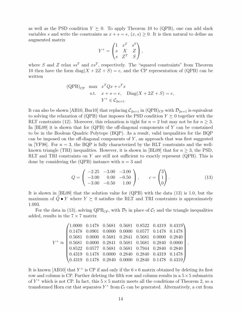
Figure 1: Gap to optimal value for Burer-Letchford QPB problem (n = 3)

Theorem 7 can be used. In either case imposing the new constraint and re-solving resultsin a new matrix Y + with lower objective value. The same 5 × 5 principal submatrix againfails to be CP, so another cut can be generated and the process repeated. In Figure 1 weshow the effect of executing this process using the cuts from Theorem 7, normalized usingI •V = 1. After adding 21 cuts, the gap to the true solution value of the problem is reducedbelow 10−8. (The rank condition in Theorem 2 fails after 3 cuts are added, but this has noeffect on the cuts from Theorem 7.)

Before continuing, we remark that there are other known approaches that obtain anoptimal value for the (QPB) instance (13) without branching. For example, in [AB10]it is shown that for n = 3, (QPB) can be exactly represented using DNN matrices viaa triangulation of the 3-cube. This representation provides a tractable formulation thatreturns the exact optimal solution value for the original problem. A completely differentapproach is based on using the result of Theorem 10 and writing a dual for (QPB)CP thatinvolves the cone C∗n+1. It then turns out that using the cone K1

7 as an inner approximationof C∗7 also obtains the exact solution value for the Burer-Letchford instance (13). It shouldbe noted, however, that both of these approaches involve “extended variable” formulationsof the problem, whereas the procedure based on adding cuts operates in the original problemspace.

Next we consider the problem of computing the maximum stable set in a graph. Let Abe the adjacency matrix of a graph G on n vertices, and let α be the maximum size of astable set in G. It is known [dKP02] that

α−1 = min{

(I + A) •X : eeT •X = 1, X ∈ Cn}. (14)

Relaxing Cn to Dn results in the Lovasz-Schrijver bound

(ϑ′)−1 = min{

(I + A) •X : eeT •X = 1, X ∈ Dn}. (15)

The bound ϑ′ was first established (via a different derivation) by Schrijver as a strengtheningof Lovasz’s ϑ number.

For our first example, with n = 12, let G12 be the complement of the graph correspondingto the vertices of a regular icosahedron [BdK02]. Then α = 3 and ϑ′ ≈ 3.24, a gap of

15

approximately 8%. A notable feature of the stable set problem for G12 is that using thecone K1

12 to approximate the dual of (14) provides no improvement over K012, corresponding

to the dual of (15) [BdK02]. For the solution matrix X from (15), the incidence matrix ofG(X) is

0 1 1 1 1 1 0 0 0 0 0 01 0 1 1 0 0 1 1 0 0 0 01 1 0 0 1 0 1 0 1 0 0 01 1 0 0 0 1 0 1 0 1 0 01 0 1 0 0 1 0 0 1 0 1 01 0 0 1 1 0 0 0 0 1 1 00 1 1 0 0 0 0 1 1 0 0 10 1 0 1 0 0 1 0 0 1 0 10 0 1 0 1 0 1 0 0 0 1 10 0 0 1 0 1 0 1 0 0 1 10 0 0 0 1 1 0 0 1 1 0 10 0 0 0 0 0 1 1 1 1 1 0

. (16)

It is then easy to see that there are many principal submatrices of the matrix X, upto size 9 × 9, that meet the conditions of Lemma 1. For example, consider the principalsubmatrix formed by omitting rows and columns {6, 8, 9}, partitioned into the sets I1 ={1, 2, 3, 10, 11, 12}, I2 = {4}, I3 = {5}, I4 = {7}. After a suitable permutation this 9 × 9matrix has the form (7), with n1 = 6, n2 = n3 = n4 = 1, and it is easy to see that G(X i)is a CP graph for i = 2, 3, 4. However, it turns out that matrices Aii satisfying the DNNfeasibility constraints of Lemma 1 exist, demonstrating that this principal submatrix is infact CP. This was the case for every principal submatrix satisfying the conditions of Lemma1 that we examined.

We next consider applying Lemma 2. It turns out that the vertices of G(X) can bepartitioned into 4 disjoint stable sets of size 3; one such partition uses the sets {1, 7, 10},{2, 6, 9}, {3, 8, 11} and {4, 5, 12}. Then Lemma 2 applies, and G(Xp) is a CP graph for eachp since each Xp is a 4 × 4 matrix. The DNN feasibility system in Lemma 2 does not havea solution, so Theorem 9 can be used to generate a cut separating X from C12. Adding thisone cut and re-solving, the gap to 1/α = 1

3is approximately 2× 10−8.

Before proceeding, it is worthwhile to note that for the stable set problem for G12, Lemma2 could actually be used to reformulate the problem (14) so that the exact solution valueα = 1/3 is obtained without adding any cuts. To see this, note that for problem (14) on agraph G with adjacency matrix A, it is obvious that xij = 1 =⇒ aij = 0, or in other wordsG(X) ⊂ G, where G is the complement of G. For the graph G12, the adjacency matrix forG is precisely that of G(X) in (16). Applying Lemma 2, the condition X ∈ C12 in (14) canbe replaced by an equivalent condition involving 81 matrices in D4, and the problem solvedexactly. Compared to the procedure of first solving a relaxation over D12 and then adding acut based on the solution G(X), the reformulation has the advantage that only one problemis solved. However, prior knowledge of the underlying problem structure is essential to thereformulation but is unused by the procedure based on adding cuts.

We next consider several stable set problems from [PVZ07]. These problems, of sizesn ∈ {8, 11, 14, 17}, are specifically constructed to be difficult for SDP-based relaxations suchas (15). We refer to the underlying graphs as G8, G11, G14 and G17. First consider G8, for

16

3 1

3.15

3.2

3.25

3.3

3.35

3.4

3.45

3.5

Boun

d for max stable set

3

3.05

3.1

3.15

3.2

3.25

3.3

3.35

3.4

3.45

3.5

0 20 40 60 80 100

Boun

d for max stable set

Iteration

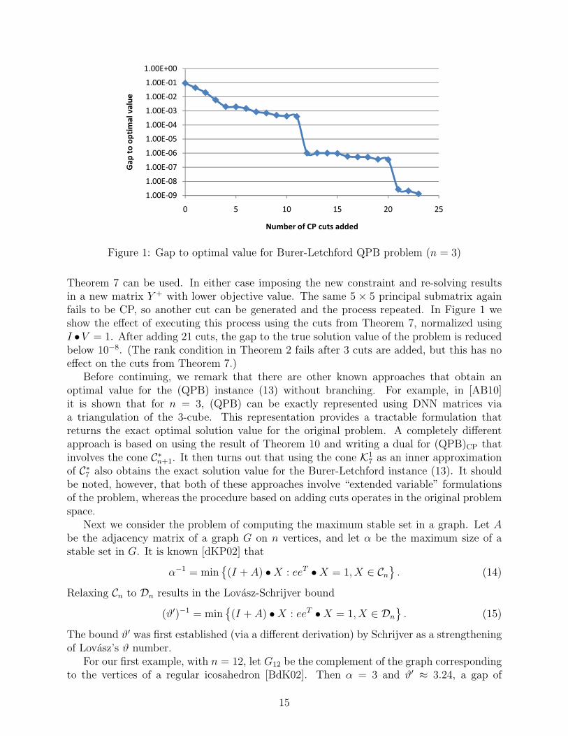
Figure 2: Bounds on max stable set for G8

which α = 3. The incidence matrix of G8 is

0 0 1 1 0 1 1 10 0 1 1 1 1 0 11 1 0 0 1 0 1 11 1 0 0 1 1 1 00 1 1 1 0 0 1 01 1 0 1 0 0 0 11 0 1 1 1 0 0 01 1 1 0 0 1 0 0

. (17)

It is clear that the vertices of G8 can be partitioned into 4 stable sets of size 2. Sincewe could assume that G(X) ∈ G8 (see the discussion above), Lemma 2 could be used toreformulate the problem (14), as described above, so that the exact value of α is obtained.Instead, we apply the methodology of first solving the problem (15), and obtain a solutionX = X0 ∈ D12 with G(X0) as in (17). For each partitioning of G(X0) into 4 stable sets ofsize 2 we generate a cut from Theorem 9, and the augmented problem is then re-solved toobtain a new solution X1. We then attempt to generate additional cuts based on G(X1),re-solve the problem to get a new solution X2, and continue. On iteration i we generateone cut for each partitioning of G(X i) into 4 stable sets of size 2. The resulting bounds onthe max stable set obtained for 100 iterations of this procedure are illustrated in Figure 2.The bound on α = 3 drops to approximately 3.078 on iteration 2, and then decreases slowlyon subsequent iterations. The number of cuts generated is 3 on iterations 0 and 1, 1 oniterations 2-30, and 3 or 4 per iteration thereafter. By comparison, in [BFL10] the gap toα for this problem is closed to zero, using copositivity cuts specialized for the max-cliqueproblem posed on the complement graph G8.

For the graphs Gn, n ∈ {11, 14, 17}, it is not possible to use Lemma 7 or Lemma 9 toexactly reformulate the condition X ∈ Cn in terms of DNN matrices. For these problems weused the following computational approach. We first solved (15) to obtain the solution X andthen found all possible structures consisting of 4 disjoint stable sets of size 2 in G(X). (The

17

0

1

2

3

4

5

6

7Fr

eque

ncy

n=11

n=14

n=170

1

2

3

4

5

6

7Fr

eque

ncy

Gap to max stable set

n=11

n=14

n=17

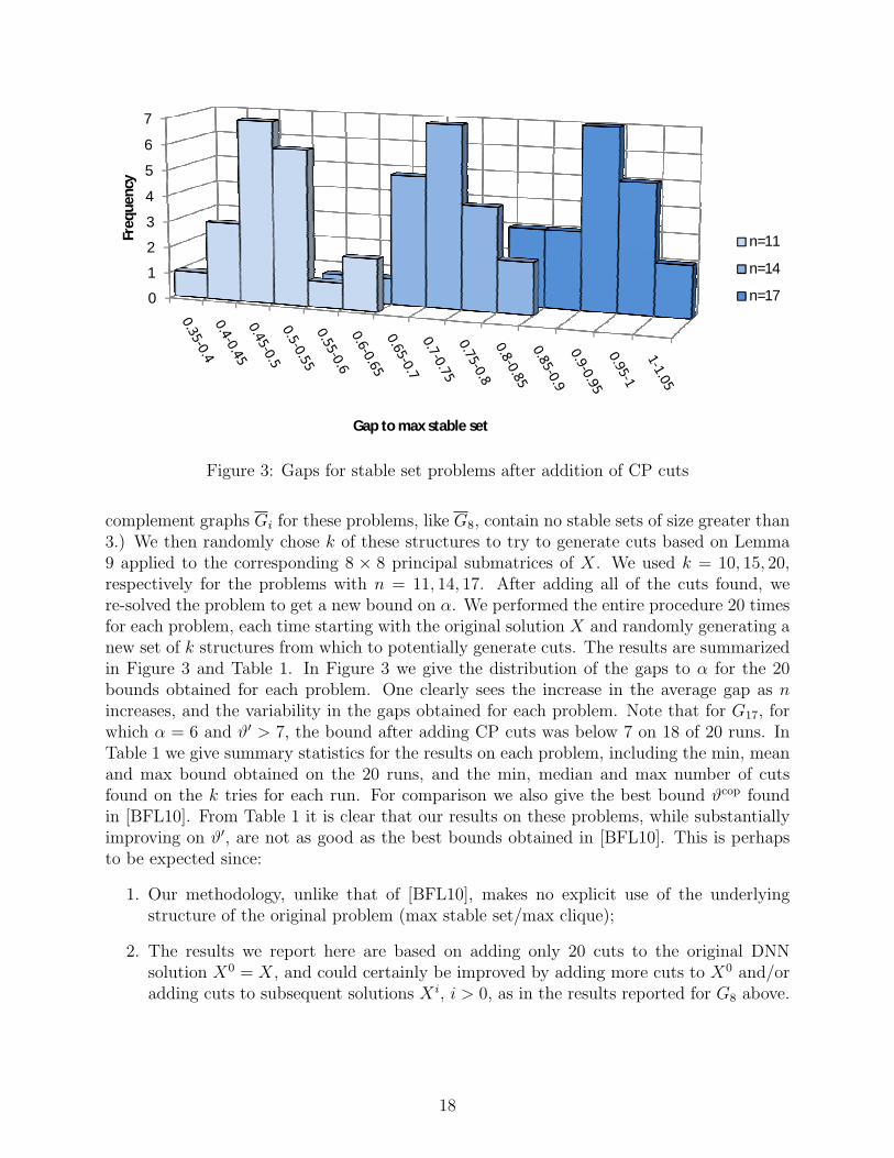
Figure 3: Gaps for stable set problems after addition of CP cuts

complement graphs Gi for these problems, like G8, contain no stable sets of size greater than3.) We then randomly chose k of these structures to try to generate cuts based on Lemma9 applied to the corresponding 8 × 8 principal submatrices of X. We used k = 10, 15, 20,respectively for the problems with n = 11, 14, 17. After adding all of the cuts found, were-solved the problem to get a new bound on α. We performed the entire procedure 20 timesfor each problem, each time starting with the original solution X and randomly generating anew set of k structures from which to potentially generate cuts. The results are summarizedin Figure 3 and Table 1. In Figure 3 we give the distribution of the gaps to α for the 20bounds obtained for each problem. One clearly sees the increase in the average gap as nincreases, and the variability in the gaps obtained for each problem. Note that for G17, forwhich α = 6 and ϑ′ > 7, the bound after adding CP cuts was below 7 on 18 of 20 runs. InTable 1 we give summary statistics for the results on each problem, including the min, meanand max bound obtained on the 20 runs, and the min, median and max number of cutsfound on the k tries for each run. For comparison we also give the best bound ϑcop foundin [BFL10]. From Table 1 it is clear that our results on these problems, while substantiallyimproving on ϑ′, are not as good as the best bounds obtained in [BFL10]. This is perhapsto be expected since:

1. Our methodology, unlike that of [BFL10], makes no explicit use of the underlyingstructure of the original problem (max stable set/max clique);

2. The results we report here are based on adding only 20 cuts to the original DNNsolution X0 = X, and could certainly be improved by adding more cuts to X0 and/oradding cuts to subsequent solutions X i, i > 0, as in the results reported for G8 above.

18

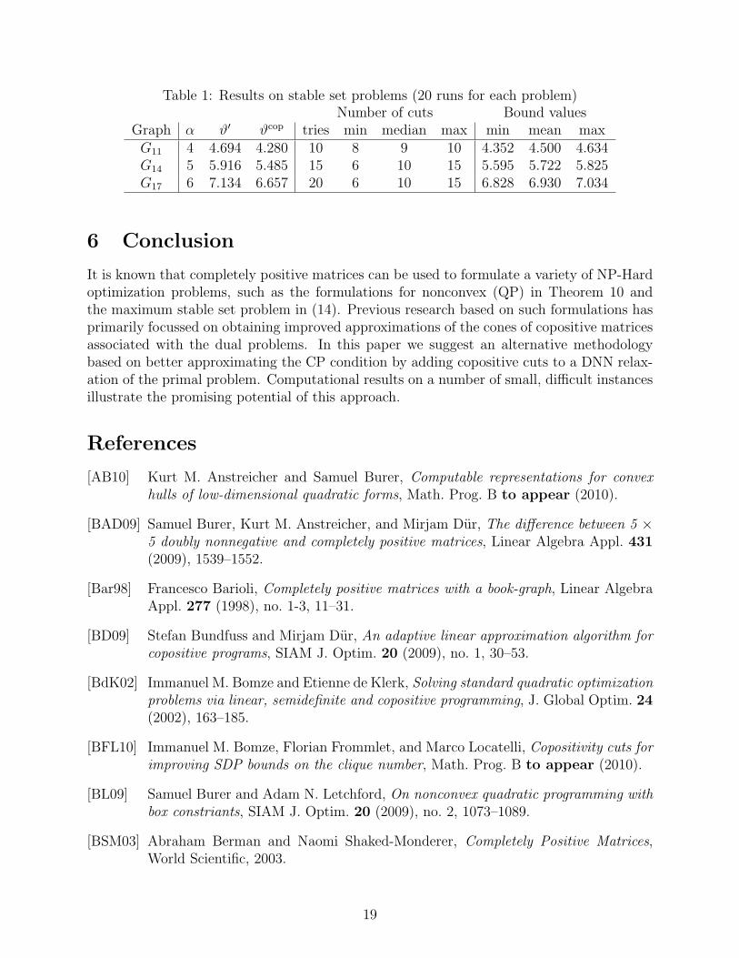
Table 1: Results on stable set problems (20 runs for each problem)Number of cuts Bound values

Graph α ϑ′ ϑcop tries min median max min mean maxG11 4 4.694 4.280 10 8 9 10 4.352 4.500 4.634G14 5 5.916 5.485 15 6 10 15 5.595 5.722 5.825G17 6 7.134 6.657 20 6 10 15 6.828 6.930 7.034

6 Conclusion

It is known that completely positive matrices can be used to formulate a variety of NP-Hardoptimization problems, such as the formulations for nonconvex (QP) in Theorem 10 andthe maximum stable set problem in (14). Previous research based on such formulations hasprimarily focussed on obtaining improved approximations of the cones of copositive matricesassociated with the dual problems. In this paper we suggest an alternative methodologybased on better approximating the CP condition by adding copositive cuts to a DNN relax-ation of the primal problem. Computational results on a number of small, difficult instancesillustrate the promising potential of this approach.

References

[AB10] Kurt M. Anstreicher and Samuel Burer, Computable representations for convexhulls of low-dimensional quadratic forms, Math. Prog. B to appear (2010).

[BAD09] Samuel Burer, Kurt M. Anstreicher, and Mirjam Dur, The difference between 5 ×5 doubly nonnegative and completely positive matrices, Linear Algebra Appl. 431(2009), 1539–1552.

[Bar98] Francesco Barioli, Completely positive matrices with a book-graph, Linear AlgebraAppl. 277 (1998), no. 1-3, 11–31.

[BD09] Stefan Bundfuss and Mirjam Dur, An adaptive linear approximation algorithm forcopositive programs, SIAM J. Optim. 20 (2009), no. 1, 30–53.

[BdK02] Immanuel M. Bomze and Etienne de Klerk, Solving standard quadratic optimizationproblems via linear, semidefinite and copositive programming, J. Global Optim. 24(2002), 163–185.

[BFL10] Immanuel M. Bomze, Florian Frommlet, and Marco Locatelli, Copositivity cuts forimproving SDP bounds on the clique number, Math. Prog. B to appear (2010).

[BL09] Samuel Burer and Adam N. Letchford, On nonconvex quadratic programming withbox constriants, SIAM J. Optim. 20 (2009), no. 2, 1073–1089.

[BSM03] Abraham Berman and Naomi Shaked-Monderer, Completely Positive Matrices,World Scientific, 2003.

19

[Bur09] Samuel Burer, On the copositive representation of binary and continuous nonconvexquadratic programs, Math. Prog. 120 (2009), no. 2, 479–495.

[Bur10] , Optimizing a polyhedral-semidefinite relaxation of completely positive pro-grams, Math. Prog. Comp. to appear (2010).

[BX04] Abraham Berman and Changqing Xu, 5 × 5 Completely positive matrices, LinearAlgebra Appl. 393 (2004), 55–71.

[DA09] Hongbo Dong and Kurt Anstreicher, On ‘5 × 5 Completely positive matrices’,Working paper, Dept. of Management Sciences, University of Iowa (2009).

[dKP02] Etienne de Klerk and Dmitrii V. Pasechnik, Approximation of the stability numberof a graph via copositive programming, SIAM J. Optim. 12 (2002), no. 4, 875–892.

[DS08] Mirjam Dur and Georg Still, Interior points of the completely positive cone, Elec-tron. J. Linear Algebra 17 (2008), 48–53.

[HJ67] Marshall Hall Jr., Combinatorial Theory, Blaisdell Publishing Company, 1967.

[HJR05] Leslie Hogben, Charles R. Johnson, and Robert Reams, The copositive completionproblem, Linear Algebra Appl. 408 (2005), 207–211.

[KB93] Natalia Kogan and Abraham Berman, Characterization of completely positivegraphs, Discrete Math. 114 (1993), 297–304.

[PVZ07] Javier Pena, Juan Vera, and Luis F. Zuluaga, Computing the stability number of agraph via linear and semidefinite programming, SIAM J. Optim. 18 (2007), no. 1,87–105.

[Stu99] Jos F. Sturm, Using SeDuMi 1.02, a MATLAB toolbox for optimization over sym-metric cones, Optim. Methods and Software 11-12 (1999), 625–653.

[Val89] Hannu Valiaho, Almost copositive matrices, Linear Algebra Appl. 116 (1989), 121–134.

[YF98] Yasutoshi Yajima and Tetsuya Fujie, A polyhedral approach for nonconvexquadratic programming problems with box constraints, J. Global Optim. 13 (1998),151–170.

20