Nonlinear disturbance observersDesign and applications to Euler-Lagrange systems

Alireza Mohammadi, Horacio J. Marquez, and Mahdi Tavakoli

POC: H. J. Marquez (hmarquez@ualberta.ca)

August 26, 2016

Estimation of unknown inputs and/or disturbances has been a topic of constant interestin the control engineering for the past several decades. The reader is referred to [1] for a2

detailed survey on the development of unknown input observers. Disturbance observers (DOB)are a special class of unknown input observers that were introduced for robust motion control4

applications in the early 1980s [2]. Since their introduction in the literature, DOBs have beenemployed efficaciously in numerous robust control and fault detection applications ranging from6

process control [3], [4] to mechatronics [5], [6], [7], [8], [9]. Figure 1 depicts a DOB that isemployed in a typical control system. As can be seen in the figure, the DOB is used to reconstruct8

unknown disturbances that are acting on the plant from the measured output variables and theknown control inputs applied to the system. The output of the DOB, namely, the estimated10

disturbance, can then be used in feedforward compensation of disturbances or faults.

Disturbance observers possess several promising features in control applications [10].12

The most important feature is the add-on or “patch” feature. The disturbance feedforwardcompensation can be employed as an add-on to a previously designed feedback control. Indeed,14

there is no need to change the existing control laws, which might have been extensively used andestablished in their respective literatures, such as PID feedback control used in industrial systems,16

model predictive control used in process systems, and gain scheduling feedback control used inflight control. In order to improve the disturbance rejection and robustness abilities, DOB-based18

compensation can be augmented with the baseline feedback control designed using conventionaltechniques. This feature has made using DOBs an appealing approach for rejecting disturbances20

in commercial control applications. See [11] for a discussion on commercialization aspects ofDOBs.22

In general, DOB design has been carried out using linear system techniques [12], [13],[5], [14], [15], [16], [17], [18], [19]. In order to overcome the limitations of linear disturbance24

observers (LDOB) in the presence of highly nonlinear and coupled dynamics, researchershave started investigating nonlinear disturbance observers (NDOB) for systems with nonlinear26

1

This paper appears in IEEE Control Systems Magazine, 2017. DOI: 10.1109/MCS.2017.2696760

TABLE 1: An overview of nonlinear disturbance observer (NDOB) classes: Based on their underlying dynamicalequations and similarity to state observers, NDOBs can be categorized into two classes; namely, basic NDOBs andsliding mode-based NDOBs.

NDOB class References Applications

Basic[20], [27], [28][29], [30], [31]

mechatronics, robotics,and teleoperation

Sliding mode-like[32], [33], [34]

[35], [36]robust fault detection,

attitude and formation control in aerospace applications

dynamics during the past decade [20], [21], [22], [23], [24]. A line of research has alsobeen initiated to address some of the more theoretical questions that arise in the context of2

NDOBs [23], [25], [26] where singular perturbation and time-scale separation analyses have beenemployed. The papers [23], [25], [26] have also extensively studied the problem of recovering4

nominal transient performance in the presence of disturbances using NDOBs. There exist varioustypes of NDOBs proposed in the literature and each of them is suitable for a specific set of6

applications. A possible way to categorize NDOBs is to consider their underlying dynamicalequations to state observers. Based on this criterion, NDOBs can be categorized into two general8

classes; namely, basic NDOBs and sliding mode-based NDOBs. Basic NDOBs are extensivelyused in mechatronics and robotics applications and are the generalization of the famous linear10

DOB in [12], [5] to the context of systems with nonlinear dynamics. Sliding mode-like NDOBsare appealing in applications where disturbance estimation error needs to converge in finite12

time such as fault-detection applications. Presence of discontinuities in the sliding mode-basedNDOBs, which may give rise to the chattering phenomenon, make their analysis harder. Table 114

gives an overview of the existing NDOBs and their applications.

One of the restrictions of disturbance observers is that they require measurement of the16

states of the dynamical control system under study. A relatively new research direction in theDOB framework is to combine state and disturbance observers in the so-called generalized18

extended state observer framework which is essentially an output-based disturbance observer(see [37], [38] for further details).20

One of the most prominent applications of NDOBs is in the field of robotics. Varioustypes of disturbances such as joint frictions, unknown payloads, and varying contact points might22

adversely affect the stability and performance of the robotic control systems. By exploiting thespecial structure of dynamical equations of robotic systems, NDOB design takes a special form.24

A general NDOB gain design method for serial robotic manipulators, which builds upon the

2

work in [39], [21], has been recently proposed in the literature [29], [40]. The proposed NDOBgain can accommodate conventional LDOB/NDOB gains that were previously proposed in the2

literature [5], [39] and remove the previously existing restrictions on the types of joints, themanipulator configuration, or the number of degrees-of-freedom (DOFs). Since its introduction,4

this design method has been applied to other class of robotic systems such as observer-basedcontrol of 6-DOF parallel manipulators [30], improving transparency in virtual coupling for haptic6

interaction during contact tasks [31], and dynamic surface control of mobile wheeled invertedpendulums [41]. This serves as the motivation to investigate whether the NDOB structure in [29]8

can be applied to the more general class of Euler-Lagrange (EL) systems. Euler-Lagrange modelscan be effectively used to describe a plethora of physical systems ranging from mechanical and10

electromechanical to power electronic and power network systems [42], [43], [44], [45]. In thisarticle, the focus of applications is on robotic systems possessing EL dynamics.12

One of the latest applications of DOBs has been in the field of teleoperation where thereis a need for stability and transparency [46], [47], [48], [49], [16], [50]. Teleoperation involves14

indirect performance of a task in a remote environment and is used to extend a person’s sensingand manipulation capability to a remote location [51]. Every teleoperation system consists of a16

master robot (user interface) and a slave robot, which exchange different types of informationsuch as force, position, and visual and auditory data via a communication channel (see Figure 2).18

The master interacts with the human operator and the slave interacts with the remote environment.The human operator applies position commands to the master robot. The slave robot responds20

to the received position commands from the communication channel and moves to the desiredposition in the remote environment. If force feedback from the slave side to the master side is22

present, the system is called a bilateral teleoperation system to distinguish it from a unilateralteleoperation system, in which no force is reflected to the user. A bilateral teleoperation system24

is said to be transparent if the slave robot follows the position of the master robot and themaster robot faithfully displays the slave-environment contact force to the human operator.26

Major challenges encountered in control of teleoperation systems include nonlinearities anduncertainties, communication delays, and unknown disturbances.28

Uncertainties, nonlinearities, and possible time delays in the communication channelconstitute the “must solve” problem, given that they can compromise system stability, which30

must be guaranteed at any cost. A secondary problem, which is also of critical importance, isdisturbance rejection. Indeed, rejecting the effect of unknown disturbances is critical given that32

robust performance and stability largely depends on being able to do so. A promising approachto suppressing such disturbances is to make use of NDOBs.34

In this article, NDOB design and its applications to Euler-Lagrange and teleoperation

3

systems are presented. First, the earliest variant of LDOBs, proposed in [2] (see also [12]) andwhich has inspired the research on DOBs, is briefly described to motivate further the development2

of its nonlinear counterpart. Next, the structure of an NDOB proposed in [21] (see also [10], [11]),that has a basic structure and can be effectively employed in EL and teleoperation systems, is4

presented. Some properties of this class of NDOBs such as semi/quasi-passivity property, whichhave not been discussed in the previous NDOB literature, are presented in this article.6

We then turn to EL systems and present the general observer design method, which isbased on the NDOB structure in [39], [21], for this class of dynamical systems. We show that8

the NDOB structure in [29], which was first proposed for serial robotic manipulators, can beused for the more general class of EL systems. Moreover, we show how the proposed NDOB10

can be used along with well-established control schemes such as passivity-based control.

As an important application, NDOBs are incorporated into the framework of the 4-12

channel teleoperation architecture. This control architecture is used extensively to achieve fulltransparency in the absence of time delays [52], [53], [54]. Unfortunately, it is well known14

that unless disturbances are explicitly accounted for during the design, their presence maycause poor position/force tracking or even instability of the 4-channel teleoperation system. The16

proposed NDOB enables the 4-channel teleoperation architecture to achieve full transparency andexponential disturbance and position tracking under slow-varying disturbances. In the case of fast-18

varying disturbances, the proposed NDOBs guarantee global uniform ultimate boundedness of thetracking errors. In this article, it is demonstrated how the proposed NDOB can be accommodated20

in the 4-channel bilateral teleoperation architecture to guarantee stability and transparency of theteleoperation system in the presence of disturbances and in the absence of communication delays.22

Throughout the rest of the article we will employ the following notation:

Notation. We let R, R+, and R+0 denote the field of real numbers, and the sets of positive24

and nonnegative real numbers, respectively. Rn represents the set of n-dimensional vectors withreal components. The maximum and the minimum eigenvalues of a square matrix are represented26

by λmax(.) and λmin(.), respectively. Euclidean norm and induced matrix 2-norm are used to definevector and matrix norms. In other words, |x| =

√xTx represents the vector norm for a given28

vector x ∈ Rn. Likewise,∣∣X∣∣ =

√λmax(XTX) for a given matrix X ∈ Rn×n. Given two square

matrices A, B ∈ Rn×n, the inequality A ≥ B means that A − B is a positive semi-definite30

matrix.

4

Linear Disturbance Observer

Since the focus of this article is on NDOBs, only the first variant of LDOBs will be briefly2

presented. This DOB was first proposed in [2], [12] for robust motion control systems and hassince motivated much research in the control community. Rigorous analyses and definitions will4

be presented in the context of NDOBs in the next section. For a detailed discussion on othervariants of LDOBs, the reader is referred to [1], [10], [55], [11] and references therein.6

Figure 3 demonstrates the block diagram of a DOB-based robust motion control systemproposed in [2], [12]. The torque τ represents the control input is represented. Moreover, the8

parameters J and Ld represent mass/inertia and gain of the DOB, which is a design parameter,respectively. The unknown disturbance τd lumps the effect of disturbances such as harmonics10

and friction; namely,

τd = τd,f + τd,h,

where τd,f and τd,h are the friction and harmonic disturbances, respectively. Similarly, other12

disturbances can be incorporated in the lumped disturbance τd.

The role of the DOB in Figure 3 is to estimate the lumped disturbance torque τd from the14

state θ and input torque τ . The equation of motion is given by

Jθ = τ + τd − τd.

Feeding forward the disturbance estimate τd suppresses the adverse effect of τd on the motion16

control system in Figure 3. In the ideal case, when τd = τd, the lumped disturbance will becanceled out and the control input τ acts on the nominal control system with no disturbances.18

As it can be seen from the block diagram in Figure 3

τd = − Ld

s+ Ld

(JLdθ + τ − τd

)+ JLdθ =

Ld

s+ Ld(Jsθ + τ − τd).

Therefore, the disturbance estimate satisfies20

τd =Ld

s+ Ldτd =

11Lds+ 1

τd.

5

If the lumped disturbance term τd remains within the bandwidth of the DOB, it can be accuratelyestimated by the output of the DOB, namely, τd. Indeed, larger DOB gains give rise to better2

transient responses in estimation. The nonlinear counterpart of this property of DOBs is shownin the next sections.4

Nonlinear Disturbance Observer

In this section, the general NDOB structure of [21] and some of its properties that have not6

been discussed in the previous NDOB literature are presented. In particular, semi/quasi-passivityand uniform ultimate boundedness (see “Brief Review of Nonlinear Systems” for the definition8

of these two concepts) of this class of NDOBs are discussed in this section. The NDOB gaindesign for EL systems will be presented in the next section.10

Nonlinear disturbance observer structure and assumptions on disturbances

Consider the following nonlinear control affine system12

x = f(x) + g1(x)u+ g2(x)d,

y = h(x), (1)

where x ∈ Rn is the state vector, u ∈ Rm is the control input vector, d ∈ Rl is the lumpeddisturbance vector, and y ∈ Rm is the output vector. The lumped disturbance vector d is assumed14

to lump the effect of unknown disturbances. The functions f , g1, and g2 in (1) are assumed tobe smooth. Additionally, the functions f and g1 represent the nominal model of the system.16

The problem to solve is to design an observer, called the disturbance observer, to estimatethe lumped disturbance vector d from the state and input vectors. The output of the DOB can18

be used in feedforward compensation of disturbances.

An NDOB structure, proposed in [21] (see also [10], [11]), that can be employed to estimate20

the lumped disturbance vector d is

z = −Ld(x)g2(x)z − Ld(x)[f(x) + g1(x)u+ g2(x)p(x)

],

d = z + p(x), (2)

where z ∈ Rl is the internal state vector of the DOB, d ∈ Rl is the estimated disturbance22

6

vector, and p(x) is called the auxiliary vector of the NDOB. Finally, the matrix Ld(x) is calledthe NDOB gain matrix. As it will be shown in this section, there should exist a certain relation2

between the auxiliary vector p(x) and the NDOB gain Ld(x). Figure 4 depicts the block diagramof the NDOB-based robust control system proposed in [21]. The disturbance tracking error is4

defined to be

ed := d− d. (3)

Before presenting the disturbance tracking error dynamics of the NDOB (2), we provide6

a brief sketch of how this NDOB is derived. Taking the derivative of (3) and assuming d ≈ 0

yields8

ed =˙d.

We would like the estimation error to asymptotically converge to zero. Therefore, it is desirableto have10

ed =˙d = −Led,

where L = αdI and αd is some positive scalar. By (3), we have

˙d = −L(d− d

).

Assuming that g2(x) ∈ Rn×l has full column rank for all x, we define the following gain matrix12

Ld(x) := αdg†2(x), (4)

where g†2(x) is a left inverse of g2(x), e.g., g†2(x) =(gT2 (x)g2(x)

)−1gT2 (x). Then, Ld(x)g2(x) = L.

Hence, from (1), we have14

˙d = −L(d− d

)= −Ld(x)g2(x)d+ Ld(x)g2(x)d︸ ︷︷ ︸

Ld(x)(x−f(x)−g1(x)u

) .Accordingly,

˙d = −Ld(x)g2(x)d+ Ld(x)x− Ld(x)

(f(x) + g1(x)u

).

Before proceeding further, we remark that if the derivative of the state x is assumed to be16

available, then design is completed at this stage. This is the case for the 4-channel controlarchitecture used in teleoperation systems where there are accelerometers available. This is further18

discussed later in the article. Defining the variable z := d − p(x) and inserting in the aboveequation, we get20

z + p(x) = −Ld(x)g2(x)z + Ld(x)g2(x)p(x) + Ld(x)x− Ld(x)(f(x) + g1(x)u

).

7

Therefore, if the relation

Ld(x) =∂p

∂x(x), (5)

holds between the NDOB gain matrix Ld(x) and the auxiliary vector p(x), then2

p(x) = Ld(x)x,

and we get the given expression for the NDOB given by (2).

Taking the derivative of (3), the tracking error dynamics can be computed as follows4

ed =˙d− d =︸︷︷︸

(2)

z + p(x)− d = −Ld(x)g2(x)z − Ld(x)[f(x) + g1(x)u︸ ︷︷ ︸

x−g2(x)d

+g2(x)p(x)]

+ p(x)− d

= −Ld(x)g2(x)z − Ld(x)[x+ g2(x)(p(x)︸︷︷︸

d−z

−d)]

+ p(x)− d

= −Ld(x)g2(x)z − Ld(x)[x+ g2(x)ed − g2(x)z

]+ p(x)− d

= −Ld(x)g2(x)ed − Ld(x)x+ p(x)− d.

Using (5) in the above expression, it can be seen that the disturbance tracking error dynamicsare governed by6

ed = −Ld(x)g2(x)ed − d. (6)

It is assumed that the observer gain Ld(x) has been designed to satisfy

−eTd Ld(x)g2(x)ed ≤ −αd|ed|2, (7)

uniformly with respect to x for some positive constant αd. In general, design of the NDOB8

gain matrix Ld(x) is not trivial. As it can be seen from Equation (7), one needs to know thestructure of g2(x) in order to design the gain matrix Ld(x). Therefore, determining this gain10

depends on the application under study. In the case of Euler-Lagrange systems and due to thespecial structure of the underlying dynamical equations, we are able to find such a gain matrix.12

Under the assumption that g2(x) has full row rank for all x, which is also the case for Euler-Lagrange systems under study in this article, an expression for Ld(x) is given in (??). The issue14

of designing Ld(x) for EL systems will be discussed in the next section. In order to analyze how

8

the NDOB in (2) achieves disturbance tracking, the Lyapunov candidate function Vd = 12eTd ed is

considered. Taking the derivative of Vd along the trajectories of (6) yields2

Vd = −eTd Ld(x)g2(x)ed − eTd d. (8)

Some prior knowledge regarding the lumped disturbance dynamics is required in order toanalyze further the performance of an NDOB in terms of stability and disturbance tracking. In4

this article, it is assumed that there exists a positive real constant ω such that

|d(t)| ≤ ω, for all t ≥ 0. (9)

We remark that the constant ω needs not be known precisely. The NDOB stability analysis only6

requires knowing some upper bounds on ω. The interested reader is referred to [19], [11] for adetailed discussion on estimating higher order disturbances in time series expansion, and to [21]8

in the case that the disturbances are generated by linear exosystems with known dynamics. Notealso that assumption (9) does not require knowing any special form for the lumped disturbance.10

Indeed, the ability to estimate unknown disturbances without the need for knowing their specialform has been one of the key motivations behind DOB research [5].12

Finally, we assume that the disturbance d satisfies the matching condition; namely, thereexists a smooth function gd(x) such that14

g1(x)gd(x) = g2(x), (10)

where |gd(x)| ≤ gd holds uniformly with respect to x for some positive constant gd. In otherwords, the lumped disturbance d and the control input u act on the system through the same16

channel. This matching condition serves the application purpose of this article. The interestedreader is referred to [24], [38] where progress has been made in order to relax this condition18

by using tools from geometric nonlinear control. Finally, we assume that |g2(x)| ≤ g2 holdsuniformly with respect to x for some positive constant g2.20

In order to investigate the add-on feature of NDOBs, the following DOB-based controlinput is considered22

9

u = un − βdy − gd(x)d, (11)

where βd is some non-negative constant, y is the vector of outputs, d is the estimated disturbanceprovided by the NDOB in (2), and the nominal control input un is designed for the system without2

disturbances, namely, the nominal control system

x = f(x) + g1(x)u,

y = h(x). (12)

The role of the feedforward term −gd(x)d in (11) is to suppress the adverse effects of4

unknown disturbances acting on the closed-loop system. The nominal closed-loop system vectorfield is denoted by6

f cl(x) = f(x) + g1(x)un. (13)

Under the matching condition and using the DOB-based control input (11) in (1), it can be seenthat8

x = f(x) + g1(x)(un − gd(x)ed − βdy

),

y = h(x). (14)

Semi/Quasi-passivity of NDOBs

In this section, we show that under the assumption of passivity (see “Brief Review of10

Nonlinear Systems” for the definition of passivity) of the nominal nonlinear system (12), theNDOB (2) is able to make the augmented nonlinear system and the NDOB semi/quasi-passive.12

This observation regarding the semi/quasi-passivity of the NDOB in [21] has not been reportedin the previous NDOB literature. Using (7) and (8) along with (9), it can be seen that14

Vd ≤ −αd|ed|2 + ω|ed|. (15)

10

The first thing to notice in Inequality (15) is that it immediately follows from the uniformultimate boundedness theorem (see “Brief Review of Nonlinear Systems”) that for all ed(0) ∈ Rl,2

the disturbance tracking error converges with an exponential rate, proportional to αd, to a ballcentered at the origin with a radius proportional to 1

αd. Since the ultimate bound and convergence4

rate of the NDOB (2) can be changed by tuning the design parameter αd, it is said to bepractically stable. Indeed, increasing the parameter αd results in better disturbance tracking6

response; that is, both convergence rate and accuracy of the disturbance observer are improvedwhen αd is increased. Note also that when the disturbance is generated by an exogenous system8

and Inequality (7) holds uniformly with respect to x, the uniform ultimate boundedness ofNDOB (2) holds irrespective of the closed-loop dynamics of the nonlinear system (1). It is10

noteworthy that the NDOB error dynamics, under the assumption of bounded disturbances, arebounded-input bounded-output (BIBO) stable (the reader is referred to [56] for further details).12

Finally, it is remarked that when ω = 0 the disturbance tracking error ed will converge to zeroasymptotically with an exponential rate.14

In order to analyze the semi/quasi-passivity property of the nonlinear system (1) alongwith (2) in the presence of disturbances, the candidate Lyapunov function V (x, ed) = Vn(x) +16

Vd(ed) is considered, where Vn is the candidate Lyapunov function for the nominal control systemx = f(x)+g1(x)u, with output y = h(x), for which the inequality Vn(x, u) ≤ yTu holds. Taking18

the derivative of V and using (14) along with Inequality (15) yields

V = Vn + Vd ≤ yT(un − gd(x)ed − βdy

)− αd|ed|2 + ω|ed|. (16)

In order to proceed further, Young’s Inequality is used; whereby, aT b ≤ |a|22ε

+ ε|b|22

for all vectors20

a, b ∈ RN and any arbitrary positive constant ε. It can be seen that

V ≤ yTun −(βd −

ε

2

)|y|2 −

[(αd −

ω + gd

2ε

)|ed|2 −

ωε

2

]︸ ︷︷ ︸H(ed)

, (17)

for some positive constant ε. Therefore, when22

βd ≥ε

2,

αd ≥ω + gd

2ε, (18)

11

the augmented nonlinear system (1) with NDOB (2) is a semi/quasi-passive system (see “BriefReview of Nonlinear Systems”) with input τn, output y, and H(ed) = (αd − ω+gd

2ε

)|ed|2 − ωε

2. In2

a similar way, it can also be shown that if the nonlinear system (1) is semi/quasi-passive, theaugmented nonlinear system with the NDOB (2) is semi/quasi-passive.4

Semi/quasi-passive systems have several appealing properties (see “Brief Review ofNonlinear Systems”). For instance, it can be shown that an output feedback of the form un = ξ(y)6

such that yT ξ(y) ≤ 0 makes the solutions of the semi-passive system ultimately bounded. It is tobe remarked that the semi/quasi-passivity of the augmented nonlinear system (1) with NDOB (2)8

is a direct result of feeding forward the disturbance estimate provided by the disturbance observer.

According to the inequalities in (18), the damping injection coefficient βd, can be chosen10

to be as small as desired, namely, by choosing the constant ε to be arbitrarily small, providedthat the coefficient αd, namely, the convergence rate of disturbance tracking error, is chosen12

to be sufficiently large. However, there exists a trade-off between the NDOB gain and noiseamplification. The reader is referred to [11], [29] for a discussion of choosing an optimal NDOB14

gain when measurement noise is present.

In this section, the add-on feature of NDOB (2) in companion with exponentially stabilizing16

nominal control laws is investigated. One of the applications of the presented material in thissection is in robotic systems that are controlled by computed-torque/feedback linearizing control18

laws (see the Section “Properties of augmented EL systems with NDOBs controlled by computed-torque/feedback linearizing schemes”). We assume that the control input un = un(x, t) makes20

the origin of the nominal closed-loop system globally exponentially stable and f(0) = 0.

When the control input un(x, t) makes the origin of the nominal closed-loop system x =22

f cl(x, t), where f cl(x, t) = f(x) + g1(x)un(x, t), globally exponentially stable and f(0) = 0,according to the converse Lyapunov function theorem (see “Brief Review of Nonlinear Systems”),24

there exists a function Vn(x, t) that satisfies

c1|x|2 ≤ Vn(x, t) ≤ c2|x|2,∂Vn

∂xf cl(x, t) +

∂Vn

∂t≤ −c3|x|2,∣∣∣∣∂Vn

∂x

∣∣∣∣ ≤ c4|x|, (19)

for some positive constants c1, c2, c3, and c4. Also, as it is shown in the proof of Theorem 4.1426

in [57], the inequality |f cl(x, t)| ≤ L|x| holds for some positive constant L and all x ∈ Rn.

12

In order to analyze the convergence properties of NDOB error dynamics together withthe exponentially stabilizing nominal control input un(x, t), the candidate Lyapunov function2

V (x, ed, t) = Vn(x, t) + Vd(ed) is considered. It can be seen from (19) that c1|x|2 + 12|ed|2 ≤

V (x, ed, t) ≤ c2|x|2 + 12|ed|2. Taking the derivative of V yields the following inequality4

V ≤ −αd|ed|2 − c3|x|2 + ω|ed|. (20)

Using Young’s inequality, it can be seen that

V ≤ −cd|ed|2 − cx|x|2 + ω0. (21)

where cd = αd − ω2ε

, cx = c3, ω0 = ε2ω, and ε is an arbitrary positive constant.6

The design parameters αd and ε should be chosen such that cd, cx ∈ R+. It follows fromthe uniform ultimate boundedness theorems (see “Brief Review of Nonlinear Systems”) that for8

all x(0) ∈ Rn and all ed(0) ∈ Rl, the disturbance tracking error ed and the state x converge withan exponential rate, proportional to mincd, cx, to a ball centered at the origin with a radius10

proportional to 1mincd,cx .

12

Comparison with linear DOBs in state-space form

Let the state-space description of a linear system be given by14

x = Ax+Buu+Bdd,

y = Cx.

Then as it is stated in [10] the dynamical equations of the NDOB (2) reduces to

z = −LdBd(z + Lx)− Ld(Ax+Buu),

d = z + Ldx,

which coincides with the traditional unknown input observers under certain assumptions16

(see [11]). It can be shown that choosing the constant gain matrix Ld such that −LdBd is Hurwitzguarantees BIBO stability of the disturbance tracking error. Moreover, when the disturbances18

are constant, asymptotic convergence of the disturbance tracking error is achieved (see [10] forfurther details).20

13

Nonlinear Disturbance Observer Design for Euler-Lagrange Systems

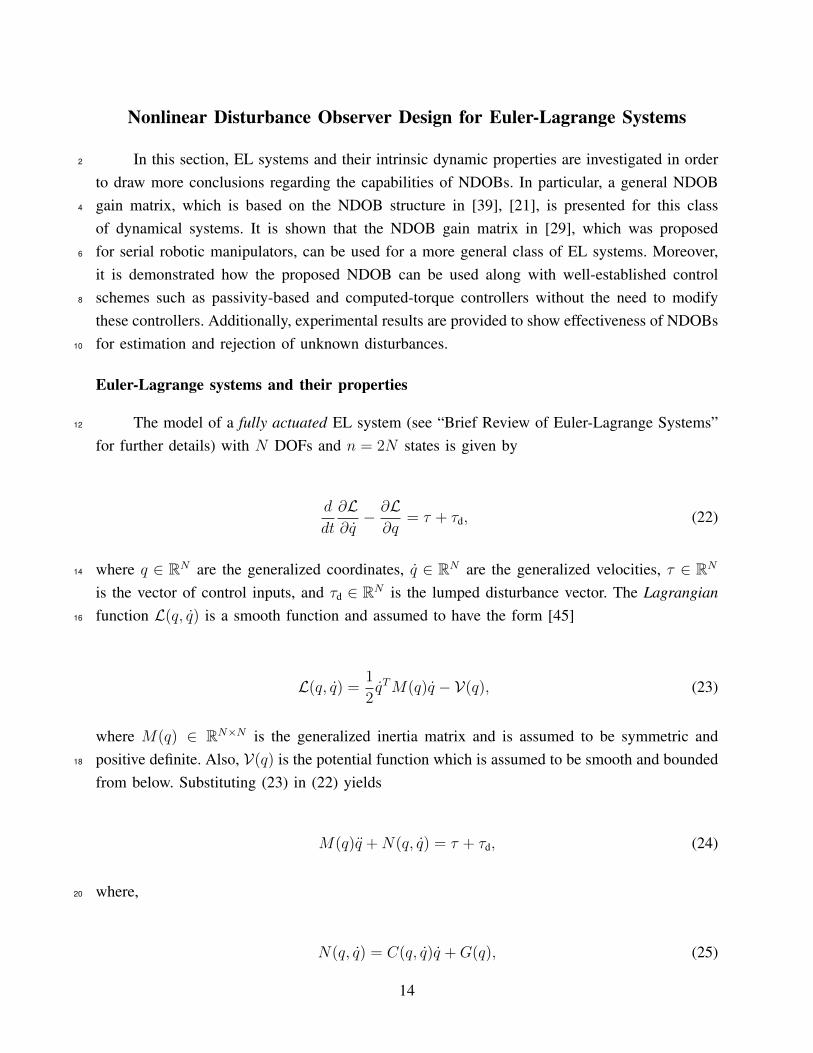
In this section, EL systems and their intrinsic dynamic properties are investigated in order2

to draw more conclusions regarding the capabilities of NDOBs. In particular, a general NDOBgain matrix, which is based on the NDOB structure in [39], [21], is presented for this class4

of dynamical systems. It is shown that the NDOB gain matrix in [29], which was proposedfor serial robotic manipulators, can be used for a more general class of EL systems. Moreover,6

it is demonstrated how the proposed NDOB can be used along with well-established controlschemes such as passivity-based and computed-torque controllers without the need to modify8

these controllers. Additionally, experimental results are provided to show effectiveness of NDOBsfor estimation and rejection of unknown disturbances.10

Euler-Lagrange systems and their properties

The model of a fully actuated EL system (see “Brief Review of Euler-Lagrange Systems”12

for further details) with N DOFs and n = 2N states is given by

d

dt

∂L∂q− ∂L∂q

= τ + τd, (22)

where q ∈ RN are the generalized coordinates, q ∈ RN are the generalized velocities, τ ∈ RN14

is the vector of control inputs, and τd ∈ RN is the lumped disturbance vector. The Lagrangianfunction L(q, q) is a smooth function and assumed to have the form [45]16

L(q, q) =1

2qTM(q)q − V(q), (23)

where M(q) ∈ RN×N is the generalized inertia matrix and is assumed to be symmetric andpositive definite. Also, V(q) is the potential function which is assumed to be smooth and bounded18

from below. Substituting (23) in (22) yields

M(q)q +N(q, q) = τ + τd, (24)

where,20

N(q, q) = C(q, q)q +G(q), (25)

14

and C(q, q)q ∈ RN is the vector of Coriolis and centrifugal forces. Also, G(q) := ∂V∂q

are theforces generated by potential fields such as the gravitational field. As is customary in the robotics2

literature, the vector G(q) is called the gravity vector in this article.

Following the EL systems literature (see, for example, [58]), it is assumed that the EL4

model under study has the following properties:

P16

1) The inertia matrix M(q) satisfies

ν1I ≤M(q) ≤ ν2I, (26)

where ν1 and ν2 are some positive constants and Inequality (26) holds uniformly with8

respect to q.2) The matrix M(q) − 2C(q, q) is skew-symmetric; namely, zT

[M(q) − 2C(q, q)

]z = 0 for10

all z ∈ RN .3) The matrix C(q, q) is bounded in q and linear in q; namely,12

C(q, q)z = C(q, z)q, (27)∣∣C(q, q)∣∣ ≤ kc|q|, (28)

for all z ∈ RN and some positive constant kc.4) Let qr ∈ Rn be an arbitrary vector. There exists a linear parameterization for EL models14

of the form M(q)qr +C(q, q)qr +G(q) = Υ(q, q, qr, qr)θ, where Υ is a regressor matrix ofknown functions and θ is a vector containing EL system parameters.16

It is remarked that the EL dynamics (24) can be written in the nonlinear control affineform (1) with18

x =

[q

q

]∈ Rn,

f(x) =

[q

M−1(q)−C(q, q)q −G(q)

],

g1(x) = g2(x) =

[0

M−1(q)

], (29)

where n = 2N is the dimension of the state space.

15

NDOB structure for EL systems

The lumped disturbance vector τd = τd(t) in (22) is assumed to satisfy |τd| ≤ ω for2

all t ≥ 0, for some positive constant ω. This class of disturbances includes but is not limited toharmonics and external disturbances.4

In EL systems, the NDOB dynamic equations in (2) take the form

z = −Ld(q, q)z + Ld(q, q)N(q, q)− τ − p(q, q),

τd = z + p(q, q). (30)

This NDOB was first proposed in [39]; however, no general structure for the observer gain6

matrix Ld(q, q) was given in that work. Defining the disturbance tracking error to be

∆τd := τd − τd,

its governing dynamics can be computed as follows8

∆τd = ˙τd − τd =︸︷︷︸(30)

z + p− τd = −Ld(.)z + Ld(.)[N(.)− τ︸ ︷︷ ︸−M(q)q+τd

−p(.)]

+ p(.)− τd =

−Ld(.)(τd − p) + Ld(.)[−M(q)q + τd − p(.)

]+ p(.)− τd = −Ld(.)∆τd + p(.)

−Ld(.)M(q)q − τd

In order to remove dependence of the disturbance tracking error dynamics on acceleration vectorq, the relation10

d

dtp(q, q) = Ld(q, q)M(q)q.

should hold. On the other hand, p(q, q) = ∂p∂qq + ∂p

∂qq. Therefore, ∂p

∂q= 0 and p(.) is a function

of q. Also, the relation12

∂p

∂q= Ld(q, q)M(q),

16

should hold between the NDOB gain and auxiliary vector. Since p(.) is a function of q, itnecessarily follows that2

Ld(q, q) = A(q)M−1(q), (31)

where ∂p∂q

= A(q). Therefore, as in [29], the following form may be used for the gain matrix:

Ld(q) = X−1M−1(q), (32)

where X is a constant symmetric and positive definite N × N matrix to be determined. For4

simplicity of exposition, the matrix X is considered to be equal to α−1I , where α = αdν2 andν2 is the positive constant in Property P1 of EL systems. Using the gain (32), it is seen that6

p(q) = X−1q. (33)

∆τd = −Ld(q)∆τd + τd, (34)

The following inequality, which is a special case of (7), immediately follows from PropertyP1 of EL systems and the NDOB gain matrix structure (32), with X = α−1I ,8

−∆τTd Ld(q)∆τd ≤ −αd|∆τd|2, for all q ∈ RN , ∆τd ∈ RN . (35)

Augmented dynamics of EL systems with NDOBs

In this section, the properties of augmented EL system (24) with NDOB (30),(32) and the10

add-on feature of the NDOB are studied. In order to suppress the adverse effects of disturbances,the following NDOB-based control input is applied to the EL system12

τ = τn − τd, (36)

17

where τn is the nominal control input and τd is the estimated lumped disturbance generated byNDOB (30). It follows that the augmented EL dynamics with NDOB (30) and control input (36)2

read as

M(q)q +N(q, q) = τn −∆τd,

∆τd = −αM−1(q)∆τd + τd. (37)

Semi/Quasi-passivity property of augmented EL systems with NDOBs4

In this section, it is assumed that the nominal control input τn has the form of conventionalpassivity-based controllers designed for EL systems; namely, it can be written as6

τn = τnp +G(q). (38)

In order to analyze the behavior of the augmented EL system and NDOB in (37), thefollowing storage function (see “Brief Review of Nonlinear Systems”) is considered8

V =1

2qTM(q)q +

1

2∆τTd ∆τd. (39)

Taking the derivative of (39) along the trajectories of the system (37) and using Property P2 ofEL systems, it can be shown that10

V = qT τnp − α∆τTd M−1(q)∆τd + ∆τTd τd. (40)

Using Young’s inequality along with properties P1 and P3 of EL systems in Equation (40)yields12

V ≤ qT τnp −[cd|∆τd|2 −

ωε

2

]︸ ︷︷ ︸

H(∆τd)

, (41)

where ε is some positive constant, and

18

cd = αd −ω

2ε. (42)

The design parameters αd and ε should be chosen such that cd becomes positive.

It follows from the Inequality (41) that the augmented EL system with NDOB (37)2

is semi/quasi-passive (see “Brief Review of Nonlinear Systems”). It is remarked that thisobservation has not been reported in the previous NDOB literature. One of the significant4

implications of this observation is that the NDOB (30) with gain (32) can be used along withany control scheme that exploits the passivity property of EL systems since the augmented EL6

system with the proposed NDOB is guaranteed to be semi/quasi-passive. It is remarked that thisNDOB possesses the add-on feature since there is no need to modify the previously designed8

passivity-based controllers for EL systems along with this NDOB.

Properties of augmented EL systems with NDOBs controlled by computed-torque/feedback10

linearizing schemes

In this section, the uniform ultimate boundedness property of NDOBs along with exponen-12

tially stabilizing control schemes, which was discussed in the general NDOB section, is used toinvestigate the add-on feature of the NDOB (30) with gain (32) along with the well-established14

trajectory tracking computed-torque/feedback linearizing schemes.

The vectors qr(t) ∈ RN and er(t) := q(t)−qr(t) are considered to represent desired smooth16

trajectories for the generalized coordinates of the EL system, and the trajectory tracking error,respectively. The nominal control input τn in (36) is considered to be the computed-torque control18

law

τn = M(q)qr +N(q, q)−Kper −Kder, (43)

where the matrices Kp and Kd are chosen such that the origin (er, er) = (0, 0) of the closed-loop20

trajectory tracking error dynamics

er +Kder +Kper = 0, (44)

is exponentially stable. Using the nominal control law (43) in (36) result in the closed-loop22

augmented dynamics

19

er +Kder +Kper = −M−1(q)∆τd,

∆τd = −αM−1(q)∆τd + τd. (45)

It is to be noted that the augmented closed-loop dynamics (45) are analogous to thedynamics that were investigated in Section “Uniform ultimate boundedness of NDOBs”.2

Therefore, the Lyapunov stability analysis can be carried out completely similar to the analysis inthe aforementioned section. From Equation (21) and the uniform ultimate boundedness theorem4

(see “Brief Review of Nonlinear Systems”) that for all er(0), er(0) ∈ RN and all ∆τd(0) ∈ RN ,the tracking error ∆τd and the states er, er,∆τd converge with an exponential rate to a ball6

centered at the origin with a radius that can be as small as possible by properly choosing thedesign parameters.8

Experimental results

This section demonstrates experimental results regarding the NDOB-based control for a10

PHANToM Omni haptic device (see “PHANToM Omni and its Parameter Identification”). ThePHANToM Omni has three actuated revolute joints which provide the user with force feedback12

information. In addition to the actuated joints, the PHANToM robot has three wrist joints thatare passive. The first and the third actuated joints of the PHANToM robot in experiments will14

be used while the second actuated joint is locked at 0deg. It is to noted that this mechanism is notconfined to a constant 2-D plane and moves in three-dimensional space. Therefore, the NDOB16

gain proposed by [39] or [28] cannot be employed here. The PHANToM Omni is connectedto the computer through an IEEE 1394 port. The PHANToM Omni end-effector position and18

orientation data are collected at a frequency of 1 kHz. The NDOB is used to estimate andcompensate for the joint frictions and external payload. The payload is a metal cube which20

is attached to the gimbal of the robot. In order to employ the computed-torque scheme in thisexperiment, the PHANToM parameters were identified (see “PHANToM Omni and its Parameter22

Identification”).

Sinusoidal commands are supplied as the reference trajectory for the first and the third24

joints of the robot in the presence of the computed-torque control scheme (43). The experimentsare performed in three different cases, namely, with no DOB, with the DOB given in [14], and26

with the NDOB proposed in [39], [22] with NDOB gain given in [29].

The proportional and derivative gains are chosen to be equal to 1.4I and 0.5I , respectively.28

The DOB gain matrix of observer in [14] has been chosen to be I . In addition, the disturbancetracking performance of the proposed DOB in the article is compared with that of employed by30

20

TABLE 2: Experimental study: Joint trajectory tracking error root mean square (RMS) values. The nonlineardisturbance observer (NDOB), accompanying the computed-torque controller in this experiment, is used to estimateand compensate for the joint frictions and external payload. The payload is a metal cube which is attached to thegimbal of the robot. The main disturbance in this experiment is due to the external payload that (see “PHANToMOmni and its Parameter Identification”) affects only the third joint of the robot. According to this table, the rootmean square (RMS) position tracking error of the third joint has been significantly improved using the NDOBstructure of [21], [39] with NDOB gain given in [29].

No DOB DOB given in [14] NDOB given in [21], [29]RMS Error Joint 1 2.02× 10−2 1.19× 10−2 9.98× 10−3

RMS Error Joint 3 1.23× 10−1 7.69× 10−2 3.31× 10−2

TABLE 3: Experimental study: Disturbance tracking error root mean square (RMS) values. The nonlinear disturbanceobserver (NDOB), accompanying the computed-torque controller in this experiment, is used to estimate andcompensate for the joint frictions and external payload. The payload is a metal cube which is attached to thegimbal of the robot. The main disturbance in this experiment is due to the external payload that (see “PHANToMOmni and its Parameter Identification”) affects only the third joint of the robot. According to this table, the rootmean square (RMS) disturbance tracking errors have been significantly improved using the NDOB structure of [21],[39] with NDOB gain given in [29].

DOB given in [14] DOB given in [60] NDOB given in [21], [29]RMS Error Joint 1 9.85× 10−3 1.44× 10−2 5.52× 10−3

RMS Error Joint 3 1.42× 10−2 2.02× 10−2 1.00× 10−2

[14] and [60]. The DOB given by [60] is the conventional LDOB that has been employed innumerous robotic applications (see, for example, [61], [16], [62]). The parameters of the DOB2

in [60] have been chosen to be greac = 100 and Ktn = 1.

Figures 6, 7, 8, and 9 illustrate the time profiles of positions and tracking errors of joints4

1 and 3, respectively. Table 2 contains the RMS values of joint tracking errors. Figures 10and 11 illustrate the time profiles of disturbances and disturbance tracking errors of joints 16

and 3, respectively. Table 3 contains the RMS values of disturbance tracking errors. Note thatthe identification of the dynamic model of the robot was not perfect. Therefore, the NDOB8

compensates the effect of dynamic uncertainties that exist in the model of the robot. The trackingerror is guaranteed to be bounded and to converge to its ultimate bound region with an exponential10

rate. As it can be seen from Tables 2 and 3, the disturbance and position tracking performance ofthe NDOB in [39], [21] with the gain given by [29] excels the performance of that of proposed12

by [14] and [60].

21

Application of NDOBs in Teleoperation

In this section, applications of NDOBs in teleoperation systems are discussed. In particular,2

NDOBs are incorporated in a well-known architecture that is capable of achieving transparencyin the absence of disturbances [52]. It is shown that NDOBs can recover the performance of the4

4-channel architecture in the presence of disturbances. The conventional 4-channel architecturerequires acceleration measurements for achieving transparency in the absence of disturbances.6

These additional measurements can be used in order to simplify the NDOB structure whichwas introduced in the previous section. The dynamical models investigated for the 4-channel8

architecture and the proposed NDOBs are described in the Cartesian space. This approach makesthe teleoperation system stable and transparent where there is a need for the end-effector of the10

robots to have synchronized pose (position and orientation).

4-channel transparent teleoperation12

Given the generalized coordinates, generalized velocities, and dynamic equations in thejoint space, a coordinate transformation is required to obtain their counterparts in the Cartesian14

space. The Jacobian matrix of a single robot and the position/orientation (pose) vector of therobot’s end-effector in the Cartesian space are denoted by J(q) and x, respectively. It is assumed16

that J is of full column rank; in other words, the robot is not at a singularity and J* = JTJ isinvertible. Using x = Jq and x = J q + Jq in (24), the following dynamic equation is obtained18

Mx(q)x+Nx(q, q) = f + fd, (46)

where,

Mx(q) = JJ−1* M(q)J−1

* JT , (47)

Nx(q, q) = JJ−1* N(q, q)−Mx(q)JJ

−1* JT x, (48)

and20

f = JJ−1* τ, (49)

fd = JJ−1* τd. (50)

22

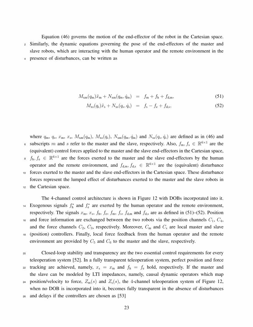
Equation (46) governs the motion of the end-effector of the robot in the Cartesian space.Similarly, the dynamic equations governing the pose of the end-effectors of the master and2

slave robots, which are interacting with the human operator and the remote environment in thepresence of disturbances, can be written as4

Mxm(qm)xm +Nxm(qm, qm) = fm + fh + fd,m, (51)

Mxs(qs)xs +Nxs(qs, qs) = fs − fe + fd,s, (52)

where qm, qs, xm, xs, Mxm(qm), Mxs(qs), Nxm(qm, qm) and Nxs(qs, qs) are defined as in (46) andsubscripts m and s refer to the master and the slave, respectively. Also, fm, fs ∈ R6×1 are the6

(equivalent) control forces applied to the master and the slave end-effectors in the Cartesian space,fh, fe ∈ R6×1 are the forces exerted to the master and the slave end-effectors by the human8

operator and the remote environment, and fd,m, fd,s ∈ R6×1 are the (equivalent) disturbanceforces exerted to the master and the slave end-effectors in the Cartesian space. These disturbance10

forces represent the lumped effect of disturbances exerted to the master and the slave robots inthe Cartesian space.12

The 4-channel control architecture is shown in Figure 12 with DOBs incorporated into it.Exogenous signals f ∗h and f ∗e are exerted by the human operator and the remote environment,14

respectively. The signals xm, xs, fh, fe, fm, fs, fd,m and fd,s are as defined in (51)–(52). Positionand force information are exchanged between the two robots via the position channels C1, C4,16

and the force channels C2, C3, respectively. Moreover, Cm and Cs are local master and slave(position) controllers. Finally, local force feedback from the human operator and the remote18

environment are provided by C5 and C6 to the master and the slave, respectively.

Closed-loop stability and transparency are the two essential control requirements for every20

teleoperation system [52]. In a fully transparent teleoperation system, perfect position and forcetracking are achieved, namely, xs = xm and fh = fe hold, respectively. If the master and22

the slave can be modeled by LTI impedances, namely, causal dynamic operators which mapposition/velocity to force, Zm(s) and Zs(s), the 4-channel teleoperation system of Figure 12,24

when no DOB is incorporated into it, becomes fully transparent in the absence of disturbancesand delays if the controllers are chosen as [53]26

23

C1 = Zs + Cs,

C2 = I + C6,

C3 = I + C5,

C4 = −Zm − Cm. (53)

Extending the idea of DOB-based control of a single robot to a master-slave teleoperationsystem, a DOB for each of the master and slave robots are designed in order to estimate and2

cancel out the disturbances. The 4-channel architecture with NDOBs incorporated into it areshown in Figure 12.4

The vectors fd,m and fd,s denote the master and slave disturbance estimates, respectively.These estimates are employed in a feedforward manner in the following nonlinear control laws6

for the master and slave robots described by (51) and (52), respectively:

fm = Mxm(qm)[−Cmxm − C2fe − C4xs + C6fh + fh]

+Nxm(qm, qm)− fh − fd,m, (54)

fs = Mxs(qs)[−Csxs + C1xm + C3fh − C5fe − fe]

+Nxs(qs, qs) + fe − fd,s, (55)

where Cm, Cs, C1, . . . , and C6 are some LTI controllers satisfying the transparency condition8

in (53).

The DOB-based control laws (54) and (55), when applied to the master and slave described10

by (51)–(52), yield the following closed-loop equations for the master and slave:

xm = −Cmxm − C2fe − C4xs + C6fh

+fh +M−1xm (qm)∆fd,m, (56)

xs = −Csxs + C1xm + C3fh − C5fe

−fe +M−1xs (qs)∆fd,s, (57)

where ∆fd,m = fd,m − fd,m and ∆fd,s = fd,s − fd,s are the master and the slave disturbance12

estimation errors, respectively. Under perfect disturbance tracking, namely, when ∆fd,m = 0

24

and ∆fd,s = 0, (56) and (57) describe an N -DOF conventional disturbance-free 4-channelteleoperation system where the master and slave robots are given by identity inertia matrices,2

namely, Zm(s) = s2I and Zs(s) = s2I .

When the master and slave local position controllers in (54) and (55) are of proportional-4

derivative type, then

Cm = Kmvs+Kmp,

Cs = Ksvs+Ksp, (58)

where Kmv, Kmp, Ksv and Ksp are constant gain matrices. Also, the force reflection gains in (54)6

and (55) are chosen to be

C2 = Cmf,

C3 = Csf, (59)

where Cmf and Csf are constant force reflection gain matrices. The other controllers in (54) and8

(55) are chosen to satisfy the full transparency conditions given by (53). Accordingly,

C1 = s2I +Ksvs+Ksp,

C4 = −(s2I +Kmvs+Kmp),

C5 = Csf − I,

C6 = Cmf − I. (60)

Implementing the controllers C1 and C4 in (60) require measurement or computation of10

acceleration of the master and slave robots. When only good low-frequency transparency isenough for the desired application, the acceleration terms can be omitted. However, requiring12

good transparency over both low and high frequencies justifies using accelerometers [52].Alternatively, precise numerical differentiation techniques may be employed, which are robust14

to measurement errors and input noises, in order to obtain acceleration and velocity signals fromposition measurements [63].16

Using (58), (59), and (60) in (54)–(55) yields the control laws

25

fm = Mxm(qm)[xs −Kmv∆x−Kmp∆x+ Cmf∆f ]

+Nxm(qm, qm)− fh − fd,m, (61)

fs = Mxs(qs)[xm +Ksv∆x+Ksp∆x+ Csf∆f ]

+Nxs(qs, qs) + fe − fd,s, (62)

where ∆x = xm − xs and ∆f = fh − fe are the position and force tracking errors, respectively.Under the control laws (61) and (62), the master and slave closed-loop dynamics (56) and (57)2

are governed by

∆x = −Kmv∆x−Kmp∆x+ Cmf∆f +M−1xm (qm)∆fd,m

(63)

∆x = Ksv∆x+Ksp∆x− Csf∆f −M−1xs (qs)∆fd,s (64)

It is assumed that matrices Cmf, Csf and C−1mf + C−1

sf are invertible. Consequently, multiplying4

(63) and (64) by C−1mf and C−1

sf , respectively and adding them together, the dynamic equationgoverning the position tracking error reads as6

∆x+Kv∆x+Kp∆x = Ψxm(qm)∆fd,m −Ψxs(qs)∆fd,s, (65)

where

Kv = (C−1mf + C−1

sf )−1(C−1sf Ksv − C−1

mf Kmv)

(66)

Kp = (C−1mf + C−1

sf )−1(C−1sf Ksp − C−1

mf Kmp),

Ψxm(qm) = (C−1mf + C−1

sf )−1C−1mf M

−1xm (qm) (67)

Ψxs(qs) = (C−1mf + C−1

sf )−1C−1sf M

−1xs (qs), . (68)

As mentioned before, the need for full transparency in a wide frequency range that8

is required by the transparency conditions in (53) for use in (61) and (62) justifies usingaccelerometers. Consequently, the acceleration measurements, which are used by the conventional10

26

4-channel controllers, are employed in order to simplify NDOB design. Given the master andslave dynamics (51)–(52), the following NDOBs are employed in the 4-channel teleoperation2

architecture

˙fd,m = −Lmfd,m + Lm[Mxm(qm)xm +Nxm(qm, qm)

−fh − fm] + ΨTxm(qm)(∆x+ γ∆x), (69)

˙fd,s = −Lsfd,s + Ls[Mxs(qs)xs +Nxs(qs, qs)

+fe − fs] + ΨTxs(qs)(−∆x− γ∆x), (70)

where γ is an arbitrary positive constant. Also, Lm and Ls are constant gain matrices. As it can4

be seen from (69) and (70), NDOB gains Lm and Ls are constant and there is no need for theauxiliary vector p(.) in the NDOB dynamics. It is remarked that knowing the acceleration signals6

from accelerometers that are employed in the conventional 4-channel teleoperation simplifies thestructure of NDOB gain matrices in comparison with the NDOB structure used in the previous8

sections.

In the conventional 4-channel teleoperation control architecture, human and environmental10

forces, namely, fh and fe, are measured. Equations (51) and (52), along with (69) and (70),result in the following disturbance estimation error dynamics:12

˙fd,m = Lm∆fd,m + ΨT

xm(qm)(∆x+ γ∆x), (71)˙fd,s = Ls∆ds + ΨT

xs(qs)(−∆x− γ∆x). (72)

Therefore, the following disturbance estimation error dynamics result from (71) and (72) for themaster and the slave, respectively:14

∆fd,m = fd,m − Lm∆fd,m −ΨTxm(qm)(∆x+ γ∆x)︸ ︷︷ ︸

ζm

, (73)

∆fd,s = fd,s − Ls∆fd,s −ΨTxs(qs)(−∆x− γ∆x)︸ ︷︷ ︸

ζs

. (74)

It is remarked that the terms ζm = ΨTxm(qm)(∆x + γ∆x) and ζs = ΨT

xs(qs)(−∆x − γ∆x) areemployed in the NDOBs in order to improve the performance of the teleoperation system.16

27

To analyze the performance of this NDOB-based 4-channel architecture, the candidateLyapunov function2

V (∆x,∆x,∆dm,∆ds) =1

2(∆x+ γ∆x)T (∆x+ γ∆x)

+1

2∆xT (Kp + γKv − γ2I)∆x+

1

2∆dTm∆dm +

1

2∆dTs ∆ds,

is considered. Taking its derivative yields

V ≤ −κ0|e|2 + ξ0|e|, (75)

where e = [∆xT ,∆xT ,∆fTd,m,∆fTd,s]

T , κ0 = minλmin(Kv−γI), γλmin(Kp), λmin(Lm), λmin(Ls),4

and ξ0 is some constant that is proportional to the rate of change of the lumped disturbances fd,m

and fd,s (see [49] for further details). It immediately follows that the disturbance and position6

tracking errors of the teleoperation system are globally uniformly ultimately bounded (see “BriefReview of Nonlinear Systems”) and converge with an exponential rate proportional to κ0 to an8

open ball centered at the origin with a radius proportional to 1κ0

. Since κ0 can be made arbitrarilylarge by tuning the design parameters, the 4-channel teleoperation architecture using NDOBs is10

practically stable.

NDOB-based 4-channel teleoperation simulations12

In this section, computer simulations will illustrate effectiveness of the proposed NDOB in4-channel teleoperation subject to disturbances. Both the master and slave robots are considered14

to be planar two-link manipulators with revolute joints. Figure 13 depicts schematic diagram ofthe teleoperation system.16

The Cartesian dynamics of the manipulators are described by [64]

Mx(q) =

[m2 + m1

s220

0 m2

],

Vx(q, q) =

[Vx1(q, q)

Vx2(q, q)

],

28

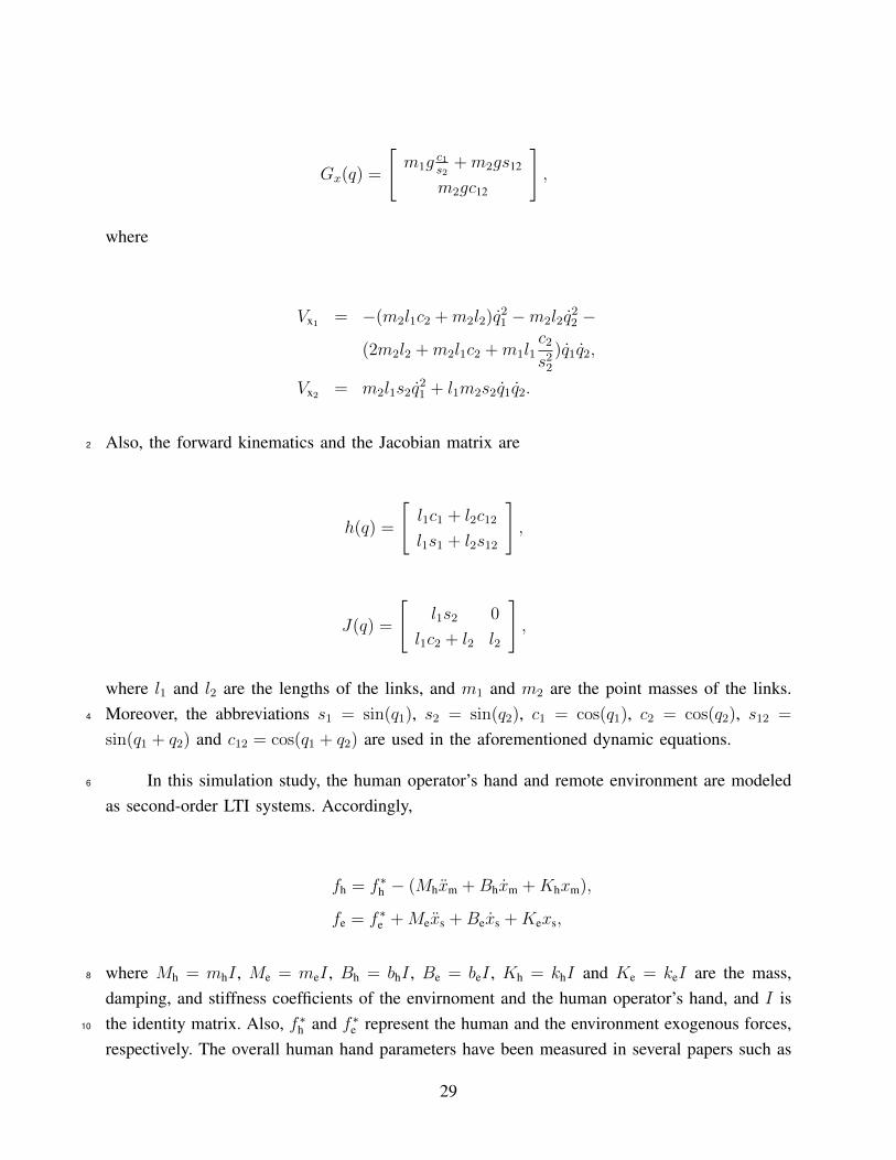
Gx(q) =

[m1g

c1s2

+m2gs12

m2gc12

],

where

Vx1 = −(m2l1c2 +m2l2)q21 −m2l2q

22 −

(2m2l2 +m2l1c2 +m1l1c2

s22

)q1q2,

Vx2 = m2l1s2q21 + l1m2s2q1q2.

Also, the forward kinematics and the Jacobian matrix are2

h(q) =

[l1c1 + l2c12

l1s1 + l2s12

],

J(q) =

[l1s2 0

l1c2 + l2 l2

],

where l1 and l2 are the lengths of the links, and m1 and m2 are the point masses of the links.Moreover, the abbreviations s1 = sin(q1), s2 = sin(q2), c1 = cos(q1), c2 = cos(q2), s12 =4

sin(q1 + q2) and c12 = cos(q1 + q2) are used in the aforementioned dynamic equations.

In this simulation study, the human operator’s hand and remote environment are modeled6

as second-order LTI systems. Accordingly,

fh = f ∗h − (Mhxm +Bhxm +Khxm),

fe = f ∗e +Mexs +Bexs +Kexs,

where Mh = mhI , Me = meI , Bh = bhI , Be = beI , Kh = khI and Ke = keI are the mass,8

damping, and stiffness coefficients of the envirnoment and the human operator’s hand, and I isthe identity matrix. Also, f ∗h and f ∗e represent the human and the environment exogenous forces,10

respectively. The overall human hand parameters have been measured in several papers such as

29

[65], [66] and [67]. In the simulations, the human hand parameters are chosen as in [66]. Theremote environment is modeled by dampers and springs. Accordingly,2

mh = 11.6kg, bh = 17Nsm−1, kh = 243Nm−1,

be = 5Nsm−1, ke = 1Nm−1.

The friction torques acting on the joints of the robots are generated based on the modelin [68]. For the ith joint of the robot, i = 1, 2, the frictions can be modeled as4

τifriction= Fcisgn(qi)[1− exp(

−q2i

v2

si)]

+Fsisgn(qi) exp(−q2

i

v2

si) + Fviqi,

where Fci, Fsi, Fvi are the Coulomb, static, and viscous friction coefficients, respectively. Theparameter vsi is the Stribeck parameter. In the simulations, the friction coefficients and the6

Stribeck parameter for the master and the slave are chosen as follows [69]:

Fci = 0.49, Fsi = 3.5, Fvi = 0.15, vsi = 0.189, i = 1, 2.

The actual parameter values of the master and the slave robots are taken to be8

m1m = 2.3kg, m2m = 2.3kg, l1m = 0.5m, l2m = 0.5m,

m1s = 1.5kg, m2s = 1.5kg, l1s = 0.5m, l2s = 0.5m.

Assuming a maximum of ±25% uncertainty in these parameters, the approximate values of thesemaster and the slave parameters are taken to be10

m1m = 2.82kg, m2m = 2.36kg, l1m = 0.62m, l2m = 0.56m,

m1s = 1.16kg, m2s = 1.29kg, l1s = 0.38m, l2s = 0.52m.

30

The controllers Cm, Cs, C1, . . . , and C6 are chosen as in (58), (59) and (60). The controllersand DOB gains and initial conditions are chosen as2

γ = 1,

Kmv = 50I , Ksv = 50I,

Kmp = 50I , Ksp = 50I,

Cmf = I , Csf = I,

Lm = 50I , Ls = 50I,

fd,m(0) = 0 , fd,s(0) = 0,

Kv = 25I , Kp = 25I.

It is to be noted that the master and slave controller and observer gains have been chosen tobe equal– this choice is not necessary but is one that results in identical closed-loop master and4

slave dynamics (63) and (64) when ∆dm = 0 and ∆ds = 0.

Different values for initial joint positions of the master and the slave are chosen while6

assuming that both robots are initially at rest. The initial joint position vectors are taken to be

q0m = [30, 45]T ,

q0s = [0, 22.5]T .

In the simulations, f ∗e = [0, 0]T and it is assumed that the human operator moves the master8

end-effector such that the second joint of the master robot moves from 45 to 81.5 while theposition of the first joint of the master robot is fixed. The slave end-effector should follow the10

position of the master end-effector. It is assumed that an external payload, with a mass equalto 0.5kg, is connected to the end-effector of the slave. Also, it is assumed that a sinusoidal12

disturbance torque equal to τd = sin(4πt) is exerted to the second joint of the slave robot.Sinusoidal disturbances are exerted to the joints of a robot in order to examine the efficiency of14

fault tolerant control schemes.

Figures 14 and 15 show the position tracking responses of the teleoperation system in16

presence and absence of the NDOBs. Because of the sinusoidal disturbance acting on the secondjoint of the slave robot, the slave robot end-effector payload, the friction forces and the dynamic18

uncertainties present in the master and the slave model, the control law without using DOBsfails to achieve good position tracking. As it can be observed from Figures 14 and 15, perfect20

position tracking has been achieved under the DOB-based control scheme while there are offsets

31

in the position tracking error under the conventional control scheme. Figure 16 shows the forcetracking responses of the teleoperation system in presence and absence of the NDOBs. Figures2

17 and 18 show the disturbance tracking of the DOB at the master and the slave sides. As it canbe observed from these figures, the disturbances are not constant at the slave side. However, the4

estimated disturbances tend to follow the actual disturbances with a bounded tracking error.

Future Research Directions6

Despite the success of NDOBs in numerous applications, there is a need to expandtheoretical studies in this field. There are numerous future research directions that have been8

highlighted in [11]. The following directions may also be considered in expanding the DOBframework.10

• Extending the NDOB framework to hybrid dynamical control systems: Hybrid dynamicalcontrol systems are a class of control systems that possess both continuous and discrete12

dynamics [70], [71]. Power systems and mechanical systems subject to impulsive contactsare a few examples that can be modeled as hybrid dynamical systems that are subject to14

numerous disturbances. The disturbance observer literature is also rich in the context ofdiscrete-time dynamical systems (see [72] and the references therein). However, to the best16

knowledge of the authors, there has not been any studies regarding the applicability ofDOBs to the hybrid settings.18

• Generalizing the NDOB framework from dynamical systems with Euclidean state-spaces tosystems with curved state-spaces: The NDOB framework has thus far been studied in the20

context of dynamical control systems with Euclidean state-spaces. However, there are manydynamical control systems such as underwater and ground vehicles subject to disturbances22

whose state-space are not Euclidean [73]. The NDOB framework can be extended toaccompany global controllers that are designed for this class of systems.24

• Using NDOBs in underactuated mechanical systems: Underactuation is a pervasive phe-nomenon in robotic locomotory systems such as legged robots. Theses systems are subject26

to various disturbances as they locomote in their ambient environment. Therefore, NDOBsseem to be suitable candidates for disturbance attenuation in these applications. Relaxing28

the matching condition is an important challenge that arises in the context of underactuatedrobotics. Early progress has been made to address this challenge in [24].30

• Input observability analysis for NDOBs: the important analysis of input observability and itsgeometric interpretation has been largely ignored by the NDOB community. One important32

reason might be that developing a nonlinear counterpart of matrix pencil decompositionsthat are used for input observability analysis in LTI systems in [74], is a difficult task.34

32

The input observability analysis is a research direction that NDOB community needs toinvestigate further.2

Concluding Remarks

This article discussed a class of unknown input observers called the nonlinear disturbance4

observers than can be effectively used in control of robotic and teleoperation systems. Numerouscommercial applications of DOBs motivate further theoretical investigation of this class of6

observers. In this article, several inherent properties of the NDOB proposed in [21] that were notdiscussed in the previous NDOB literature such as semi/quasi-passivity were shown. Exploiting8

the inherent properties of EL systems, it was shown that NDOBs can be employed along withpassivity-based and computed-torque control schemes without the need to modify these well-10

established controllers. Applications of NDOBs in the 4-channel teleoperation architecture, whichguarantees transparency in the absence of disturbances, were investigated in this article.12

References

[1] A. Radke and Z. Gao, “A survey of state and disturbance observers for practitioners,” in14

Proc. American Control Conference, 2006, pp. 5183–5188.

[2] K. Ohishi, K. Ohnishi, and K. Miyachi, “Torque-speed regulation of dc motor based on16

load torque estimation,” in Proc. Int. Conf. IEEJ IPEC, 1983, pp. 1209–1216.

[3] X. Chen, J. Yang, S. Li, and Q. Li, “Disturbance observer based multi-variable control of18

ball mill grinding circuits,” J. Process Contr., vol. 19, no. 7, pp. 1205–1213, 2009.

[4] J. Yang, S. Li, X. Chen, and Q. Li, “Disturbance rejection of dead-time processes using20

disturbance observer and model predictive control,” Chem. Eng. Res. Des., vol. 89, no. 2,pp. 125–135, 2011.22

[5] K. Ohnishi, M. Shibata, and T. Murakami, “Motion control for advanced mechatronics,”IEEE/ASME Trans. Mechatron., vol. 1, no. 1, pp. 56–67, Mar. 1996.24

[6] Y. Oh and W. K. Chung, “Disturbance-observer-based motion control of redundantmanipulators using inertially decoupled dynamics,” IEEE/ASME Trans. Mechatron., vol. 4,26

no. 2, pp. 133–146, 1999.

[7] P. K. Sinha and A. N. Pechev, “Model reference adaptive control of a maglev system with28

stable maximum descent criterion,” Automatica, vol. 35, no. 8, pp. 1457–1465, 1999.

[8] P. Zhang and S. X. Ding, “Disturbance decoupling in fault detection of linear periodic30

systems,” Automatica, vol. 43, no. 8, pp. 1410–1417, 2007.

[9] B. A. Guvenc, L. Guvenc, and S. Karaman, “Robust mimo disturbance observer analysis32

and design with application to active car steering,” Int. J. Robust Nonlinear Control, vol. 20,

33

pp. 873–891, 2010.

[10] S. Li, J. Yang, W.-h. Chen, and X. Chen, Disturbance observer-based control: methods2

and applications. CRC press, 2014.

[11] W.-H. Chen, J. Yang, L. Guo, and S. Li, “Disturbance observer-based control and4

related methods: An overview,” IEEE Trans. Ind. Electron., 2015, to appear, DOI:10.1109/TIE.2015.2478397.6

[12] K. Ohnishi, “A new servo method in mechatronics,” Trans. Japan Society of ElectricalEngineering, vol. 107-D, pp. 83–86, 1987.8

[13] T. Murakami, F. M. Yu, and K. Ohnishi, “Torque sensorless control in multidegree-of-freedom manipulator,” IEEE Trans. Ind. Electron., vol. 40, no. 2, pp. 259–265, Apr. 1993.10

[14] C. S. Liu and H. Peng, “Disturbance observer based tracking control,” ASME Trans. Dyn.Syst. Meas. Control, vol. 122, no. 2, pp. 332–335, Jun. 2000.12

[15] Q.-C. Zhong and J. E. Normey-Rico, “Control of integral processes with dead-time. part1: Disturbance observer-based 2dof control scheme,” IEE Proceedings-Control Theory and14

Applications, vol. 149, no. 4, pp. 285–290, 2002.

[16] K. Natori, T. Tsuji, K. Ohnishi, A. Hace, and K. Jezernik, “Time-delay compensation by16

communication disturbance observer for bilateral teleoperation under time-varying delay,”IEEE Trans. Ind. Electron., vol. 57, no. 3, pp. 1050–1062, Mar. 2010.18

[17] E. Sariyildiz and K. Ohnishi, “Stability and robustness of disturbance-observer-basedmotion control systems,” IEEE Trans. Ind. Electron., vol. 62, no. 1, pp. 414–422, 2015.20

[18] ——, “A guide to design disturbance observer,” J. Dyn. Syst. Meas. Control, vol. 136, no. 2,2014.22

[19] K.-S. Kim, K.-H. Rew, and S. Kim, “Disturbance observer for estimating higher orderdisturbances in time series expansion,” IEEE Trans. Automat. Contr., vol. 55, no. 8, pp.24

1905–1911, 2010.

[20] X. Chen, S. Komada, and T. Fukuda, “Design of a nonlinear disturbance observer,” IEEE26

Trans. Ind. Electron., vol. 47, no. 2, pp. 429–437, 2000.

[21] W.-H. Chen, “Disturbance observer based control for nonlinear systems,” IEEE/ASME28

Trans. Mechatron., vol. 9, no. 4, pp. 706–710, 2004.

[22] X. Chen, C.-Y. Su, and T. Fukuda, “A nonlinear disturbance observer for multivariable30

systems and its application to magnetic bearing systems,” IEEE Trans. Contr. Syst. Technol.,vol. 12, no. 4, pp. 569–577, 2004.32

[23] J. Back and H. Shim, “Adding robustness to nominal output-feedback controllers foruncertain nonlinear systems: A nonlinear version of disturbance observer,” Automatica,34

vol. 44, no. 10, pp. 2528–2537, 2008.

[24] J. Yang, S. Li, and W.-H. Chen, “Nonlinear disturbance observer-based control for multi-36

34

input multi-output nonlinear systems subject to mismatching condition,” Int. J. Contr.,vol. 85, no. 8, pp. 1071–1082, 2012.2

[25] H. Shim and N. H. Jo, “An almost necessary and sufficient condition for robust stability ofclosed-loop systems with disturbance observer,” Automatica, vol. 45, no. 1, pp. 296–299,4

2009.[26] J. Back and H. Shim, “An inner-loop controller guaranteeing robust transient performance6

for uncertain mimo nonlinear systems,” IEEE Trans. Automat. Contr., vol. 54, no. 7, pp.1601–1607, 2009.8

[27] S. Lichiardopol, N. van de Wouw, D. Kostic, and H. Nijmeijer, “Trajectory tracking controlfor a tele-operation system setup with disturbance estimation and compensation,” in Proc.10

IEEE Conf. Decision and Control, 2010, pp. 1142–1147.[28] A. Nikoobin and R. Haghighi, “Lyapunov-based nonlinear disturbance observer for serial12

n-link robot manipulators,” J. Intell. Robot. Syst., vol. 55, no. 2-3, pp. 135–153, Jul. 2009.[29] A. Mohammadi, M. Tavakoli, H. J. Marquez, and F. Hashemzadeh, “Nonlinear disturbance14

observer design for robotic manipulators,” Control Eng. Pract., vol. 21, no. 3, pp. 253–267,2013.16

[30] R. Hao, J. Wang, J. Zhao, and S. Wang, “Observer-based robust control of 6-dof parallelelectrical manipulator with fast friction estimation,” IEEE Trans. Autom. Sci. Eng., 2015,18

to appear. DOI: 10.1109/TASE.2015.2427743.[31] M. Kim and D. Lee, “Toward transparent virtual coupling for haptic interaction during20

contact tasks,” in Proc. World Haptics Conference, 2013, pp. 163–168.[32] T. Floquet, J.-P. Barbot, W. Perruquetti, and M. Djemai, “On the robust fault detection via22

a sliding mode disturbance observer,” Int. J. Contr., vol. 77, no. 7, pp. 622–629, 2004.[33] X.-G. Yan and C. Edwards, “Nonlinear robust fault reconstruction and estimation using a24

sliding mode observer,” Automatica, vol. 43, no. 9, pp. 1605–1614, 2007.[34] C. E. Hall and Y. B. Shtessel, “Sliding mode disturbance observer-based control for a26

reusable launch vehicle,” Journal of guidance, control, and dynamics, vol. 29, no. 6, pp.1315–1328, 2006.28

[35] L. Besnard, Y. B. Shtessel, and B. Landrum, “Quadrotor vehicle control via sliding modecontroller driven by sliding mode disturbance observer,” Journal of the Franklin Institute,30

vol. 349, no. 2, pp. 658–684, 2012.[36] T. E. Massey and Y. B. Shtessel, “Continuous traditional and high-order sliding modes for32

satellite formation control,” Journal of Guidance, Control, and Dynamics, vol. 28, no. 4,pp. 826–831, 2005.34

[37] A. A. Godbole, J. P. Kolhe, and S. E. Talole, “Performance analysis of generalized extendedstate observer in tackling sinusoidal disturbances,” Control Systems Technology, IEEE36

Transactions on, vol. 21, no. 6, pp. 2212–2223, 2013.

35

[38] S. Li, J. Yang, W.-H. Chen, and X. Chen, “Generalized extended state observer based controlfor systems with mismatched uncertainties,” Industrial Electronics, IEEE Transactions on,2

vol. 59, no. 12, pp. 4792–4802, 2012.[39] W. H. Chen, D. J. Ballance, P. J. Gawthrop, and J. O’Reilly, “A nonlinear disturbance4

observer for robotic manipulators,” IEEE Trans. Ind. Electron., vol. 47, no. 4, pp. 932–938,Aug. 2000.6

[40] A. Mohammadi, H. J. Marquez, and M. Tavakoli, “Disturbance observer based trajectoryfollowing control of nonlinear robotic manipulators,” in Proc. Canadian Congress of8

Applied Mechanics, Vancouver, BC, Jun. 2011.[41] J. Huang, S. Ri, L. Liu, Y. Wang, J. Kim, and G. Pak, “Nonlinear disturbance observer-10

based dynamic surface control of mobile wheeled inverted pendulum,” IEEE Trans. Cont.Syst. Technol., 2015, to appear. DOI: 10.1109/TCST.2015.2404897.12

[42] T.-S. Lee, “Lagrangian modeling and passivity-based control of three-phase ac/dc voltage-source converters,” IEEE Trans. Ind. Electron., vol. 51, no. 4, pp. 892–902, 2004.14

[43] A. Tofighi and M. Kalantar, “Power management of pv/battery hybrid power source viapassivity-based control,” Renewable Energy, vol. 36, no. 9, pp. 2440–2450, 2011.16

[44] J. M. Scherpen, D. Jeltsema, and J. B. Klaassens, “Lagrangian modeling of switchingelectrical networks,” Systems & Control Letters, vol. 48, no. 5, pp. 365–374, 2003.18

[45] M. W. Spong, S. Hutchinson, and M. Vidyasagar, Robot Modeling and Control. NewYork: Wiley, 2005.20

[46] H. Amini, S. Rezaei, A. A. Sarhan, J. Akbari, and N. Mardi, “Transparency improvementby external force estimation in a time-delayed nonlinear bilateral teleoperation system,” J.22

Dyn. Syst. Meas. Control, vol. 137, no. 5, p. 051013, 2015.[47] A. Mohammadi, M. Tavakoli, and H. J. Marquez, “Control of nonlinear bilateral teleoper-24

ation systems subject to disturbances,” in IEEE 50th Conference on Decision and Control,2011, pp. 1765–1770.26

[48] N. Iiyama, K. Natori, and K. Ohnishi, “Bilateral teleoperation under time-varying communi-cation time delay considering contact with environment,” Electronics and Communications28

in Japan, vol. 92, no. 7, pp. 38–46, 2009.[49] A. Mohammadi, M. Tavakoli, and H. J. Marquez, “Disturbance observer based control30

of nonlinear haptic teleoperation systems,” IET Control Theory Appl., vol. 5, no. 17, pp.2063–2074, 2011.32

[50] ——, “Control of nonlinear teleoperation systems subject to disturbances and variable timedelays,” in Proc. IEEE/RSJ Int. Conf. Intell. Robot. Syst., 2012, pp. 3017–3022.34

[51] T. B. Sheridan, “Telerobotics,” Automatica, vol. 25, no. 4, pp. 487–507, Jul. 1989.[52] D. A. Lawrence, “Stability and transparency in bilateral teleoperation,” IEEE Trans. Robot.36

Autom., vol. 9, pp. 624–637, Oct. 1993.

36

[53] M. Tavakoli, A. Aziminejad, R. Patel, and M. Moallem, “High-fidelity bilateral teleoperationsystems and the effect of multimodal haptics,” IEEE Trans. Syst., Man Cybern. B, bern.,2

vol. 37, no. 6, pp. 1512–1528, Dec. 2007.

[54] P. Hokayem and M. W. Spong, “Bilateral teleoperation: An historical survey,” Automatica,4

vol. 42, pp. 2035–2057, 2006.

[55] E. Sariyildiz, “Advanced robust control via disturbance observer: Implementations in the6

motion control framework,” Ph.D. dissertation, Keio University, 2014.

[56] W.-H. Chen and L. Guo, “Analysis of disturbance observer based control for nonlinear8

systems under disturbances with bounded variation,” in Proc. Int. Conf. Contr., 2004.

[57] H. K. Khalil, Nonlinear Systems. Upper Saddle River, NJ: Prentice Hall, 3rd edn, 2002.10

[58] A. Abdessameud, I. G. Polushin, and A. Tayebi, “Synchronization of Lagrangian systemswith irregular communication delays,” IEEE Trans. Automat. Contr., vol. 59, no. 1, pp.12

187–193, 2014.

[59] A. Mohammadi, M. Tavakoli, and A. Jazayeri, “PHANSIM: A Simulink toolkit for the14

SensAble haptic devices,” in Proc. Canadian Congress of Applied Mechanics, Vancouver,BC, Jun. 2011, pp. 787–790.16

[60] S. Katsura, Y. Matsumoto, and K. Ohnishi, “Modeling of force sensing and validation ofdisturbance observer for force control,” in Proc. IEEE Conf. Ind. Electron. Society, 2003,18

pp. 291–296.

[61] K. Natori, T. Tsuji, and K. Ohnishi, “Time delay compensation by communication20

disturbance observer in bilateral teleoperation systems,” in Proc. IEEE Int. Workshop Adv.Motion Control, 2006, pp. 218–223.22

[62] S. Katsura, Y. Matsumoto, and K. Ohnishi, “Shadow robot for teaching motion,” Robot.Auton. Syst., vol. 58, no. 7, pp. 840–846, Jul. 2010.24

[63] A. Levant, “Robust exact differentiation via sliding mode technique,” Automatica, vol. 34,no. 3, pp. 379–384, Mar. 1998.26

[64] J. J. Craig, Introduction to Robotics: Mechanics and Control. Upper Saddle River, NJ:Pearson Prentice Hall, 2005.28

[65] W. H. Zhu and S. E. Salcudean, “Stability guaranteed teleoperation: An adaptive mo-tion/force control approach,” IEEE Trans. Autom. Control, vol. 45, no. 11, pp. 1951–1969,30

Nov. 2000.

[66] K. Kosuge, Y. Fujisawa, and T. Fukuda, “Control of mechanical system with man-machine32

interaction,” in Proc. IEEE/RSJ Int. Conf. Intell. Robots Syst., 1992, pp. 87–92.

[67] J. E. Speich, L. Shao, and M. Goldfarb, “Modeling the human hand as it interacts with a34

telemanipulation system,” Mechatronics, vol. 15, no. 9, pp. 1127–1142, 2005.

[68] B. Armstrong-Helouvry, P. Dupont, and C. Canudas-de Wit, “A survey of models, analysis36

37

tools and compensation methods for the control of machines with friction,” Automatica,vol. 30, no. 7, pp. 1083–1138, 1994.2

[69] N. Hung, H. Tuan, T. Narikiyo, and P. Apkarian, “Adaptive control for nonlinearlyparameterized uncertainties in robot manipulators,” IEEE Trans. Cont. Syst. Technol.,4

vol. 16, no. 3, pp. 458–468, 2008.[70] A. J. Van Der Schaft and J. M. Schumacher, An introduction to hybrid dynamical systems.6

Springer London, 2000, vol. 251.[71] R. Goebel, R. G. Sanfelice, and A. Teel, “Hybrid dynamical systems,” IEEE Control8

Systems, vol. 29, no. 2, pp. 28–93, 2009.[72] K.-S. Kim and K.-H. Rew, “Reduced order disturbance observer for discrete-time linear10

systems,” Automatica, vol. 49, no. 4, pp. 968–975, 2013.[73] N. A. Chaturvedi, A. K. Sanyal, and N. H. McClamroch, “Rigid-body attitude control,”12

IEEE Control Systems, vol. 31, no. 3, pp. 30–51, 2011.[74] M. Hou and R. J. Patton, “Input observability and input reconstruction,” Automatica, vol. 34,14

no. 6, pp. 789–794, 1998.[75] E. Naerum, J. Cornella, and O. J. Elle, “Contact force estimation for backdrivable robotic16

manipulators with coupled friction,” in Proc. IEEE Int. Conf. Intell. Robots Syst., 2008, pp.3021–3027.18

[76] B. Taati, A. M. Tahmasebi, and K. Hashtrudi-Zaad, “Experimental identification andanalysis of the dynamics of a phantom premium 1.5a hatpic device,” Presence, vol. 17,20

no. 4, pp. 327–342, Aug. 2008.[77] T. Soderstrom and P. Stoica, System Identification. Prentice Hall International Ltd, 1989.22

[78] K. J. Astrom and B. Wittenmark, Adatpive Control. Addison Wesley, 1995.

38

List of Figures

1 Block diagram of a typical disturbance observer in a control system. The unknown2

disturbances that are acting on the plant are reconstructed from the measured outputvariables and the known control inputs applied to the system by the disturbance4

observer. The output of the disturbance observer, namely, the estimated disturbance,can then be used in feedforward compensation of disturbances or fault detection. . 436

2 A typical teleoperation system. Teleoperation involves indirect performance of a taskin a remote environment and is used to extend a person’s sensing and manipulation8

capability to a remote location. Every teleoperation system consists of a master robot(user interface) and a slave robot, which exchange different types of information10

such as force, position, and visual and auditory data via a communication channel. 44

3 Block diagram of a disturbance observer-based robust motion control system12

proposed in [2], [12]. The unknown disturbance τd lumps the effect of externaldisturbances and plant uncertainties, such as inertia variation and friction. The14

control input is represented by the torque τ . The parameters J and Ld representmass/inertia and gain of the disturbance observer (DOB), which is a design16

parameter, respectively. . . . . . . . . . . . . . . . . . . . . . . . . . . . . . . . . . 45

4 Block diagram of the nonlinear disturbance observer-based robust control system18

proposed in [21]. The disturbance observer estimates the lumped disturbance vectord from the state and input vectors. The vector z ∈ Rl is the internal state vector20

of the disturbance observer. The matrix Ld(x) is called the DOB gain and satisfiesLd(x) = ∂p(x)

∂x. . . . . . . . . . . . . . . . . . . . . . . . . . . . . . . . . . . . . . . 4622

5 The PHANToM Omni hatpic device and the payload attached to its gimbal. ThePHANToM Omni has three actuated revolute joints which provide the user with24

force feedback information. In addition to the actuated joints, the PHANToM robothas three wrist joints that are passive. The first and the third actuated joints of26

the PHANToM robot in experiments will be used while the second actuated jointis locked at 0deg. The PHANToM Omni is connected to the computer through an28

IEEE 1394 port. The PHANToM Omni end-effector position and orientation dataare collected at a frequency of 1 kHz. The payload is a metal cube which is attached30

to the gimbal of the robot. . . . . . . . . . . . . . . . . . . . . . . . . . . . . . . . 47

6 Time profile of position of the first joint of the PHANToM robot. The nonlinear32

disturbance observer (NDOB), accompanying the computed-torque controller in thisexperiment, is used to estimate and compensate for the joint frictions and external34

payload. The payload is a metal cube which is attached to the gimbal of the robot.According to Table 2, the root mean square (RMS) position tracking error of the36

third joint has been significantly improved using the NDOB structure of [21], [39]with NDOB gain given in [29]. . . . . . . . . . . . . . . . . . . . . . . . . . . . . . 4838

39

7 Time profile of position tracking error of the first joint of the PHANToM robot.The nonlinear disturbance observer (NDOB), accompanying the computed-torque2

controller in this experiment, is used to estimate and compensate for the jointfrictions and external payload. The payload is a metal cube which is attached to the4

gimbal of the robot. According to Table 2, the root mean square (RMS) positiontracking error of the third joint has been significantly improved using the NDOB6

structure of [21], [39] with NDOB gain given in [29]. . . . . . . . . . . . . . . . . 49

8 Time profile of position of the third joint of the PHANToM robot. The nonlinear8

disturbance observer (NDOB), accompanying the computed-torque controller in thisexperiment, is used to estimate and compensate for the joint frictions and external10

payload. The payload is a metal cube which is attached to the gimbal of the robot.According to Table 2, the root mean square (RMS) position tracking error of the12

third joint has been significantly improved using the NDOB structure of [21], [39]with NDOB gain given in [29]. . . . . . . . . . . . . . . . . . . . . . . . . . . . . . 5014

9 Time profile of position tracking error of the third joint of the PHANToM robot.The nonlinear disturbance observer (NDOB), accompanying the computed-torque16

controller in this experiment, is used to estimate and compensate for the jointfrictions and external payload. The payload is a metal cube which is attached to the18

gimbal of the robot. According to Table 2, the root mean square (RMS) positiontracking error of the third joint has been significantly improved using the NDOB20

structure of [21], [39] with NDOB gain given in [29]. . . . . . . . . . . . . . . . . 51

10 Time profiles of disturbance tracking for the first joint of the PHANToM robot: (a)22

PHANToM disturbance torque estimation, and (b) PHANToM disturbance torqueestimation errors. The nonlinear disturbance observer (NDOB), accompanying the24

computed-torque controller in this experiment, is used to estimate and compensatefor the joint frictions and external payload. The payload is a metal cube which is26

attached to the gimbal of the robot. According to Table 3, the root mean square(RMS) disturbance tracking error of the third joint has been significantly improved28

using the NDOB structure of [21], [39] with NDOB gain given in [29]. . . . . . . 52

11 Time profiles of disturbance tracking for the third joint of the PHANToM robot: (a)30

PHANToM disturbance torque estimation, and (b) PHANToM disturbance torqueestimation errors. The nonlinear disturbance observer (NDOB), accompanying the32

computed-torque controller in this experiment, is used to estimate and compensatefor the joint frictions and external payload. The payload is a metal cube which is34

attached to the gimbal of the robot. According to Table 3, the root mean square(RMS) disturbance tracking error of the third joint has been significantly improved36

using the NDOB structure of [21], [39] with NDOB gain given in [29]. . . . . . . 53

40

12 Disturbance observer-based (DOB-based) 4-channel teleoperation control system.Exogenous signals f ∗h and f ∗e are exerted by the human operator and the remote2

environment, respectively. The signals xm, xs, fh, fe, fm, fs, fd,m and fd,s are asdefined in (51)–(52). Position information is exchanged between the master and the4

slave via the position channels C1 and C4. Force information is exchanged throughthe force channels C2 and C3. In addition, Cm and Cs are local master and slave6

(position) controllers. Lastly, C5 and C6 provide the master and the slave with localforce feedback from the human operator and the remote environment, respectively. 548

13 Schematic diagram of the teleoperation system used in simulation. Both the masterand the slave robots are considered to be planar two-link manipulators with revolute10

joints. It is assumed that an external payload, with a mass equal to 0.5kg, is connectedto the end-effector of the slave. Also, it is assumed that a sinusoidal disturbance12

torque equal to τd = sin(4πt) is exerted to the second joint of the slave robot. Theseexternal disturbances are exerted to the slave robot in addition to the disturbances14

due to joint frictions and dynamic uncertainties. . . . . . . . . . . . . . . . . . . . . 55

14 Position tracking of the teleoperation system in the Cartesian space in (a) x1 coordi-16

nate, and (b) x2 coordinate, with and without disturbance observer (DOB). Both themaster and the slave robots are considered to be planar two-link manipulators with18

revolute joints. It is assumed that an external payload, with a mass equal to 0.5kg,is connected to the end-effector of the slave. Also, it is assumed that a sinusoidal20

disturbance torque equal to τd = sin(4πt) is exerted to the second joint of the slaverobot. Position tracking errors are smaller when nonlinear disturbance observers22

(NDOBs) are incorporated in the 4-channel teleoperation architecture. . . . . . . . . 56

15 Position tracking error of the teleoperation system in the Cartesian space in24

(a) x1 coordinate, and (b) x2 coordinate, with and without disturbance observer(DOB). Both the master and the slave robots are considered to be planar two-link26

manipulators with revolute joints. It is assumed that an external payload, with a massequal to 0.5kg, is connected to the end-effector of the slave. Also, it is assumed that28

a sinusoidal disturbance torque equal to τd = sin(4πt) is exerted to the second jointof the slave robot. Position tracking errors are smaller when nonlinear disturbance30

observers (NDOBs) are incorporated in the 4-channel teleoperation architecture. . . 57

16 Force tracking of the teleoperation system with and without disturbance observer32

(DOB). One of the features of the 4-channel architecture is its capability ofachieving transparency in the absence of disturbances. As it can be seen from the34

figure, the force tracking is degraded severely in the presence of disturbances thatare not compensated. Force tracking errors are smaller when nonlinear disturbance36

observers (NDOBs) are incorporated in the 4-channel teleoperation architecture. . . 58

17 Disturbance tracking at the slave side in (a) x1 coordinate, and (b) x2 coordinate.38

It is assumed that an external payload, with a mass equal to 0.5kg, is connectedto the end-effector of the slave. Also, it is assumed that a sinusoidal disturbance40

torque equal to τd = sin(4πt) is exerted to the second joint of the slave robot. Thedisturbance tracking errors at the slave side are uniformly ultimately bounded. . . . 5942

41

18 Disturbance tracking at the master side in (a) x1 coordinate, and (b) x2 coordinate.It is assumed that an external payload, with a mass equal to 0.5kg, is connected2

to the end-effector of the slave. Also, it is assumed that a sinusoidal disturbancetorque equal to τd = sin(4πt) is exerted to the second joint of the slave robot. The4

disturbance tracking errors at the master side are uniformly ultimately bounded. . . 60

42

Figure 1: Block diagram of a typical disturbance observer in a control system. The unknown disturbances that areacting on the plant are reconstructed from the measured output variables and the known control inputs applied tothe system by the disturbance observer. The output of the disturbance observer, namely, the estimated disturbance,can then be used in feedforward compensation of disturbances or fault detection.

43

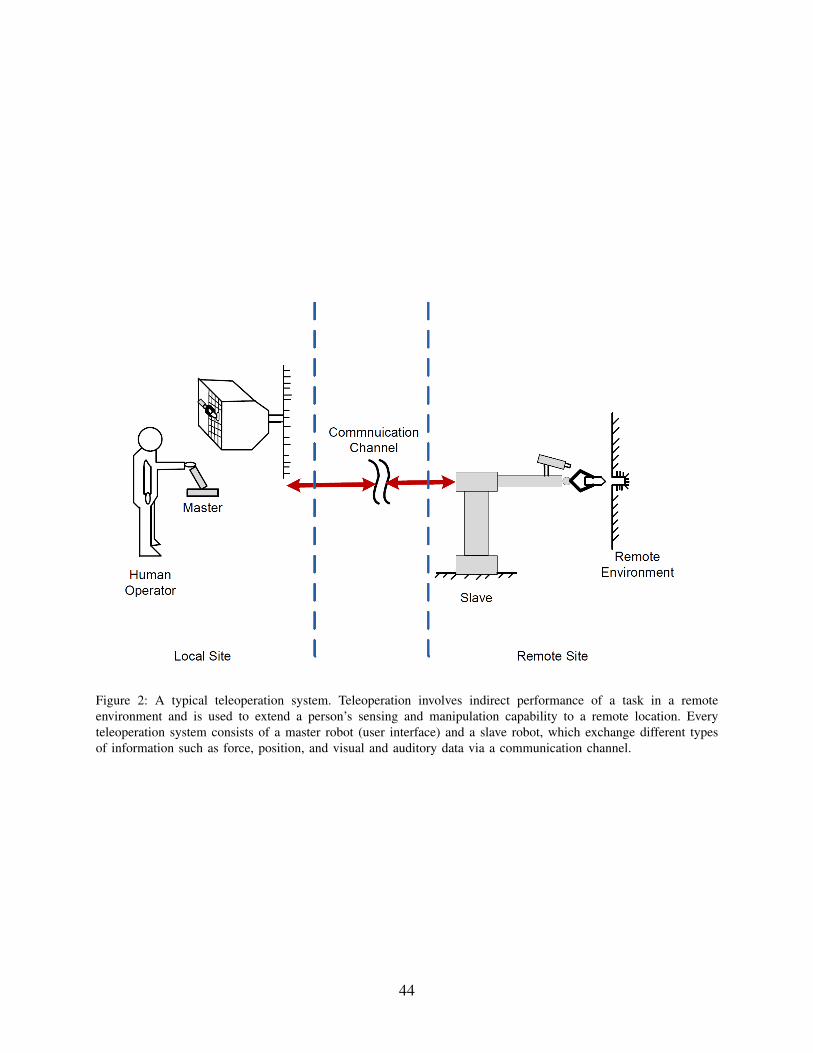
Figure 2: A typical teleoperation system. Teleoperation involves indirect performance of a task in a remoteenvironment and is used to extend a person’s sensing and manipulation capability to a remote location. Everyteleoperation system consists of a master robot (user interface) and a slave robot, which exchange different typesof information such as force, position, and visual and auditory data via a communication channel.

44

Figure 3: Block diagram of a disturbance observer-based robust motion control system proposed in [2], [12]. Theunknown disturbance τd lumps the effect of external disturbances and plant uncertainties, such as inertia variationand friction. The control input is represented by the torque τ . The parameters J and Ld represent mass/inertia andgain of the disturbance observer (DOB), which is a design parameter, respectively.

45

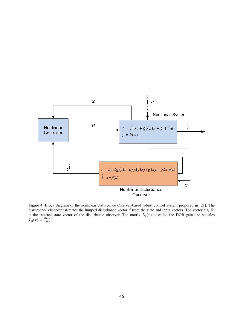
Figure 4: Block diagram of the nonlinear disturbance observer-based robust control system proposed in [21]. Thedisturbance observer estimates the lumped disturbance vector d from the state and input vectors. The vector z ∈ Rl

is the internal state vector of the disturbance observer. The matrix Ld(x) is called the DOB gain and satisfiesLd(x) =

∂p(x)∂x .

46

Figure 5: The PHANToM Omni hatpic device and the payload attached to its gimbal. The PHANToM Omni hasthree actuated revolute joints which provide the user with force feedback information. In addition to the actuatedjoints, the PHANToM robot has three wrist joints that are passive. The first and the third actuated joints of thePHANToM robot in experiments will be used while the second actuated joint is locked at 0deg. The PHANToMOmni is connected to the computer through an IEEE 1394 port. The PHANToM Omni end-effector position andorientation data are collected at a frequency of 1 kHz. The payload is a metal cube which is attached to the gimbalof the robot.

47

Figure 6: Time profile of position of the first joint of the PHANToM robot. The nonlinear disturbance observer(NDOB), accompanying the computed-torque controller in this experiment, is used to estimate and compensate forthe joint frictions and external payload. The payload is a metal cube which is attached to the gimbal of the robot.According to Table 2, the root mean square (RMS) position tracking error of the third joint has been significantlyimproved using the NDOB structure of [21], [39] with NDOB gain given in [29].

48

Figure 7: Time profile of position tracking error of the first joint of the PHANToM robot. The nonlinear disturbanceobserver (NDOB), accompanying the computed-torque controller in this experiment, is used to estimate andcompensate for the joint frictions and external payload. The payload is a metal cube which is attached to thegimbal of the robot. According to Table 2, the root mean square (RMS) position tracking error of the third jointhas been significantly improved using the NDOB structure of [21], [39] with NDOB gain given in [29].

49

Figure 8: Time profile of position of the third joint of the PHANToM robot. The nonlinear disturbance observer(NDOB), accompanying the computed-torque controller in this experiment, is used to estimate and compensate forthe joint frictions and external payload. The payload is a metal cube which is attached to the gimbal of the robot.According to Table 2, the root mean square (RMS) position tracking error of the third joint has been significantlyimproved using the NDOB structure of [21], [39] with NDOB gain given in [29].

50

Figure 9: Time profile of position tracking error of the third joint of the PHANToM robot. The nonlinear disturbanceobserver (NDOB), accompanying the computed-torque controller in this experiment, is used to estimate andcompensate for the joint frictions and external payload. The payload is a metal cube which is attached to thegimbal of the robot. According to Table 2, the root mean square (RMS) position tracking error of the third jointhas been significantly improved using the NDOB structure of [21], [39] with NDOB gain given in [29].

51

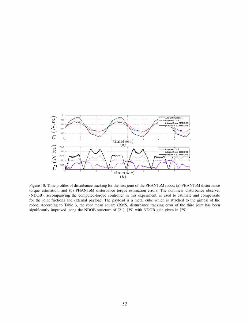
Figure 10: Time profiles of disturbance tracking for the first joint of the PHANToM robot: (a) PHANToM disturbancetorque estimation, and (b) PHANToM disturbance torque estimation errors. The nonlinear disturbance observer(NDOB), accompanying the computed-torque controller in this experiment, is used to estimate and compensatefor the joint frictions and external payload. The payload is a metal cube which is attached to the gimbal of therobot. According to Table 3, the root mean square (RMS) disturbance tracking error of the third joint has beensignificantly improved using the NDOB structure of [21], [39] with NDOB gain given in [29].

52

Figure 11: Time profiles of disturbance tracking for the third joint of the PHANToM robot: (a) PHANToMdisturbance torque estimation, and (b) PHANToM disturbance torque estimation errors. The nonlinear disturbanceobserver (NDOB), accompanying the computed-torque controller in this experiment, is used to estimate andcompensate for the joint frictions and external payload. The payload is a metal cube which is attached to thegimbal of the robot. According to Table 3, the root mean square (RMS) disturbance tracking error of the third jointhas been significantly improved using the NDOB structure of [21], [39] with NDOB gain given in [29].

53

Figure 12: Disturbance observer-based (DOB-based) 4-channel teleoperation control system. Exogenous signals f∗hand f∗e are exerted by the human operator and the remote environment, respectively. The signals xm, xs, fh, fe, fm,fs, fd,m and fd,s are as defined in (51)–(52). Position information is exchanged between the master and the slavevia the position channels C1 and C4. Force information is exchanged through the force channels C2 and C3. Inaddition, Cm and Cs are local master and slave (position) controllers. Lastly, C5 and C6 provide the master andthe slave with local force feedback from the human operator and the remote environment, respectively.

54

Figure 13: Schematic diagram of the teleoperation system used in simulation. Both the master and the slave robotsare considered to be planar two-link manipulators with revolute joints. It is assumed that an external payload, witha mass equal to 0.5kg, is connected to the end-effector of the slave. Also, it is assumed that a sinusoidal disturbancetorque equal to τd = sin(4πt) is exerted to the second joint of the slave robot. These external disturbances areexerted to the slave robot in addition to the disturbances due to joint frictions and dynamic uncertainties.

55

Figure 14: Position tracking of the teleoperation system in the Cartesian space in (a) x1 coordinate, and (b) x2coordinate, with and without disturbance observer (DOB). Both the master and the slave robots are considered tobe planar two-link manipulators with revolute joints. It is assumed that an external payload, with a mass equal to0.5kg, is connected to the end-effector of the slave. Also, it is assumed that a sinusoidal disturbance torque equal toτd = sin(4πt) is exerted to the second joint of the slave robot. Position tracking errors are smaller when nonlineardisturbance observers (NDOBs) are incorporated in the 4-channel teleoperation architecture.

56

Figure 15: Position tracking error of the teleoperation system in the Cartesian space in (a) x1 coordinate, and (b)x2 coordinate, with and without disturbance observer (DOB). Both the master and the slave robots are consideredto be planar two-link manipulators with revolute joints. It is assumed that an external payload, with a mass equal to0.5kg, is connected to the end-effector of the slave. Also, it is assumed that a sinusoidal disturbance torque equal toτd = sin(4πt) is exerted to the second joint of the slave robot. Position tracking errors are smaller when nonlineardisturbance observers (NDOBs) are incorporated in the 4-channel teleoperation architecture.

57

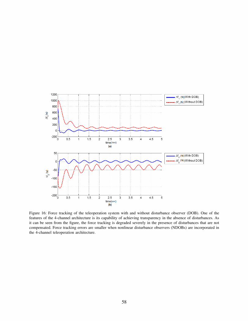
Figure 16: Force tracking of the teleoperation system with and without disturbance observer (DOB). One of thefeatures of the 4-channel architecture is its capability of achieving transparency in the absence of disturbances. Asit can be seen from the figure, the force tracking is degraded severely in the presence of disturbances that are notcompensated. Force tracking errors are smaller when nonlinear disturbance observers (NDOBs) are incorporated inthe 4-channel teleoperation architecture.

58

Figure 17: Disturbance tracking at the slave side in (a) x1 coordinate, and (b) x2 coordinate. It is assumed thatan external payload, with a mass equal to 0.5kg, is connected to the end-effector of the slave. Also, it is assumedthat a sinusoidal disturbance torque equal to τd = sin(4πt) is exerted to the second joint of the slave robot. Thedisturbance tracking errors at the slave side are uniformly ultimately bounded.

59

Figure 18: Disturbance tracking at the master side in (a) x1 coordinate, and (b) x2 coordinate. It is assumed thatan external payload, with a mass equal to 0.5kg, is connected to the end-effector of the slave. Also, it is assumedthat a sinusoidal disturbance torque equal to τd = sin(4πt) is exerted to the second joint of the slave robot. Thedisturbance tracking errors at the master side are uniformly ultimately bounded.

60

Sidebar 1: Brief Review of Nonlinear Systems

Uniform ultimate boundedness is a useful concept in nonlinear systems literature that can2

be effectively used for control design. This concept provides a practical notion of stability undercertain assumptions.4

Definition A solution of the nonlinear system x = f(t, x), x(t) : [t0,∞)→ Rn with initialcondition x(t0) = x0 is said to be uniformly ultimately bounded with respect to a set Ω if there6

exists a constant T ≥ 0, dependent on x0 and Ω, such that x(t) ∈ Ω for all t ≥ t0 + T .

In a closed-loop system, it is desired that the set Ω and the convergence time T depend on8

control parameters such that with proper design they can be made arbitrarily small. Moreover,if the domain of attraction can be arbitrarily enlarged by tuning control parameters, it is said10

that the closed-loop system is semi-globally practically stable. The following theorem gives asufficient condition for having the uniform ultimate boundedness property in terms of existence12

of a Lyapunov function.

Theorem 1 (Uniform Ultimate Boundedness): Let Br(0) be the open ball centered at the14

origin with radius r and V : Br0(0) × [0,∞) → Rn be a continuously differentiable functionsuch that16

c1|x|2 ≤ V (x, t) ≤ c2|x|2,∂V

∂xf(x, t) +

∂V

∂t≤ −c3|x|2, for all |x| ≥ µ > 0,

for all t ≥ 0 and all x ∈ Br(0). Take r0 > 0 such that r0 < r and µ < r0. Then, for every initialstate x(t0) ∈ Br0(0), the trajectories of the system converge with an exponential rate proportional18

to c3 to a ball centered at the origin with a radius proportional to 1c3

. Moreover, these trajectoriesenter the ball in a finite time T > 0 dependent on µ and x(t0), and remain within the ball after20

t0 + T .

The next theorem guarantees the existence of suitable Lyapunov functions when the system22

is exponentially stable.

Theorem 2 (Converse Lyapunov Theorem): Let x = 0 be an equilibrium point for the24

nonlinear system x = f(t, x), where f : [0,∞)× → Rn is continuously differentiable, Br(0) isthe open ball centered at the origin with radius r, and the Jacobian matrix [∂f

∂x] is bounded on26

Br(0), uniformly in t. Let k, λ, and r0 be positive constants with r0 < r/k. Let Br0(0) be theopen ball centered at the origin with radius r0. If the trajectories of the system satisfy28

61

|x(t)| ≤ k|x(t0)|e−λ(t−t0), for all x(t0) ∈ Br0(0), and all t ≥ t0 ≥ 0.

Then, there exists a function V : Br0(0)× [0,∞)→ Rn that satisfies the inequalities

c1|x|2 ≤ V (x, t) ≤ c2|x|2,∂V

∂xf(x, t) +

∂V

∂t≤ −c3|x|2,∣∣∣∣∂V∂x

∣∣∣∣ ≤ c4|x|,

for some positive constants c1, c2, c3, and c4.2

One of the fundamental concepts in analyzing the stability of nonlinear systems is thatof passivity. Passive systems, such as linear circuits that only contain positive resistors, possess4

desirable stability properties. Consider the nonlinear control affine system

x = f(x) + g(x)u,

y = h(x). (S1)

The system (S1) is said to be passive if there exists a nonnegative differentiable function, called6

the storage function, V with V (0) = 0 and nonnegative continuous function H with H(0) = 0

such that for all admissible inputs and initial conditions x(0) = x0 the following inequality8

holds:

V (x, u) ≤ yTu−H(x). (S2)

A weaker notion of passivity that is used in this article is that of quasi-passivity (or10

semi-passivity) that was first introduced in [S3] (see also [S4]). The system (S1) is said to semi-passive in D ⊂ Rn, if there exists a nonnegative function V : D → R+, D is open, connected12

and invariant under (S1) such that for all admissible inputs, for all initial conditions in D, andfor all time instants t for which the solutions of (S1) exist, the following inequality holds:14

V (x, u) ≤ yTu−H(x), (S3)

62

where the function H(x) is nonnegative outside the ball Br(0) ⊂ D for some positive constantr. If D = Rn, the system (S1) is called semi-passive.2

One of the properties of semi-passive systems is that these systems behave similar to passivesystems for large enough |x|. It can be shown that an output feedback of the form u = ξ(y)4

such that yT ξ(y) ≤ 0 makes the solutions of the semi-passive system ultimately bounded (see[S3], [S4] for more details).6

References

[S1] H. J. Marquez, Nonlinear Control Systems, Hoboken, NJ: John Wiley & Sons, Inc., 2003.8

[S2] M. W. Spong, S. Hutchinson, and M. Vidyasagar, Robot Modeling and Control, New York:Wiley, 2005.10

[S3] I. G. Polushin, “Stability results for quasidissipative systems”, in Proc. 3rd EuropeanControl Conf., Rome, Italy, 1995.12

[S4] I. G. Polushin, D. Hill, and A. L. Fradkov, “Strict quasipassivity and ultimate boundednessfor nonlinear control systems”, in Proc. 4th IFAC Symp. Nonlin. Cont. Syst. (NOLCOS),14

Enschede, The Netherlands, 1998, pp. 527–532.

63

Sidebar 2: PHANToM Omni and its Parameter Identification

The PHANToM Omni R© (Geomagic Inc., SC, USA) is a haptic device that can be employed2

in various applications such as virtual reality and teleoperation. The PHANToM Omni has threeactuated revolute joints which provide the user with force feedback information. In addition to4

the actuated joints, the PHANToM robot has three wrist joints that are passive.

The PHANToM dynamic model can be found in different sources (see, for example, [S5]).6

Defining ci = cos(qi), si = sin(qi), c2.i = cos(2qi), and s2.i = sin(2qi), the inertia matrix of thePHANToM robot, assuming q2 = 0, is given by [S5]:8

M(q) =

[α1 + α2c2.3 + α3s2.3 + α4c3 + α5s3 0

0 α6

], (S4)

and defining

V(q, q) = [V1, V2]T = C(q, q)q + G(q), (S5)

where the vector V(q, q) is the sum of the Coriolis, centrifugal and gravity forces, it is seen10

that

V1 = −2α2q1q3 sin(2q3) + 2α3q1q3 cos(2q3)

+α4q1q3 cos(q3)− α5q1q3 sin(q3),

V2 = 2α2q21 cos(q3) sin(q3)− α3q

21 cos(2q3)−

1

2α4q

21 cos(q3) +

1

2α5q

21 sin(q3)

+α7 sin(q3) + α8 cos(q3). (S6)

The Jacobian of the PHANToM, considering q2 = 0, is [S5]:12

J(q) =

[l1 + l2s3 0

0 l1s3

], (S7)

64

where l1 = l2 = 135mm are the lengths of the first and the second link of the robot. Therefore,the disturbance due to the external payload which is being exerted to the first and the third joints2

of the robot is:

τττ payload = JTF = JT

[0

mg

]=

[0

mgl1s3

]. (S8)

The PHANToM parameters can be identified in the absence of external payloads using4

the method proposed in [S7]. This method uses the dynamic equation of the PHANToM inthe linearly parameterized form (see Property P4 of EL systems)6

Y (q, q, q)α = τ, (S9)

where Y ∈ R2×8 is the regressor matrix and α = [α1, . . . , α8]T ∈ R8×1 is the vector of robotparameters to be identified. The expression for the PHANToM regressor matrix is [S5]8

YT =

q1 0

q1c2.3 − 2q1q3s2.3 2q21c3s3

q1s2.3 + 2q1q3c2.3 −q21c2.3

q1s3 + q1q3c3 −12q2

1c3

q1c3 − q1q3s312q2

1s3

0 q3

0 s3

0 c3

. (S10)

According to the method in [S7] and in order to avoid acceleration measurements, thedynamic model (S9) needs to be passed through a first order stable low-pass filter of the form10

ωLs+ωL

. In the parameter identification process, the cut-off frequency of the filter is chosen to be toequal to 8 Hz because this frequency is between noise frequencies and robot motion frequencies.12

After passing through the low-pass filter, the dynamic equation (S9) becomes

YL(q, q)α = τL, (S11)

65

TABLE S1: PHANToM Omni identified parameters: The PHANToM parameters can be identified in the absence ofexternal payloads using the method proposed in [S7]. This method uses the dynamic equation of the PHANToM inthe linearly parameterized form. In the identification process, the first and the third joints of the PHANToM wereunder PD (proportional-derivative) control and the second joint was locked at 0deg.

Parameter Value Parameter Valueα1 6.11× 10−3 ± 0.9× 10−3 α2 −2.89× 10−3 ± 0.43× 10−3

α3 −4.24× 10−3 ± 1.01× 10−3 α4 3.01× 10−3 ± 0.52× 10−3

α5 2.05× 10−3 ± 0.15× 10−3 α6 1.92× 10−3 ± 0.23× 10−3

α7 1.60× 10−1 ± 0.05× 10−1 α8 −8.32× 10−3 ± 2.78× 10−3

where YL is the filtered regressor matrix and τL is the filtered torque. A sum of 8 sinusoids, 4

sinusoids for each of the joints 1 and 3, with frequencies ranging from 0.2 Hz to 1 Hz were2

applied to the PHANToM to identify the 8 unknown parameters. For a persistent excitation oforder no less than 2n − 2, the sum of n sinusoids needs to be applied to an unknown plant4

for identification purposes [S8]. In the identification process, the first and the third joints of thePHANToM were under PD (proportional-derivative) control and the second joint was locked at6

0deg. The role of the simple position PD controller employed in the identification is to make therobot joints traverse persistently exciting trajectory profiles. In order to find the parameters of the8

PHANToM, the recursive least squares algorithm is employed [S6]. Following this procedure,the PHANToM parameters were identified; accordingly, Table S1 gives the PHANToM Omni10

identified parameters.

References12

[S5] E. Naerum, J. Cornella, and O. J. Elle, “Contact force estimation for backdrivable roboticmanipulators with coupled friction”, in Proc. IEEE Int. Conf. Intell. Robots Syst., Nice,14

France, pp. 3021-3027.[S6] K. J. Astrom and B. Wittenmark, Adatpive Control, Addison Wesley, 1995.16

[S7] B. Taati, A. M. Tahmasebi, and K. Hashtrudi-Zaad, “Experimental identification andanalysis of the dynamics of a PHANToM Premium 1.5A hatpic device”, Presence, vol.18

17, no. 4, pp. 327–342, 2008.[S8] T. Soderstrom and P. Stoica, System Identification, Prentice Hall, 1989.20

66

Sidebar 3: Brief Review of Euler-Lagrange Systems

The model of a fully actuated EL system with an N -dimensional configuration space2

Q = RN is given by

d

dt

∂L∂q− ∂L∂q

= τ, (S12)

where q ∈ Q is the vector of generalized coordinates, q ∈ TqQ = RN is vector of the generalized4

velocities, and τ ∈ RN is the vector of control inputs. The Lagrangian function L(q, q) : TQ =

R2N → R is a smooth function and assumed to have the form [S9]6

L(q, q) = T (q, q)− V(q), (S13)

where T (q, q) is the kinetic energy function and V(q) is the potential function which is assumedto be smooth and bounded from below.8

In the case of electrical networks, T (q, q) is the sum of the magnetic co-energies of theinductive elements in terms of the currents through the inductors, while V(q) is given by the10

sum of the electric field energies of the capacitive elements in terms of the charges on thecapacitors (see [S10] for further details). In the case of mechanical systems, T (q, q) is the sum12

of mechanical kinetic energies. We have T (q, q) = 12qTM(q)q where M(q) ∈ RN×N is the

generalized inertia matrix and is assumed to be symmetric and positive definite. The reader is14

referred to [S11] for the general case of Lagrangian systems with non-Euclidean configurationspaces.16

Substituting (S13) in (S12) yields

M(q)q +N(q, q) = τ + τd, (S14)

where,18

N(q, q) = C(q, q)q +G(q), (S15)

and C(q, q)q ∈ RN is the vector of Coriolis and centrifugal forces. Also, G(q) := ∂V∂q

are theforces generated by potential fields such as the gravitational field.20

67

Following the EL systems literature (see, for example, [S9]), it is assumed that the ELmodel under study has the following properties:2

P1

1) The inertia matrix M(q) satisfies4

ν1I ≤M(q) ≤ ν2I, (S16)

where ν1 and ν2 are some positive constants and Inequality (S16) holds uniformly withrespect to q.6

2) The matrix M(q) − 2C(q, q) is skew-symmetric; namely, zT[M(q) − 2C(q, q)

]z = 0 for

all z ∈ RN .8

3) The matrix C(q, q) is bounded in q and linear in q; namely,

C(q, q)z = C(q, z)q, (S17)∣∣C(q, q)∣∣ ≤ kc|q|, (S18)

for all z ∈ RN and some positive constant kc.10

4) Let qr ∈ Rn be an arbitrary vector. There exists a linear parameterization for EL modelsof the form M(q)qr +C(q, q)qr +G(q) = Υ(q, q, qr, qr)θ, where Υ is a regressor matrix of12

known functions and θ is a vector containing EL system parameters.

References14

[S9] R. Ortega, A. Lorıa, P. J. Nicklasson, and H. Sira-Ramırez, Passivity-based Control ofEuler-Lagrange Systems, Springer-Verlag, London, 1998.16

[S10] J. MA. Scherpen, D. Jeltsema, and J. B. Klaassens, “Lagrangian modeling of switchingelectrical networks”, Systems & Control Letters, vol. 48, no. 5, pp. 365–374, 2003.18

[S11] F. Bullo and A. D. Lewis, Geometric control of mechanical systems: modeling, analysis,and design for simple mechanical control systems, Springer Science & Business Media,20

2004.

68

Author Information

Alireza Mohammadi (alireza.mohammadi@mail.utoronto.ca) is currently a Ph.D. candidate2

in the Department of Electrical and Computer Engineering at the University of Toronto, Canada.He received the M.Sc. degree in Electrical and Computer Engineering from the University4

of Alberta, Canada in 2009. His research interests include robotic locomotion, medical andrehabilitation robotics, and nonlinear control theory.6

Horacio J. Marquez (hmarquez@ualberta.ca) received the B. Sc. degree from the InstitutoTecnologico de Buenos Aires (Argentina), and the M.Sc.E and Ph.D. degrees in electrical8

engineering from the University of New Brunswick, Fredericton, Canada, in 1987, 1990 and1993, respectively.10

From 1993 to 1996 he held visiting appointments at the Royal Roads Military College,and the University of Victoria, Victoria, British Columbia. In 1996 he joined the Department of12

Electrical and Computer Engineering, University of Alberta, as an Assistant Professor, becomingAssociate Professor in 2000, and Professor in 2003. From 2000 to 2004 he was Associate Chair of14

Graduate Studies, and from 2004 to 2014 he was Chair of Electrical and Computer Engineeringat the University of Alberta. His current research interest include nonlinear filtering and control,16

robust control, sampled-data systems, and control of cyber-physical systems. He is the Authorof Nonlinear Control Systems: Analysis and Design (Wiley, 2003).18

Dr. Marquez is a Licensed Professional Engineer (PEng) and a Fellow of the CanadianAcademy of Engineering (CAE), Fellow of the Engineering Institute of Canada (EIC), Fellow20

of the Institution of Engineering and Technology (EIT), and a Senior Member of the IEEE.

Mahdi Tavakoli (mahdi.tavakoli@ualberta.ca) is an Associate Professor in the Department22

of Electrical and Computer Engineering, University of Alberta, Canada. He received his BScand MSc degrees in Electrical Engineering from Ferdowsi University and K.N. Toosi University,24

Iran, in 1996 and 1999, respectively. He received his PhD degree in Electrical and ComputerEngineering from the University of Western Ontario, Canada, in 2005. In 2006, he was a26

post-doctoral researcher at Canadian Surgical Technologies and Advanced Robotics (CSTAR),Canada. In 2007-2008, he was an NSERC Post-Doctoral Fellow at Harvard University, USA. Dr.28

Tavakolis research interests broadly involve the areas of robotics and systems control. Specifically,his research focuses on haptics and teleoperation control, medical robotics, and image-guided30

surgery. Dr. Tavakoli is the lead author of Haptics for Teleoperated Surgical Robotic Systems(World Scientific, 2008).32

69