On nonlinear unknown input observers – applied to …folk.ntnu.no/torarnj/IJC_final2.pdf · On...

June 7, 2007 13:22 International Journal of Control paper˙final

International Journal of Control

Vol. 00, No. 00, DD Month 200x, 1–15

On nonlinear unknown input observers – applied to lateral vehicle velocity

estimation on banked roads

Lars Imsland∗,†, Tor Arne Johansen†,‡, Havard Fjær Grip†,‡, Thor Inge Fossen†,‡

†SINTEF ICT, N-7465 Trondheim, Norway‡NTNU, Department of Engineering Cybernetics, N-7491 Trondheim, Norway

(June 30th, 2006)

Unknown input observers (UIOs) are observers that have stable error dynamics that are independent of unknown inputs. This paperstudies such observers for nonlinear systems, and shows that the error dynamics for a nonlinear UIO has the same structure as the errordynamics of a nonlinear observer without unknown inputs. This result is first used to provide synthesis inequalities for UIOs for a classof nonlinear systems, and secondly, to inspire the design of an observer for estimation of vehicle lateral velocity on banked roads.

1 Introduction

Often, when estimating the state of state space models x = f(x) based on some measurements y = g(x) thatdepend on the states, one is faced with the presence of unknown inputs or disturbances in the differentialequations, x = f(x,w). A standard method in this case is to assume that some model of the parametertime variation is known (typically constant (w = 0), Markov models or Brownian motion in a stochasticsetting) and extend the state space model with this input model. Examples are the augmented extendedKalman filter (e.g. Gelb (1974)), or nonlinear observers with bias estimation (e.g. Vik and Fossen (2001)).

In this paper, another approach will be pursued, which does not assume known parameter dynamics,but rather relies on some geometric property of the system and output mapping. This property will allowus to specify observers that have error dynamics which are completely independent of the unknown input,denoted Unknown Input Observers (UIOs, see definition below). In the linear case, such observers are wellknown (e.g. Darouach et al. (1994), Chen et al. (1996)). For nonlinear systems, there exist some resultson UIOs, mostly in connection with fault detection and isolation, see, e.g., Seliger and Frank (1991). Ofmore recent results, we mention Rocha-Cozatl et al. (2004) who give conditions for design of UIOs basedon dissipativity, which for a special system class translate into LMIs (Rocha-Cozatl et al. 2005).

In this paper, we will give a simple extension of the results in the linear case to nonlinear systems. Thisextension is not reported in the literature, to the best of the authors’ knowledge, probably because it doesnot provide constructive design guidelines. In a similar manner as for linear systems in Darouach et al.(1994), which showed that finding a UIO for linear systems can be formulated as the problem of findinga (Luenberger) observer for a linear system, we show that (for a certain, fairly general class of nonlinearsystems) proving that a nonlinear UIO is stable is as hard as (but not structurally harder than) provingthat a nonlinear observer is stable in general.

Thereafter, using this result, we provide a synthesis procedure for nonlinear UIOs based on the observerdesign for a class of nonlinear systems described in Arcak and Kokotovic (2001).

Next, we show how the result inspire the re-design an observer for vehicle lateral velocity under theinfluence of road bank angle. This problem has to some extent been studied earlier in the context of vehicledynamics control systems, for example using an augmented EKF (Suissa et al. 1994), using linear observersaugmented with road bank angle estimation (Fukada 1999), estimating road bank angle separately fromlateral velocity (Tseng 2001, Ungoren et al. 2004), or using additional measurements such as DGPS (Hahn

∗Corresponding author. Email: [email protected].


2 On nonlinear unknown input observers

et al. 2004). Linear UIO methods were used in Liu and Peng (2002). Our approach extends the resultsin Imsland et al. (2006) to banked roads, and differs from earlier approaches since we use a nonlinearfriction model and analyze stability of the observer error dynamics. In addition to directly applying thenonlinear UIO theory, we also propose a method that estimates the unknown input. This observer is testedon real vehicle data.

The following definition of Unknown Input Observers is adapted from Moreno (2000) (with abuse ofnotation and some standard technicalities left out for brevity):

Definition 1.1 Given the (possibly) nonlinear system x = f(x, u,w), y = h(x, u), with x the state, uknown input, w unknown input and y measured output. The system (the observer)

z = φ(z, u, y),

x = ξ(z, u, y),

is an unknown input observer (for the above system) if

limt→∞

‖x(t) − x(t)‖ = 0,

uniformly in (that is, the rate of convergence is independent of) t0 and w(·) (and initial conditions).

One technicality required is that solutions to the nonlinear system to be observed must exist for all futuretime. This is implicitly assumed (including the necessary smoothness-assumptions on f and h) throughoutthe paper.

2 Linear systems

This section reviews some results on UIOs for linear systems.

2.1 UIOs for linear systems

Consider the LTI system

x = Ax + Bu + Dw, y = Cx, (1)

where x, u and w are the state, the known inputs and the unknown inputs, respectively, while y is the(measured) output. It is generally acknowledged (e.g. Darouach et al. (1994), Chen et al. (1996)) that fullorder UIOs for linear systems take the (Luenberger observer-like) form

z = Nz + Ly + Gu, x = z − Ey. (2)

The matrices N , L, G and E must be specified such that the dynamics for the observer error x = x − xcan be written ˙x = Nx, where N is Hurwitz. Then, the error system is (globally) exponentially stable andindependent of the unknown input w, and hence the observer is a UIO according to Definition 1.1.


On nonlinear unknown input observers 3

By constructive design, the following matrix equalities give a UIO1:

(I + EC)D = 0, (3a)

G = (I + EC)B, (3b)

N = (I + EC)A − L1C, (3c)

L = −NE + L1. (3d)

The existence conditions for solutions (for N (stable), L, G and E) are that rankCD = rankD = dim y,and that the pair ((I + EC)A,C) is detectable (Darouach et al. 1994, Chen et al. 1996). The crucialidentity to solve is (3a), which under the existence conditions is solved (for E) as

E = −D(CD)+ + Y (I − CD(CD)+), (4)

where (CD)+ is the left inverse of CD, (CD)+ = [(CD)TCD]−1(CD)T, and Y is an arbitrary matrix ofappropriate dimensions. It is this operator that “decouples” the unknown input.

It is interesting to write the observer in terms of a differential equation for x:

˙x = z − Ey

= N(x + Ey) + LCx + Gu − EC(Ax + Bu + Dw)

= (I + EC)Ax − L1Cx + NEy − NECx + L1Cx + (I + EC)Bu − EC(Ax + Bu + Dw)

= Ax + Bu + L1(Cx − Cx) + EC(Ax + Bu) − EC(Ax + Bu + Dw).

Since (I + EC)D = 0, the term Dw can be moved out from the last paranthesis, thus we can write this as

˙x = Ax + Bu + Dw + L1(y − Cx) − ECA(x − x).

This is essential, since the term Dw then disappears from the error dynamics,

˙x = x − ˙x

= Ax + Bu + Dw − Ax − Bu − Dw − L1(y − Cx) + ECA(x − x)

= Ax − L1Cx + ECAx

= Nx.

For stability, L1 (and Y ) must be chosen such that N is Hurwitz, which is always possible under thedetectability assumption mentioned above. If we strengthen the assumption to observability of ((I +EC)A,C), we see that the eigenvalues of N can be placed arbitrarily. A procedure for constructing linearUIOs can be summarized as a) calculate E using (4), b) find L1 such that N = (I + EC)A − L1C isHurwitz, and c) calculate G (3b) and L (3d).

If we consider the case with dim y = dimw = 1, existence of an UIO requires relative degree (w.r.t. w)equal to one, since we must have CD 6= 0 for (3a) to be solvable. In higher dimensions we see from (4)that we must have CD left invertible, which for dimw = 1 means that at least one measurement mustdepend directly on one of the states that w affects.

Finally, we stress again that the property (3a) factors out Dw from the error dynamics, since

Ey = ECx = EC(Ax + Bu) + ECDw = EC(Ax + Bu) − Dw.

1Eliminating L1, the two last equations can be written as N = (I + EC)A − LC − NEC, which gives the same conditions as Darouachet al. (1994).



2.2 Disturbance observers for linear systems

The above observer can be expanded to also provide an estimate of the disturbance d = Dw. Consider theestimate (very similar to what is proposed in Liu and Peng (2002)),

d = L1y − Ey − (L1C − ECA)x + ECBu.

Then,

Dw − d = Dw − L1y + EC(Ax + Bu + Dw) + (L1C − ECA)x − ECBu

= (I + EC)Dw − (L1C − ECA)x

= −(L1C − ECA)x.

Since x → 0, we conclude that d → Dw. Furthermore, if D is full row rank (and dim d ≤ dimx), w can befound from d.

It is noteworthy that the convergence of the estimate d to Dw is completely independent of w. Aconsiderable practical disadvantage of this approach is that the estimate depends on the differentiatedoutput, y.

3 UIO for nonlinear systems

In this section, we use insights from the previous section to specify conditions for nonlinear UIOs.First, note that if only nonlinearities that depend on known signals (inputs and outputs, i.e. of the form

γ(y, u)) appear in the system dynamics, the same procedure as for linear UIOs gives a nonlinear UIO, assuch nonlinearities can be canceled in the error dynamics. This section treats general nonlinearities thatdepend on unmeasured states, but for illustration, we have included a nonlinearity of the form γ(y, u) inthe design procedure in Section 4.

3.1 Linear measurement equation

Consider the nonlinear system

x = f(x, u) + Dw, y = Cx. (5)

A nonlinear UIO for this system with structure1 as in the LTI case, is

z = (I + EC)f(z − Ey, u) + L1(y − C(z − Ey)), x = z − Ey. (6)

Assuming (I + EC)D = 0, it is easy to see that we can write

˙x = f(x, u) + Dw + L1(y − Cx) − EC (f(x, u) − f(x, u)) .

This gives the following observer error system:

˙x = (I + EC)(f(x, u) − f(x, u)) − L1(y − Cx),

which is independent of w.From the above, we conclude the following theorem:

1Replacing f(x, u) with Ax + Bu and using (3), we get (2).



Theorem 3.1 Assume that rankCD = rankD = dim y for (5), and let the constant matrix E be givenby (4). Then the system (6) is a nonlinear UIO for (5) if the constant matrices Y and L1 are chosen suchthat x = 0 is a uniformly globally asymptotically stable equilibrium of the system

˙x = (I + EC)(f(x, u) − f(x − x, u)) − L1Cx.

Thus, as long as the rank-assumption holds, designing L1 to get a UGAS error system is in principleas hard as (but not harder than) designing a UGAS observer with linear injection term in general. Thecorresponding conclusion was made for linear UIOs in Darouach et al. (1994).

3.2 Nonlinear measurement equation

Assume now that the system is given by

x = f(x, u) + Dw, y = h(x). (7)

Since the measurement equation is not linear, we cannot apply (3a) directly, as we did in the previoussection. Replacing the linear mapping E with a nonlinear mapping e(y), we propose the following structurefor the nonlinear UIO:

z = g(z, y, u), x = z − e(y).

where the nonlinear functions g(z, y, u) and e(y) are to be found. We do not consider measurement equa-tions that depends on the input, h(x, u) (or a mapping e(y, u) instead of e(y)), since this will result innonlinear UIOs that depend on the time derivative of the inputs.

Proceeding as in the previous section, it is easy to show that if we can find e(y) such that, similar to (3a),

(

I +∂e

∂y

∂h

∂x

)

D = 0, ∀x, (8)

then we can design a UIO. The natural choice for g is then

g(z, y, u) =

(

I +∂e

∂y

∂h

∂x

)

f(z − e(y), u) + L1(y − h(z − e(y))).

We see that such an observer is only possible if ∂e∂y

∂h∂x

is independent of x, which in general is hard to

obtain. However, in some cases, the structure of e(y) can be chosen such that this condition holds, forexample if one has a mixture of linear and nonlinear measurements. Then the linear measurements canbe used to decouple the unknown input, while the nonlinear (and linear) measurements can be used tostabilize the error dynamics.

As an example, consider the system

x = f(x, u) + Dw, y =(

yT

1 , yT

2

)T

=(

(Cx)T, h(x)T)T

.

For this system, we propose the UIO

z = (I + EC)f(z − Ey1, u) + L1(y1 − C(z − Ey1)) + L2(y2 − h(z − Ey1)), x = z − Ey1. (9)

Proceeding as in Section 3.1, if we can find E such that (I + EC)D = 0, then the observer error dynamicscan be written

˙x = (I + EC)((f(x, u) − f(x − x, u)) − L1Cx − L2(h(x) − h(x − x)),



which is independent of the unknown input w. Notably, we can use all measurements (both L1 and L2)to stabilize the error dynamics, while only the linear measurement y1 is used to make the observer errorindependent of w.

3.3 Toward constructive design

As mentioned above, the previous sections give conditions for an observer to be a nonlinear UIO, and donot give constructive guidelines. However, there exist in the literature some design procedures for nonlinearobservers, which by Theorem 3.1 can also be used for design of nonlinear UIOs. Most notably, perhaps, arethe results of Arcak and Kokotovic (2001), Fan and Arcak (2003), which we combine with Theorem 3.1 inthe next section.

Observer design procedures for a certain class of output nonlinearities can be found in Fan and Arcak(2003). These can be combined with the results in Section 3.2, but as the combination is similar to thenext section, we do not go into detail on this.

In Section 5, we will look at how we can apply the insights gained in this section to the problem ofestimating lateral velocity of cars on banked roads.

4 Nonlinear UIOs based on circle criteria observers

Consider now nonlinear systems on the form

x = Ax + Gρ(Hx) + γ(y, u) + Dw, y = Cx, (10)

where the first nonlinearity ρ : Rp → R

p satisfies a monotonicity property to be specified.We will use the results in Arcak and Kokotovic (2001), Fan and Arcak (2003) to define synthesis in-

equalities which upon feasibility gives observer injection gains which stabilize the observer error dynamicsof Theorem 3.1.

4.1 Observer and synthesis inequality

We propose the following observer for (10):

z = (I + EC)A(z − Ey) + (I + EC)Gρ (H(z − Ey) + K(y − C(z − Ey)))

+ L1(y − C(z − Ey)) + (I + EC)γ(y, u), x = z − Ey, (11)

where E is given by (4) such that (I + EC)D = 0. A slight change is made compared to the previoussection, we use an additional injection gain K, following the approach of Arcak and Kokotovic (2001).Differentiating the estimated state gives

˙x = Ax + Gρ(Hx + K(y − Cx)) + γ(y, u) + Dw

− ECA(x − x) − ECG (ρ(Hx) − ρ(Hx + K(y − Cx))) + L1(y − Cx).

This gives the following observer error system, independent of w:

˙x = (I + EC)Ax + (I + EC)G (ρ(Hx) − ρ(Hx + KCx)) − L1Cx. (12)

If we define

φ(v, ζ) = ρ(v) − ρ(v − ζ), v := Hx,



the error system (12) can be rewritten as

˙x = ((I + EC)A − L1C) x + (I + EC)Gφ(v, ζ), ζ = (H − KC)x.

Assumption 4.1 The function ρ(v) satisfies the monotonicity property

∂ρ

∂v+

(

∂ρ

∂v

)

T

≥ 0, ∀v ∈ Rp.

This assumption implies that φ(v, ζ) satisfies the sector property ζTφ(v, ζ) ≥ 0, and this allows toconclude asymptotic stability if the linear system with input −φ(v, ζ) and output ζ is strictly positive real(SPR), which is implied by the existence of P > 0 and a constant κ > 0 such that

(

((I + EC)A − L1C)T P + P ((I + EC)A − L1C) + κI P (I + EC)G + (H − KC)T

GT(I + EC)TP + (H − KC) 0

)

≤ 0. (13)

This inequality is a linear matrix inequality (LMI) in P , PL1, K, and κ. Since P > 0, L1 can be obtainedfrom PL1.

Theorem 4.2 If observer injection gains L1 and K, matrices P > 0 and κ > 0 exist such that (13) isfeasible, then the observer (11) is a UIO, whose error dynamics are UGES.

Proof [Outline] The proof follows by checking that the SPR condition guarantees that the derivative ofthe Lyapunov function V (x) = xTPx is negative definite along the trajectories of (12), implying thatthe origin of the observer error dynamics, which by design are independent of the unknown input w, areuniformly globally exponentially stable (and thus uniformly convergent). �

Remark 1 In Fan and Arcak (2003), the observer design in Arcak and Kokotovic (2001) is extended in twodirections. The same can be done for the design in this section. First, if it is possible to find a structuredmultiplier matrix Λ such that (Λζ)Tφ(v, ζ) ≥ 0 for all Λ > 0 with this particular structure, then thestructured matrix Λ can be used to generalize (13). This applies if the multivariable nonlinearity ρ(v) hasa decoupled structure.

Moreover, synthesis inequalities for the system class (10) with additional (monotone) output nonlinear-ities are also specified. This design can be combined with the approach in Section 3.2 to give synthesisinequalities for existence of a UIO. As the procedure is similar to that above, the details are not givenhere.

Remark 2 Rocha-Cozatl et al. (2005) develops a synthesis SDP for nonlinear UIOs for essentially the sameclass of system that is considered in this section. Although both the approach herein and the approachof Rocha-Cozatl et al. (2005) is based on dissipativity and result in LMIs, the synthesis inequalities havedifferent structure and it is not straightforward, for a given problem, to say whether one approach is lessconservative than the other. However, the approach in Rocha-Cozatl et al. (2005) is more general in thesense that several types of dissipativity can be exploited, while the approach herein is simpler; it has feweroptimization variables, and is a more direct extension of linear UIO design, since it uses the property (3a).

4.2 Example using circle criteria design

Consider the mass-damper system taken from Rocha-Cozatl et al. (2005),

x =

0 1 0 0

−k1+k2

m1

− b1+b2m1

k2

m1

b2m1

0 0 0 1k2

m2

b2m2

− k2

m2

− b2m2

x +

01

m1

00

u +

0− 1

m1

00

ρ (x2) +

0001

m2

w



where we measure x1 and x4, and the nonlinearity ρ is due to a nonlinear damping device, ρ(v) =cnl sign(v) ln(1 + |v|). This system is of the class (10), and since dρ/dv > 0 always, Assumption 4.1 holds.The aim of this example is to illustrate the UIO design in Theorem 4.2, by designing a UIO for estimatingthe unmeasured state variables x2 and x3. Parameter values can be found in Rocha-Cozatl et al. (2005).

Using LMI solvers in Yalmip (Lofberg 2004), we find that the output injections

L1 =

−0.3501 0.7234−4.5838 −0.23510.2936 1.4022−0.8632 0.5000

, K =(

−0.8780 0)

,

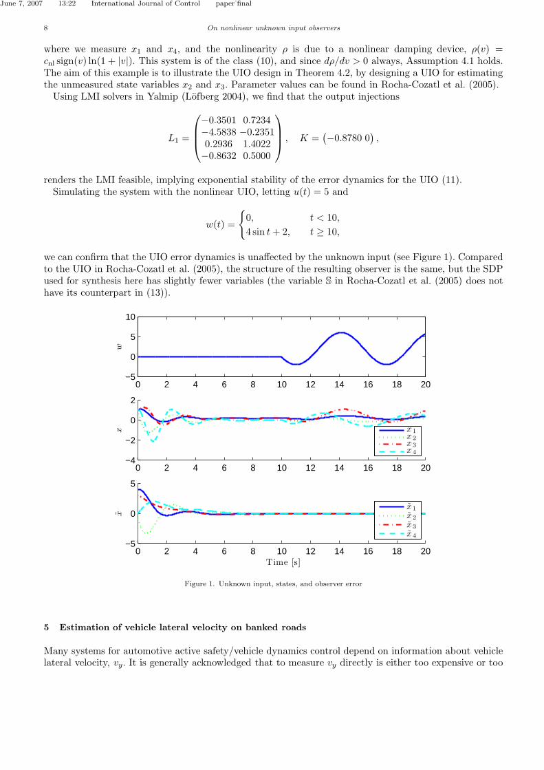
renders the LMI feasible, implying exponential stability of the error dynamics for the UIO (11).Simulating the system with the nonlinear UIO, letting u(t) = 5 and

w(t) =

{

0, t < 10,

4 sin t + 2, t ≥ 10,

we can confirm that the UIO error dynamics is unaffected by the unknown input (see Figure 1). Comparedto the UIO in Rocha-Cozatl et al. (2005), the structure of the resulting observer is the same, but the SDPused for synthesis here has slightly fewer variables (the variable S in Rocha-Cozatl et al. (2005) does nothave its counterpart in (13)).

0 2 4 6 8 10 12 14 16 18 20−5

0

5

10

w

0 2 4 6 8 10 12 14 16 18 20−4

−2

0

2

x

x1

x2

x3

x4

0 2 4 6 8 10 12 14 16 18 20−5

0

5

Time [s]

x

x1

x2

x3

x4

Figure 1. Unknown input, states, and observer error

5 Estimation of vehicle lateral velocity on banked roads

Many systems for automotive active safety/vehicle dynamics control depend on information about vehiclelateral velocity, vy. It is generally acknowledged that to measure vy directly is either too expensive or too



unreliable; thus some kind of estimation algorithm, or observer, must be used. The standard measurementsuite used for obtaining an estimate of vy consists of wheel speed measurements ωi (which can be used tocalculate an estimate of longitudinal velocity vx), steering wheel angle δ (used to calculate individual wheelangles δi), yaw rate r and lateral acceleration ay. All these measurements can be considered standard inmodern cars with yaw stabilization (anti-skid) systems, such as the Bosch ESP system (van Zanten 2000).The acceleration and yaw rate measurement are typically obtained from MEMS-based sensors which weassume is located in the center of gravity (or corrected if this is not the case), and to have bias and slow driftcomponents removed by appropriate filtering. Observers for vy can be found in the literature, e.g. (Kienckeand Nielsen 2000, Imsland et al. 2006), and are also implemented in production cars (van Zanten 2000).However, except for the Extended Kalman Filter (EKF) (Suissa et al. 1994), the authors are not awareof any approaches reported in the literature that use nonlinear techniques (models) for estimating lateralvelocity taking banked roads explicitly into account. The main advantage of the approach herein comparedto using EKF-based designs is lower computational complexity, since there is no Riccati equation to besolved online.

φ

yin

zCG

yUC

φR

yCG

zin

UC

CG

RC

zUC

Figure 2. Vehicle seen from behind, illustrating the road bank angle and the different coordinate systems involved. The abbrieviationsCG, RC and UC stands for center of gravity, roll center and undercarriage (center), respectively. Subscript in denotes an inertial frame.

In this paper we assume that the roll angle φ is zero (or known, such that correction is possible).

Only ay of the above mentioned measurements depends algebraically on vy. This dependence is givenby a force balance in the lateral direction of the vehicle, resulting in

ay =1

mfy(vy, u), (14)

where fy is based on a highly nonlinear road/tire friction model and u contains the other known vari-ables/measurements that enter the friction model (see, e.g., Pacejka (2002)). We have here disregardedvehicle roll, and assumed that ay is the sensor reading of a sensor attached to the vehicle body, alignedwith a coordinate system placed in the center of gravity, see Figure 2. This last assumption means that ay

will be different from the actual ay when there is a non-zero road bank angle (or vehicle roll).The dynamic equation for vy (assuming the vehicle is a rigid body, and ignoring roll and pitch motion)

is

vy = −vxr + ay − g sin φR, (15)

where the term vxr is the rotational term (longitudinal velocity multiplied with yaw rate) stemming fromthe vehicle body frame being accelerated with respect to the inertial frame. The last term, g sin φR isnon-zero if the road is banked, φR being the bank angle (see Figure 2) and g the acceleration of gravity.This term can be considered an unmeasured/unknown input (w = g sin φR), and we want to design a(nonlinear) observer for vy that is robust to non-zero w. This is a challenging problem, see for examplethe discussion in van Zanten (2000).

For horizontal vehicle models such as (15), and also the bicycle model or the two-track model (Kienckeand Nielsen 2000), any UIO must make use of the ay measurement. This is because the road bank angle



only affects the vy state, that is, for the model class in Section 3, the only non-zero element of D is

the element corresponding to vy. From (8) we see that we must have ∂e∂y

∂h∂x

D 6= 0 for a measurement

equation h(x) (the arguments remain the same if h depends on u). This means that we must have ∂h∂vy

6= 0.

Considering the measurements mentioned above, ay is the only measurement that depends on vy and thush must contain ay. See also the discussion at the end of Section 2.1.

5.1 Nonlinear unknown input observer for vehicle lateral velocity on banked roads

The direct application of the methods in Section 3.2 would lead to an observer that depends on the time-derivative of u, since u appears in the measurement equation (14). This is not desirable, and hence wedo not pursue this path. Therefore, we investigate whether it is possible to obtain a linear measurementequation and thus be able to use an observer of the form (6). For this, we must invert the measurementequation (14),

vcy = f−1

y (ay, u),

where we use vcy to distinguish the vy calculated based on measurements from the real state vy. This

inversion generally requires numerical methods, or we can use an approximation based on a first orderTaylor expansion of fy,

vcy = f−1

y (ay, u) ≈

(

∂fy(vy, u)

∂vy

)

−1 (

may − fy(vy, u) +∂fy(vy, u)

∂vyvy

)

, (16)

where vy is an estimate of vy, and the closer vy is to vy, the better the approximation is. Designing aUIO based on this calculated measurement using the results in Section 3.1, we find that we must chooseE = −1, and get

z = −Lz, vy = z + vcy.

The last equation is implicit in vy if using (16), but this can in principle be solved using standard numericaltechniques. However, we see that this observer is nonsensical, z will converge to zero and the estimate willbe vc

y, without any filtration. If we use (9) with y1 = vcy and y2 = ay instead, we end up with the following

UIO observer:

z = −L1z + L2

(

ay −1

mfy(vy, u)

)

, vy = z + vcy. (17)

Under the assumption that ∂fy/∂vy has constant sign (see Assumption 5.1 in the next section), it isstraightforward to show that this observer is convergent for any L1 ≥ 0, and L2 > 0. However, thisobserver does not use the dynamic model for vy, since both parts of the observer (z and vc

y) depend merelyon the friction model. This has two drawbacks:

• Measurement noise: All measurement noise (and other measurement errors) will affect the vy estimatedirectly. To a certain degree, this problem can be rectified by filtering the estimate. However, betterfiltering can be obtained by using the dynamic model.

• Measurement model errors: The friction model will contain errors due to assumptions made in specifyingthe model, tear and wear of tyres, and varying road surfaces. Moreover, for large side-slips, it is practicallyimpossible to invert the friction model, since nonlinear friction models become almost flat with respectto variations in lateral velocity (∂fy/∂vy ≈ 0, cf. (16)). The observer (17) has limited possibilities fordetuning weight on use of the friction model in such situations.

Therefore, we develop a slightly different observer for this problem, which will not be a UIO by definition,but it is an extension of the observer in Imsland et al. (2006) inspired by the UIO design, taking the above



weaknesses into account.

5.2 Observer with estimation of road bank angle

Due to the weaknesses of the pure UIO design, we use the UIO observer (17) together with the observerfrom Imsland et al. (2006), by including an estimate of w = g sin φR:

˙vy = −vxr + ay − w − Kvy(ay −

1

mfy(vy, u)), (18a)

z = −Kvy

(

ay −1

mfy(vy, u)

)

, ν = z + vcy, (18b)

w = Kw(vy − ν). (18c)

We have, for simplicity, chosen L1 = 0, and used L2 = Kvyfor correspondence with the notation in Imsland

et al. (2006). Compared to the unknown input observer in the previous section, this observer does makeuse of the dynamic model for vy, and additionally makes it possible to tune down the effect of w on the vy

estimate in periods when we know w is inaccurate (that is, in periods when the friction model is inaccurateor not invertible due to for example high slips). Another significant practical advantage over (17), is thatuse of approximations such as (16) do not result in an implicit equation for vy that in practice must besolved by iteration.

On the other hand, (18) is not a UIO, since the convergence of vy is not independent of w. Its design is,however, strongly inspired by the UIO design (17) that leads to (18b).

This observer is globally convergent under the following two assumptions:

Assumption 5.1 The friction model is continuously differentiable in its arguments, and there exists aconstant c > 0 such that the following holds globally:

∂fy(vy, u)

∂vy≤ −c.

Assumption 5.2 The road bank angle is constant, φR = 0.

Assumption 5.1 is realistic, although there may exist combinations of tire models and large slips for whichit does not hold on short time intervals, see discussion in Imsland et al. (2006). The second assumptiondoes not hold in general, but it is nevertheless a standard type of assumption in many parameter adaptivestate estimation schemes. If the road bank angle changes slowly or rarely, the assumption may be justified.It is notable that this assumption was not needed in the pure UIO design.

Define the observer errors as vy := vy − vy, and w := w − w = w + Kw (z + vy). The observer errordynamics can then be written, using Assumption 5.2,

˙vy = −w + Kvy

(

ay −1

mfy(vy, u)

)

, (19a)

˙w = −Kww. (19b)

Theorem 5.3 If the observer gains are chosen such that KvyKw > 1

4mc, the origin of the observer error

dynamics (19) is uniformly globally exponentially stable (UGES).



Proof Consider the Lyapunov function candidate V = 12(v2

y + w2). We have

V = vy

(

−w + Kvy(ay −

1

mfy(vy, u))

)

− Kww2

= vyKvy(ay −

1

mfy(vy, u)) − vyw − Kww2

y

≤ −mcKvyv2y − vyw − Kww2

y,

where we have used Assumption 5.1 and the Mean Value Theorem. The right-hand-side expression canbe made negative definite by choosing Kvy

> 0 and Kw > 0 such that KvyKw > 1

4mc, and thus V is a

Lyapunov function for (19) showing exponential stability (e.g. Khalil (2002)). �

Remark 1 The observer (18) can be extended with yaw rate and longitudinal velocity as estimated states,using a straightforward combination of the above results and those of Imsland et al. (2006).

Remark 2 Note that the above observer is a disturbance observer, which does not depend on time-derivatives of inputs or outputs. The linear disturbance observer in Section 2.2 depends on the time-derivatives of the output, and, in general, this would also be the case if one were to use the same techniquesfor the class of nonlinear system in Section 3.1. Because of the structure of the problem, this can be avoidedin the above design.

Remark 3 One might use vcy directly to calculate w = vc

y − ay + vxr, to insert in (18a). In doing this,however, one does not use feedback from ay and the friction model to correct errors in vc

y, that is, onelooses a robustifying feedback path.

5.3 Experimental results from real vehicle measurements

The real vehicle data are from a (dry concrete surface) test track with straight flat sections and steepbanked curves. In the data set illustrated in Figure 3, the car first drives straight, then takes a turn on abanked curve before driving in a slalom pattern on flat ground. As can be seen from the figure, we obtainreasonably good estimates of vehicle velocity. Compared to the estimator without bank angle compensation((18a) with w = 0), the velocity estimate is considerably improved during the banked turn. For illustrationof the scenario, the individual wheel lateral tire slips are shown in Figure

The estimate of the road bank angle is not very accurate, especially during the slalom driving pattern.The main reasons are model errors, especially due to high side slips during the slalom (discussed below),and roll motion. This vehicle is a relatively large vehicle which exhibits significant roll motion duringturning. The effect of roll angle will enter additively to the road bank angle in (15). There is a trade-offhere: Tuning down Kw reduces the influence of these errors, but it also increases estimation error whenthere is non-zero road bank angle.

5.4 Discussion of lateral velocity observer

When estimating both vy and φR using the measurements explained above, we have two unknowns in-volved in one dynamic equation (15), and one measurement that depends algebraically on only one of theunknowns (14). Thus, it follows that in estimating both of them, one needs to fully exploit the measure-ment equation (the friction model). One could argue that adding the dynamic model as in the observer inSection 5.2 does not help, since one is actually adding another unknown (the road bank angle) at the sametime. However, it does help if one in addition has information about the dynamics of φR (for example thatit is slowly varying), and other information about the quality of the estimate.



0 10 20 30 40 50 60−2

−1

0

1

2

vy

[m/s]

0 10 20 30 40 50 60−20

−10

0

10

20

φR

[o]

T ime [s]

Figure 3. Top: Measured vy (whole), estimated vy with bank angle compensation (dashed) and estimated vy without bank anglecompensation (dotted). Bottom: Estimate of road bank angle. We have used Kvy

= 1 and Kw = 8.

0 10 20 30 40 50 60

−0.1

0

0.1

Time [s]

αi[o

]

Figure 4. Individual wheel tire slip angles αi, i = 1, . . . , 4. Whole line is front left, dashed line front right, dotted line rear left, anddash-dotted line rear right (the two rear slip angles are nearly identical).

For example, a problem with the inversion in (16), is that the partial derivative

1

m

∂fy(vy, u)

∂vy(20)

may become very small for maneuvers with large side slips, implying that the inverse in (16) becomeslarge, leading to high gain on a noisy measurement. A possible remedy is to try to recognize this situationand take corrective steps. However, situations where this happen are rather rare and brief, and in mostcases, one will drive (also on banked roads) with limited side slips. In the observer used in Figure 3, weset Kw = 0 and let w approach zero when the estimated partial derivative is below a certain limit. This


14 REFERENCES

happens for brief intervals during the slalom-part.If one uses linear friction models, as in Liu and Peng (2002), the partial derivative (20) will never become

small, but the problem remains due to large model errors for large side-slips.An important parameter in the friction model, the maximum friction coefficient, is known to vary

significantly with road conditions. Real-time knowledge of this parameter is therefore important for theobserver proposed in the previous section to work. (Grip et al. 2006, 2007) has extended the observerin Imsland et al. (2006) with adaptation of the friction parameter, and our overall goal is to obtainan observer which estimates lateral velocity robustly, subject to different road conditions and road bankangles. As discussed in van Zanten (2000), in some situations it is very hard to distinguish between changesin road bank angle and changes in friction, and hence it may be sensible to only estimate one of them atany given time, using suitable logic.

The complete velocity observer from Imsland et al. (2006), extended with friction adaptation from Gripet al. (2006, 2007) and road bank angle adaptation using the techniques developed here, is implemented,validated and compared to an EKF in Imsland et al. (2007). The results there show that the performanceof the nonlinear approach is at least as good as the performance of the EKF, with significantly lowercomputational complexity.

6 Concluding remarks

A simple observation on the error dynamics of nonlinear unknown input observers has been presentedin Theorem 3.1. This observation was first used to specify synthesis inequalities for a class of nonlinearsystems with unknown inputs, and then applied to a challenging problem in the automotive industry:Estimation of vehicle lateral velocity on banked roads. The pure UIO approach to this problem proved tohave some practical disadvantages, and we therefore, inspired by the UIO design, proposed an approachwhich better exploits both the dynamic model and the measurement equation.

Acknowledgments

We gratefully acknowledge DaimlerChrysler (Dr. Jens C. Kalkkuhl and Mr. Avshalom Suissa) for discus-sions and for supplying measurement series and vehicle data for the results in Section 5.1. The research issupported by the European Commission STREP project CEmACS, contract 004175.

References

Arcak, M. and Kokotovic, P.: 2001, Nonlinear observers: A circle criterion design and robustness analysis,Automatica 37(12), 1923–1930.

Chen, J., Patton, R. J. and Zhang, H.-Y.: 1996, Design of unknown input observers and robust faultdetection filters, International Journal of Control 63(1), 85–105.

Darouach, M., Zasadzinski, M. and Xu, S. J.: 1994, Full-order observers for linear systems with unknowninputs, IEEE Transactions on Automatic Control 39(3), 606–609.

Fan, X. and Arcak, M.: 2003, Observer design for systems with multivariable monotone nonlinearities,Systems & Control Letters 50(4), 319–330.

Fukada, Y.: 1999, Slip-angle estimation for stability control, Vehicle Systems Dynamics 32, 375–388.Gelb, A. (ed.): 1974, Applied optimal estimation, The MIT Press, Cambridge, Mass.-London. Written

by the technical staff of The Analytic Sciences Corporation, Principal authors: Arthur Gelb, Joseph F.Kasper, Jr., Raymond A. Nash, Jr., Charles F. Price and Arthur A. Sutherland, Jr.

Grip, H. F., Imsland, L., Johansen, T. A., Fossen, T. I., Kalkkuhl, J. C. and Suissa, A.: 2006, Nonlinearvehicle velocity observer with road-tire friction adaptation, Proc. 45th IEEE Conf. Decision Contr., SanDiego.


REFERENCES 15

Grip, H. F., Imsland, L., Johansen, T. A., Fossen, T. I., Kalkkuhl, J. C. and Suissa, A.: 2007, Nonlinearvehicle side-slip estimation with friction adaptation, Automatica . Accepted.

Hahn, J.-O., Rajamani, R., You, S.-H. and Lee, K. I.: 2004, Real time identification of road-bank angleusing differential GPS, IEEE Transactions on Control Systems Technology 12(4), 589–599.

Imsland, L., Grip, H. F., Johansen, T. A., Fossen, T. I., Kalkkuhl, J. C. and Suissa, A.: 2007, Nonlinearobserver for lateral velocity with friction and road bank adaptation – validation and comparison withan extended kalman filter, Proc. SAE World Congress.

Imsland, L., Johansen, T. A., Fossen, T. I., Grip, H. F., Kalkkuhl, J. and Suissa, A.: 2006, Vehicle velocityestimation using nonlinear observers, Automatica 42(12), 2091–2103.

Khalil, H. K.: 2002, Nonlinear Systems, 3rd edn, Prentice Hall, Upper Saddle River, NJ.Kiencke, U. and Nielsen, L.: 2000, Automotive Control Systems, Springer.Liu, C.-S. and Peng, H.: 2002, Inverse-dynamics based state and disturbance observers for linear time-

invariant systems, Journal of Dynamic Systems, Measurement, and Control 124, 375.Lofberg, J.: 2004, YALMIP : A toolbox for modeling and optimization in MAT-

LAB, Proceedings of the CACSD Conference, Taipei, Taiwan. Available fromhttp://control.ee.ethz.ch/~joloef/yalmip.php.

Moreno, J.: 2000, Unknown input observers for SISO nonlinear systems, Proceedings of the 39th IEEEConference on Decision and Control, Sydney, Australia.

Pacejka, H. B.: 2002, Tyre and vehicle dynamics, Butterworth-Heinemann.Rocha-Cozatl, E., Moreno, J. and Zeitz, M.: 2004, Dissipativity and design of unknown input observers

for nonlinear systems, Proceedings of NOLCOS’04, Stuttgart, Germany.Rocha-Cozatl, E., Moreno, J. and Zeitz, M.: 2005, Constructive design of unknown input nonlinear ob-

servers by dissipativity and LMIs, Proceedings of IFAC World Congress, Prague, Chech republic.Seliger, R. and Frank, P.: 1991, Fault-diagnosis by disturbance decoupled nonlinear observers, Proc. 30th

IEEE Conf. Decision Contr., pp. 2248–2253.Suissa, A., Zomotor, Z. and Bottiger, F.: 1994, Method for determining variables characterizing vehicle

handling. Patent US 5557520.Tseng, H.: 2001, Dynamic estimation of road bank angle, Vehicle system dynamics 36(4–5), 307–328.Ungoren, A. Y., Peng, H. and Tseng, H.: 2004, A study on lateral speed estimation methods, International

Journal of Vehicle Autonomous Systems 2(1/2), 126–144.van Zanten, A. T.: 2000, Bosch ESP system: 5 years of experience, In Proceedings of the Automotive

Dynamics & Stability Conference (P-354). Paper no. 2000-01-1633.Vik, B. and Fossen, T. I.: 2001, A nonlinear observer for integration of GPS and INS attitude, Proc. 40th

IEEE Conf. Decision Contr., pp. 2956–2961.

On nonlinear unknown input observers – applied to …folk.ntnu.no/torarnj/IJC_final2.pdf · On...

Documents

Transcript of On nonlinear unknown input observers – applied to …folk.ntnu.no/torarnj/IJC_final2.pdf · On...