Nonlinear Continuous Optimization: an Overview · Nonlinear Continuous Optimization: an Overview: 8...
81
Sebastian Sager Nonlinear Continuous Optimization: an Overview: 1 Nonlinear Continuous Optimization: an Overview Sebastian Sager slide material provided by M. Diehl, W. Bangerth, K. Mombaur, and P. Riede
Transcript of Nonlinear Continuous Optimization: an Overview · Nonlinear Continuous Optimization: an Overview: 8...

Sebastian Sager
Nonlinear Continuous Optimization: an Overview: 1
Nonlinear Continuous Optimization:
an Overview
Sebastian Sager
slide material provided by
M. Diehl, W. Bangerth, K. Mombaur, and P. Riede
Sebastian Sager
Nonlinear Continuous Optimization: an Overview: 2
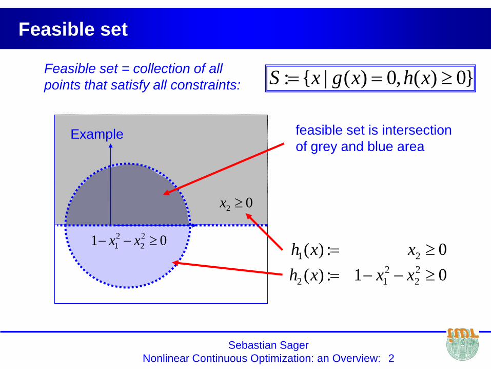
feasible set is intersection
of grey and blue area
Feasible set
Feasible set = collection of all
points that satisfy all constraints:
Example
}0)(,0)(|{: xhxgxS
02 x
01 2
2
2
1 xx
01:)(
0:)(2
2
2
12
21
xxxh
xxh

Sebastian Sager
Nonlinear Continuous Optimization: an Overview: 3
Local and global optima
f(x)
x
Global Minimum
Local Minimum
Local Minimum
Sebastian Sager
Nonlinear Continuous Optimization: an Overview: 4
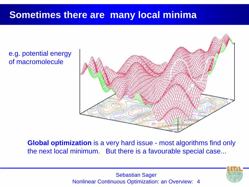
Sometimes there are many local minima
e.g. potential energy
of macromolecule
Global optimization is a very hard issue - most algorithms find only
the next local minimum. But there is a favourable special case...

Sebastian Sager
Nonlinear Continuous Optimization: an Overview: 5
Convex functions
Convex: all connecting
lines are above graph
Non-convex: some connecting
lines are not above graph
Sebastian Sager
Nonlinear Continuous Optimization: an Overview: 6
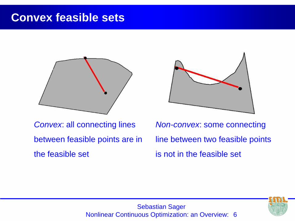
Convex feasible sets
Convex: all connecting lines
between feasible points are in
the feasible set
Non-convex: some connecting
line between two feasible points
is not in the feasible set

Sebastian Sager
Nonlinear Continuous Optimization: an Overview: 7
Convex problems
Convex problem if
f(x) is convex and the feasible set is convex
One can show: For convex problems, every local minimum is also a global minimum.
It is sufficient to find local minima!
Sebastian Sager
Nonlinear Continuous Optimization: an Overview: 8
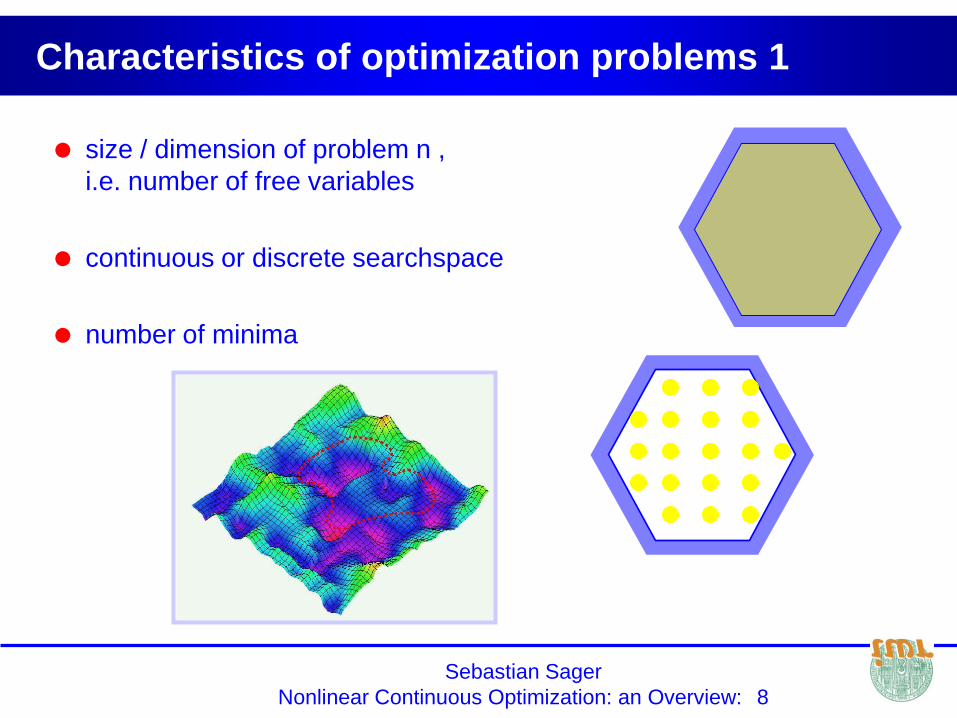
Characteristics of optimization problems 1
size / dimension of problem n ,
i.e. number of free variables
continuous or discrete searchspace
number of minima
Sebastian Sager
Nonlinear Continuous Optimization: an Overview: 9
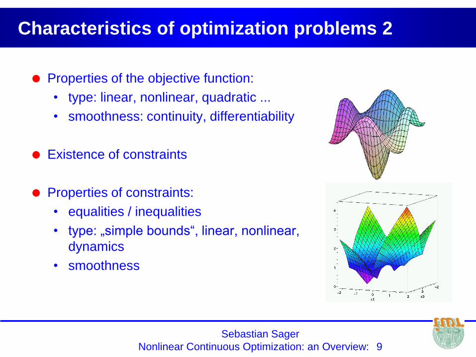
Characteristics of optimization problems 2
Properties of the objective function:
• type: linear, nonlinear, quadratic ...
• smoothness: continuity, differentiability
Existence of constraints
Properties of constraints:
• equalities / inequalities
• type: „simple bounds“, linear, nonlinear,
dynamics
• smoothness
Sebastian Sager
Nonlinear Continuous Optimization: an Overview: 10
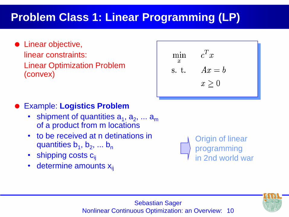
Problem Class 1: Linear Programming (LP)
Linear objective,
linear constraints:
Linear Optimization Problem(convex)
Example: Logistics Problem
• shipment of quantities a1, a2, ... am
of a product from m locations
• to be received at n detinations in quantities b1, b2, ... bn
• shipping costs cij
• determine amounts xij
Origin of linear
programming
in 2nd world war

Sebastian Sager
Nonlinear Continuous Optimization: an Overview: 11
Problem Class 2: Quadratic Programming (QP)
Quadratic objective and linear
constraints:
Quadratic Optimization Problem
(convex, if Q pos. def.)
Example: Markovitz mean variance portfolio optimization
• quadratic objective: portfolio variance (sum of the variances and
covariances of individual securities)
• linear constraints specify a lower bound for portfolio return
QPs play an important role as subproblems in nonlinear optimization
Sebastian Sager
Nonlinear Continuous Optimization: an Overview: 12
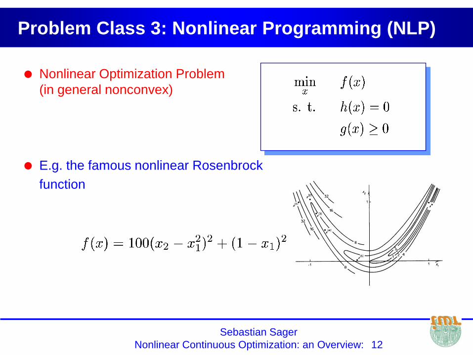
Problem Class 3: Nonlinear Programming (NLP)
Nonlinear Optimization Problem
(in general nonconvex)
E.g. the famous nonlinear Rosenbrock
function
Sebastian Sager
Nonlinear Continuous Optimization: an Overview: 13
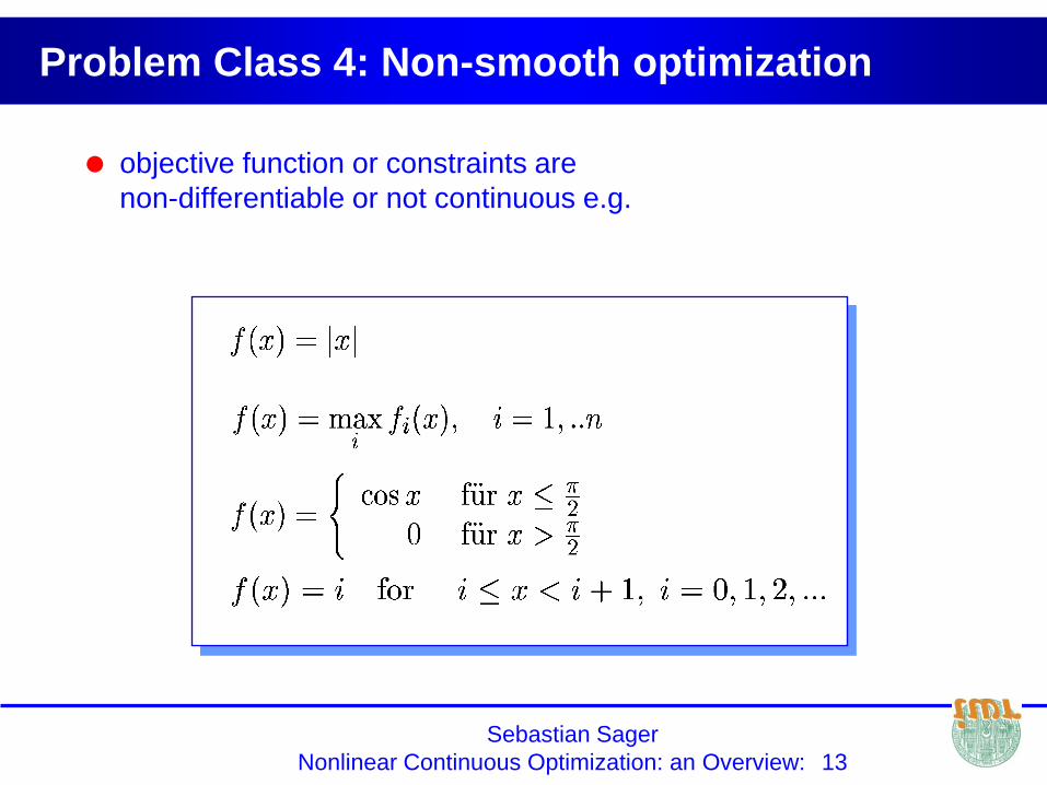
Problem Class 4: Non-smooth optimization
objective function or constraints are
non-differentiable or not continuous e.g.
Sebastian Sager
Nonlinear Continuous Optimization: an Overview: 14
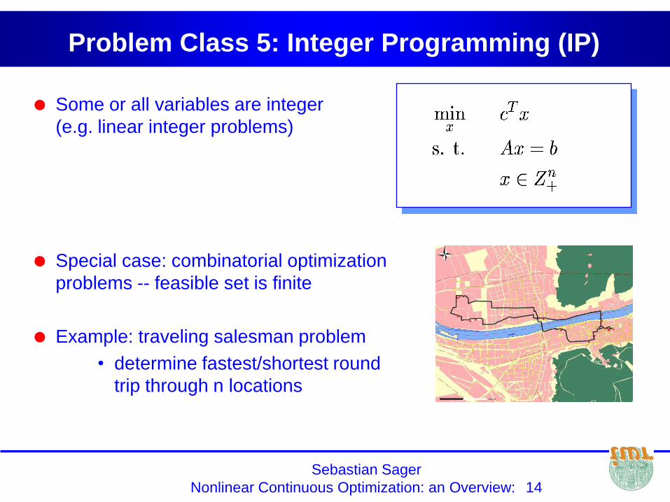
Some or all variables are integer
(e.g. linear integer problems)
Special case: combinatorial optimization
problems -- feasible set is finite
Example: traveling salesman problem
• determine fastest/shortest round
trip through n locations
Problem Class 5: Integer Programming (IP)
Sebastian Sager
Nonlinear Continuous Optimization: an Overview: 15
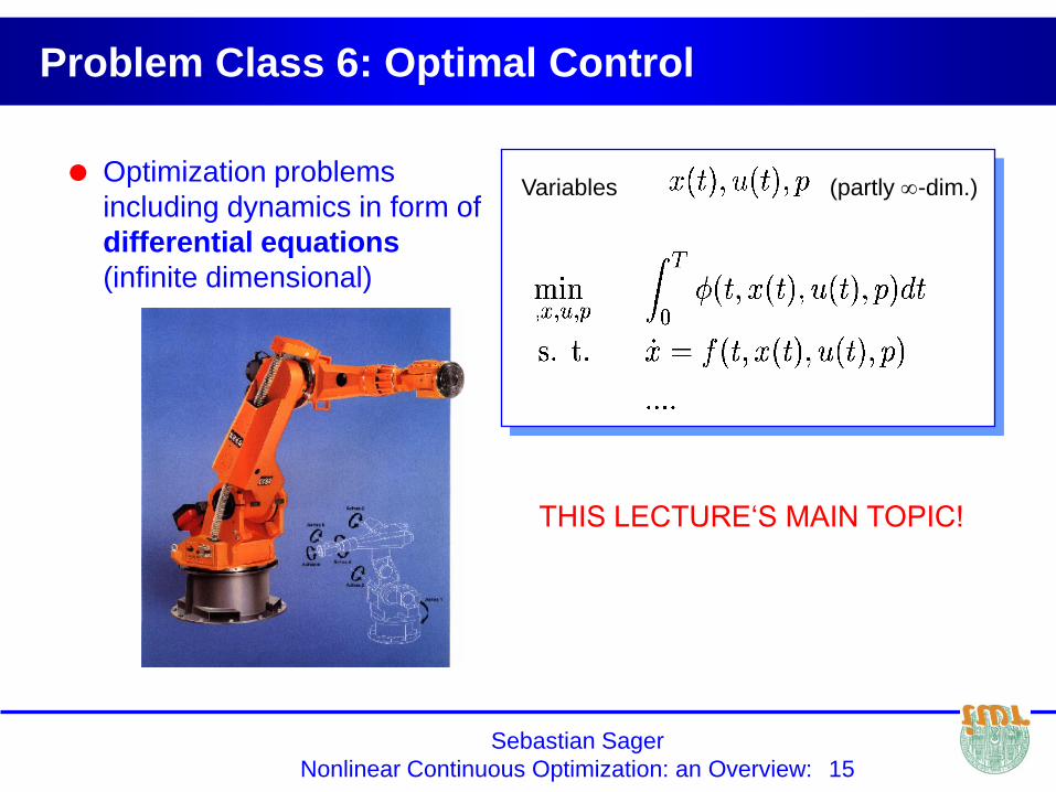
Problem Class 6: Optimal Control
Optimization problems
including dynamics in form of
differential equations
(infinite dimensional)
Variables (partly -dim.)
THIS LECTURE‘S MAIN TOPIC!

Sebastian Sager
Nonlinear Continuous Optimization: an Overview: 16
Nonlinear Programming (Problem Class 3)
f objective function / cost function
g equality constraints
h inequality constraints
f,g,h shall be smooth (twice differentiable) functions
kn
ln
n
RRDh
RRDg
RRDf
xh
xg
xf
ts
:
:
:
0)(
0)(
)(min
..
General problem formulation:
Sebastian Sager
Nonlinear Continuous Optimization: an Overview: 17
Overview of presentation
Optimization: basic definitions and concepts
Introduction to important classes of optimization problems
Introduction to linear programming
Introduction to nonlinear optimization algorithms
• Theory
• Algorithms for unconstrained problems
Some other popular optimization methods

Sebastian Sager
Nonlinear Continuous Optimization: an Overview: 18
Derivatives
First and second derivatives of the objective function or the
constraints play an important role in optimization
The first order derivatives are called the gradient (of the resp. fct)
and the second order derivatives are called the Hessian matrix

Sebastian Sager
Nonlinear Continuous Optimization: an Overview: 19
sufficient condition:
x* stationary and 2f(x*) positive definite
necessary condition:
f(x*)=0 (stationarity)
Optimality conditions (unconstrained)
Assume that f is twice differentiable.
We want to test a point x* for local
optimality.
x*
nRxxf )(min
Sebastian Sager
Nonlinear Continuous Optimization: an Overview: 20
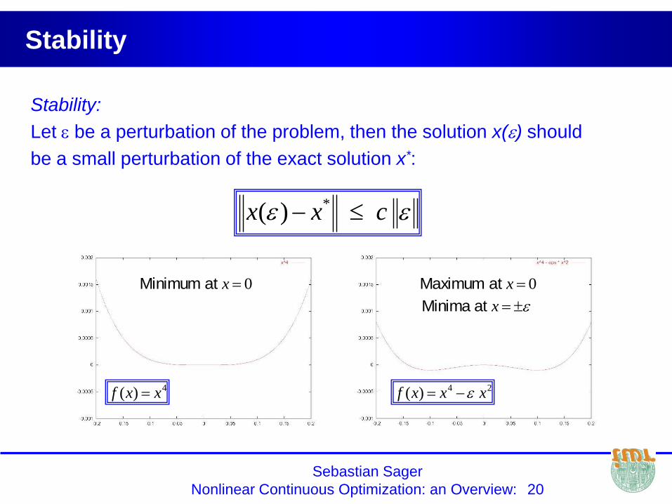
Stability
Stability:
Let e be a perturbation of the problem, then the solution x(e) should
be a small perturbation of the exact solution x*:
ee cxx *)(
4)( xxf 24)( xxxf e
0x at Minimum 0x at Maximum
ex at Minima
Sebastian Sager
Nonlinear Continuous Optimization: an Overview: 21
Stability
In the example problem the sufficient optimality conditions were not
satisfied ( 2f(x*) is not positive definite)
One can show:
Optima that satisfy the sufficient
optimality conditions are stable against
perturbations.

Sebastian Sager
Nonlinear Continuous Optimization: an Overview: 22
Types of stationary points
2f(x*) positive definite:
local minimum
2f(x*) negative definite:
local maximum
2f(x*) indefinite: saddle point
(a)-(c) x* is stationary: f(x*)=0

Sebastian Sager
Nonlinear Continuous Optimization: an Overview: 23
contour lines of f(x)
gradient vector
unconstrained minimum:
Ball on a spring without constraints
2
2
2
2
12min mxxx
Rx
)2,2()( 21 mxxxf
)2
,0(),()(0 *
2
*
1
* mxxxf
Sebastian Sager
Nonlinear Continuous Optimization: an Overview: 24
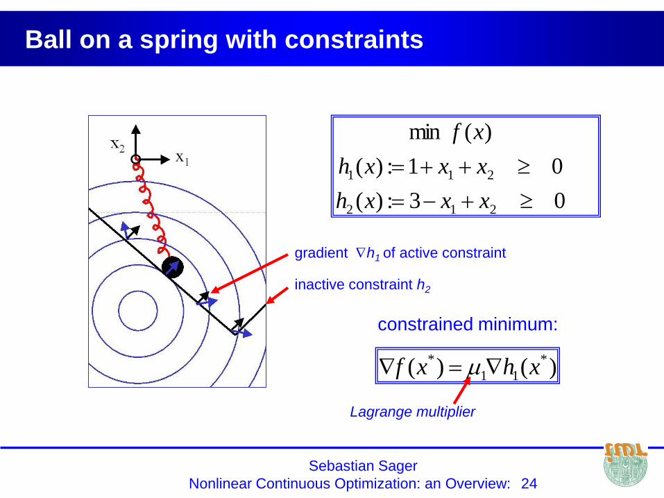
Ball on a spring with constraints
constrained minimum:
Lagrange multiplier
inactive constraint h2
03:)(
01:)(
)(min
212
211
xxxh
xxxh
xf
)()( *
11
* xhxf
gradient h1 of active constraint
Sebastian Sager
Nonlinear Continuous Optimization: an Overview: 25
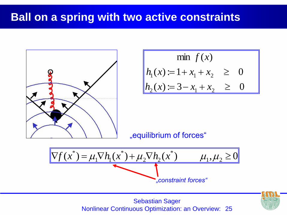
Ball on a spring with two active constraints
„equilibrium of forces“
„constraint forces“
0,)()()( 21
*
22
*
11
* xhxhxf
03:)(
01:)(
)(min
212
211
xxxh
xxxh
xf

Sebastian Sager
Nonlinear Continuous Optimization: an Overview: 26
Multipliers as „shadow prices“
What happens if we relax a constraint?
Feasible set becomes bigger,
so new minimum f(xe*) becomes smaller.
How much would we gain?
old constraint: h(x) 0
new constraint: h(x) + e 0
Multipliers show the hidden cost
of constraints.
ee )()( ** xfxf
Sebastian Sager
Nonlinear Continuous Optimization: an Overview: 27
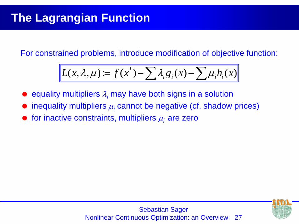
The Lagrangian Function
equality multipliers i may have both signs in a solution
inequality multipliers i cannot be negative (cf. shadow prices)
for inactive constraints, multipliers i are zero
For constrained problems, introduce modification of objective function:
)()()(:),,( * xhxgxfxL iiii
Sebastian Sager
Nonlinear Continuous Optimization: an Overview: 28
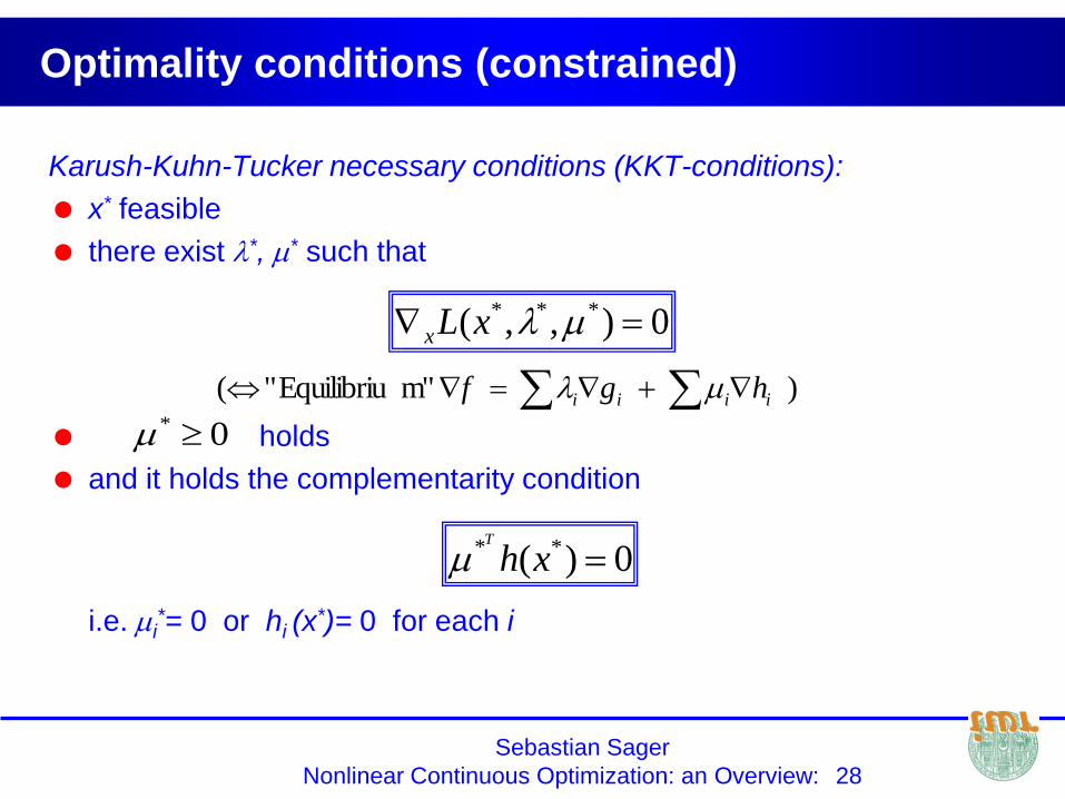
Karush-Kuhn-Tucker necessary conditions (KKT-conditions):
x* feasible
there exist *, * such that
holds
and it holds the complementarity condition
i.e. i*= 0 or hi (x
*)= 0 for each i
Optimality conditions (constrained)
0),,( *** xLx
0)( ** xhT
) m"Equilibriu" ( iiii hgf
0*

Sebastian Sager
Nonlinear Continuous Optimization: an Overview: 29
Overview of presentation
Optimization: basic definitions and concepts
Introduction to important classes of optimization problems
Introduction to linear programming
Introduction to nonlinear optimization algorithms
• Theory
• Algorithms for unconstrained problems
Some other popular optimization methods
Sebastian Sager
Nonlinear Continuous Optimization: an Overview: 30
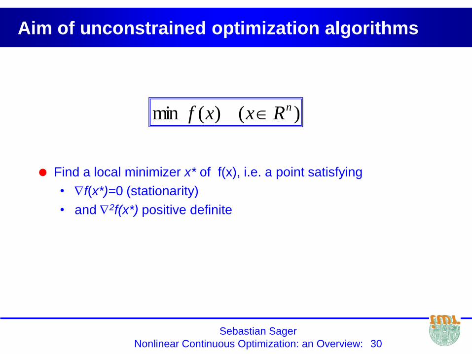
Aim of unconstrained optimization algorithms
Find a local minimizer x* of f(x), i.e. a point satisfying
• f(x*)=0 (stationarity)
• and 2f(x*) positive definite
)()(min nRxxf

Sebastian Sager
Nonlinear Continuous Optimization: an Overview: 31
Properties of Optimization Algorithms
Optimization algorithms are iterative, i.e. in general
they create an infinite (in practice finite) sequence of points
{xk } converging to the optimum x*
Order of convergence:
a sequence is said to converge with order r when r is the highest
number such that
r = 1 : linear convergence (c<1)
r = 2 : quadratic convergence (much better!)
0 = c <
Sebastian Sager
Nonlinear Continuous Optimization: an Overview: 32
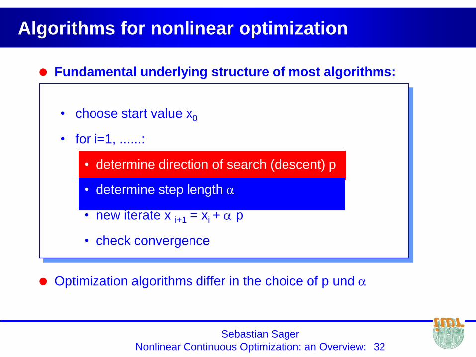
Fundamental underlying structure of most algorithms:
• choose start value x0
• for i=1, ......:
• determine direction of search (descent) p
• determine step length
• new iterate x i+1 = xi + p
• check convergence
Optimization algorithms differ in the choice of p und
Algorithms for nonlinear optimization

Sebastian Sager
Nonlinear Continuous Optimization: an Overview: 33
Basic algorithm
Search direction:
f should be decreased
in this direction
Step length:
solve1-d minimization
problem (exact or inexact):
)(minarg kkk pxf

Sebastian Sager
Nonlinear Continuous Optimization: an Overview: 34
Computation of step length
Ideal: Move to (global) minimum on the selected line
(univariate optimization, exact line search)
In practice: happy with approximate solution, perform only inexact line
search
Problem: how to guarantee sufficient decrease?
• Check e.g. if αk satisfies Armijo-Wolfe conditions
)(minarg kkk pxf
)(minarg kkk pxf
Sebastian Sager
Nonlinear Continuous Optimization: an Overview: 35
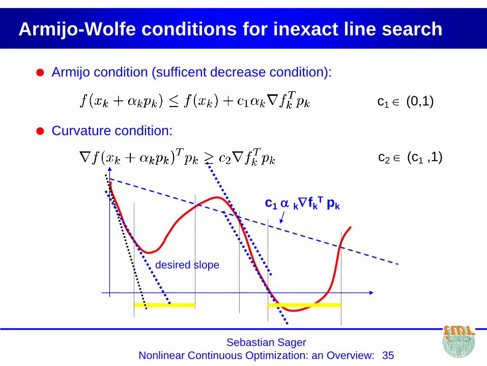
Armijo-Wolfe conditions for inexact line search
Armijo condition (sufficent decrease condition):
Curvature condition:
c1 kfkT pk
c1 (0,1)
c2 (c1 ,1)
desired slope
Sebastian Sager
Nonlinear Continuous Optimization: an Overview: 36
Computation of the search direction
For the determination of p frequently first and second order
derivatives of f are used
We discuss 4 algorithms:
• Steepest descent method
• Newton‘s method
• Quasi-Newton methods
• Sequential Quadratic Programming
Left out: conjugate gradients
Sebastian Sager
Nonlinear Continuous Optimization: an Overview: 37
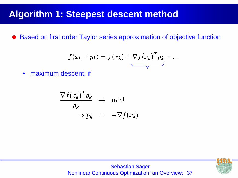
Algorithm 1: Steepest descent method
Based on first order Taylor series approximation of objective function
• maximum descent, if

Sebastian Sager
Nonlinear Continuous Optimization: an Overview: 38
Choose steepest descent search direction, perform (exact) line search:
search direction is perpendicular to level sets of f(x)
Steepest descent method
)( kk xfp )(1 kkkk xfxx
Gradient direction
Sebastian Sager
Nonlinear Continuous Optimization: an Overview: 39
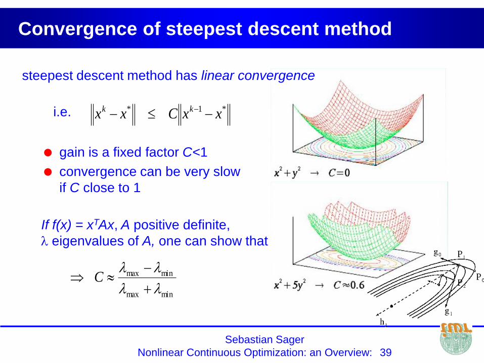
Convergence of steepest descent method
steepest descent method has linear convergence
*1* xxCxx kk
gain is a fixed factor C<1
convergence can be very slow
if C close to 1
If f(x) = xTAx, A positive definite,
eigenvalues of A, one can show that
minmax
minmax
C
i.e.
Sebastian Sager
Nonlinear Continuous Optimization: an Overview: 40
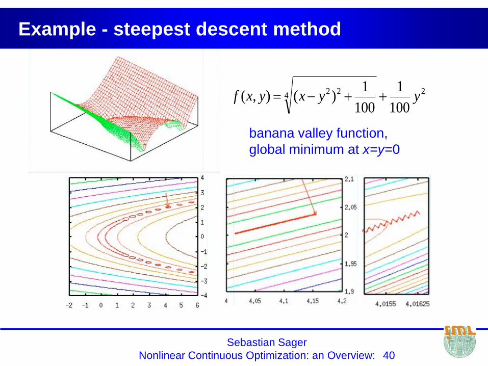
Example - steepest descent method
24
22
100
1
100
1)(),( yyxyxf
banana valley function,
global minimum at x=y=0
Sebastian Sager
Nonlinear Continuous Optimization: an Overview: 41
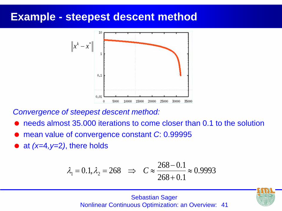
Example - steepest descent method
Convergence of steepest descent method:
needs almost 35.000 iterations to come closer than 0.1 to the solution
mean value of convergence constant C: 0.99995
at (x=4,y=2), there holds
9993.01.0268
1.0268268,1.0 21
C
*xxk

Sebastian Sager
Nonlinear Continuous Optimization: an Overview: 42
Algorithm 2: Newton‘s Method
Based on second order Taylor series approximation of f(x)
„Newton-Direction“
Sebastian Sager
Nonlinear Continuous Optimization: an Overview: 43
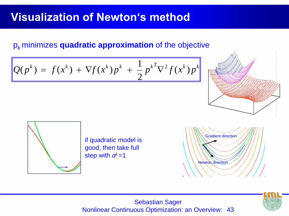
pk minimizes quadratic approximation of the objective
Visualization of Newton‘s method
kkTkkkkk pxfppxfxfpQ )(2
1 )( )( )( 2
Gradient direction
Newton direction
if quadratic model is
good, then take full
step with αk =1
Sebastian Sager
Nonlinear Continuous Optimization: an Overview: 44
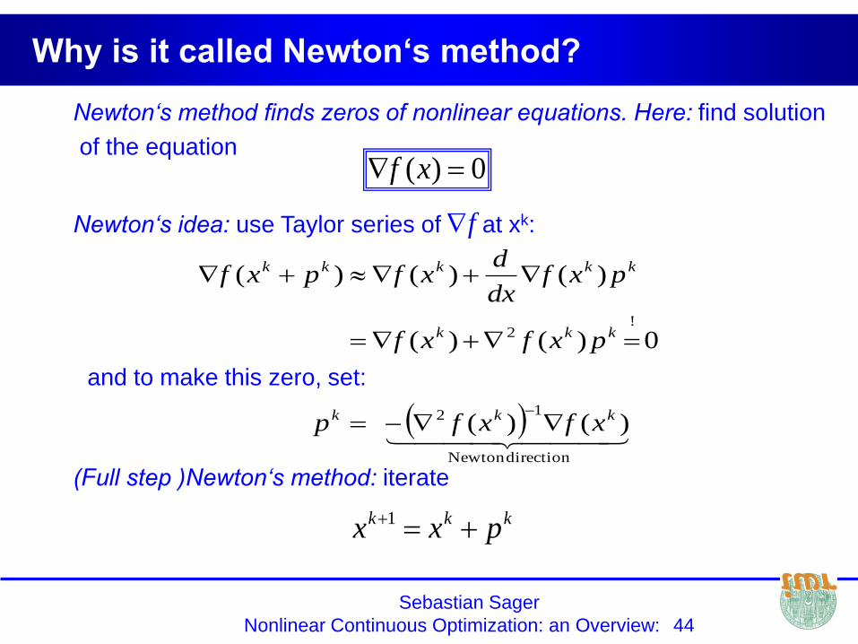
Newton‘s method finds zeros of nonlinear equations. Here: find solution
of the equation
Why is it called Newton‘s method?
0)( xf
directionNewton
12
!2
)()(
0)()(
)()()(
kkk
kkk
kkkkk
xfxfp
pxfxf
pxfdx
dxfpxf
Newton‘s idea: use Taylor series of f at xk:
kkk pxx 1
(Full step )Newton‘s method: iterate
and to make this zero, set:

Sebastian Sager
Nonlinear Continuous Optimization: an Overview: 45
Convergence of Newton‘s method
Newton‘s method has quadratic convergence
This is very fast close to a solution:
Doubles the correct digits in each iteration!
i.e.2
*1* xxCxx kk
Problem:
If the start value x0 of the iteration is near to a saddle point or
a maximum, the full step method converges to this saddle point
or maximum. Line search helps, but is only possible if p is
descent direction, i.e. if 2f positive definite.
Ensure this by: Levenberg-Marquard, or trust-region methods

Sebastian Sager
Nonlinear Continuous Optimization: an Overview: 46
Example - Newton‘s method
banana valley function,
global minimum at x=y=0
24
22
100
1
100
1)(),( yyxyxf
Sebastian Sager
Nonlinear Continuous Optimization: an Overview: 47
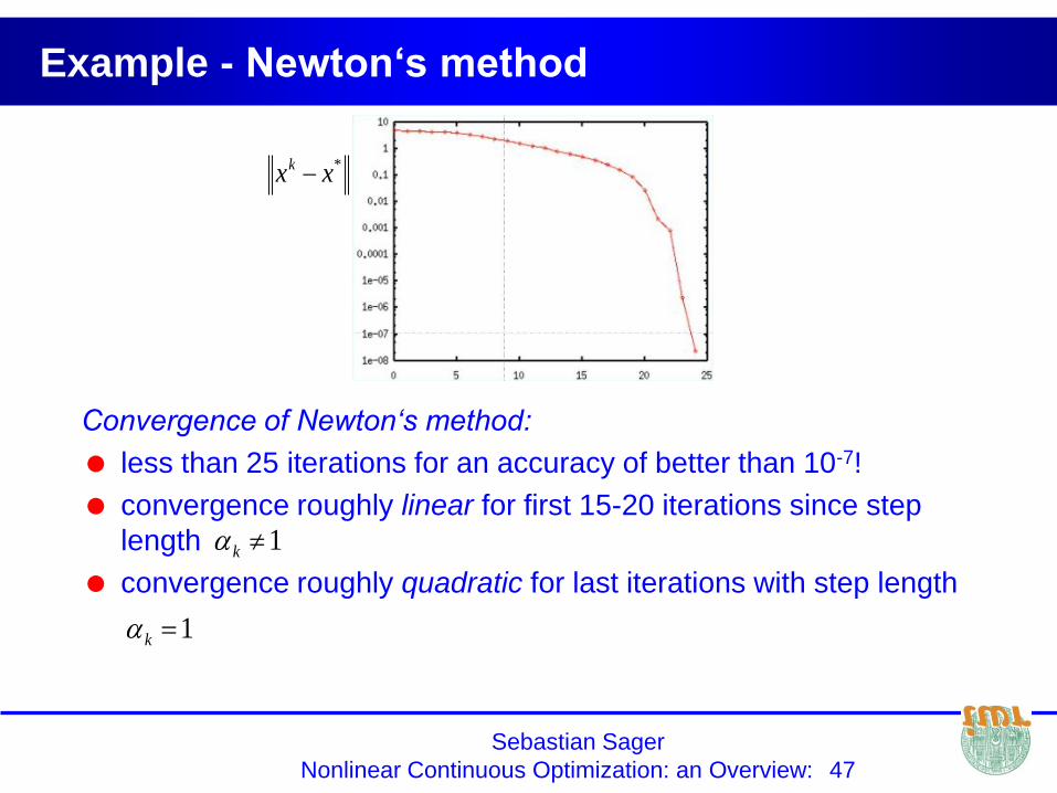
Example - Newton‘s method
Convergence of Newton‘s method:
less than 25 iterations for an accuracy of better than 10-7!
convergence roughly linear for first 15-20 iterations since step
length
convergence roughly quadratic for last iterations with step length
1k
1k
*xxk
Sebastian Sager
Nonlinear Continuous Optimization: an Overview: 48
Comparison of steepest descent and Newton
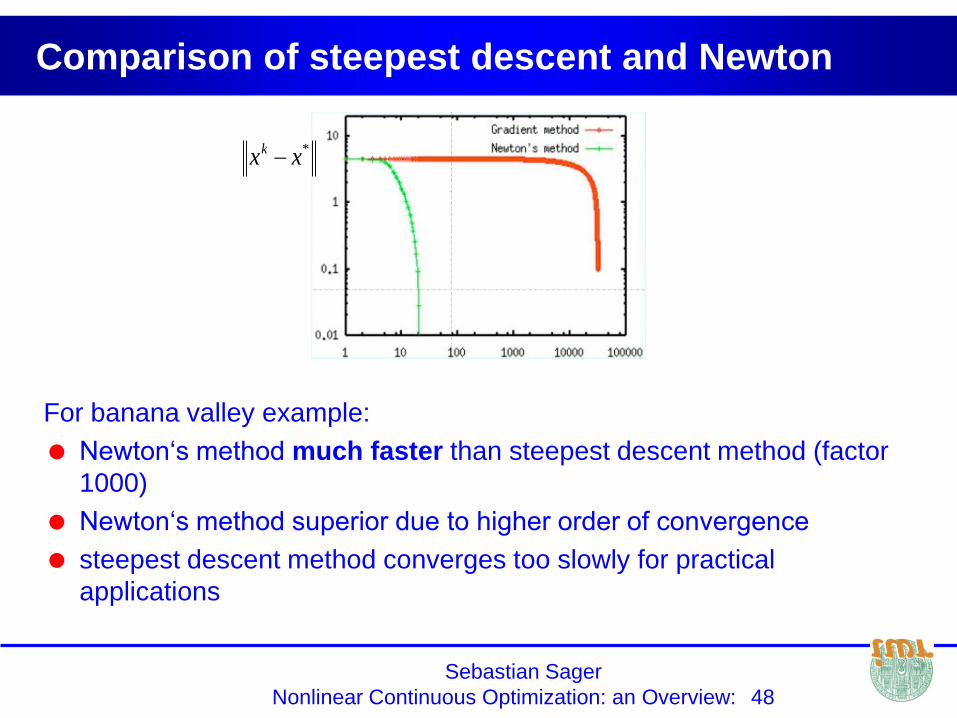
For banana valley example:
Newton‘s method much faster than steepest descent method (factor
1000)
Newton‘s method superior due to higher order of convergence
steepest descent method converges too slowly for practical
applications
*xxk

Sebastian Sager
Nonlinear Continuous Optimization: an Overview: 49
Algorithm 3: Quasi-Newton methods
In practice, evaluation of second derivatives
for the hessian is expensive!
)(
)(
2
11
kk
kk
kk
xfB
xfBxx
methods are collectively known as Quasi-Newton methods
)with)( : methoddescent steepest :case special( 1 IBxfBp kk
approximate hessian matrix 2f(xk)
also ensure that the approximation Bk is positive definite

Sebastian Sager
Nonlinear Continuous Optimization: an Overview: 50
Different Quasi-Newton methods:
simplified Newton method: keep hessian B constant
or: use same matrix B for several iterations:
if then update
or, even cheaper: use update-formulas for hessian...
Quasi-Newton methods
)( 02 xfB
max
1
k
k
x
x)( 12 kxfB

Sebastian Sager
Nonlinear Continuous Optimization: an Overview: 51
Quasi-Newton Update formulas
Idea: Given an hessian approximation Bk
find a new approximation Bk+1 that is similar to Bk but satisfies
f(xk) + Bk+1 (xk+1 - xk) = f(xk+1)
ADVANTAGES:
needs only evaluation of gradient f(xk) (same cost as steepest
descent), but incorporates second order information
additional advantage: can update the inverse Bk-1 directly
EXAMPLES:
Symmetric Broyden-update
DFP-update (Davidon, Fletcher, Powell)
BFGS-update (Broyden, Fletcher, Goldfarb, Shanno) (most widely used)
Sebastian Sager
Nonlinear Continuous Optimization: an Overview: 52
Convergence
Quasi-Newton update methods converge locally superlinearly,i.e.,
this is typically much faster than linear!
updates converge globally,
if Bk remain positive definite and line search is used
Quasi-Newton methods most popular method for medium scale
problems (up to 10000 variables)
0 with **1
k
k
k
k cxxcxx

Sebastian Sager
Nonlinear Continuous Optimization: an Overview: 53
Algorithm 4: SQP-method
Constrained problem:
0)(
0)(
2
1)(min
xxh)h(x
xxg)g(x
xHxxf
Tkk
Tkk
kTTk
x
0)(
0)(
)(min
xh
xg
xf
Idea: Consider successively quadratic approximations of the problem:
Sebastian Sager
Nonlinear Continuous Optimization: an Overview: 54
SQP-method
if we use the exact Hessian of the Lagrangian
this leads to a Newton-method for the optimality conditions and
feasibility.
with update-formulas for Hk, we obtain quasi-Newton SQP-methods.
if we use appropriate update-formulas, we can have superlinear
convergence.
global convergence can be achieved by using a stepsize strategy.
),,(2 xLH

Sebastian Sager
Nonlinear Continuous Optimization: an Overview: 55
SQP algorithm
0. Start with k=0, start value x0 and H0=I
1. Compute f(xk), g(xk), h(xk), f(xk), g(xk), h(xk)
2. If xk feasible and
then stop convergence achieved
3. Solve quadratic problem and get xk
4. Perform line search and get stepsize tk
5. Iterate
6. Update hessian
7. k=k+1, goto step 1
e ),,(xL
kkkk xtxx 1

Sebastian Sager
Nonlinear Continuous Optimization: an Overview: 56
Solution of the quadratic program
Unconstrained case:
H must be positive definite, otherwise the optimization problem has
no solution
necessary optimality condition:
=> use cholesky-method or cg-method to solve
dgHdd tt 2
1min
0 gHd
Sebastian Sager
Nonlinear Continuous Optimization: an Overview: 57
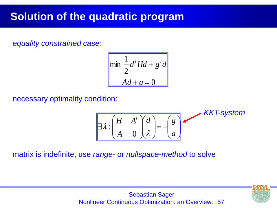
Solution of the quadratic program
equality constrained case:
necessary optimality condition:
matrix is indefinite, use range- or nullspace-method to solve
0
2
1min
aAd
dgHdd tt
a
gd
A
AH t
0:
KKT-system

Sebastian Sager
Nonlinear Continuous Optimization: an Overview: 58
Solution of the quadratic program
equality and inequality constrained case:
use active-set-strategy
aim: find out which inequalities are active and which not
0
0
2
1min
bBd
aAd
dgHdd tt
Sebastian Sager
Nonlinear Continuous Optimization: an Overview: 59
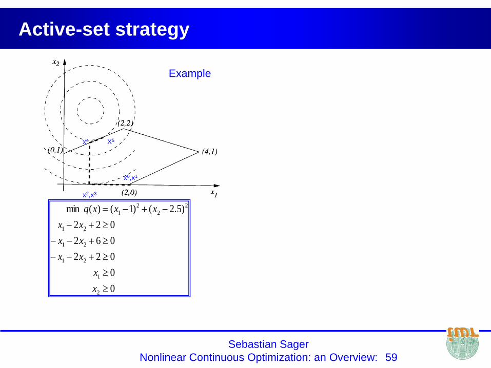
Active-set strategy
x0,x1
x2,x3
x4 X5
0
0
022
062
022
)5.2()1()(min
2
1
21
21
21
2
2
2
1
x
x
xx
xx
xx
xxxq
Example

Sebastian Sager
Nonlinear Continuous Optimization: an Overview: 60
Active-set strategy
x0,x1
x2,x3
x4 X5
0
0
022
062
022
)5.2()1()(min
2
1
21
21
21
2
2
2
1
x
x
xx
xx
xx
xxxq
• x0=(2,0), W0={3,5}
negative multiplier with respect to constraint 3,
remove constraint 3
Example
Sebastian Sager
Nonlinear Continuous Optimization: an Overview: 61
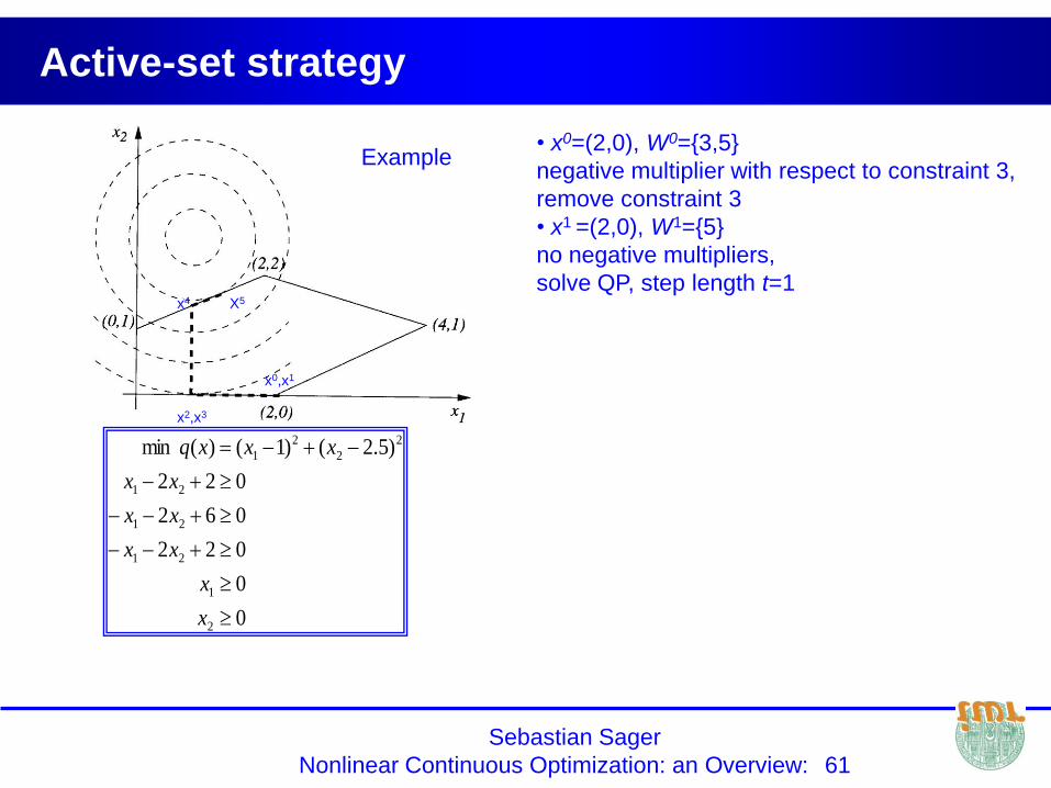
Active-set strategy
x0,x1
x2,x3
x4 X5
0
0
022
062
022
)5.2()1()(min
2
1
21
21
21
2
2
2
1
x
x
xx
xx
xx
xxxq
• x0=(2,0), W0={3,5}
negative multiplier with respect to constraint 3,
remove constraint 3
• x1 =(2,0), W1={5}
no negative multipliers,
solve QP, step length t=1
Example

Sebastian Sager
Nonlinear Continuous Optimization: an Overview: 62
Active-set strategy
x0,x1
x2,x3
x4 X5
0
0
022
062
022
)5.2()1()(min
2
1
21
21
21
2
2
2
1
x
x
xx
xx
xx
xxxq
• x0=(2,0), W0={3,5}
negative multiplier with respect to constraint 3,
remove constraint 3
• x1 =(2,0), W1={5}
no negative multipliers,
solve QP, step length t=1
• x2 =(1,0),W2={5}
negative multiplier respect to constraint 5
remove constraint 5
Example

Sebastian Sager
Nonlinear Continuous Optimization: an Overview: 63
Active-set strategy
x0,x1
x2,x3
x4 X5
0
0
022
062
022
)5.2()1()(min
2
1
21
21
21
2
2
2
1
x
x
xx
xx
xx
xxxq
• x0=(2,0), W0={3,5}
negative multiplier with respect to constraint 3,
remove constraint 3
• x1 =(2,0), W1={5}
no negative multipliers,
solve QP, step length t=1
• x2 =(1,0),W2={5}
negative multiplier respect to constraint 5
remove constraint 5
• x3=(1,0), W3={}
no negative multipliers
solve QP, step length t<1, constraint 1 gets
active
Example

Sebastian Sager
Nonlinear Continuous Optimization: an Overview: 64
Active-set strategy
x0,x1
x2,x3
x4 X5
0
0
022
062
022
)5.2()1()(min
2
1
21
21
21
2
2
2
1
x
x
xx
xx
xx
xxxq
• x0=(2,0), W0={3,5}
negative multiplier with respect to constraint 3,
remove constraint 3
• x1 =(2,0), W1={5}
no negative multipliers,
solve QP, step length t=1
• x2 =(1,0),W2={5}
negative multiplier respect to constraint 5
remove constraint 5
• x3=(1,0), W3={}
no negative multipliers
solve QP, step length t<1, constraint 1 gets
active
• x4=(1,1.5), W4={1},
no negative multipliers,
solve QP, step length t=1
Example

Sebastian Sager
Nonlinear Continuous Optimization: an Overview: 65
Active-set strategy
x0,x1
x2,x3
x4 X5
0
0
022
062
022
)5.2()1()(min
2
1
21
21
21
2
2
2
1
x
x
xx
xx
xx
xxxq
• x0=(2,0), W0={3,5}
negative multiplier respect to constraint 3,
remove constraint 3
• x1 =(2,0), W1={5}
no negative multipliers,
solve QP, step length t=1
• x2 =(1,0),W2={5}
negative multiplier respect to constraint 5
remove constraint 5
• x3=(1,0), W3={}
no negative multipliers
solve QP, step length t<1, constraint 1 gets
active
• x4=(1,1.5), W4={1},
no negative multipliers,
solve QP, step length t=1
• x5=(1.4,1.7), W5={3,5}
all multipliers positive,
solution
Example
Sebastian Sager
Nonlinear Continuous Optimization: an Overview: 66
Overview of presentation
Optimization: basic definitions and concepts
Introduction to important classes of optimization problems
Introduction to continuous optimization algorithms
Some other popular optimization methods
• Direct search methods
• Simulated annealing, great deluge, threshold
acceptance
• Genetic algorithms, Particle swarm methods
Sebastian Sager
Nonlinear Continuous Optimization: an Overview: 67
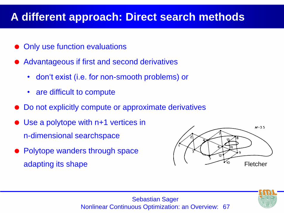
A different approach: Direct search methods
Only use function evaluations
Advantageous if first and second derivatives
• don‘t exist (i.e. for non-smooth problems) or
• are difficult to compute
Do not explicitly compute or approximate derivatives
Use a polytope with n+1 vertices in
n-dimensional searchspace
Polytope wanders through space
adapting its shape Fletcher

Sebastian Sager
Nonlinear Continuous Optimization: an Overview: 68
Direct search methods
Nelder-Mead:
• worst point is replaced by a combination of reflection, expansion, contraction, scaling... Operations
Other variants:
• all except best point are replaced
• ...
Belong to the most frequently used optimization algorithms in practice
But are much slower than BFGS or CG

Sebastian Sager
Nonlinear Continuous Optimization: an Overview: 69
Treatment of constraints
Approximation of constrained optimization by unconstrained
Penalty methods: penalty term for violation of constraints
Barrier methods: penalty term for getting close to boundary
Adjust penalty / barrier parameter (series of subproblems):
c approximation becomes increasingly accurate
Resulting objective function is typically ill-conditioned
Use of some unconstrained methods possible with special care
Penalty and barrier methods

Sebastian Sager
Nonlinear Continuous Optimization: an Overview: 70
Treatment of constraints
Directly solve first order optimality conditions for constrained problem
Involves Lagrange-Function (combining objective function and
constraints)
Lagrange methods
Sebastian Sager
Nonlinear Continuous Optimization: an Overview: 71
Some algorithms for global optimization
Exact algorithms for combinatorial problems, e.g.
• Enumeration
• Branch and Bound
Stochastic algorithms, e.g.
• Monte-Carlo
• Tabu-Search
• Simulated Anneling / Threshold Acceptance / Great Deluge
Algorithm
Incomplete methods, e.g.
• Particle swarm method
Evolutionary Computation
• Genetic Algorithms + Evolutionary strategies

Sebastian Sager
Nonlinear Continuous Optimization: an Overview: 72
Simulated Annealing, Threshold Acceptance
& Great Deluge Algorithms
For illustrational purposes in this case:
• consider maximization problem
Basic Idea:
• do not demand improvement (i.e. ascent) in every step
• also allow temporary decrease of objective function in order to
leave local optima and find global optimum
Sebastian Sager
Nonlinear Continuous Optimization: an Overview: 73
Simulated Annealing, Threshold Acceptance
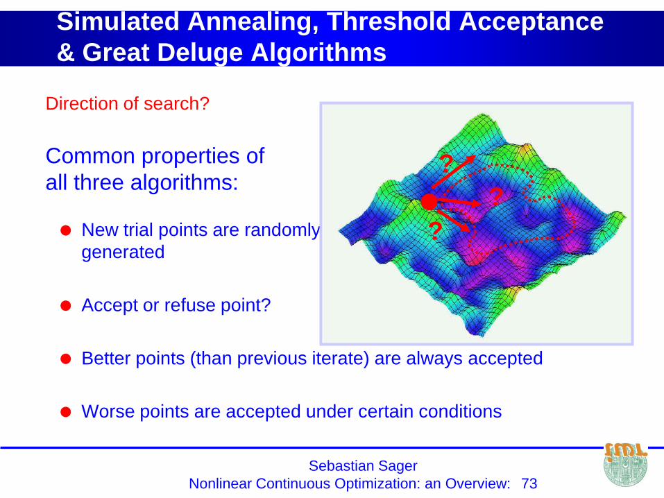
& Great Deluge Algorithms
New trial points are randomly
generated
Accept or refuse point?
Better points (than previous iterate) are always accepted
Worse points are accepted under certain conditions
?
?
?
Common properties of
all three algorithms:
Direction of search?
Sebastian Sager
Nonlinear Continuous Optimization: an Overview: 74
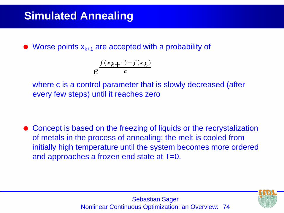
Simulated Annealing
Worse points xk+1 are accepted with a probability of
where c is a control parameter that is slowly decreased (after
every few steps) until it reaches zero
Concept is based on the freezing of liquids or the recrystalization
of metals in the process of annealing: the melt is cooled from
initially high temperature until the system becomes more ordered
and approaches a frozen end state at T=0.

Sebastian Sager
Nonlinear Continuous Optimization: an Overview: 75
Threshold Acceptance
Worse points xk+1 are only accepted if the difference is
not larger than a threshold T
Threshold value is successively decreased to zero
T
Sebastian Sager
Nonlinear Continuous Optimization: an Overview: 76
Great Deluge
Worse points xk+1 are only accepted if
they are larger than the current lower
bound S
S is continuously increased
S can be interpreted as the water level
during the biblical Flood ....
Sebastian Sager
Nonlinear Continuous Optimization: an Overview: 77
Genetic algorithms 1
Abstractions of biological evolution
General idea: Design optimization process that works according to
evolution and natural adaption processes
Genetic algorithms (GAs) require encoding of the optimization variables
as finite length strings over some finite alphabet
(typically bit strings)
GAs do not work with single iterates, but use populations of
chromosomes
GAs only use function evaluations , no derivatives,
objective function is called fitness function
Sebastian Sager
Nonlinear Continuous Optimization: an Overview: 78
Genetic algorithms 2
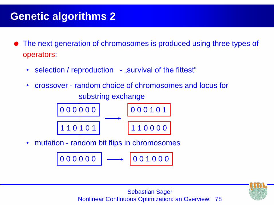
The next generation of chromosomes is produced using three types of
operators:
• selection / reproduction - „survival of the fittest“
• crossover - random choice of chromosomes and locus for
substring exchange
• mutation - random bit flips in chromosomes
0 0 0 0 0 0 0 0 1 0 0 0
0 0 0 0 0 0
1 1 0 1 0 1
0 0 0 1 0 1
1 1 0 0 0 0
Sebastian Sager
Nonlinear Continuous Optimization: an Overview: 79
Particle swarm optimization
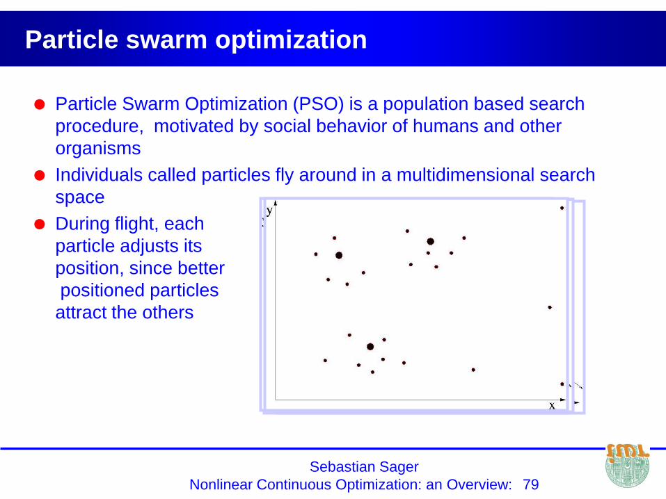
Particle Swarm Optimization (PSO) is a population based search
procedure, motivated by social behavior of humans and other
organisms
Individuals called particles fly around in a multidimensional search
space
During flight, each
particle adjusts its
position, since better
positioned particles
attract the others
Sebastian Sager
Nonlinear Continuous Optimization: an Overview: 80
Summary: Optimization Overview
Optimization problems can be (un)constrained, (non)convex, (non)linear,
(non)smooth, continuous/integer,(in)finite dimensional, ...
Here: try to find local minima of smooth nonlinear problems: f(x*)=0
(resp. L(x*, *, * )=0)
Starting at an initial guess x0 , most methods iterate x i+1 = xi + i pi with
search direction pi and step length i
Search direction can be chosen differently
• steepest descent (intuitive, but slow and rarely used in practice)
• Newton‘s method (very fast if Hessian cheaply available)
• Quasi-Newton methods (cheap,fast, and popular, e.g. BFGS)
• SQP methods relate to Newton‘s method
• CG method (good for very large scale problems)
Other popular methods (usually not recommended): direct search,
simulated annealing, genetic algorithms, ...

Sebastian Sager
Nonlinear Continuous Optimization: an Overview: 81
Literature
J. Nocedal, S. Wright: Numerical Optimization, Springer, 1999
P. E. Gill, W. Murray, M. H. Wright: Practical Optimization, Academic
Press, 1981
R. Fletcher, Practical Methods of Optimization, Wiley, 1987
D. E. Luenberger: Linear and Nonlinear Programming, Addison
Wesley, 1984
D. E. Goldberg: Genetic Algorithms in Search, Optimization and
Machine Learning, Addison Wesley, 1989
K. Neumann, M. Morlock: Operations Research, Carl Hanser Verlag,
1993