CHAPTER XII: NONLINEAR OPTIMIZATION CONDITIONS

copyright 1997 Bruce A. McCarl and Thomas H. Spreen

CHAPTER XII: NONLINEAR OPTIMIZATION CONDITIONS ......................................... 12-1

12.1 Optimality Conditions ............................................................................................ 12-1

12.1.1 Unconstrained Optimization ................................................................... 12-1

12.1.1.1 Univariate ................................................................................. 12-2

12.1.1.2 Multivariate functions .............................................................. 12-2

12.1.2 Global Optima-Concavity and Convexity .............................................. 12-3

12.1.3 Constrained Optimization ....................................................................... 12-4

12.1.3.1 Equality Constraints - The Lagrangian ................................... 12-5

12.1.3.1.1 Second Order Conditions - Constraint Qualifications:

Convexity and Concavity ............................................... 12-7

12.1.3.1.2 Interpretation of Lagrange Multipliers ...................... 12-8

12.1.3.2 Inequality Constraints - Kuhn Tucker Theory ....................... 12-10

12.1.3.2.1 Example 1 ............................................................... 12-11

12.1.3.2.2 Example 2 ............................................................... 12-12

12.1.4 Usage of Optimality Conditions ........................................................... 12-13

12.2 Notes on Solution of Nonlinear Programming Models ...................................... 12-13

12.3 Expressing Nonlinear Programs in Conjunction with GAMS ............................ 12-14

References .................................................................................................................... 12-16

copyright 1997 Bruce A. McCarl and Thomas H. Spreen

CHAPTER XII: NONLINEAR OPTIMIZATION CONDITIONS

The previous material deals largely with linear optimization problems. We now turn our attention to

continuous, certain, nonlinear optimization problems. The problems amenable to analysis using the

methods in this chapter relax the LP additivity and proportionality assumptions.

The nonlinear optimization problem is important in a number of settings. This chapter will lay the

ground work for several later chapters where price endogenous and risk problems are formulated as

nonlinear optimization problems. Optimality conditions for the problems will be treated followed by

brief discussion of solution principles.

12.1 Optimality Conditions This section is devoted to the characterization of optimality conditions for nonlinear programming

problems. These characterizations depend upon both first order conditions for identification of

stationary points and second order conditions for discovery of the nature of the stationary points

found. Consideration of types of optimum involves the topics of concavity and convexity. Thus,

concavity and convexity are discussed. The presentation will not be extremely rigorous. Those

interested in more rigorous treatments should consult books like Hadley, or Bazaraa and Shetty.

Nonlinear optimization problems may be constrained or unconstrained. Optimality conditions for

unconstrained problems are ordinarily developed in calculus classes and will be briefly reviewed.

Lagrangian multiplier and Kuhn Tucker based approaches are used to treat constrained problems and

will be discussed here.

12.1.1 Unconstrained Optimization

Unconstrained optimization is a topic in calculus classes. Such problems may contain one or N

variables.

12.1.1.1 Univariate

Problems with a single variable are called univariate. The univariate optimum for Y = f(X) occurs at

points where the first derivative of f(X) with respect to X (f '(X)) equals zero. However, points which

have zero first derivatives do not necessarily constitute a minimum or maximum. The second

derivative is used to discover character of a point. Points at which a relative minimum occurs have a

positive second derivative at that point while relative maximum occurs at points with a negative

second derivative. Zero second derivatives are inconclusive.

It is important to distinguish between local and global optima. A local optimum arises when one

finds a point whose value in the case of a maximum exceeds that of all surrounding points but may

not exceed that of distant points. The second derivative indicates the shape of functions and is useful

in indicating whether the optimum is local or global. The second derivative is the rate of change in

the first derivative. If the second derivative is always negative (positive) that implies that any

maximum (minimum) found is a global result. Consider a maximization problem with a negative

second derivative for which f '(X*)=0. This means the first derivative was > 0 for X < X

* and was < 0

for X > X*. The function can never rise when moving away from X

* because of the sign of the

second derivative. An everywhere positive second derivative indicates a global minimum will be

copyright 1997 Bruce A. McCarl and Thomas H. Spreen 12-2

found if f '( X*)=0, while a negative indicates a global maximum.

12.1.1.2 Multivariate functions The univariate optimization results have multivariate analogues. In the multivariate case, partial

derivatives are used, and a set of simultaneous conditions is established. The first and second

derivatives are again key to the optimization process, excepting now that a vector of first derivatives

and a matrix of second derivatives is involved.

There are several terms to review. First, the gradient vector, )f(X x , is the vector of first order

partial derivatives of a multivariate function with respect to each of the variables evaluated at the

point X .

where )(X f / X j stands for the partial derivative of f(X) with respect to Xj evaluated at X , and X

depicts 1X , 2X ,..., nX . The second derivatives constitute the Hessian matrix,

The Hessian matrix, evaluated at X , is an NxN symmetric matrix of second derivatives of the

function with respect to each variable pair.

The multivariate analogue of the first derivative test is that an X must be found so that all terms of

the gradient vector simultaneously equal zero. The multivariate version of the second derivative test

involves examination of the Hessian matrix at X . If that matrix is positive definite then the point

X is a local minimum, whereas if the Hessian matrix is negative definite then the point is a local

maximum. If the Hessian matrix is neither positive nor negative definite, then no conclusion can be

made about whether this point is a maximum or minimum and one must conclude it is an inflection or

saddle point.

12.1.2 Global Optima-Concavity and Convexity

The characterization of minimum and maximum points whether global or local is related to the

concavity and convexity of functions. A univariate concave function has a negative second

derivative everywhere and guarantees global maximum. A univariate convex function has a positive

derivative everywhere yielding a global minimum. The multivariate analogues exhibit the proper

definiteness of the Hessian matrix at all X points.

It is obviously desirable when dealing with optimization problems that global optimum be found.

Thus, maximization problems are frequently assumed to be concave while minimization problems are

assumed to be convex. Functions may also be locally concave or convex when the second derivative

or Hessian only satisfies the sign convention in a region. Optimization problems over such functions

can only yield local optimum.

Concavity of functions has been defined in another fashion. Concave functions exhibit the property

X

)(X f = )f(X

j

j

X X

)f(X=)H(X

ji

2ij


that, given any two points X1 and X2 in the domain of the function, a line joining those points always

lies below the function. Mathematically, this is expressed as

Note that f(X1) + (1-)f(X2) is a line between f(X1) and f(X2) and that concavity requires this line to

fall below the true function (f(X1 + (1-)X2)) everywhere below this function.

Similarly, a line associated with two points on a convex function must lie above the true function

1 0

) X f() -1 ( + ) X f( ) X) -1 ( + X f( 2121

Concavity and convexity occur locally or globally. A function is globally concave if the conditions

hold for all X or is locally concave or convex if the functions satisfy the conditions in some

neighborhood.

The optimality conditions may be restated in terms of concavity and convexity. Namely, a

multivariate function for which a stationary point X has been discovered has: a) a local maximum

at X if the function is locally concave, b) a global maximum if the function is concave throughout

the domain under consideration, c) a local minimum at X if the function is locally convex, d) a

global minimum at X if the function is strictly convex, and e) a saddle point if the function is

neither concave nor convex. At the stationary point, concavity and convexity for these conditions

may be evaluated either using the two formulas above or using the positive or negative definiteness

properties of the Hessian.

12.1.3 Constrained Optimization

The second major type of optimization problem is the constrained optimization problem. Two types

of constrained problems will be considered: those subject to equality constraints without sign

restricted variables and those subject to inequality constraints and/or sign restrictions on the

variables.

The optimality conditions for equality constrained optimization problems involve the Lagrangian and

associated optimality conditions. The solution of problems with inequality constraints and/or

variable sign restrictions relies on Kuhn-Tucker theory.

12.1.3.1 Equality Constraints - The Lagrangian Consider the problem

Maximize f(X)

s.t. gi(X) = bi for all I

where f (X) and gi (X) are functions of N variables and there are M equality constraints on the

problem. Optimization conditions for this problem were developed in the eighteenth century by

Lagrange. The Lagrangian approach involves first forming the function,

1 0

) X f( ) -1 ( + ) X f( )X)-1 ( + X f( 2121


)b(X)g( f(X)=)L(X, iii

i

where a new set of variables (i) are entered. These variables are called Lagrange multipliers. In

turn the problem is treated as if it were unconstrained with the gradient set to zero and the Hessian

examined. The gradient is formed by differentiating the Lagrangian function L(X,) with respect to

both X and . These resultant conditions are

.iallfor0)b)(Xg(

L

j allfor 0 = X

)(Xg

)Xf( =

X

L

ii

j

ii

ij

jX

In words, the first condition requires that at X the gradient vector of f (X) minus the sum of

times the gradient vector of each constraint must equal zero . The second condition says that at Xthe original constraints must be satisfied with strict equality. The first order condition yields a system

of N+M equations which must be simultaneously satisfied. In this case, the derivatives of the

objective function are not ordinarily driven to zero. Rather, the objective gradient vector is equated

to the Lagrange multipliers times the gradients of the constraints.

iallforbXas.t.

XcMax

i

j

jij

j

jj

These conditions are analogous to the optimality conditions of an LP consider a LP problem with N

variables and M binding constraints. The first order conditions using the Lagrangian would be

iallfor0)bXa(L

jallfor0acX

L

j

ijij

i

i

ijij

j

Clearly, this set of conditions is analogous to the optimality conditions on the LP problem when one

eliminates the possibility of zero variables and nonbinding constraints. Further, the Lagrange

multipliers are analogous to dual variables or shadow prices, as we will show below.

Use of the Lagrangian is probably again best illustrated by example. Given the problem

Minimize X2

1 + X22

s.t. X1 + X2 = 10

the Lagrangian function is

L(X,) = X2

1 + X22 - (X1 + X2 - 10)

Forming the Lagrange multiplier conditions leads to


0)10(

022

02

21

2

2

1

1

XXL

XX

L

XX

L

In turn, utilizing the first two conditions, we may solve for 1X and 2X in terms of and getting

1X = 2X = /2

Then plugging this into the third equation leads to the conclusion that

= 10; 1X = 2X = 5

This is then a stationary point for this problem and, in this case, is a relative minimum. We will

discuss the second order conditions below.

12.1.3 Second Order Conditions - Constraint Qualifications: Convexity and Concavity

The Lagrangian conditions develop conditions for a stationary point, but yield no insights as to its

nature. One then needs to investigate whether the stationary point is, in fact, a maximum or a

minimum. In addition, the functions must be continuous with the derivatives defined and there are

constraint qualifications which insure that the constraints are satisfactorily behaved.

Distinguishing whether a global or local optimum has been found, again, involves use of second

order conditions. In this case, second order conditions arise through a "bordered" Hessian. The

bordered Hessian is

XX

f(X)

X

(X)g

X

(X)g0

= )H(X,

ji

2

j

i

j

i

For original variables and m<n constraints, the stationary point is a minimum if starting with

the principal minor of order 2m + 1 the last n-m principal minor determinants follow the sign (-1)m

.

As similarly, if those principal minor determinants alternate in sign, starting with (-1)m+1

, then the

stationary point is a maximum Mann originally developed this condition while Silberberg and Taha

(1992) elaborate on it.

For the example above the bordered Hessian is


2 0 1

0 2 1

1 1 0=) ,H(X

Here, there are two variables and one constraint thus n - m = 2 - 1 = 1, and we need to examine only

one determinant. This determinant is positive, thus X is a minimum.

An additional set of qualifications on the problem have also arisen in the mathematical

programming literature. Here, the qualification involves relationship of the constraints to the

objective function. It is expressed using the Jacobian matrix (J) which is defined with the elements

X

)X(g = J

j

*

i

j i

This Jacobian matrix gives row vectors of the partial derivatives of each of the constraints with

respect to the X variables. The condition for existence of is that the rank of this Jacobian matrix,

evaluated at the optimum point, must equal the rank of the Jacobian matrix which has been

augmented with a row giving the gradient vector of the objective function. This condition insures

that the objective function can be written as a linear combination of the gradients of the constraints.

Note that this condition does not imply that the Jacobian of the constraints has to be of full row rank.

However, when the Jacobian of the constraints is not of full row rank, this introduces an

indeterminacy in the Lagrange multipliers and is equivalent to the degenerate case in LP. Both

Hadley and Pfaffenberger and Walker treat such cases in more detail.

The sufficient conditions for the Lagrangian also can be guaranteed by specifying: a) that the above

rank condition holds which insures that the constraints bind the objective function, b) that the

objective function is concave, and c) that the constraint set is convex. A convex constraint set occurs

when given any two feasible points all points in between are feasible.

12.1.3.1.2 Interpretation of Lagrange Multipliers

Hadley (1964) presents a useful derivation of the interpretation of Lagrange multipliers. We will

follow this below. Assume Z is the optimal objective value, and X* the optimal solution for the

decision variables. Suppose now we wish to derive an expression for the rate at which the optimal

objective function value changes when we change the right hand side. Then, by the chain rule, we

obtain

b

X

X

) X f( =

b

Z i

*j

*j

*

ji

If we also choose to differentiate the constraints with respect to bi , we get

b

X

X

)X(g = =

b

g i

*j

*j

*

k

j

ik

i

k


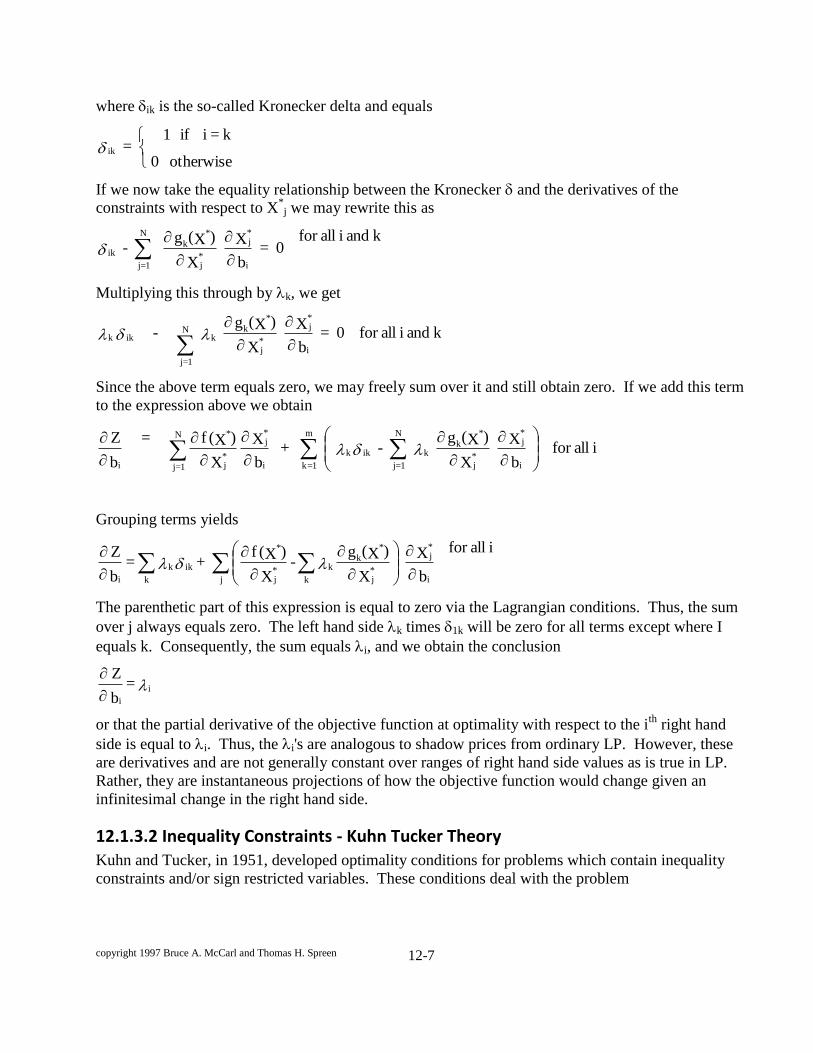
where ik is the so-called Kronecker delta and equals

otherwise 0

k = i if 1 = ik

If we now take the equality relationship between the Kronecker and the derivatives of the

constraints with respect to X*j we may rewrite this as

k and i allfor 0 =

b

X

X

)X(g -

i

*j

*j

*

kN

1j=

ik

Multiplying this through by k, we get

k and i allfor 0 = b

X

X

)X(g -

i

*j

*j

*

kk

N

1j=

ikk

Since the above term equals zero, we may freely sum over it and still obtain zero. If we add this term

to the expression above we obtain

i allfor b

X

X

)X(g - +

b

X

X

)X(f

=

b

Z

i

*j

*j

*

kk

N

1j=

ikk

m

1=ki

*j

*j

*N

1j=i

Grouping terms yields

i allfor

b

X

X

)X(g -

X

)X(f + =

b

Z

i

*j

*j

*

kk

k*j

*

j

ikk

ki

The parenthetic part of this expression is equal to zero via the Lagrangian conditions. Thus, the sum

over j always equals zero. The left hand side k times 1k will be zero for all terms except where I

equals k. Consequently, the sum equals i, and we obtain the conclusion

i

i

= b

Z

or that the partial derivative of the objective function at optimality with respect to the ith

right hand

side is equal to i. Thus, the i's are analogous to shadow prices from ordinary LP. However, these

are derivatives and are not generally constant over ranges of right hand side values as is true in LP.

Rather, they are instantaneous projections of how the objective function would change given an

infinitesimal change in the right hand side.

12.1.3.2 Inequality Constraints - Kuhn Tucker Theory Kuhn and Tucker, in 1951, developed optimality conditions for problems which contain inequality

constraints and/or sign restricted variables. These conditions deal with the problem


0 X

b g(X) .t.s

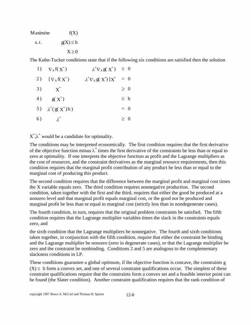
f(X) Maximixe

The Kuhn-Tucker conditions state that if the following six conditions are satisfied then the solution

0 ) 6

0 = ) b) X g( ( ) 5

b ) X g( ) 4

0 X ) 3

0 = X] )X g( ) X f( [ ) 2

0 ) X g( ) X f( ) 1

*

**

*

*

**X

**X

*X

**X

X*,

* would be a candidate for optimality.

The conditions may be interpreted economically. The first condition requires that the first derivative

of the objective function minus * times the first derivative of the constraints be less than or equal to

zero at optimality. If one interprets the objective function as profit and the Lagrange multipliers as

the cost of resources, and the constraint derivatives as the marginal resource requirements, then this

condition requires that the marginal profit contribution of any product be less than or equal to the

marginal cost of producing this product.

The second condition requires that the difference between the marginal profit and marginal cost times

the X variable equals zero. The third condition requires nonnegative production. The second

condition, taken together with the first and the third, requires that either the good be produced at a

nonzero level and that marginal profit equals marginal cost, or the good not be produced and

marginal profit be less than or equal to marginal cost (strictly less than in nondegenerate cases).

The fourth condition, in turn, requires that the original problem constraints be satisfied. The fifth

condition requires that the Lagrange multiplier variables times the slack in the constraints equals

zero, and

the sixth condition that the Lagrange multipliers be nonnegative. The fourth and sixth conditions

taken together, in conjunction with the fifth condition, require that either the constraint be binding

and the Lagrange multiplier be nonzero (zero in degenerate cases), or that the Lagrange multiplier be

zero and the constraint be nonbinding. Conditions 2 and 5 are analogous to the complementary

slackness conditions in LP.

These conditions guarantee a global optimum, if the objective function is concave, the constraints g

(X) b form a convex set, and one of several constraint qualifications occur. The simplest of these

constraint qualifications require that the constraints form a convex set and a feasible interior point can

be found (the Slater condition). Another constraint qualification requires that the rank condition of


the Jacobian be satisfied. There are other forms of constraint qualifications as reviewed in Bazaraa

and Shetty; Gould and Tolle; and Peterson.

12.1.3.2.1 Example 1

0 X

b AX .t.s

CX Maximize

Consider the LP problem

The Kuhn-Tucker conditions of this problem are

0 ) 6

0 = ) b - AX ( ) 5

b AX ) 4

0 X ) 3

0 = X)A - C ( ) 2

0 A - C ) 1

*

**

*

*

**

*

These Kuhn-Tucker conditions are equivalent to the optimality conditions of the LP problem and

show that the Kuhn-Tucker theory is simply a superset of LP theory and LP duality theory as the 's

in the Kuhn-Tucker problem are equivalent to the LP dual variables.

12.1.3.2.2 Example 2

The Kuhn-Tucker theory has also been applied to quadratic programming problems. A

quadratic problem is

0 X

b AX .t.s

QXX2/1 - CX Maximize

and its Kuhn-Tucker conditions are

0)6

0)()5

)4

0)3

0)()2

0)1

*

*

*

*

bXA

bXA

X

XAQXC

AQXC


These Kuhn-Tucker conditions are close to a linear system of equations. If one disregards equations

(2) and (5) the system is linear. These Kuhn-Tucker conditions have provided the basic equations

that specialized quadratic programming algorithms (e.g. Wolfe) attempt to solve.

12.1.4 Usage of Optimality Conditions

Optimality conditions have been used in mathematical programming for three purposes. The first and

least used purpose is to solve numerical problems. Not many modelers check second derivatives or

attempt to solve such things as the Kuhn-Tucker conditions directly. Rather, the more common

usages of the optimality conditions are to characterize optimal solutions analytically, as is very

commonly done in economics, or to provide the conditions that an algorithm attempts to achieve as in

the Wolfe algorithm in quadratic programming.

12.2 Notes on Solution of Nonlinear Programming Models Three general approaches have been used to solve nonlinear models. Problems have been

approximated by a linear model and the resulting model solved via the simplex method as in the

approximations chapter. Second, special problem structures (most notably those with a quadratic

objective function and linear constraints) have been solved with customized algorithms. Third,

general nonlinear programming algorithms such as MINOS within GAMS have been used.

A popular way of solving nonlinear programming problems is the "gradient" method (Lasdon and

Waren, Waren and Lasdon). One of the popular gradient algorithms was developed by Murtaugh

and Saunders (1987) and implemented in MINOS (which is the common GAMS nonlinear solver).

That method solves the problem

Min F(X) = f(XN) + CX

L

s.t. AX b

X 0.

where f(X) is a twice-differentiable convex function. Their approach involves an X vector which

contains variables which only have linear terms, XL, and variables with nonlinear objective terms,

XN.

MINOS first finds a feasible solution to the problem. The usual method employed in LP is to

designate basic variables and non-basic variables which are set equal to zero. However, the optimal

solution to a nonlinear problem is rarely basic. But Murtaugh and Saunders (1987) note that if the

number of nonlinear variables is small, the optimal solution will be "nearly basic"; i.e., the optimal

solution will lie near a basic solution. Thus, they maintain the traditional basic variables as well as

superbasic and traditional non-basic variables. The superbasic variables have nonzero values with

their levels determined by the first order conditions on those variables.

Given a current solution to the problem, X0, MINOS seeks to improve the objective function value.

The algorithm uses the gradient to determine the direction of change, thus GAMS automatically takes

derivatives and passes them to MINOS. The algorithm proceeds until the reduced gradient of the

objective function, in the space determined by the active constraints, is zero. MINOS can also solve

problems with nonlinear constraints. See Gill, Murry and Wright for discussion.


12.3 Expressing Nonlinear Programs in Conjunction with GAMS The solution of nonlinear programming problems in GAMS is a simple extension of the solution of

linear programming problems in GAMS. One ordinarily has to do two things. First, one specifies the

model using nonlinear expressions, and second the solve statement is altered so a nonlinear solver is

used. In addition, it is desirable to specify an initial starting point and that the problem be well

scaled.

An example quadratic programming problem is as follows:

0Q,Q

0QQ

0.1QQ0.15Q6QMax

sd

sd

2

ssdd

This problem is explained in the Price Endogenous modeling chapter and is only presented here for

illustrative purposes. The GAMS formulation is listed in Table 12.1 and is called TABLE12.1 on the

associated disk. The solution to this model as presented in Table 12.2 reveals shadow prices as well

as optimal variable values and reduced costs. The SOLVE statement (line 34) uses the phrase

"USING NLP" which signifies using nonlinear programming. Obviously users must have a license to

a nonlinear programming algorithm such as MINOS to do this. Also, the objective function is

specified as a nonlinear model in lines 26-28.

Finally a caution is also in order. Modelers should avoid nonlinear terms in equations to the extent

possible (excepting in the equation expressing a nonlinear objective function). It is much more

difficult for nonlinear solvers, like MINOS, to deal with nonlinear constraints.


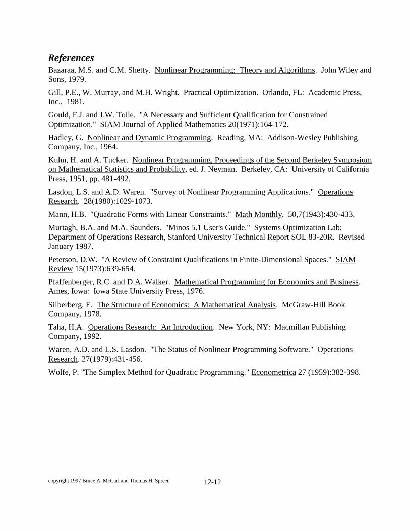
References Bazaraa, M.S. and C.M. Shetty. Nonlinear Programming: Theory and Algorithms. John Wiley and

Sons, 1979.

Gill, P.E., W. Murray, and M.H. Wright. Practical Optimization. Orlando, FL: Academic Press,

Inc., 1981.

Gould, F.J. and J.W. Tolle. "A Necessary and Sufficient Qualification for Constrained

Optimization." SIAM Journal of Applied Mathematics 20(1971):164-172.

Hadley, G. Nonlinear and Dynamic Programming. Reading, MA: Addison-Wesley Publishing

Company, Inc., 1964.

Kuhn, H. and A. Tucker. Nonlinear Programming, Proceedings of the Second Berkeley Symposium

on Mathematical Statistics and Probability, ed. J. Neyman. Berkeley, CA: University of California

Press, 1951, pp. 481-492.

Lasdon, L.S. and A.D. Waren. "Survey of Nonlinear Programming Applications." Operations

Research. 28(1980):1029-1073.

Mann, H.B. "Quadratic Forms with Linear Constraints." Math Monthly. 50,7(1943):430-433.

Murtagh, B.A. and M.A. Saunders. "Minos 5.1 User's Guide." Systems Optimization Lab;

Department of Operations Research, Stanford University Technical Report SOL 83-20R. Revised

January 1987.

Peterson, D.W. "A Review of Constraint Qualifications in Finite-Dimensional Spaces." SIAM

Review 15(1973):639-654.

Pfaffenberger, R.C. and D.A. Walker. Mathematical Programming for Economics and Business.

Ames, Iowa: Iowa State University Press, 1976.

Silberberg, E. The Structure of Economics: A Mathematical Analysis. McGraw-Hill Book

Company, 1978.

Taha, H.A. Operations Research: An Introduction. New York, NY: Macmillan Publishing

Company, 1992.

Waren, A.D. and L.S. Lasdon. "The Status of Nonlinear Programming Software." Operations

Research. 27(1979):431-456.

Wolfe, P. "The Simplex Method for Quadratic Programming." Econometrica 27 (1959):382-398.


Table 12.1. GAMS Formulation of Nonlinear Programming Example

2

4 OPTION LIMCOL = 0;

5 OPTION LIMROW = 0;

6

7 SETS CURVEPARM CURVE PARAMETERS /INTERCEPT,SLOPE/

8 CURVES TYPES OF CURVES /DEMAND,SUPPLY/

9

10 TABLE DATA(CURVES,CURVEPARM) SUPPLY DEMAND DATA

11

12 INTERCEPT SLOPE

13 DEMAND 6 -0.30

14 SUPPLY 1 0.20

15

16 PARAMETERS SIGN(CURVES) SIGN ON CURVES IN OBJECTIVE FUNCTION

17 /SUPPLY -1, DEMAND 1/

18

19 POSITIVE VARIABLES QUANTITY(CURVES) ACTIVITY LEVEL

20

21 VARIABLES OBJ NUMBER TO BE MAXIMIZED

22

23 EQUATIONS OBJJ OBJECTIVE FUNCTION

24 BALANCE COMMODITY BALANCE;

25

26 OBJJ.. OBJ =E= SUM(CURVES, SIGN(CURVES)*

27 (DATA(CURVES,"INTERCEPT")*QUANTITY(CURVES)

28 +0.5*DATA(CURVES,"SLOPE")*QUANTITY(CURVES)**2)) ;

29

30 BALANCE.. SUM(CURVES, SIGN(CURVES)*QUANTITY(CURVES)) =L= 0 ;

31

32 MODEL PRICEEND /ALL/ ;

33

34 SOLVE PRICEEND USING NLP MAXIMIZING OBJ ;

35

Table 12.2. Solution to Nonlinear Example Model

Variables

Value

Reduced Cost

Equation

Level

Shadow Price

Qd

10

0

Objective function

25

-

Qs

10

0

Constraint

0

3

CHAPTER XII: NONLINEAR OPTIMIZATION CONDITIONS

Documents

Transcript of CHAPTER XII: NONLINEAR OPTIMIZATION CONDITIONS