No Slide Titleweb.engr.illinois.edu/~khashab2/files/2015_cs446_machine_learning/... · There will...
119
NEURAL NETWORKS CS446 -FALL ‘15 Administration HW4 will be out next week! Midterm is close! Come to sections with questions 1
Transcript of No Slide Titleweb.engr.illinois.edu/~khashab2/files/2015_cs446_machine_learning/... · There will...

NEURAL NETWORKS CS446 -FALL ‘15
Administration
HW4 will be out next week!
Midterm is close! Come to sections with questions
1

NEURAL NETWORKS CS446 -FALL ‘15
Administration
HW4 will be out next week!
Midterm is close! Come to sections with questions
1
Questions

NEURAL NETWORKS CS446 -FALL ‘15
Administration
HW4 will be out next week!
Midterm is close! Come to sections with questions
Projects proposals are due on Friday 10/16/15
1
Questions

NEURAL NETWORKS CS446 -FALL ‘15
Projects
Projects proposals are due on Friday 10/16/15 Within a week we will give you an approval to continue with your project along with comments and/or a request to modify/augment/do a different project. There will also be a mechanism for peer comments. We allow team projects – a team can be up to 3 people. Please start thinking and working on the project. Your proposal is limited to 1-2 pages, but needs to include references and, ideally, some of the ideas you have developed in the direction of the project (maybe even some preliminary results). Any project that has a significant Machine Learning component is good. You can do experimental work, theoretical work, a combination of both or a critical survey of results in some specialized topic. The work has to include some reading. Even if you do not do a survey, you must read (at least) two related papers or book chapters and relate your work to it. Originality is not mandatory but is encouraged. Try to make it interesting!
2

NEURAL NETWORKS CS446 -FALL ‘15
Neural Networks
3

NEURAL NETWORKS CS446 -FALL ‘15
Neural Networks
Robust approach to approximating real-valued, discrete-valued and vector valued target functions.
Among the most effective general purpose learning method currently known.
3

NEURAL NETWORKS CS446 -FALL ‘15
Neural Networks
Robust approach to approximating real-valued, discrete-valued and vector valued target functions.
Among the most effective general purpose learning method currently known.
Effective especially for complex and hard to interpret input data such as real-world sensory data
The Backpropagation algorithm for neural networks has been shown successful in many practical problems handwritten character recognition, spoken words
recognition, face recognition
3
NEURAL NETWORKS CS446 -FALL ‘15
Neural Networks
N: 𝑋 → 𝑌 = 0,1 𝑛, or {0,1}𝑛 and 𝑌 = 0,1 , {0,1}
4

NEURAL NETWORKS CS446 -FALL ‘15
Neural Networks
0,1 𝑛 0,1 0,1 0,1 0,1 𝑛 𝑛𝑛 0,1 𝑛 , or {0,1} 𝑛 {0,1} {0,1} 𝑛 𝑛𝑛 {0,1} 𝑛 and 𝑌𝑌= 0,1 0,1 0,1 , {0,1}
N:𝑋𝑋→𝑌𝑌 where 𝑋 = 0,1 𝑛, or {0,1}𝑛 and 𝑌 = 0,1 , {0,1}
= 0,1 𝑛, or {0,1}𝑛 and 𝑌 = 0,1 , {0,1}
4
NEURAL NETWORKS CS446 -FALL ‘15
Neural Networks
0,1 𝑛 0,1 0,1 0,1 0,1 𝑛 𝑛𝑛 0,1 𝑛 , or {0,1} 𝑛 {0,1} {0,1} 𝑛 𝑛𝑛 {0,1} 𝑛 and 𝑌𝑌= 0,1 0,1 0,1 , {0,1}
N:𝑋𝑋→𝑌𝑌
NN can be used as an approximation of a target classifier In their general form, NN can approximate any function
4

NEURAL NETWORKS CS446 -FALL ‘15
Neural Networks
0,1 𝑛 0,1 0,1 0,1 0,1 𝑛 𝑛𝑛 0,1 𝑛 , or {0,1} 𝑛 {0,1} {0,1} 𝑛 𝑛𝑛 {0,1} 𝑛 and 𝑌𝑌= 0,1 0,1 0,1 , {0,1}
N:𝑋𝑋→𝑌𝑌
NN can be used as an approximation of a target classifier In their general form, NN can approximate any function
Algorithms exist that can learn a NN representation from labeled training data (e.g., Backpropagation).
4
NEURAL NETWORKS CS446 -FALL ‘15
Multi-Layer Neural Networks
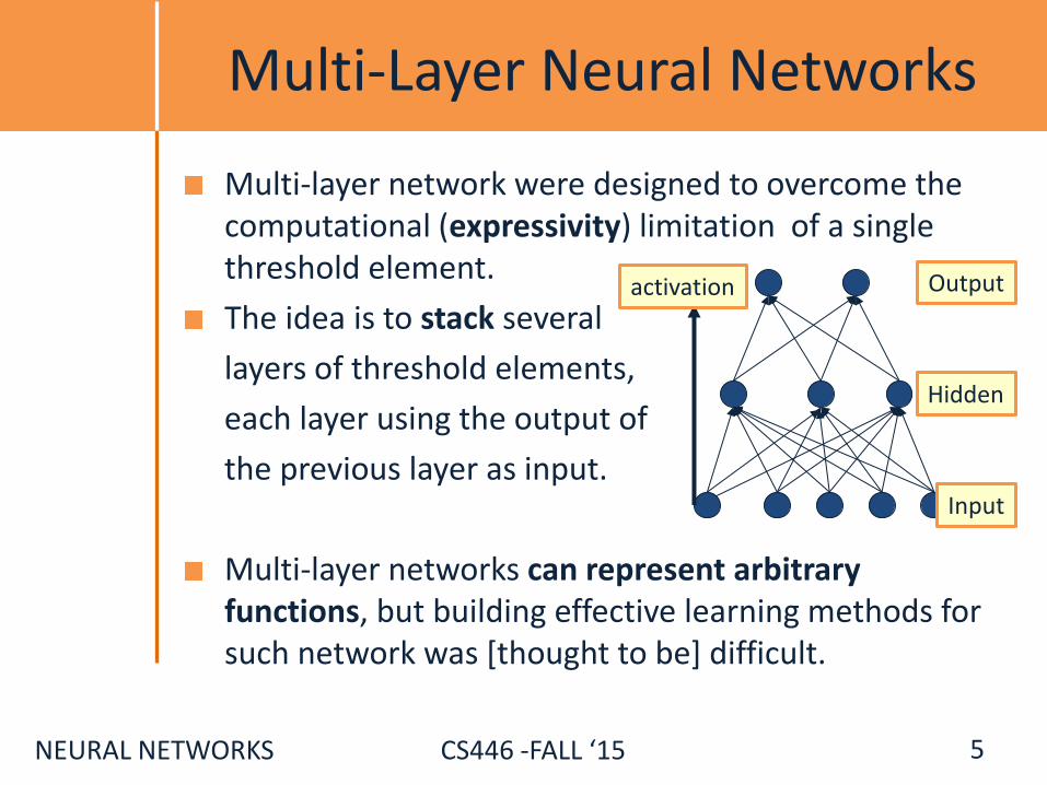
Multi-layer network were designed to overcome the computational (expressivity) limitation of a single threshold element.
The idea is to stack several
layers of threshold elements,
each layer using the output of
the previous layer as input.
Multi-layer networks can represent arbitrary functions, but building effective learning methods for such network was [thought to be] difficult.
5
activation
Input
Hidden
Output

NEURAL NETWORKS CS446 -FALL ‘15
Motivation for Neural Networks
Inspired by biological systems, the best examples we have of robust learning systems Used to model biological systems (so we understand how
they learn)
Massive parallelism that may allow for computational efficiency
6
NEURAL NETWORKS CS446 -FALL ‘15
Motivation for Neural Networks
Inspired by biological systems, the best examples we have of robust learning systems Used to model biological systems (so we understand how
they learn)
Massive parallelism that may allow for computational efficiency
Graceful degradation due to distributed representation that spread the representation of knowledge among the computational units.
Intelligent behavior “emerges” from large number of simple units rather than from explicit symbolically encoded rules.
6
NEURAL NETWORKS CS446 -FALL ‘15
Neural Speed Constraints
Neuron “switching time” is O(milliseconds), compared to nanosecond for transistors. However, biological systems can perform significant cognitive
tasks (vision, language understanding) in fractions of a second.
Even for limited abilities, current AI systems require orders of magnitude more steps.
Human brain has approximately 10^10 neurons, each connected to 10^4; must explore massive parallelism (but there’s more…)
7

NEURAL NETWORKS CS446 -FALL ‘15
Basic Unit in Multi-Layer Neural Network
𝑠𝑠𝑔𝑔𝑛𝑛( 𝑤 𝑤𝑤 𝑤 . 𝑥 𝑥𝑥 𝑥 −𝑇𝑇) are not differentiable, hence unsuitable for gradient descent
𝑤 𝑤𝑤 𝑤 . 𝑥 𝑥𝑥 𝑥 multiple layers of linear functions produce linear functions. We want to represent nonlinear functions.
Threshold units: 𝑜 𝑗 = 𝑗 𝑗 𝑗 = 𝑠𝑔𝑛(𝑤. 𝑥 − 𝑇) are not differentiable, hence unsuitable for gradient descent
Threshold units: 𝑜𝑗 = 𝑠𝑔𝑛(𝑤. 𝑥 − 𝑇) are not
differentiable, hence unsuitable for gradient descent
8
activation
Input
Hidden
Output

NEURAL NETWORKS CS446 -FALL ‘15
Model Neuron (Logistic)
Neuron is modeled by a unit 𝑗 connected by weighted links 𝑤𝑖𝑗 to other units 𝑖.
Use a non-linear, differentiable output function such as the
sigmoid or logistic function
9
𝑜𝑗
𝑥1 𝑥2 𝑥3 𝑥4 𝑥5 𝑥6
𝑥7 𝑤17
𝑤67

NEURAL NETWORKS CS446 -FALL ‘15
Model Neuron (Logistic)
Neuron is modeled by a unit 𝑗 connected by weighted links 𝑤𝑖𝑗 to other units 𝑖.
Use a non-linear, differentiable output function such as the
sigmoid or logistic function
Net input to a unit is defined as:
9
net𝑗 = ∑𝑤𝑖𝑗 . 𝑥𝑖
𝑜𝑗
𝑥1 𝑥2 𝑥3 𝑥4 𝑥5 𝑥6
𝑥7 𝑤17
𝑤67

NEURAL NETWORKS CS446 -FALL ‘15
Model Neuron (Logistic)
Neuron is modeled by a unit 𝑗 connected by weighted links 𝑤𝑖𝑗 to other units 𝑖.
Use a non-linear, differentiable output function such as the
sigmoid or logistic function
Net input to a unit is defined as:
Output of a unit is defined as:
9
net𝑗 = ∑𝑤𝑖𝑗 . 𝑥𝑖
𝑜𝑗 =1
1 + exp −(net𝑗 − 𝑇𝑗)
𝑜𝑗
𝑥1 𝑥2 𝑥3 𝑥4 𝑥5 𝑥6
𝑥7 𝑤17
𝑤67
The parameters so far?

NEURAL NETWORKS CS446 -FALL ‘15
Model Neuron (Logistic)
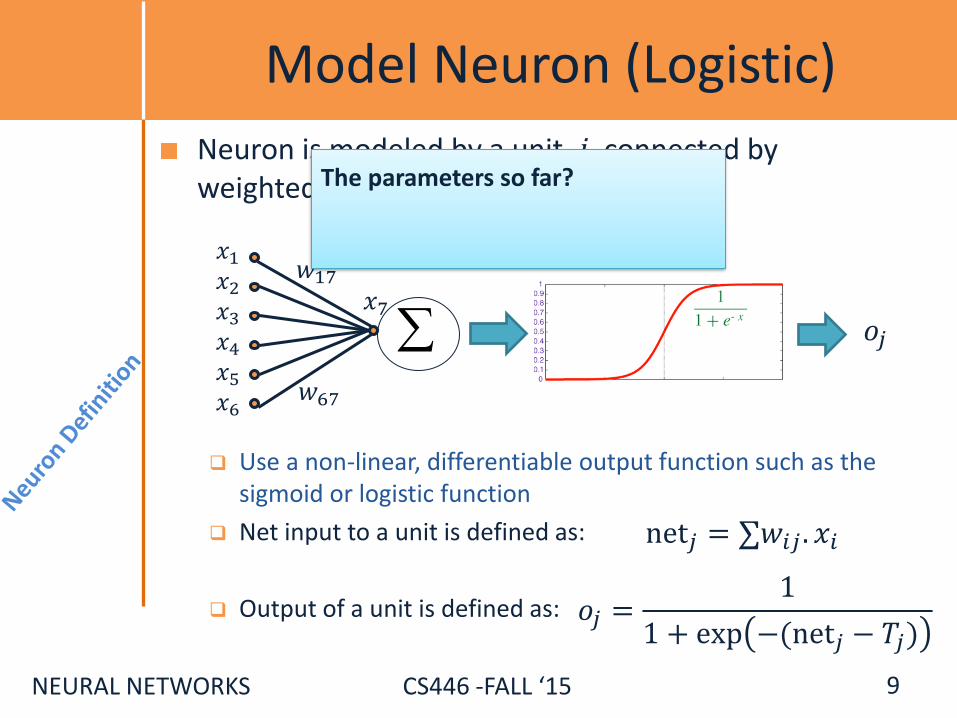
Neuron is modeled by a unit 𝑗 connected by weighted links 𝑤𝑖𝑗 to other units 𝑖.
Use a non-linear, differentiable output function such as the
sigmoid or logistic function
Net input to a unit is defined as:
Output of a unit is defined as:
9
net𝑗 = ∑𝑤𝑖𝑗 . 𝑥𝑖
𝑜𝑗 =1
1 + exp −(net𝑗 − 𝑇𝑗)
𝑜𝑗
𝑥1 𝑥2 𝑥3 𝑥4 𝑥5 𝑥6
𝑥7 𝑤17
𝑤67
The parameters so far? The set of connectThe threshold value: 𝑇 𝑗 𝑗 𝑗 𝑗 𝑖𝑗 𝑗 𝑖𝑗 The threshold value: 𝑇𝑗

NEURAL NETWORKS CS446 -FALL ‘15
Neural Computation
McCollough and Pitts (1943) showed how linear threshold units can be used to compute logical functions
Can build basic logic gates AND:
OR:
NOT: One input =1, the input to be inverted have negative weight
10

NEURAL NETWORKS CS446 -FALL ‘15
Neural Computation
McCollough and Pitts (1943) showed how linear threshold units can be used to compute logical functions
Can build basic logic gates AND:
OR:
NOT: One input =1, the input to be inverted have negative weight
10
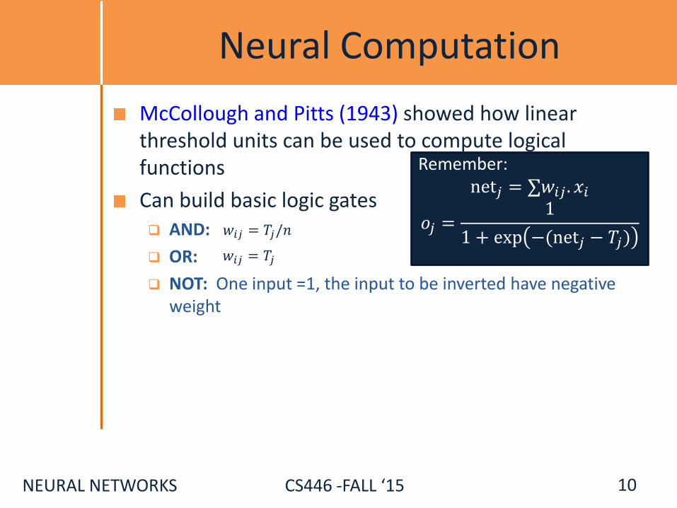
Remember: net𝑗 = ∑𝑤𝑖𝑗 . 𝑥𝑖
𝑜𝑗 =1
1 + exp −(net𝑗 − 𝑇𝑗)

NEURAL NETWORKS CS446 -FALL ‘15
Neural Computation
McCollough and Pitts (1943) showed how linear threshold units can be used to compute logical functions
Can build basic logic gates AND:
OR:
NOT: One input =1, the input to be inverted have negative weight
10
Remember: net𝑗 = ∑𝑤𝑖𝑗 . 𝑥𝑖
𝑜𝑗 =1
1 + exp −(net𝑗 − 𝑇𝑗)
𝑤𝑖𝑗 = 𝑇𝑗/𝑛
𝑤𝑖𝑗 = 𝑇𝑗

NEURAL NETWORKS CS446 -FALL ‘15
Neural Computation
McCollough and Pitts (1943) showed how linear threshold units can be used to compute logical functions
Can build basic logic gates AND:
OR:
NOT: One input =1, the input to be inverted have negative weight
Can build arbitrary logic circuits, finite-state machines and computers given these basis gates.
Can specify any Boolean function using two layer network (w/ negation) DNF and CNF are universal representations
10
Remember: net𝑗 = ∑𝑤𝑖𝑗 . 𝑥𝑖
𝑜𝑗 =1
1 + exp −(net𝑗 − 𝑇𝑗)
𝑤𝑖𝑗 = 𝑇𝑗/𝑛
𝑤𝑖𝑗 = 𝑇𝑗

NEURAL NETWORKS CS446 -FALL ‘15
Learning Rules
Hebb (1949) suggested that if two units are both active (firing) then the weights between them should increase: 𝑤𝑖𝑗 = 𝑤𝑖𝑗 + 𝑅𝑜𝑖𝑜𝑗
𝑅 and is a constant called the learning rate
Supported by physiological evidence
11

NEURAL NETWORKS CS446 -FALL ‘15
Learning Rules
Hebb (1949) suggested that if two units are both active (firing) then the weights between them should increase: 𝑤𝑖𝑗 = 𝑤𝑖𝑗 + 𝑅𝑜𝑖𝑜𝑗
𝑅 and is a constant called the learning rate
Supported by physiological evidence
Rosenblatt (1959) suggested that when a target output value is provided for a single neuron with fixed input, it can incrementally change weights and learn to produce the output using the Perceptron learning rule. assumes binary output units; single linear threshold unit
11

NEURAL NETWORKS CS446 -FALL ‘15
Perceptron Learning Rule
Given:
the target output for the output unit is 𝑡𝑗
the input the neuron sees is 𝑥𝑖
the output it produces is 𝑜𝑗
Update weights according to 𝑤𝑖𝑗 ← 𝑤𝑖𝑗 + 𝑅 𝑡𝑗 − 𝑜𝑗 𝑥𝑖
12
𝑇𝑗
𝑜𝑗
𝑥1 𝑥2 𝑥3 𝑥4 𝑥5 𝑥6
𝑥7 𝑤17
𝑤67

NEURAL NETWORKS CS446 -FALL ‘15
Perceptron Learning Rule
Given:
the target output for the output unit is 𝑡𝑗
the input the neuron sees is 𝑥𝑖
the output it produces is 𝑜𝑗
Update weights according to 𝑤𝑖𝑗 ← 𝑤𝑖𝑗 + 𝑅 𝑡𝑗 − 𝑜𝑗 𝑥𝑖
If output is correct, don’t change the weights
12
𝑇𝑗
𝑜𝑗
𝑥1 𝑥2 𝑥3 𝑥4 𝑥5 𝑥6
𝑥7 𝑤17
𝑤67

NEURAL NETWORKS CS446 -FALL ‘15
Perceptron Learning Rule
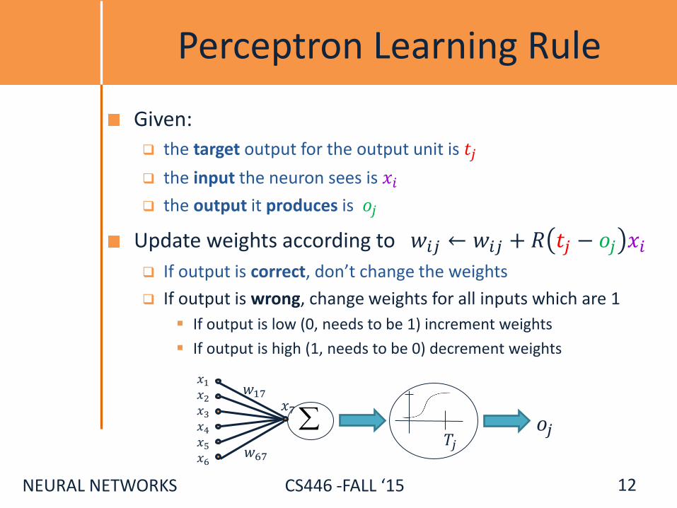
Given:
the target output for the output unit is 𝑡𝑗
the input the neuron sees is 𝑥𝑖
the output it produces is 𝑜𝑗
Update weights according to 𝑤𝑖𝑗 ← 𝑤𝑖𝑗 + 𝑅 𝑡𝑗 − 𝑜𝑗 𝑥𝑖
If output is correct, don’t change the weights
If output is wrong, change weights for all inputs which are 1
12
𝑇𝑗
𝑜𝑗
𝑥1 𝑥2 𝑥3 𝑥4 𝑥5 𝑥6
𝑥7 𝑤17
𝑤67

NEURAL NETWORKS CS446 -FALL ‘15
Perceptron Learning Rule
Given:
the target output for the output unit is 𝑡𝑗
the input the neuron sees is 𝑥𝑖
the output it produces is 𝑜𝑗
Update weights according to 𝑤𝑖𝑗 ← 𝑤𝑖𝑗 + 𝑅 𝑡𝑗 − 𝑜𝑗 𝑥𝑖
If output is correct, don’t change the weights
If output is wrong, change weights for all inputs which are 1
If output is low (0, needs to be 1) increment weights
12
𝑇𝑗
𝑜𝑗
𝑥1 𝑥2 𝑥3 𝑥4 𝑥5 𝑥6
𝑥7 𝑤17
𝑤67
NEURAL NETWORKS CS446 -FALL ‘15
Perceptron Learning Rule
Given:
the target output for the output unit is 𝑡𝑗
the input the neuron sees is 𝑥𝑖
the output it produces is 𝑜𝑗
Update weights according to 𝑤𝑖𝑗 ← 𝑤𝑖𝑗 + 𝑅 𝑡𝑗 − 𝑜𝑗 𝑥𝑖
If output is correct, don’t change the weights
If output is wrong, change weights for all inputs which are 1
If output is low (0, needs to be 1) increment weights
If output is high (1, needs to be 0) decrement weights
12
𝑇𝑗
𝑜𝑗
𝑥1 𝑥2 𝑥3 𝑥4 𝑥5 𝑥6
𝑥7 𝑤17
𝑤67
NEURAL NETWORKS CS446 -FALL ‘15
Perceptron Learning Algorithm
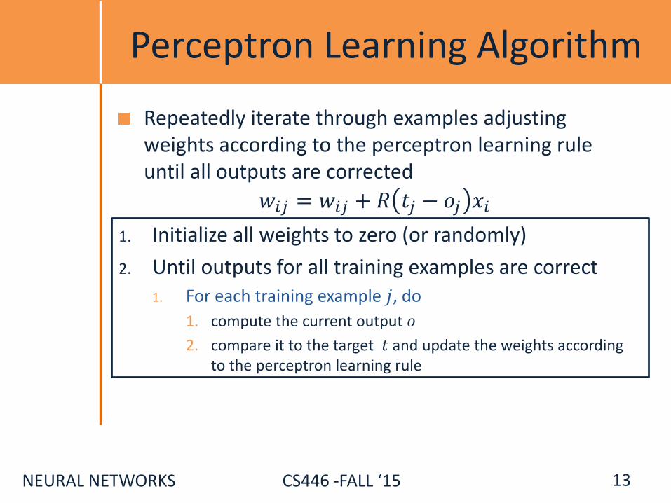
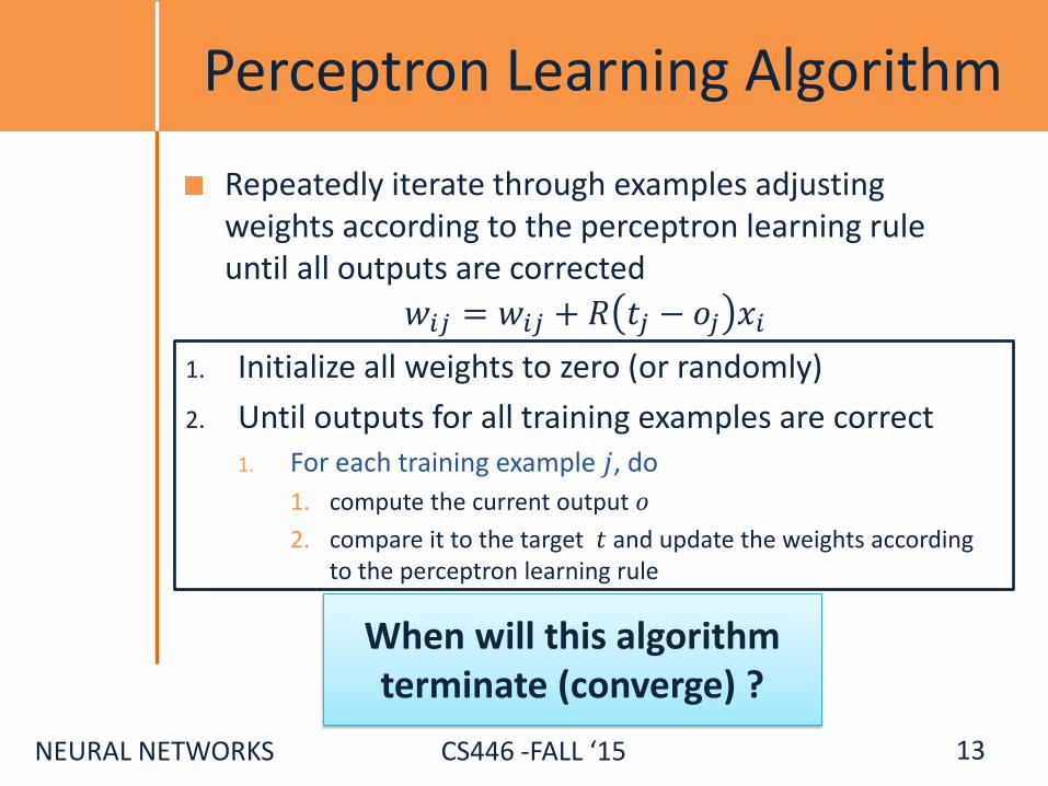
Repeatedly iterate through examples adjusting weights according to the perceptron learning rule until all outputs are corrected
𝑤𝑖𝑗 = 𝑤𝑖𝑗 + 𝑅 𝑡𝑗 − 𝑜𝑗 𝑥𝑖
1. Initialize all weights to zero (or randomly)
2. Until outputs for all training examples are correct 1. For each training example 𝑗, do
1. compute the current output 𝑜
2. compare it to the target 𝑡 and update the weights according to the perceptron learning rule
13
NEURAL NETWORKS CS446 -FALL ‘15
Perceptron Learning Algorithm
Repeatedly iterate through examples adjusting weights according to the perceptron learning rule until all outputs are corrected
𝑤𝑖𝑗 = 𝑤𝑖𝑗 + 𝑅 𝑡𝑗 − 𝑜𝑗 𝑥𝑖
1. Initialize all weights to zero (or randomly)
2. Until outputs for all training examples are correct 1. For each training example 𝑗, do
1. compute the current output 𝑜
2. compare it to the target 𝑡 and update the weights according to the perceptron learning rule
13
When will this algorithm terminate (converge) ?

NEURAL NETWORKS CS446 -FALL ‘15
Perceptron Convergence
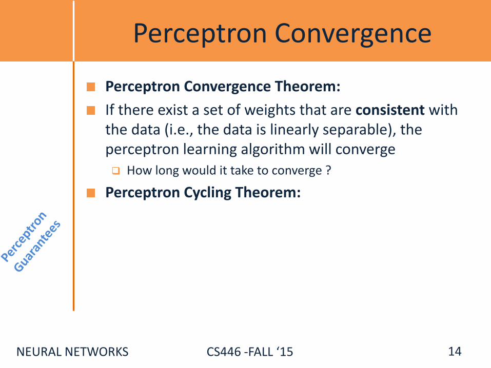
Perceptron Convergence Theorem:
14

NEURAL NETWORKS CS446 -FALL ‘15
Perceptron Convergence
Perceptron Convergence Theorem:
If there exist a set of weights that are consistent with the data (i.e., the data is linearly separable), the perceptron learning algorithm will converge
14

NEURAL NETWORKS CS446 -FALL ‘15
Perceptron Convergence
Perceptron Convergence Theorem:
If there exist a set of weights that are consistent with the data (i.e., the data is linearly separable), the perceptron learning algorithm will converge How long would it take to converge ?
14
NEURAL NETWORKS CS446 -FALL ‘15
Perceptron Convergence
Perceptron Convergence Theorem:
If there exist a set of weights that are consistent with the data (i.e., the data is linearly separable), the perceptron learning algorithm will converge How long would it take to converge ?
Perceptron Cycling Theorem:
14

NEURAL NETWORKS CS446 -FALL ‘15
Perceptron Convergence
Perceptron Convergence Theorem:
If there exist a set of weights that are consistent with the data (i.e., the data is linearly separable), the perceptron learning algorithm will converge How long would it take to converge ?
Perceptron Cycling Theorem:
If the training data is not linearly separable the perceptron learning algorithm will eventually repeat the same set of weights and therefore enter an infinite loop.
14

NEURAL NETWORKS CS446 -FALL ‘15
Perceptron Convergence
Perceptron Convergence Theorem:
If there exist a set of weights that are consistent with the data (i.e., the data is linearly separable), the perceptron learning algorithm will converge How long would it take to converge ?
Perceptron Cycling Theorem:
If the training data is not linearly separable the perceptron learning algorithm will eventually repeat the same set of weights and therefore enter an infinite loop. How to provide robustness, more expressivity ?
14

NEURAL NETWORKS CS446 -FALL ‘15
Perceptron Learnability
Obviously cannot learn what it cannot represent Only linearly separable functions
15

NEURAL NETWORKS CS446 -FALL ‘15
Perceptron Learnability
Obviously cannot learn what it cannot represent Only linearly separable functions
Minsky and Papert (1969) wrote an influential book in which they demonstrate the representational limitations of Perceptron Parity functions cannot be learned (generalization of XOR)
In visual pattern recognition, if patterns are represented using local features, perceptron cannot represent properties like Symmetry, Connectivity
These observations discouraged research on neural network for years.
But, Rosenblatt (1959) asked: “What pattern recognition problems can be transformed so as to become linearly separable”
15

NEURAL NETWORKS CS446 -FALL ‘15
16
(x1 x2) v (x3 x4) y1 y2

NEURAL NETWORKS CS446 -FALL ‘15
Widrow-Hoff Rule
This incremental update rule provides an approximation to the goal: Find the best linear approximation of the data
𝐸𝑟𝑟 𝑤 𝑗 =1
2 𝑡𝑑 − 𝑜𝑑
2
𝑑∈𝐷
where:
𝑜𝑑 = 𝑤𝑖𝑗 . 𝑥𝑖 =
𝑖
𝑤 𝑗 . 𝑥
output of linear unit on example d
𝑡𝑑 = Target output for example d
17

NEURAL NETWORKS CS446 -FALL ‘15
Gradient Descent
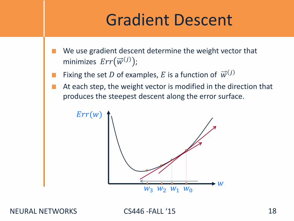
We use gradient descent determine the weight vector that
minimizes 𝐸𝑟𝑟 𝑤 𝑗 ;
Fixing the set 𝐷 of examples, 𝐸 is a function of 𝑤 𝑗
At each step, the weight vector is modified in the direction that produces the steepest descent along the error surface.
18
𝐸𝑟𝑟(𝑤)
𝑤 𝑤3 𝑤2 𝑤1 𝑤0

NEURAL NETWORKS CS446 -FALL ‘15
Gradient Descent
We use gradient descent determine the weight vector that
minimizes 𝐸𝑟𝑟 𝑤 𝑗 ;
Fixing the set 𝐷 of examples, 𝐸 is a function of 𝑤 𝑗
At each step, the weight vector is modified in the direction that produces the steepest descent along the error surface.
18
𝐸𝑟𝑟(𝑤)
𝑤 𝑤3 𝑤2 𝑤1 𝑤0

NEURAL NETWORKS CS446 -FALL ‘15
Gradient Descent
To find the best direction in the feature space we compute the gradient of 𝐸 with respect to each of the components of 𝑤
𝛻𝐸 𝑤 =𝜕𝐸
𝜕𝑤1,𝜕𝐸
𝜕𝑤2, … ,𝜕𝐸
𝜕𝑤𝑛
This vector specifies the direction the produces the steepest increase in 𝐸;
in the direction of −𝛻𝐸 𝑤 𝑤 ← 𝑤 + Δ𝑤
Where: Δ𝑤 = −R 𝛻𝐸 𝑤
19

NEURAL NETWORKS CS446 -FALL ‘15
Gradient Descent
𝑤 𝑤𝑤 𝑤 =−R 𝛻𝛻𝐸𝐸 𝑤 𝑤 𝑤𝑤 𝑤 𝑤
𝑤 𝑤𝑤 𝑤 +Δ 𝑤 𝑤𝑤 𝑤
in the direction of −𝛻𝛻𝐸𝐸 𝑤 𝑤 𝑤𝑤 𝑤 𝑤
To find the best direction in the feature space we compute the gradient of 𝐸 with respect to each of the components of 𝑤
𝛻𝐸 𝑤 =𝜕𝐸
𝜕𝑤1,𝜕𝐸
𝜕𝑤2, … ,𝜕𝐸
𝜕𝑤𝑛
This vector specifies the direction the produces the steepest increase in 𝐸;
Δ𝑤 = −R 𝛻𝐸 𝑤
Where: Δ𝑤 = −R 𝛻𝐸 𝑤
19

NEURAL NETWORKS CS446 -FALL ‘15
Gradient Descent – LMS
We have: 𝐸𝑟𝑟 𝑤 𝑗 =1
2∑ 𝑡𝑑 − 𝑜𝑑
2𝑑∈𝐷
Therefore:
20
=𝜕
𝜕𝑤𝑖
1
2 𝑡𝑑 − 𝑜𝑑
2
𝑑∈𝐷
𝜕𝐸
𝜕𝑤𝑖

NEURAL NETWORKS CS446 -FALL ‘15
Gradient Descent – LMS
We have: 𝐸𝑟𝑟 𝑤 𝑗 =1
2∑ 𝑡𝑑 − 𝑜𝑑
2𝑑∈𝐷
Therefore:
20
=𝜕
𝜕𝑤𝑖
1
2 𝑡𝑑 − 𝑜𝑑
2
𝑑∈𝐷
=1
2 𝜕
𝜕𝑤𝑖𝑡𝑑 − 𝑜𝑑
2
𝑑∈𝐷
= 𝜕𝐸
𝜕𝑤𝑖

NEURAL NETWORKS CS446 -FALL ‘15
Gradient Descent – LMS
We have: 𝐸𝑟𝑟 𝑤 𝑗 =1
2∑ 𝑡𝑑 − 𝑜𝑑
2𝑑∈𝐷
Therefore:
20
=𝜕
𝜕𝑤𝑖
1
2 𝑡𝑑 − 𝑜𝑑
2
𝑑∈𝐷
=1
2 𝜕
𝜕𝑤𝑖𝑡𝑑 − 𝑜𝑑
2
𝑑∈𝐷
=
=1
2 𝑡𝑑 − 𝑜𝑑
𝜕
𝜕𝑤𝑖𝑡𝑑 −𝑤. 𝑥 𝑑 =
𝑑∈𝐷
𝜕𝐸
𝜕𝑤𝑖

NEURAL NETWORKS CS446 -FALL ‘15
Gradient Descent – LMS
We have: 𝐸𝑟𝑟 𝑤 𝑗 =1
2∑ 𝑡𝑑 − 𝑜𝑑
2𝑑∈𝐷
Therefore:
20
=𝜕
𝜕𝑤𝑖
1
2 𝑡𝑑 − 𝑜𝑑
2
𝑑∈𝐷
=1
2 𝜕
𝜕𝑤𝑖𝑡𝑑 − 𝑜𝑑
2
𝑑∈𝐷
=
=1
2 𝑡𝑑 − 𝑜𝑑
𝜕
𝜕𝑤𝑖𝑡𝑑 −𝑤. 𝑥 𝑑 =
𝑑∈𝐷
= 𝑡𝑑 − 𝑜𝑑 −𝑥𝑖𝑑𝑑∈𝐷
𝜕𝐸
𝜕𝑤𝑖
𝑤 = [𝑤1, … , 𝑤𝑛] 𝑥 𝑑 = [𝑥1𝑑 , … , 𝑥𝑛𝑑]

NEURAL NETWORKS CS446 -FALL ‘15
Gradient Descent – LMS
Weight update rule: Δ𝑤𝑖 = 𝑅∑ 𝑡𝑑 − 𝑜𝑑 𝑥 𝑖𝑑𝑑∈𝐷
Gradient descent algorithm for training linear units: 1. Start with an initial random weight vector
2. For every example d with target value 𝑡𝑑:
1. Evaluate the linear unit 𝑜𝑑 = ∑ 𝑤𝑖 . 𝑥𝑑 =𝑖 𝑤 𝑗 . 𝑥 𝑑
3. update 𝑤 by adding Δ𝑤𝑖 to each component
4. Continue until 𝐸 below some threshold
21

NEURAL NETWORKS CS446 -FALL ‘15
Gradient Descent – LMS
Weight update rule: Δ𝑤𝑖 = 𝑅∑ 𝑡𝑑 − 𝑜𝑑 𝑥 𝑖𝑑𝑑∈𝐷
Gradient descent algorithm for training linear units: 1. Start with an initial random weight vector
2. For every example d with target value 𝑡𝑑:
1. Evaluate the linear unit 𝑜𝑑 = ∑ 𝑤𝑖 . 𝑥𝑑 =𝑖 𝑤 𝑗 . 𝑥 𝑑
3. update 𝑤 by adding Δ𝑤𝑖 to each component
4. Continue until 𝐸 below some threshold
Because the surface contains only a single global minimum the algorithm will converge to a weight vector with minimum error, regardless of whether the training examples are linearly separable
21

NEURAL NETWORKS CS446 -FALL ‘15
Gradient Descent – LMS
Weight update rule: Δ = 𝑅
22

NEURAL NETWORKS CS446 -FALL ‘15
Gradient Descent – LMS
Weight update rule: Δ = 𝑅
In general does not converge to global minimum
Robbins-Monro: Decreasing 𝑅 with time, guarantees convergence.
22

NEURAL NETWORKS CS446 -FALL ‘15
Summary: Single Layer Network
Variety of update rules Multiplicative
Additive
Batch and incremental algorithms
Various convergence and efficiency conditions
There are other ways to learn linear functions Linear Programming (general purpose)
Probabilistic Classifiers ( some assumption)
Although simple and restrictive -- linear predictors perform very well on many realistic problems
However, the representational restriction is limiting in many applications
23

NEURAL NETWORKS CS446 -FALL ‘15
Learning with a Multi-Layer Perceptron
It’s easy to learn the top layer – it’s just a linear unit.
Given feedback (truth) at the top layer, and the activation at the layer below it, you can use the Perceptron update rule (more generally, gradient descent) to updated these weights.
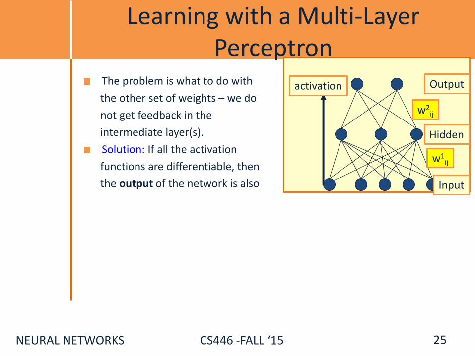
The problem is what to do with
the other set of weights – we do
not get feedback in the
intermediate layer(s).
24
activation
Input
Hidden
Output
w2ij
w1ij

NEURAL NETWORKS CS446 -FALL ‘15
Learning with a Multi-Layer Perceptron
The problem is what to do with
the other set of weights – we do
not get feedback in the
intermediate layer(s).
25
activation
Input
Hidden
Output
w2ij
w1ij

NEURAL NETWORKS CS446 -FALL ‘15
Learning with a Multi-Layer Perceptron
The problem is what to do with
the other set of weights – we do
not get feedback in the
intermediate layer(s).
Solution: If all the activation
25
activation
Input
Hidden
Output
w2ij
w1ij

NEURAL NETWORKS CS446 -FALL ‘15
Learning with a Multi-Layer Perceptron
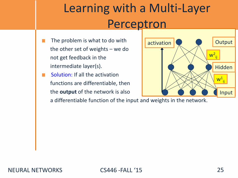
The problem is what to do with
the other set of weights – we do
not get feedback in the
intermediate layer(s).
Solution: If all the activation
functions are differentiable, then
25
activation
Input
Hidden
Output
w2ij
w1ij
NEURAL NETWORKS CS446 -FALL ‘15
Learning with a Multi-Layer Perceptron
The problem is what to do with
the other set of weights – we do
not get feedback in the
intermediate layer(s).
Solution: If all the activation
functions are differentiable, then
the output of the network is also
a differentiable function of the input and weights in the network.
25
activation
Input
Hidden
Output
w2ij
w1ij
NEURAL NETWORKS CS446 -FALL ‘15
Learning with a Multi-Layer Perceptron
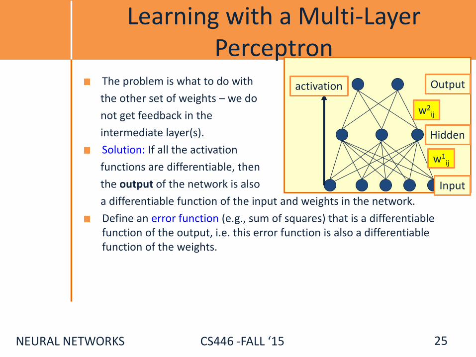
The problem is what to do with
the other set of weights – we do
not get feedback in the
intermediate layer(s).
Solution: If all the activation
functions are differentiable, then
the output of the network is also
a differentiable function of the input and weights in the network.
Define an error function (e.g., sum of squares) that is a differentiable function of the output, i.e. this error function is also a differentiable function of the weights.
25
activation
Input
Hidden
Output
w2ij
w1ij

NEURAL NETWORKS CS446 -FALL ‘15
Learning with a Multi-Layer Perceptron
The problem is what to do with
the other set of weights – we do
not get feedback in the
intermediate layer(s).
Solution: If all the activation
functions are differentiable, then
the output of the network is also
a differentiable function of the input and weights in the network.
Define an error function (e.g., sum of squares) that is a differentiable function of the output, i.e. this error function is also a differentiable function of the weights.
We can then evaluate the derivatives of the error with respect to the weights, and use these derivatives to find weight values that minimize this error function. This can be done, for example, using gradient descent (or other optimization methods).
This results in an algorithm called back-propagation.
25
activation
Input
Hidden
Output
w2ij
w1ij

NEURAL NETWORKS CS446 -FALL ‘15
Backpropagation Learning Rule
Since there could be multiple output units, we define the error as the sum over all the network output units.
𝐸𝑟𝑟 𝑤 =1
2∑ ∑𝑘∈𝐾 𝑡𝑘𝑑 − 𝑜𝑘𝑑
2𝑑∈𝐷
where 𝐷 is the set of training examples,
𝐾 is the set of output units
This can be used to derive the (global) learning rule which performs gradient descent in the weight space in an attempt to minimize the error function.
Δ𝑤𝑖𝑗 = −𝑅𝜕𝐸
𝜕𝑤𝑖𝑗
26
𝑜1…𝑜𝑘
(1, 0, 1, 0, 0)

NEURAL NETWORKS CS446 -FALL ‘15
Reminder: Model Neuron (Logistic)
Neuron is modeled by a unit 𝑗 connected by weighted links 𝑤𝑖𝑗 to other units 𝑖.
Use a non-linear, differentiable output function such as the
sigmoid or logistic function
Net input to a unit is defined as:
Output of a unit is defined as:
27
net𝑗 = ∑𝑤𝑖𝑗 . 𝑥𝑖
𝑜𝑗 =1
1 + exp −(net𝑗 − 𝑇𝑗)
𝑜𝑗
𝑥1 𝑥2 𝑥3 𝑥4 𝑥5 𝑥6
𝑥7 𝑤17
𝑤67

NEURAL NETWORKS CS446 -FALL ‘15
Derivation of Learning Rule
The weights are updated incrementally; the error is computed for each example and the weight update is then derived.
𝐸𝑟𝑟𝑑 𝑤 =1
2∑ 𝑡𝑘 − 𝑜𝑘
2𝑘∈𝐾
influences the output only through net𝑗
net𝑗 = ∑𝑤𝑖𝑗 . 𝑥𝑖𝑗
Therefore: 𝜕𝐸𝑑𝜕𝑤𝑖𝑗=𝜕𝐸𝑑𝜕net𝑗
𝜕net𝑗𝜕𝑤𝑖𝑗
28
𝑜1…𝑜𝑘
𝑗
𝑖
𝑤𝑖𝑗

NEURAL NETWORKS CS446 -FALL ‘15
Derivation of Learning Rule
et net 𝑗 𝑗𝑗 net 𝑗 =∑ 𝑤 𝑖𝑗 𝑤𝑤 𝑤 𝑖𝑗 𝑖𝑖𝑗𝑗 𝑤 𝑖𝑗 . 𝑥 𝑖𝑗 𝑥𝑥 𝑥 𝑖𝑗 𝑖𝑖𝑗𝑗 𝑥 𝑖𝑗
influences the output only through net 𝑗 net net 𝑗 𝑗𝑗 net 𝑗
The weights are updated incrementally; the error is computed for each example and the weight update is then derived.
𝐸𝑟𝑟𝑑 𝑤 =1
2∑ 𝑡𝑘 − 𝑜𝑘
2𝑘∈𝐾
𝑛et 𝑗 = ∑𝑤𝑖𝑗 . 𝑥𝑖𝑗
net𝑗 = ∑𝑤𝑖𝑗 . 𝑥𝑖𝑗
Therefore: 𝜕𝐸𝑑𝜕𝑤𝑖𝑗=𝜕𝐸𝑑𝜕net𝑗
𝜕net𝑗𝜕𝑤𝑖𝑗
28
𝑜1…𝑜𝑘
𝑗
𝑖
𝑤𝑖𝑗

NEURAL NETWORKS CS446 -FALL ‘15
Derivation of Learning Rule
𝜕 𝐸 𝑑 𝜕 net 𝑗 𝜕𝜕 𝐸 𝑑 𝐸𝐸 𝐸 𝑑 𝑑𝑑 𝐸 𝑑 𝜕 𝐸 𝑑 𝜕 net 𝑗 𝜕𝜕 net 𝑗 net net 𝑗 𝑗𝑗 net 𝑗 𝜕 𝐸 𝑑 𝜕 net 𝑗 𝜕 net 𝑗 𝜕 𝑤 𝑖𝑗 𝜕𝜕 net 𝑗 net net 𝑗 𝑗𝑗 net 𝑗 𝜕 net 𝑗 𝜕 𝑤 𝑖𝑗 𝜕𝜕 𝑤 𝑖𝑗 𝑤𝑤 𝑤 𝑖𝑗 𝑖𝑖𝑗𝑗 𝑤 𝑖𝑗 𝜕 net 𝑗 𝜕 𝑤 𝑖𝑗
et net 𝑗 𝑗𝑗 net 𝑗 =∑ 𝑤 𝑖𝑗 𝑤𝑤 𝑤 𝑖𝑗 𝑖𝑖𝑗𝑗 𝑤 𝑖𝑗 . 𝑥 𝑖𝑗 𝑥𝑥 𝑥 𝑖𝑗 𝑖𝑖𝑗𝑗 𝑥 𝑖𝑗
influences the output only through net 𝑗 net net 𝑗 𝑗𝑗 net 𝑗
The weights are updated incrementally; the error is computed for each example and the weight update is then derived.
𝐸𝑟𝑟𝑑 𝑤 =1
2∑ 𝑡𝑘 − 𝑜𝑘
2𝑘∈𝐾
Therefore: 𝜕 𝐸 𝑑 𝜕 𝑤 𝑖𝑗 = 𝐸 𝑑 𝜕 𝑤 𝑖𝑗 𝑖𝑗 𝑗 𝑖𝑗 𝐸 𝑑 𝜕 𝑤 𝑖𝑗 𝑑 𝑑 𝑑 𝐸 𝑑 𝜕 𝑤 𝑖𝑗
=𝜕𝐸𝑑𝜕net𝑗
𝜕net𝑗𝜕𝑤𝑖𝑗
Therefore: 𝜕𝐸𝑑𝜕𝑤𝑖𝑗=𝜕𝐸𝑑𝜕net𝑗
𝜕net𝑗𝜕𝑤𝑖𝑗
28
𝑜1…𝑜𝑘
𝑗
𝑖
𝑤𝑖𝑗

NEURAL NETWORKS CS446 -FALL ‘15
Derivation of Learning Rule (2)
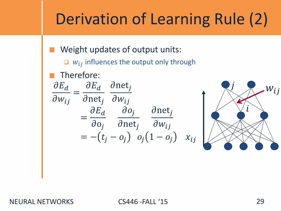
Weight updates of output units:
𝑤𝑖𝑗 influences the output only through
Therefore:
29
𝑗
𝑖
𝑤𝑖𝑗 𝜕𝐸𝑑𝜕𝑤𝑖𝑗=𝜕𝐸𝑑𝜕net𝑗 𝜕net𝑗𝜕𝑤𝑖𝑗

NEURAL NETWORKS CS446 -FALL ‘15
=𝜕𝐸𝑑𝜕o𝑗 𝜕𝑜𝑗
𝜕net𝑗 𝜕net𝑗
𝜕𝑤𝑖𝑗
Derivation of Learning Rule (2)
Weight updates of output units:
𝑤𝑖𝑗 influences the output only through
Therefore:
29
𝑗
𝑖
𝑤𝑖𝑗 𝜕𝐸𝑑𝜕𝑤𝑖𝑗=𝜕𝐸𝑑𝜕net𝑗 𝜕net𝑗𝜕𝑤𝑖𝑗
NEURAL NETWORKS CS446 -FALL ‘15
= − 𝑡𝑗 − 𝑜𝑗 𝑜𝑗 1 − 𝑜𝑗 𝑥𝑖𝑗
=𝜕𝐸𝑑𝜕o𝑗 𝜕𝑜𝑗
𝜕net𝑗 𝜕net𝑗
𝜕𝑤𝑖𝑗
Derivation of Learning Rule (2)
Weight updates of output units:
𝑤𝑖𝑗 influences the output only through
Therefore:
29
𝑗
𝑖
𝑤𝑖𝑗 𝜕𝐸𝑑𝜕𝑤𝑖𝑗=𝜕𝐸𝑑𝜕net𝑗 𝜕net𝑗𝜕𝑤𝑖𝑗

NEURAL NETWORKS CS446 -FALL ‘15
= − 𝑡𝑗 − 𝑜𝑗 𝑜𝑗 1 − 𝑜𝑗 𝑥𝑖𝑗
=𝜕𝐸𝑑𝜕o𝑗 𝜕𝑜𝑗
𝜕net𝑗 𝜕net𝑗
𝜕𝑤𝑖𝑗
Derivation of Learning Rule (2)
Weight updates of output units:
𝑤𝑖𝑗 influences the output only through
Therefore:
29
𝑗
𝑖
𝑤𝑖𝑗 𝜕𝐸𝑑𝜕𝑤𝑖𝑗=𝜕𝐸𝑑𝜕net𝑗 𝜕net𝑗𝜕𝑤𝑖𝑗

NEURAL NETWORKS CS446 -FALL ‘15
= − 𝑡𝑗 − 𝑜𝑗 𝑜𝑗 1 − 𝑜𝑗 𝑥𝑖𝑗
=𝜕𝐸𝑑𝜕o𝑗 𝜕𝑜𝑗
𝜕net𝑗 𝜕net𝑗
𝜕𝑤𝑖𝑗
Derivation of Learning Rule (2)
Weight updates of output units:
𝑤𝑖𝑗 influences the output only through
Therefore:
29
𝑗
𝑖
𝑤𝑖𝑗 𝜕𝐸𝑑𝜕𝑤𝑖𝑗=𝜕𝐸𝑑𝜕net𝑗 𝜕net𝑗𝜕𝑤𝑖𝑗
𝐸𝑟𝑟𝑑 𝑤 =1
2 𝑡𝑘 − 𝑜𝑘
2
𝑘∈𝐾

NEURAL NETWORKS CS446 -FALL ‘15
= − 𝑡𝑗 − 𝑜𝑗 𝑜𝑗 1 − 𝑜𝑗 𝑥𝑖𝑗
=𝜕𝐸𝑑𝜕o𝑗 𝜕𝑜𝑗
𝜕net𝑗 𝜕net𝑗
𝜕𝑤𝑖𝑗
Derivation of Learning Rule (2)
Weight updates of output units:
𝑤𝑖𝑗 influences the output only through
Therefore:
29
𝑗
𝑖
𝑤𝑖𝑗 𝜕𝐸𝑑𝜕𝑤𝑖𝑗=𝜕𝐸𝑑𝜕net𝑗 𝜕net𝑗𝜕𝑤𝑖𝑗

NEURAL NETWORKS CS446 -FALL ‘15
= − 𝑡𝑗 − 𝑜𝑗 𝑜𝑗 1 − 𝑜𝑗 𝑥𝑖𝑗
=𝜕𝐸𝑑𝜕o𝑗 𝜕𝑜𝑗
𝜕net𝑗 𝜕net𝑗
𝜕𝑤𝑖𝑗
Derivation of Learning Rule (2)
Weight updates of output units:
𝑤𝑖𝑗 influences the output only through
Therefore:
29
𝑗
𝑖
𝑤𝑖𝑗 𝜕𝐸𝑑𝜕𝑤𝑖𝑗=𝜕𝐸𝑑𝜕net𝑗 𝜕net𝑗𝜕𝑤𝑖𝑗

NEURAL NETWORKS CS446 -FALL ‘15
= − 𝑡𝑗 − 𝑜𝑗 𝑜𝑗 1 − 𝑜𝑗 𝑥𝑖𝑗
=𝜕𝐸𝑑𝜕o𝑗 𝜕𝑜𝑗
𝜕net𝑗 𝜕net𝑗
𝜕𝑤𝑖𝑗
Derivation of Learning Rule (2)
Weight updates of output units:
𝑤𝑖𝑗 influences the output only through
Therefore:
29
𝑗
𝑖
𝑤𝑖𝑗 𝜕𝐸𝑑𝜕𝑤𝑖𝑗=𝜕𝐸𝑑𝜕net𝑗 𝜕net𝑗𝜕𝑤𝑖𝑗
𝜕𝑜𝑗
𝜕net𝑗= 𝑜𝑗(1 − 𝑜𝑗)
𝑜𝑗 =1
1 + exp{−(net𝑗 − 𝑇𝑗)}

NEURAL NETWORKS CS446 -FALL ‘15
= − 𝑡𝑗 − 𝑜𝑗 𝑜𝑗 1 − 𝑜𝑗 𝑥𝑖𝑗
=𝜕𝐸𝑑𝜕o𝑗 𝜕𝑜𝑗
𝜕net𝑗 𝜕net𝑗
𝜕𝑤𝑖𝑗
Derivation of Learning Rule (2)
Weight updates of output units:
𝑤𝑖𝑗 influences the output only through
Therefore:
29
𝑗
𝑖
𝑤𝑖𝑗 𝜕𝐸𝑑𝜕𝑤𝑖𝑗=𝜕𝐸𝑑𝜕net𝑗 𝜕net𝑗𝜕𝑤𝑖𝑗

NEURAL NETWORKS CS446 -FALL ‘15
= − 𝑡𝑗 − 𝑜𝑗 𝑜𝑗 1 − 𝑜𝑗 𝑥𝑖𝑗
=𝜕𝐸𝑑𝜕o𝑗 𝜕𝑜𝑗
𝜕net𝑗 𝜕net𝑗
𝜕𝑤𝑖𝑗
Derivation of Learning Rule (2)
Weight updates of output units:
𝑤𝑖𝑗 influences the output only through
Therefore:
29
𝑗
𝑖
𝑤𝑖𝑗 𝜕𝐸𝑑𝜕𝑤𝑖𝑗=𝜕𝐸𝑑𝜕net𝑗 𝜕net𝑗𝜕𝑤𝑖𝑗

NEURAL NETWORKS CS446 -FALL ‘15
= − 𝑡𝑗 − 𝑜𝑗 𝑜𝑗 1 − 𝑜𝑗 𝑥𝑖𝑗
=𝜕𝐸𝑑𝜕o𝑗 𝜕𝑜𝑗
𝜕net𝑗 𝜕net𝑗
𝜕𝑤𝑖𝑗
Derivation of Learning Rule (2)
Weight updates of output units:
𝑤𝑖𝑗 influences the output only through
Therefore:
29
𝑗
𝑖
𝑤𝑖𝑗 𝜕𝐸𝑑𝜕𝑤𝑖𝑗=𝜕𝐸𝑑𝜕net𝑗 𝜕net𝑗𝜕𝑤𝑖𝑗
net𝑗 = ∑𝑤𝑖𝑗 . 𝑥𝑖𝑗

NEURAL NETWORKS CS446 -FALL ‘15
Derivation of Learning Rule (3)
Weights of output units:
𝑤𝑖𝑗 is changed by:
where
𝛿𝑗 = 𝑡𝑗 − 𝑜𝑗 𝑜𝑗 1 − 𝑜𝑗
30
Δ𝑤𝑖𝑗 = 𝑅 𝑡𝑗 − 𝑜𝑗 𝑜𝑗 1 − 𝑜𝑗 𝑥𝑖𝑗= 𝑅𝛿𝑗𝑥𝑖𝑗
𝑗
𝑖
𝑤𝑖𝑗
𝑜𝑗
𝑥𝑖𝑗

NEURAL NETWORKS CS446 -FALL ‘15
𝜕𝐸𝑑𝜕𝑤𝑖𝑗=𝜕𝐸𝑑𝜕net𝑗 𝜕net𝑗𝜕𝑤𝑖𝑗=
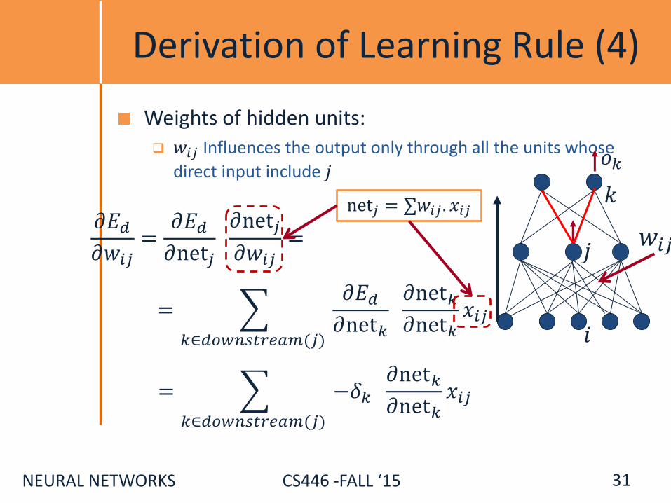
Derivation of Learning Rule (4)
Weights of hidden units:
𝑤𝑖𝑗 Influences the output only through all the units whose
direct input include 𝑗
31
𝑘 𝑗
𝑖
𝑤𝑖𝑗
𝑜𝑘

NEURAL NETWORKS CS446 -FALL ‘15
= 𝜕𝐸𝑑𝜕net𝑘 𝜕net𝑘𝜕net𝑘
𝑥𝑖𝑗𝑘∈𝑑𝑜𝑤𝑛𝑠𝑡𝑟𝑒𝑎𝑚(𝑗)
𝜕𝐸𝑑𝜕𝑤𝑖𝑗=𝜕𝐸𝑑𝜕net𝑗 𝜕net𝑗𝜕𝑤𝑖𝑗=
Derivation of Learning Rule (4)
Weights of hidden units:
𝑤𝑖𝑗 Influences the output only through all the units whose
direct input include 𝑗
31
𝑘 𝑗
𝑖
𝑤𝑖𝑗
𝑜𝑘

NEURAL NETWORKS CS446 -FALL ‘15
= 𝜕𝐸𝑑𝜕net𝑘 𝜕net𝑘𝜕net𝑘
𝑥𝑖𝑗𝑘∈𝑑𝑜𝑤𝑛𝑠𝑡𝑟𝑒𝑎𝑚(𝑗)
𝜕𝐸𝑑𝜕𝑤𝑖𝑗=𝜕𝐸𝑑𝜕net𝑗 𝜕net𝑗𝜕𝑤𝑖𝑗=
Derivation of Learning Rule (4)
Weights of hidden units:
𝑤𝑖𝑗 Influences the output only through all the units whose
direct input include 𝑗
31
𝑘 𝑗
𝑖
𝑤𝑖𝑗
𝑜𝑘
net𝑗 = ∑𝑤𝑖𝑗 . 𝑥𝑖𝑗
NEURAL NETWORKS CS446 -FALL ‘15
= −𝛿𝑘 𝜕net𝑘𝜕net𝑘
𝑥𝑖𝑗𝑘∈𝑑𝑜𝑤𝑛𝑠𝑡𝑟𝑒𝑎𝑚(𝑗)
= 𝜕𝐸𝑑𝜕net𝑘 𝜕net𝑘𝜕net𝑘
𝑥𝑖𝑗𝑘∈𝑑𝑜𝑤𝑛𝑠𝑡𝑟𝑒𝑎𝑚(𝑗)
𝜕𝐸𝑑𝜕𝑤𝑖𝑗=𝜕𝐸𝑑𝜕net𝑗 𝜕net𝑗𝜕𝑤𝑖𝑗=
Derivation of Learning Rule (4)
Weights of hidden units:
𝑤𝑖𝑗 Influences the output only through all the units whose
direct input include 𝑗
31
𝑘 𝑗
𝑖
𝑤𝑖𝑗
𝑜𝑘
net𝑗 = ∑𝑤𝑖𝑗 . 𝑥𝑖𝑗

NEURAL NETWORKS CS446 -FALL ‘15
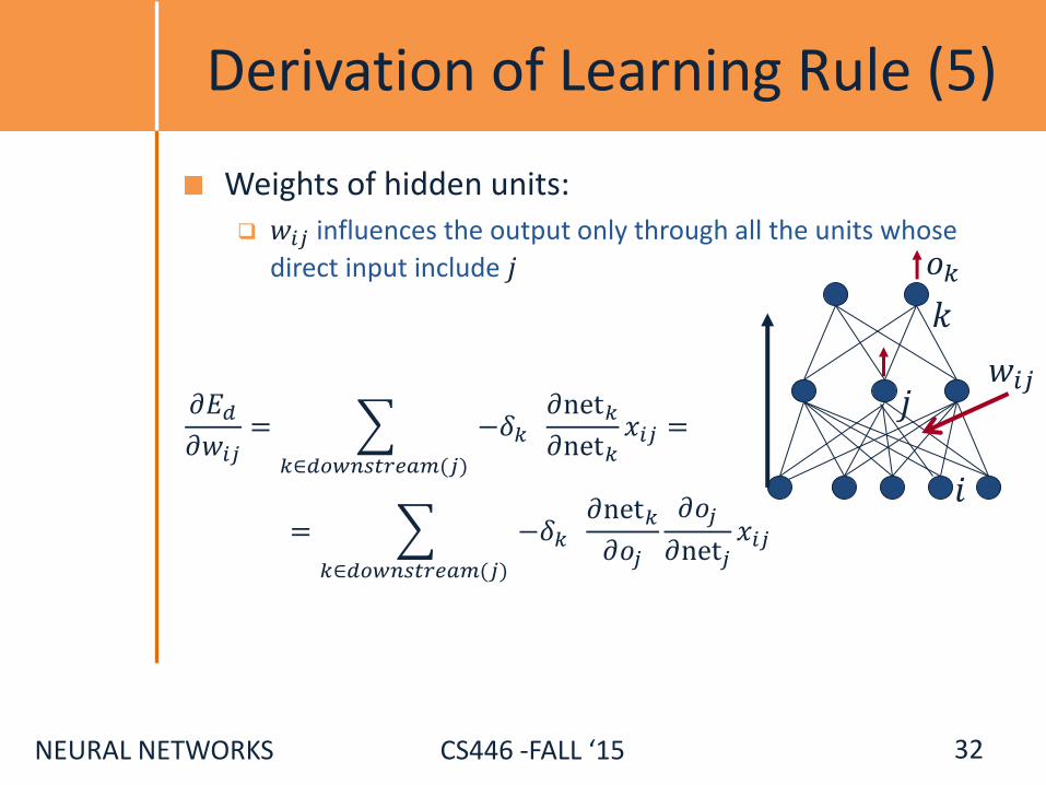
Derivation of Learning Rule (5)
Weights of hidden units:
𝑤𝑖𝑗 influences the output only through all the units whose
direct input include 𝑗
32
𝑘 𝑗
𝑖
𝑤𝑖𝑗
𝑜𝑘
𝜕𝐸𝑑𝜕𝑤𝑖𝑗= −𝛿𝑘
𝜕net𝑘𝜕net𝑘
𝑥𝑖𝑗𝑘∈𝑑𝑜𝑤𝑛𝑠𝑡𝑟𝑒𝑎𝑚(𝑗)
=
NEURAL NETWORKS CS446 -FALL ‘15
= −𝛿𝑘 𝜕net𝑘𝜕𝑜𝑗
𝜕𝑜𝑗
𝜕net𝑗𝑥𝑖𝑗
𝑘∈𝑑𝑜𝑤𝑛𝑠𝑡𝑟𝑒𝑎𝑚(𝑗)
Derivation of Learning Rule (5)
Weights of hidden units:
𝑤𝑖𝑗 influences the output only through all the units whose
direct input include 𝑗
32
𝑘 𝑗
𝑖
𝑤𝑖𝑗
𝑜𝑘
𝜕𝐸𝑑𝜕𝑤𝑖𝑗= −𝛿𝑘
𝜕net𝑘𝜕net𝑘
𝑥𝑖𝑗𝑘∈𝑑𝑜𝑤𝑛𝑠𝑡𝑟𝑒𝑎𝑚(𝑗)
=

NEURAL NETWORKS CS446 -FALL ‘15
= −𝛿𝑘 𝜕net𝑘𝜕𝑜𝑗
𝜕𝑜𝑗
𝜕net𝑗𝑥𝑖𝑗
𝑘∈𝑑𝑜𝑤𝑛𝑠𝑡𝑟𝑒𝑎𝑚(𝑗)
= −𝛿𝑘 𝑤𝑗𝑘 𝑜𝑗(1 − 𝑜𝑗) 𝑥𝑖𝑗𝑘∈𝑑𝑜𝑤𝑛𝑠𝑡𝑟𝑒𝑎𝑚(𝑗)
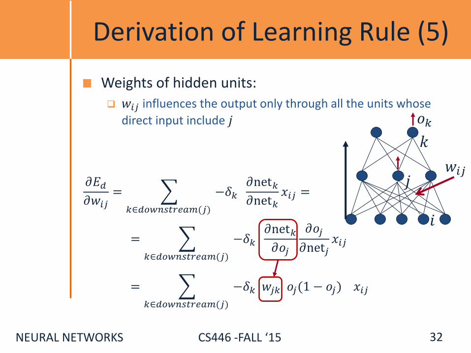
Derivation of Learning Rule (5)
Weights of hidden units:
𝑤𝑖𝑗 influences the output only through all the units whose
direct input include 𝑗
32
𝑘 𝑗
𝑖
𝑤𝑖𝑗
𝑜𝑘
𝜕𝐸𝑑𝜕𝑤𝑖𝑗= −𝛿𝑘
𝜕net𝑘𝜕net𝑘
𝑥𝑖𝑗𝑘∈𝑑𝑜𝑤𝑛𝑠𝑡𝑟𝑒𝑎𝑚(𝑗)
=
NEURAL NETWORKS CS446 -FALL ‘15
= −𝛿𝑘 𝜕net𝑘𝜕𝑜𝑗
𝜕𝑜𝑗
𝜕net𝑗𝑥𝑖𝑗
𝑘∈𝑑𝑜𝑤𝑛𝑠𝑡𝑟𝑒𝑎𝑚(𝑗)
= −𝛿𝑘 𝑤𝑗𝑘 𝑜𝑗(1 − 𝑜𝑗) 𝑥𝑖𝑗𝑘∈𝑑𝑜𝑤𝑛𝑠𝑡𝑟𝑒𝑎𝑚(𝑗)
Derivation of Learning Rule (5)
Weights of hidden units:
𝑤𝑖𝑗 influences the output only through all the units whose
direct input include 𝑗
32
𝑘 𝑗
𝑖
𝑤𝑖𝑗
𝑜𝑘
𝜕𝐸𝑑𝜕𝑤𝑖𝑗= −𝛿𝑘
𝜕net𝑘𝜕net𝑘
𝑥𝑖𝑗𝑘∈𝑑𝑜𝑤𝑛𝑠𝑡𝑟𝑒𝑎𝑚(𝑗)
=

NEURAL NETWORKS CS446 -FALL ‘15
Derivation of Learning Rule (6)
Weights of hidden units:
𝑤𝑖𝑗 is changed by:
Where
𝛿𝑗 = 𝑜𝑗 1 − 𝑜𝑗 . −𝛿𝑘 𝑤𝑗𝑘
𝑘∈𝑑𝑜𝑤𝑛𝑠𝑡𝑟𝑒𝑎𝑚 𝑗
First determine the error for the output units.
Then, backpropagate this error layer by layer through the network, changing weights appropriately in each layer.
33
𝑘 𝑗
𝑖
𝑤𝑖𝑗
𝑜𝑘
Δ𝑤𝑖𝑗 = 𝑅 𝑜𝑗 1 − 𝑜𝑗 . −𝛿𝑘 𝑤𝑗𝑘
𝑘∈𝑑𝑜𝑤𝑛𝑠𝑡𝑟𝑒𝑎𝑚 𝑗
𝑥𝑖𝑗
= 𝑅𝛿𝑗𝑥𝑖𝑗

NEURAL NETWORKS CS446 -FALL ‘15
The Backpropagation Algorithm
Create a fully connected three layer network. Initialize weights.
Until all examples produce the correct output within 𝜖 (or other criteria)
For each example in the training set do:
1. Compute the network output for this example
2. Compute the error between the output and target value 𝛿𝑘 = 𝑡𝑘 − 𝑜𝑘 𝑜𝑘 1 − 𝑜𝑘
1. For each output unit k, compute error term
𝛿𝑗 = 𝑜𝑗 1 − 𝑜𝑗 . −𝛿𝑘 𝑤𝑗𝑘
𝑘∈𝑑𝑜𝑤𝑛𝑠𝑡𝑟𝑒𝑎𝑚 𝑗
1. For each hidden unit, compute error term: Δ𝑤𝑖𝑗 = 𝑅𝛿𝑗𝑥𝑖𝑗
1. Update network weights
End epoch
34

NEURAL NETWORKS CS446 -FALL ‘15
More Hidden Layers
The same algorithm holds for more hidden layers.
35
input ℎ1 ℎ2 ℎ3 output

NEURAL NETWORKS CS446 -FALL ‘15
Comments on Training
No guarantee of convergence; may oscillate or reach a local minima.
In practice, many large networks can be trained on large amounts of data for realistic problems.
36

NEURAL NETWORKS CS446 -FALL ‘15
Comments on Training
No guarantee of convergence; may oscillate or reach a local minima.
In practice, many large networks can be trained on large amounts of data for realistic problems.
Many epochs (tens of thousands) may be needed for adequate training. Large data sets may require many hours of CPU
Termination criteria: Number of epochs; Threshold on training set error; No decrease in error; Increased error on a validation set.
To avoid local minima: several trials with different random initial weights with majority or voting techniques
36

NEURAL NETWORKS CS446 -FALL ‘15
Over-training Prevention
Running too many epochs may over-train the network and result in over-fitting. (improved result on training, decrease in performance on test set)
37

NEURAL NETWORKS CS446 -FALL ‘15
Over-training Prevention
Running too many epochs may over-train the network and result in over-fitting. (improved result on training, decrease in performance on test set)
Keep an hold-out validation set and test accuracy after every epoch
Maintain weights for best performing network on the validation set and return it when performance decreases significantly beyond that.
To avoid losing training data to validation: Use 10-fold cross-validation to determine the average number of
epochs that optimizes validation performance
Train on the full data set using this many epochs to produce the final results
37

NEURAL NETWORKS CS446 -FALL ‘15
Over-fitting prevention
Too few hidden units prevent the system from adequately fitting the data and learning the concept.
Using too many hidden units leads to over-fitting.
Similar cross-validation method can be used to determine an appropriate number of hidden units. (general)
Another approach to prevent over-fitting is weight-decay: all weights are multiplied by some fraction in (0,1) after every epoch. Encourages smaller weights and less complex hypothesis
Equivalently: change Error function to include a term for the sum of the squares of the weights in the network. (general)
38
NEURAL NETWORKS CS446 -FALL ‘15
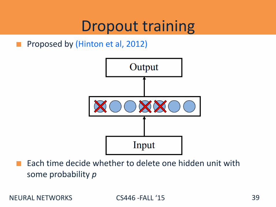
Dropout training Proposed by (Hinton et al, 2012)
Each time decide whether to delete one hidden unit with some probability p
39
NEURAL NETWORKS CS446 -FALL ‘15
Dropout training
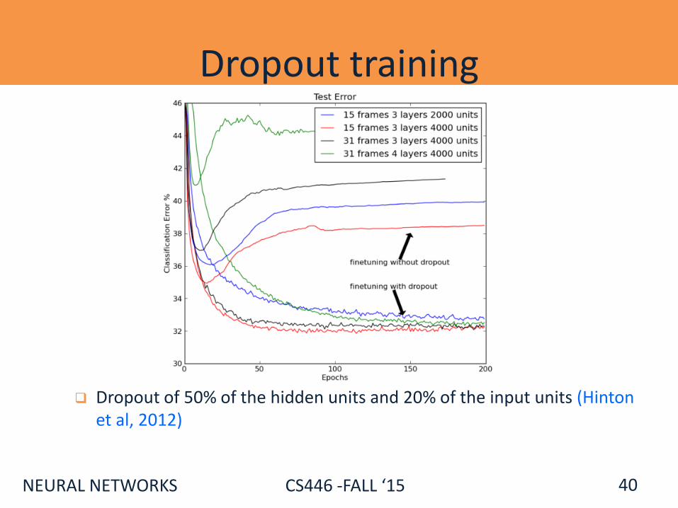
Dropout of 50% of the hidden units and 20% of the input units (Hinton et al, 2012)
40
NEURAL NETWORKS CS446 -FALL ‘15
Dropout training Model averaging effect
Among models, with shared parameters
H: number of units in the network
Only a few get trained
Much stronger than the known regularizer
2H
41

NEURAL NETWORKS CS446 -FALL ‘15
Dropout training Model averaging effect
Among models, with shared parameters
H: number of units in the network
Only a few get trained
Much stronger than the known regularizer
What about the input space?
Do the same thing!
2H
41

NEURAL NETWORKS CS446 -FALL ‘15
Input-Output Coding
Appropriate coding of inputs and outputs can make learning problem easier and improve generalization.
Encode each binary feature as a separate input unit;
For multi-valued features include one binary unit per value rather than trying to encode input information in fewer units.
For disjoint categorization problem, best to have one output unit for each category rather than encoding N categories into log N bits.
42

NEURAL NETWORKS CS446 -FALL ‘15
Representational Power
The Backpropagation version presented is for networks with a single hidden layer,
But:
Any Boolean function can be represented by a two layer network (simulate a two layer AND-OR network)
Any bounded continuous function can be approximated with arbitrary small error by a two layer network.
Sigmoid functions provide a set of basis function from which arbitrary function can be composed.
Any function can be approximated to arbitrary accuracy by a three layer network.
43
NEURAL NETWORKS CS446 -FALL ‘15
Hidden Layer Representation
Weight tuning procedure sets weights that define whatever hidden units representation is most effective at minimizing the error.
Sometimes Backpropagation will define new hidden layer features that are not explicit in the input representation, but which capture properties of the input instances that are most relevant to learning the target function.
Trained hidden units can be seen as newly constructed features that re-represent the examples so that they are linearly separable
44

NEURAL NETWORKS CS446 -FALL ‘15
Auto-associative Network
An auto-associative network trained with 8 inputs, 3 hidden units and 8 output nodes, where the output must reproduce the input.
When trained with vectors with only one bit on
INPUT HIDDEN
1 0 0 0 0 0 0 0 .89 .40 0.8
0 1 0 0 0 0 0 0 .97 .99 .71
….
0 0 0 0 0 0 0 1 .01 .11 .88
Learned the standard 3-bit encoding for the 8 bit vectors.
Illustrates also data compression aspects of learning
45
1 0 0 0 1 0 0 0
1 0 0 0 1 0 0 0