No Asymmetry in Pay for Luck

Naveen D. Daniela

Yuanzhi Lib Lalitha Naveenc

October 2012

Abstract

______________________________________________________________________________

In contrast with current literature, we find no asymmetry in CEO pay for luck. The current literature documents that CEOs are rewarded for performance increases due to good luck but are not penalized to the same extent for performance decreases due to bad luck. These studies are based on either the level of annual pay or the change in annual pay. These measures, however, constitute only a trivial fraction of CEO compensation linked to firm performance (Aggarwal and Samwick (1999)). CEOs are affected by changes in their total firm-related wealth, which in turn is affected to a greater extent by equity holdings rather than annual pay (Jensen and Murphy (1990) and Core and Guay (2002)). We find that, on average, the CEO’s firm-related wealth increases by $37 for a $1000 increase in shareholder wealth due to good luck, which is identical to the decrease of $37 for a $1000 decrease in shareholder wealth due to bad luck.

_____________________________________________________________________________________

JEL Classifications: G32; G34 Keywords: Asymmetry in pay for luck, Pay for luck, Pay-performance-sensitivity, Compensation, Firm-related wealth ______________________________________________________________________________ a LeBow College of Business, Drexel University, Philadelphia, PA, 19104, USA; nav@drexel.edu b Fox School of Business, Temple University, Philadelphia, PA, 19122, USA; yuanzhi.li@temple.edu c Fox School of Business, Temple University, Philadelphia, PA, 19122, USA; lnaveen@temple.edu The authors are grateful for helpful comments from Rajesh Aggarwal, Jay Cai, Eli Fich, Gerald Garvey, Radhakrishnan Gopalan, Swaminathan Kalpathy, Xi Li, Connie Mao, Todd Milbourn, Oleg Rytchkov, Fenghua Song, Ralph Walkling, David Yermack, and seminar participants at Drexel University, Temple University, and Villanova University.

1

No Asymmetry in Pay for Luck

Recent studies (Garvey and Milbourn (2006) and Gopalan, Milbourn, and Song (2010))

document an asymmetry in CEO pay for luck. Specifically, these studies show that CEOs are

rewarded for firm performance that is attributed to good luck, but not penalized to the same

extent for performance that is attributed to bad luck. The findings of Garvey and Milbourn

(2006) have been interpreted by several studies as being consistent with the rent extraction view

of compensation contracts.1 Using an improved research design that is grounded in prior

literature, we find no asymmetry in pay for luck.

Previous studies that examine asymmetry in CEO pay for luck estimate regressions where

the dependent variable is change in annual pay (Garvey and Milbourn (2006)) or the level of

annual pay (Gopalan, Milbourn, and Song (2010)), and the independent variables are measures

of dollar stock returns attributable to good luck and bad luck.2 In contrast, our dependent

variable is the annual change in the CEO’s firm-related wealth, which includes the annual pay

but also the value change from the CEO’s stock and option holdings. The change in firm-related

wealth is affected to a greater extent by equity holdings rather than annual pay. In fact,

Aggarwal and Samwick (1999) find that the pay-performance-sensitivity estimated using the

change in the CEO’s firm-related wealth is about 20 times higher than that estimated using the

change in annual pay and 33 times higher than that estimated using the level of annual pay.3

Thus, Garvey and Milbourn (2006) and Gopalan, Milbourn, and Song (2010), by focusing on

1 For example, Frydman and Jenter (2010, pg. 16), in their survey of the compensation literature, state “Rent‐extraction is also suggested by the observation that CEOs are frequently rewarded for lucky events that are not under their control (such as an improving economy) but not equally penalized for unlucky events (Bertrand & Mullainathan 2001, Garvey & Milbourn 2006).” 2 Gopalan et al. use the term “pay for sector performance” rather than “pay for luck.” 3 The numbers are based on the pay-performance-sensitivity for the median-risk firm reported in Model 1, Panel A of Table 3 (pay-performance-sensitivity = 14.523), Model 1, Panel A of Table 4 (pay-performance-sensitivity = 0.732)), and Model 2, Panel A of Table 4 (pay-performance-sensitivity = 0.432) of their paper.

2

annual pay, are effectively examining only a small slice of the overall pay-for-performance

sensitivity. The conclusions from such studies, therefore, may be premature.

Two related strands of the literature provide strong support for our choice of change in

the CEO’s firm-related wealth as the dependent variable. First, early papers that examine ex-post

pay-for-performance––but without separating performance into skill and luck––use the annual

change in the CEO’s firm-related wealth (Jensen and Murphy (1990), Hall and Liebman (1998),

Aggarwal and Samwick (1999), and Milbourn (2003)). These studies use the term “pay-

performance-sensitivity” (PPS)––a misnomer in some sense––to represent the change in CEO

firm-related wealth associated with the change in shareholder wealth. Hall and Liebman (pg.

670) argue that “CEOs care about changes in their wealth emanating from all sources, not just

salary and bonus” and that changes in firm-related wealth that include changes in the value of

stocks and options “...is the right measure of monetary incentives.” The idea that change in

wealth is more important to managers is reinforced by the loss in firm-related wealth, suffered by

the CEOs of firms such as Bear Sterns and Lehman Brothers, resulting from the steep fall in their

share prices. As Yermack (2009b) notes, CEOs of financial firms received several million

dollars in salary and perks, but their wealth declined significantly in 2008 as their stock prices

nosedived. He argues that this indicates a robust pay-for-performance system. Fahlenbrach and

Stulz (2011) provide validation for Yermack’s arguments by showing that bank CEOs suffered

large wealth losses during the recent crisis.

Second, the ex-ante managerial incentives literature (Guay (1999) and Core and Guay

(1999, 2002)) considers incentives from the entire portfolio of stock and options, and not just

those from annual grants. Indeed, Core and Guay (2002) argue that “[f]ailure to capture all the

components of CEOs’ equity incentives results in measurement error that can either reduce the

3

power of the researcher's tests or lead to spurious inferences.”

We capitalize on improved data availability and refine the methodology used in earlier

studies (Jensen and Murphy (1990), Hall and Liebman (1998), and Aggarwal and Samwick

(1999)) to more precisely estimate the change in the CEO’s firm-related wealth. These studies

have estimated changes in firm-related wealth typically by multiplying the starting portfolio of

stock and options by their corresponding return during the year and then adding the annual pay

(which includes the value of equity grants). This method assumes that CEOs do not engage in

stock sales, stock purchases, or option exercises during the year, and also ignores option

repricing, options expiring out of the money, and any change in value of equity grants from the

grant date to the fiscal year end date. Our methodology addresses these limitations. Section II.A

and the Appendix provide more details of our measure of changes in firm-related wealth.

We use data from ExecuComp for the period 1992–2005 to be comparable with Gopalan,

Milbourn, and Song (2010) and to help us isolate the impact of changing the dependent variable

on pay-for-luck asymmetry.4 Our results are robust to extending the sample period to 2010.

We find that the average value of the stock and option portfolio ($61.90M) is many times

larger than the average annual pay ($3.83M). Thus it is reasonable to believe that wealth gain is

driven primarily by changes in value of the stock and option portfolio and not by the change in

annual pay or the level of annual pay. Consistent with this, we find that the average change in

firm-related wealth ($11.31M) is significantly larger than the average change in pay ($0.21M).

Our estimate of annual changes in the CEO’s firm-related wealth has a correlation of 0.16 with

the change in annual pay and a correlation of 0.23 with the level of annual pay. The low

4 Garvey and Milbourn include data from 1992-2001 while Gopalan et al. include data from 1992-2006. We do not include 2006 because this was the transition year when firms changed their compensation reporting significantly as part of FAS 123R requirements. In 2006, about 15% of firms still reported their data using the old reporting format. We wish to ensure that our results are not driven by changes in these reporting requirements. Our results are unaffected if we include 2006 in our sample.

4

correlations suggest that examining change in wealth need not lead to the same inferences as

examining change in pay or level of pay.

We start by replicating the key specifications in the papers that document pay-for-luck

asymmetry: Model 1, Table 5 of Garvey and Milbourn (2006, henceforth GM) and Panel A,

Table 9 of Gopalan, Milbourn, and Song (2010, henceforth GMS). Similar to these studies, we

find asymmetry in pay for luck. We then replicate the same regressions, but using our estimate

of annual change in the CEO’s firm-related wealth as the dependent variable. We now find no

asymmetry in pay for luck. We find that the CEO’s firm-related wealth increases by $37.210 for

a $1000 increase in shareholder wealth due to good luck, which is economically and statistically

indistinguishable from the decrease of $37.208 for a $1000 decrease in shareholder wealth due to

bad luck. Our evidence does not support the skimming view prevalent in the literature.

GM and GMS document pay-for-luck asymmetry in specific subsamples of firms such as

those with weak shareholder rights, diversified firms, firms with greater strategic flexibility, and

firms with talented CEOs. In contrast to both studies, we find no asymmetry in pay for luck in

similar subsamples when we use change in firm-related wealth as the dependent variable.

Our results are intuitive: the CEO’s firm-related wealth comprises primarily of stock and

option holdings, the value of which moves with the stock price. The stock price, in turn,

responds in the same manner to both good and bad luck, leading to our finding of no asymmetry.

So what explains the GM and GMS results? One possible explanation for the asymmetry in pay

for luck documented by GMS is that, in reality, there is a lower bound on annual pay (much

higher than zero), which is dictated by the reservation wage demanded by the CEO. Therefore

the board, when faced with poor firm performance, cannot reduce CEO pay as much as it would

like. This also explains the GM finding of asymmetry in pay for luck, because the change in

5

annual pay cannot be significantly negative despite poor performance.

We perform several robustness checks to confirm our result. First, we recognize that the

widely-used Core and Guay methodology, which we use to compute option values prior to 2006,

has some limitations. We rule out the possibility that this methodology biases our results by

documenting that our findings continue to hold for the period 2007–2010 (where this

methodology is not required). Second, we find no evidence of pay for luck asymmetry when we

use alternative measures of luck and skill, alternative definitions of change in wealth, alternative

non-linear functional forms, different proxies for CEO power, alternative measures of

governance, as well as alternative econometric specifications.

Third, we examine more closely the link between option compensation and asymmetry in

pay for luck. CEO compensation typically includes options, whose values have a convex

relation with stock price. Therefore, one might expect a non-linear relation in pay for

performance. Moreover, this asymmetry in pay for performance will be stronger if the options

are near the money and if the options have shorter time-to-maturity. This asymmetry in pay for

performance will not translate into an asymmetry in pay for luck, however, if (i) luck is not

highly correlated with overall performance or (ii) annual pay following poor performance is high

enough to compensate for the loss in value of equity holdings. While we find a modestly high

correlation between luck and performance (=0.53), it is likely that firms give higher equity

awards (and hence higher pay) following poor performance to bring the level of incentives closer

to target (Core and Guay (1999)). Thus, we do not expect to find a link between the structure of

option compensation and asymmetry in pay for luck. Consistent with this, we find no

asymmetry in pay for luck even in firms whose CEOs have a significant amount of options

(option value accounts for more than 80% of firm-related wealth), whose CEOs have option

6

portfolios with a short maturity, or whose CEOs have option portfolios that are near the money.

One potential concern here is that our specifications somehow lack the statistical power

necessary to reject the implied null of no asymmetry. We believe this is not a valid argument

because we are able to replicate the findings in GM and GMS when we use the same dependent

variables as in their study. We fail to find their result only when we use change in firm-related

wealth as the dependent variable. Moreover, using change in firm-related wealth, we are able to

replicate the results in Aggarwal and Samwick (1999). Thus it is unlikely to be a lack of

statistical power that is driving our results. Importantly, the results are never economically

significant. For our overall sample, change in wealth associated with good luck is almost

identical to the change in wealth associated with bad luck.

The main contribution of our study is to document that when an all-inclusive measure of

incentives––changes in the CEO’s firm-related wealth––is used, there is no asymmetry in pay for

luck. Our secondary contribution is methodological: we provide researchers with a methodology

to more precisely estimate the changes in the CEO’s firm-related wealth.

The rest of the paper is arranged as follows. Section I briefly reviews the related

literature and establishes the basis for our research design. Section II describes the data and

provides descriptive statistics. Section III presents our main results. Section IV presents several

robustness tests, and Section V concludes.

I. Motivation and Related Literature

One of the key predictions of agency theory is that compensation will be designed to

incentivize managers to maximize shareholder wealth. One such mechanism is the sensitivity of

managerial pay to firm performance. Jensen and Murphy (1990) was the first comprehensive

study on pay-performance incentives. The authors estimate that for every $1000 change in

7

shareholder wealth, the CEO’s firm-related wealth changes, on average, by $3.25, where change

in CEO firm-related wealth is calculated as the sum of changes in value of outstanding stock

options and stock holdings, annual pay, present value of future changes in salary and bonus, and

present value of loss in pay associated with performance-related dismissals.

Subsequently, Hall and Liebman (1998) document that the pay-performance sensitivities

are much higher than that estimated by Jensen and Murphy, primarily because of the increase in

stock option awards over their sample period. They estimate changes in wealth as the increase in

the value of the CEO’s beginning-of-year holdings of firm stock and options plus salary and

bonus plus value of stock and option grants. Aggarwal and Samwick (1999) document that

changes in firm-related wealth (calculated similar to Hall and Liebman) are positively associated

with firm performance, but this pay-performance sensitivity is a declining function of firm risk.

A related strand of literature on relative performance evaluation considers the sensitivity

of pay changes to the performance of the firm net of industry (or market) performance (Gibbons

and Murphy (1990), Himmelberg and Hubbard (2000), Garvey and Milbourn (2003), Rajgopal,

Shevlin, and Zamora (2006)). With the exception of Gibbons and Murphy, all these papers

consider changes in firm-related wealth. Bertrand and Mullainathan (2001), although they

belong to this broad stream of literature, use the term ‘luck’ to describe the performance of the

firm that can be attributed to external forces (such as oil prices for oil industry firms, or exchange

rate movements, or industry returns), and the term ‘skill’ to describe firm performance net of

luck. They find that CEO pay is as sensitive to luck as it is to changes in aggregate firm

performance, and the sensitivity of CEO pay to luck is higher in poorly governed firms. They

interpret this as evidence of managerial skimming. While the authors note (pg. 905) that

“[i]deally, the compensation in a given year would also include changes in the value of

8

unexercised options granted in previous years [Hall and Liebman, 1998]” they use change in pay

as the dependent variable because “calculation [of wealth changes] requires data on the

accumulated stock of options held by the CEO each year, whereas existing data sets including

ours, contain only information on new options granted each year.”

Garvey and Milbourn (2006, GM) contend that higher sensitivity of CEO pay to luck in

weakly governed firms is not sufficient to prove rent extraction; rather there should be

asymmetry in pay for luck. Specifically, they argue that CEOs would like to be rewarded for

good luck, but insulated somewhat from bad luck. Using change in annual CEO pay, they find

an asymmetry in CEO pay for luck. This asymmetry is stronger in weakly governed firms. They

interpret the overall findings as indicative of rent extraction.5

Following Bertrand and Mullainathan (2001), GM use change in annual pay rather than

changes in firm-related wealth. As mentioned earlier, however, Bertrand and Mullainathan note

that pay-for-luck tests should ideally be done using changes in the firm-related wealth of the

CEO, but are unable to do so due to data limitations. GM, however, do not suffer from the same

data limitations because they use ExecuComp data, which could be used to estimate changes in

firm-related wealth. They explain their use of change in pay (rather than change in firm-related

wealth) as follows: “we ignore changes in the value of CEO’s existing shares and options

because by definition they move only with the stock price and cannot have distinct sensitivities

to luck and skill.” While their statement is true, it does not mean that value changes from stock

and options holdings can be ignored given the prior literature on pay-for-performance, which

documents that CEO’s wealth is affected more by equity holdings than by pay.

Gopalan, Milbourn, and Song (2010, GMS) use the term “pay for sector performance”

5 Bizjak, Lemmon, and Naveen (2008, pg. 153) also use change in the CEO’s annual pay as the dependent variable, but conclude that “asymmetry in pay for luck is more consistent with the use of benchmarking by firms to gauge the [CEO’s] market reservation wages.”

9

rather than “pay for luck.” They develop a model where pay for luck and asymmetry in pay for

luck can both be part of the optimal compensation contract. Consistent with the predictions of

their model, they find asymmetry in pay for luck in specific sub-samples of firms such as

diversified firms, firms with higher strategic flexibility, and firms with talented CEOs.

GMS follow GM, but use the level of annual pay, rather than change in pay, as the

dependent variable. It is correct to look at level of pay and relate it to skill and luck only if the

entire pay comes in the form of cash awards, or if the equity awards have no vesting provisions

in which case the awards can be converted into cash by the CEO. CEOs, however, are paid with

stocks and options with vesting provisions, the explicit purpose of which is to incentivize the

CEO by providing pay for performance sensitivity. Indeed, Hall and Liebman (1998, pg. 670)

comment that “...increasing the responsiveness of pay to performance is perhaps the main reason

why boards gives CEOs stock and options, both of which typically have restrictions that force

the CEOs to hold the stock and stock options.”

Our work deviates from the pay for luck literature in that we follow early compensation

studies (Jensen and Murphy (1990), Hall and Liebman (1998), and Aggarwal and Samwick

(1999)) and examine how the CEO’s firm-related wealth changes with performance changes due

to luck. The CEO’s firm-related wealth comprises primarily of stock and options, the value of

which moves with the market price of the stock. The market price of stock, in turn, is affected

by both good luck and bad luck. It is likely, therefore, that the asymmetry in CEO pay for luck

will be weaker – or even non-existent – when the change in firm-related wealth is considered.

II. Data and Summary Statistics

We start with individuals identified as CEOs (CEOANN variable) in the Standard &

Poor’s ExecuComp database for the period 1992-2010. We restrict our main tests to the period

10

1992-2005 to show that the difference in results between the GM/GMS studies and ours is

because of difference in the dependent variable and not due to difference in the sample period.

ExecuComp indicates the dates when the CEO assumed office and when the CEO left office, but,

in some cases, fails to identify an executive as the CEO even though he or she appears to be the

CEO based on these dates. We classify these individuals also as CEOs. As in GM, we restrict

our analysis to CEOs with two consecutive years of coverage.

A. Calculation of Change in Firm-Related Wealth

We estimate the change in the CEO’s firm-related wealth as the annual non-equity pay

plus the change in value from the equity components (holdings and grants). Non-equity pay is

the total compensation (TDC1 variable in ExecuComp) minus the value of shares and options

granted during the year.6

To estimate the change in value from the equity components, we start by computing (i)

the change in value of the stock portfolio, which is the value of the stock holdings at the end of

the year minus the value of the stock holdings at the beginning of the year, and (ii) the change in

value of the option portfolio, which is the value of the option holdings at the end of the year

minus the value of the option holdings at the beginning of the year. The value of the stock

holdings is the number of shares held by the CEO multiplied by the corresponding stock price.

The value of option holdings is estimated using the methodology of Core and Guay (2002),

which has been used in numerous papers such as Rajgopal and Shevlin (2002), Coles, Daniel,

and Naveen (2006) among others. We first sum up (i) and (ii). This summation already includes

the impact of option repricing, option expiry, value of equity grants as of grant date, and the

change in value of equity grants from the grant date to fiscal year end date.

6 Harford and Li (2007) use a similar method to study wealth changes of CEOs around acquisition events.

11

If the CEO does not sell stock, purchase stock, or exercise options, then the change in

value from the equity components is just this summation. Failure to include the CEO’s stock

sales will result in our initial estimate [= (i) + (ii)] underestimating the true change in the CEO’s

firm-related wealth because the shares sold are no longer part of the CEO’s portfolio at the end

of the year. Similarly, failure to include stock purchases will result in our initial estimate

overestimating the true change in the CEO’s firm-related wealth because the stock portfolio at

the end of the year includes stock purchased during the year but the cost of purchasing these

shares is not included in the value of the share portfolio at the beginning of the year. Finally,

failure to include the cost of option exercise (exercise price × number of options exercised) will

result in our initial estimate overestimating the true change in the CEO’s firm-related wealth

because the shares obtained from exercise are considered as part of the stock portfolio at the end

of the year, but the cost incurred by the executive in exercising the options has not been taken

into account. We use insider trading data from Thomson Reuters to estimate the value of shares

sold, the value of shares purchased, and the cost of options exercised.7

For each CEO, for each year, we estimate the change in firm-related wealth as the change

in value of the stock portfolio, plus change in value of the option portfolio, plus dollars realized

from stock sales by the CEO, minus dollars paid for stock purchases by the CEO, minus dollars

paid to exercise options by the CEO, plus the non-equity pay. We provide more details as well

as an example in the Appendix, and also discuss how our methodology compares with that used

by existing studies. Section IV.D documents that our results are similar when we use wealth

7 CEOs often donate their shares in the firm to charitable organizations (Yermack (2009a)). We consider such donations also as stock sales because if the CEO did not denote the sale as a gift, but instead sold stock and donated the cash proceeds to charity (something which we would not observe), then we would have considered the stock sales in our estimate of firm-related wealth. The intent of usage of the funds realized from stock sale should not impact our estimate of firm-related wealth. Hence we do not distinguish between stock sales and stock donations. For the same reason, we do not consider the tax break that the CEO receives from the stock donation.

12

changes computed as in Jensen and Murphy (1990), Hall and Liebman (1998), and Aggarwal and

Samwick (1999). Our results are also similar if we exclude the potential gains that the CEO

could make from informed trading (through sales, purchase, and option exercise).

B. Estimation of Luck and Skill

To identify changes in firm value due to luck and skill, we follow GM and GMS and

regress the firm’s annual stock returns on the equal-weighted and value-weighted industry

returns (based on two-digit SIC), and time dummies. As in their papers, we (i) do not include the

firm’s returns in the industry returns, (ii) do not include an intercept term, and (iii) eliminate all

firms that do not have a December fiscal-year end to ensure that the performance measures for

all firms are over the same time period.8 As in GM and GMS, Luck is the predicted value from

the regression multiplied by the firm’s market capitalization at the beginning of the year. Skill is

the residual stock returns multiplied by the firm’s market capitalization at the beginning of the

year. Thus Luck and Skill are measured in dollar values rather than rates of return.9

C. Descriptive Statistics

Panel A of Table I reports summary statistics for the key variables used in our study. To

avoid any large outliers influencing the results, we winsorize all variables at their 1st and 99th

percentiles. We find similar results using median regressions (Section IV.I).

The firms in our sample are large, with mean sales of $3,797M. This is not surprising as

8 We find our results are robust to alternative definitions of luck and skill (Section IV.C) as well as to the inclusion of firms with non-December fiscal-year ends (Section IV.H). 9 One issue with studies that use ExecuComp data (including our study, GM, and GMS) is that firms could exit the sample either because they get taken over (in which case they have high returns in the final year) or get delisted (in which case they have poor returns in the final year). In both cases, ExecuComp does not report data on the firm in the year of exit. This, however, is less of a concern in our study because any firm-specific performance that leads to very good or very bad returns will be attributed (by the regression) to skill, not luck. This is because skill is defined as the residual from a regression of stock returns on industry returns. This data limitation should, therefore, affect the pay for skill relation and not the pay for luck relation.

13

the sample comprises the S&P 1500 firms. The average value of the stock and option portfolio

($61.90M) is many times larger than the average annual pay ($3.83M). Likewise, the average

change in firm-related wealth ($11.31M) is significantly larger than the average change in annual

pay ($0.21M). Thus it is very reasonable to conclude that wealth change is driven primarily by

change in value of the stock and option portfolio and not by level of pay or change in pay.

The mean values of Luck and Skill are $977M and –$398M. In comparison, GM report

values of $946M and –$160M. Our median values of Luck and Skill are $136M and –$30M.

GM report medians of $155M and –$36M respectively.

In Panel B, we report correlations between our key variables. Change in firm-related

wealth (our main variable) has a correlation of 0.16 with change in pay (main variable used in

GM) and 0.23 with the level of pay (main variable used in GMS). The low correlations suggest

that examining change in wealth need not lead to the same inferences regarding asymmetry in

pay for luck as examining change in pay or level of pay. Change in pay and level of pay have a

relatively high correlation (=0.43), which might explain why GM and GMS find similar results

on pay for luck even though they use different dependent variables.

III. Main Results

In this section, we present our main results relating to asymmetry in pay for luck.

A. Is There Asymmetry in Pay for Luck?

Since we follow the early literature on PPS by using change in firm-related wealth

(Jensen and Murphy (1990), Hall and Liebman (1998), and Aggarwal and Samwick (1999)), we

first benchmark our results against some of these studies. We consider the specification in Table

III, Panel A, Column 1 of Aggarwal and Samwick (1999), who also use data from ExecuComp.

The results are reported below, with t-statistics in parentheses.

14

ΔWealth = 34.57 Dollar Returns –33.06 Dollar Returns × Cdf Variance of Dollar Returns (155.92) (-146.75)

+ 3449.87 Cdf Variance of Dollar Returns [N=10,199, pseudo R2=0.11]

(18.43)

Dollar Returns is given by the fiscal year stock return multiplied by the beginning-of-

year market capitalization. Cdf Variance of Dollar Returns is the cumulative distribution

function (CDF) of the variance of dollar returns in the sample and ranges from zero to one. As in

Aggarwal and Samwick, the variance of dollar returns is computed as the variance of monthly

stock returns over prior five-year windows multiplied by the market capitalization at the

beginning of the year. The results (positive coefficient on Dollar Returns and negative

coefficient on the interaction term) are consistent with Aggarwal and Samwick. In terms of

economic significance, for a firm of median risk (cdf = 0.5), the change in the CEO’s firm-

related wealth for a $1000 change in shareholder wealth is $18.04 (= 34.57–0.5×33.06), which is

24% higher compared to Aggarwal and Samwick’s estimate of $14.52.10

Having established the similarity of our results with the prior literature on pay-

performance-sensitivity, we then replicate prior studies that have documented an asymmetry in

the sensitivity of pay for luck. Table II presents the results. Here and in the rest of the paper, we

include year and executive fixed effects, and the p-values are based on robust standard errors as

in GM. In our robustness section (Section IV.J), we show that all our results hold when we

include firm fixed effects or industry fixed effects instead of executive fixed effects, as well as

when standard errors are clustered at the firm level (Petersen (2009)).

In Model 1, we replicate Column 1 of Table 5 of GM. Bad Luck and Bad Skill are

10 The specification above is based on median regressions using unwinsorized data, to be consistent with Aggarwal and Samwick. Aggarwal and Samwick also do OLS estimation in Table 5 of their paper. Our PPS estimate (again using unwinsorized data) from OLS regressions is $79 change in CEO firm-related wealth for every $1000 change in shareholder wealth. This is comparable to theirs (=$69).

15

indicator variables that equal one when Luck and Skill are negative, and zero otherwise. Cdf

Variance of Luck and cdf Variance of Skill are CDF of variance of Luck and Skill respectively.11

We find evidence of asymmetry in pay of luck, consistent with GM. The coefficient on Luck is

significantly positive, while the coefficient on Luck interacted with Bad Luck, which is our key

variable of interest, is significantly negative. This indicates that executives are rewarded for

good luck, but not punished as much for bad luck. The economic magnitude of this effect is also

similar to GM––when luck is up, the pay for the CEO of a median-risk firm increases by 70

cents (=1.35–0.5×1.30), but when luck is down, it decreases only by 51 cents (=0.70–0.19). The

corresponding numbers in GM are 79 cents and 60 cents.12

In Model 2, we replicate the asymmetric pay for luck results documented in Panel A,

Table 9, of GMS using the level of annual pay as the dependent variable. As in GMS, we find

asymmetry in pay for luck: the coefficient on Luck × Bad Luck is significantly negative.13

Model 3 is our key specification. The dependent variable is the change in the CEO’s

firm-related wealth. The positive coefficient on Luck indicates there is pay for luck. However,

the coefficient on the interaction term of Luck and Bad Luck is now insignificant. This suggests

that the change in the CEO’s firm-related wealth is equally sensitive to good luck and bad luck.

11 It is not clear how Variance of Luck and Variance of Skill are computed in GM and GMS. We therefore compute these variances using the same method that we use to compute Variance of Dollar Returns; that is, we use five year rolling windows. Our estimates of variances, however, are based on annual data because our estimates of luck and skill (based on the GM and GMS approach) are only available at the annual level. Our results are similar if we use the entire sample period to compute the variances of luck and skill instead of five-year windows, and use this single point estimate for each firm for all the years the firm is in the sample. 12 We get similar results when we restrict the sample to CEOs that have tenure greater than two years. This ensures that we do not consider pay changes of CEOs who received compensation only for part of the current or prior year. 13 GMS, even though they follow GM, do not include the interaction term of Skill and Bad Skill in their Table 9 regressions where they examine asymmetry. This is possibly because GM include this interaction only in their initial specifications––when they do subsample analysis, they drop this variable. To be consistent with our earlier specification which is based on GM (Model 1), we include this interaction term in Model 2. The results in Table II are similar if we exclude this variable.

16

We conclude that there is no asymmetry in pay for luck when the CEO’s firm-related wealth is

considered.14 In economic terms also, the asymmetry is insignificant. The results show that for

a firm of median risk, the CEO’s firm-related wealth increases by $37.21 (=72.77–0.5×71.12) for

every $1000 increase in shareholder wealth due to good luck and decreases by the same amount,

$37.21 (=37.21–0.002), for every $1000 decrease in shareholder wealth due to bad luck.

B. Is Asymmetry in Pay for Luck Reflective of Skimming?

GM argue that if asymmetric pay for luck is symptomatic of skimming, then such

asymmetry should be greater in firms with weak governance. They find evidence consistent with

this skimming hypothesis. As in GM, we classify firms as weakly governed if the Gompers,

Ishii, and Metrick (2003) index is greater than or equal to 12. Row 1 of Table III reports the

regression results based on Model 3 of Table II for the subsample of firms with weak

governance. For simplicity we present only the coefficients on Luck, Luck × Bad Luck, and Luck

× cdf Variance of Luck (this last term is presented so that the economic significance of pay for

luck can be estimated). The coefficient on the Luck × Bad Luck variable remains insignificant

implying that there is no asymmetry in pay for luck even in weakly governed firms.

C. Is there Asymmetry in Pay for Luck Consistent with the Model of GMS?

GMS argue that asymmetric pay for luck could be optimal when the firm’s exposure to

sector performance is endogenous and at the discretion of the CEO. They show, both

theoretically and empirically, that diversified firms, firms with strategic flexibility, and firms

with talented CEOs exhibit asymmetry in pay for luck. We therefore examine whether

asymmetric pay for luck exists for the specific subsamples of firms hypothesized in GMS, when

14 GM find that the coefficient on Luck × Bad Luck is significantly different from the coefficient on Skill × Bad Skill. They argue that such a finding is inconsistent with optimal contracting. Since GMS do not have this interaction term, they do not do this test. We find that the coefficients are only weakly different from each other (p = 0.103) in Model 1 and not significantly different from each other in Models 2 and 3.

17

we use the change in the CEO firm-related wealth as the dependent variable. The definitions of

the subsamples follow GMS. Diversified firms are those that operate in more than one business

segment. As in GMS, firms in industries whose median market-to-book ratio is above the 60th

percentile of the overall market-to-book ratio, and firms in industries whose median R&D-to-

assets ratio is above the 70th percentile of overall R&D-to-assets ratio are considered as having

greater strategic flexibility. Talented CEOs are those whose firms have above-median industry-

adjusted returns or CEOs who are outsiders at the time of becoming the CEO.15

Rows 2–6 of Table III report the results for different subsamples based on Model 3 of

Table II. In all cases, the coefficient on Luck × Bad Luck remains economically and statistically

insignificant, indicating that, once change in CEO wealth is used rather than the level of CEO

pay, there is no asymmetry in pay for luck in any of the sub-samples considered by GMS.

IV. Robustness

In this section, we perform several robustness tests, using our key specification (Model 3

of Table II). Results are reported in Table IV. We focus on the coefficient on Luck × Bad Luck.

A significantly negative coefficient implies asymmetry in pay for luck. As before, we also report

the coefficients on Luck and Luck × cdf Variance of Luck so that the economic significance of

the asymmetry in pay for luck can be assessed.

A. Is the Core and Guay Methodology Driving Our Results?

Prior to 2006, firms had to report details only for newly granted options. For previously

granted unvested and vested options, only the aggregate intrinsic value of each portfolio had to

be reported. The widely-used Core and Guay (2002) methodology that we follow makes some

15 For the subsample of outsider CEOs, GMS classify firms into two groups based on whether the CEO’s four factor Carhart alpha at his or her previous firm was positive or negative. We do not have information on where the external CEO came from, so we do not consider this proxy for CEO talent.

18

assumptions to estimate the value of the option portfolio, which could potentially lead to the

change-in-wealth measure being estimated less precisely. We consider here whether this

limitation, which is discussed in depth in Core and Guay, biases our results.

First, we take advantage of the fact that, as part of the changes mandated by FAS123R,

firms disclose tranche level data on all options outstanding as of the end of the fiscal year,

including data on exercise price and expiration date. Hence, we no longer need to use the Core

and Guay approximation method for post-2006 data.16 We replicate our main regression for the

4-year time frame: 2007–2010.17 Row 1 of Table IV reports the results. The coefficient on Luck

× Bad Luck is statistically insignificant. The results indicate that our failure to observe pay for

luck asymmetry is not driven by the use of the Core and Guay methodology.

Second, for our 1992-2005 sample, we design additional tests. The Core and Guay

approximation involves first estimating an average per-share intrinsic value (=(S–X)) for both

vested and unvested option portfolios by dividing the reported aggregate intrinsic value (=ΣN(S–

X)) by the number of options (=ΣN) in that portfolio, and then subtracting this per-share intrinsic

value from the stock price (=S) to arrive at the average exercise price (=X).18 As Core and Guay

point out, this methodology effectively assumes that the exercise price of out-of-the-money

options equals stock price, and hence this method overstates the value of the option portfolio if

there are underwater options. Given the convex relation between option price and stock price,

16 Coles et al. (2010) discuss how to adjust for compensation reporting changes mandated by FAS123R. 17 In 2006, only 85% of the firms reported in the new format. Thus for the remaining 15% of the firms, our estimate of change in firm-related wealth will be measured with error. Hence, we drop these firms for the year 2007. 18 The intrinsic value of the newly granted options is subtracted first from the intrinsic value of the unvested portfolio. Similarly, the number of newly granted options is subtracted from the number of options of the unvested portfolio. This is because for the newly granted options, the exercise price is known and does not have to be approximated. For more details, see Core and Guay (2002).

19

this overstatement increases as the options get deeper out of the money.

Any limitations in the Core and Guay method apply only to estimates of the change in the

value of the option portfolio, which in turn is only one of the factors that determine change in

firm-related wealth. Options account for 42% of the value of total firm-related wealth, where

wealth is defined as sum of value of stock and option portfolios plus non-equity pay

(Himmelberg and Hubbard (2000)). This attenuates any potential mis-estimation of change in

wealth caused by the Core and Guay methodology. Nevertheless, we are interested in whether

this potential measurement error affects our estimate of change in the value of the option

portfolio. If all the options at the beginning of the year were in-the-money and the firm had

positive returns during the year, then the options at the end of the year are also in the money.

Hence the measurement error is relatively low in this case (Core and Guay (2002)).19 In all other

situations, we will have underwater options either at the beginning of the year or at the end of the

year, and this will result in our estimate of the change in wealth being underestimated in absolute

terms, with the underestimation depending on the extent to which the options are underwater.20

Therefore, as an alternate way of addressing the shortcoming in the Core and Guay

19 Suppose an executive holds three options with exercise prices of $50, $55, and $60. Assume the stock price (S) is $65. Pre-2006, firms had to report only the intrinsic value of the portfolio, which is $30 in this example. Then the Core and Guay method would estimate the average exercise price (X) as 65 – 30/3 = $55. The portfolio value is computed as three times the value of an option with X=$55 rather than the summation of the values of three separate options with X=$50, X=$55, and X=$60. 20 Assume an executive holds three options with exercise prices of $50, $55, and $60. Assume the stock price (S) was $45 at the end of year 2004 and $65 at the end of year 2005. As per the old reporting format the intrinsic value as of 2004 would be reported as zero (since all the options are underwater), and hence the Core and Guay method would estimate the average exercise price (X) in 2004 as 45 – 0/3 = $45. Assume the true value of the option portfolio is $100. The estimated value will be higher, say, $120. Assume at the end of 2005, the options are in-the-money, and hence the estimated value of the portfolio is close to the true value, of, say, $140. The true estimate of change in firm-related wealth over the year is $140 – $100 = $40, but we would wrongly estimate it as $140 – $120 = $20. Now, suppose the reverse is true and the options were in the money at the beginning of the year and out of the money at the end of the year, then the true estimate of change in firm-related wealth is $100 – $140 = –$40, but we would wrongly estimate it as $120 – $140 = –$20. Thus, the Core and Guay methodology understates, in absolute terms, the true estimate of change in firm-related wealth.

20

methodology, we consider only the subsample of firms that had positive returns in any given

year. Though there is no guarantee that this sample of firms will have only in-the-money options

both at the beginning and the end of the year, measurement error is likely to be lower for this

group of firms. Results for this subsample are reported in Row 2 of Table IV. We find no

evidence of asymmetry in pay for luck for this subsample of firms.

B. Option Compensation and Asymmetry

CEO compensation typically includes options, whose values, by definition, have a

convex relation with stock price. Therefore, one might expect a non-linear relation in pay for

performance. Moreover, this asymmetry in pay for performance will be stronger if the options

are near the money and if the options have shorter time-to-maturity. If the CEOs have either

deep in-the-money options (which in effect behave like stocks) or deep out-of-the-money options

(whose value does not change much with stock price), then we do not expect asymmetry in pay

for performance. Similarly, if the options have long time-to-maturity (typical maturity of option

grants = 10 years), then there is very little convexity in call price in relation to stock price.21 The

asymmetry in pay for performance will not translate into an asymmetry in pay for luck, however,

if (i) luck is not highly correlated with overall performance or (ii) annual pay following poor

performance is high enough to compensate for the loss in value of equity holdings. While we

find a modestly high correlation between luck and performance (=0.53), it is likely that firms

give higher equity awards (and hence higher pay) following poor performance to bring the level

of incentives closer to target (Core and Guay (1999)). Thus, we do not expect to find a link

between the structure of option compensation and asymmetry in pay for luck.

Nevertheless, we estimate the base-case regression for three subsamples: (i) CEOs whose

21 We thank Rajesh Aggarwal for this comment.

21

option portfolio constitutes a significant component of their wealth, (ii) CEOs whose option

portfolio consists primarily of near-the-money options, and (iii) CEOs whose options have low

time-to-maturity. To identify the sample for (i), we first compute the option ratio as the ratio of

the value of the option portfolio to the CEO’s firm-related wealth. Wealth is defined as the sum

of the values of the stock and option portfolio and the annual non-equity pay (Himmelberg and

Hubbard (2000)). We estimate our base-case specification for CEOs that have an option ratio in

the top quintile (80th percentile value of option ratio = 69%). Row 3 of Table IV reports the

results. Even for CEOs with high option ratio, we find the coefficient on Luck × Bad Luck to be

indistinguishable from zero, implying that there is no asymmetry in pay for luck. We find

similar results if we use the 90th percentile as the cutoff.

To identify the sample for (ii), we estimate the moneyness of the option portfolio. As

pointed in the previous subsection, the estimate of moneyness is precise only for the post-2006

period. We consider CEOs that have an average ratio of stock price to exercise price (S/X)

between 0.8 and 1.2 as having near-the-money options. Row 4 of Table IV presents the results.

The coefficient on Luck × Bad Luck is insignificant, indicating that there is no asymmetry in pay

for luck even for CEOs with near-the-money option portfolios.

For the 1992–2005 data, following Core and Guay methodology, we are able to estimate

the moneyness for each tranche of option grants made during the year, but only the average

moneyness of the previously granted unvested and vested option portfolios. As before, we

define the CEO’s option portfolio as being near the money if the average S/X is between 0.8 and

1.2. Row 5 of Table IV presents the results. We continue to find no evidence of asymmetry in

pay for luck for this subgroup.

For both the post-2006 data as well as the 1992-2005 data, we also try other definitions of

22

near-the-money options, such as S/X between 0.7 and 1.3, and S/X between 0.9 and 1.1. Our

results (untabulated) are qualitatively the same.

Lastly, to identify the sample for (iii), we compute the weighted average maturity of the

options held by the CEO in each year, using the number of options in each tranche as the weight.

We do this only for the post-2006 sample because we can get precise estimates of maturity. We

define option portfolios as having short time-to-maturity if the weighted maturity of the portfolio

is below the 20th percentile value. Row 6 of Table IV presents the results. We continue to find

no asymmetry in pay for luck.

C. Alternative Measures of Luck and Alternative Specifications for Pay-for-luck

To make reliable inferences on pay for luck, it is important to estimate luck and skill as

precisely as possible. As GM (pg. 215) acknowledge: “an alternative explanation for the finding

that executives are not fully insulated from bad luck is measurement error in the first-stage

decomposition of performance into luck and skill…we could get our results simply by

misclassifying some skill as luck and vice versa.” The average skill estimated using the

GM/GMS methodology, is negative (–$398M versus total dollar returns of $548M). The

inference that CEOs of S&P 1500 firms, on average, lose $398M each year suggests that

measurement error in the GM method may be non-trivial. This measurement error, in turn, could

arise from two limitations in the GM/GMS methodology to compute Luck and Skill. We discuss

these limitations below and propose three alternative measures of luck and skill.

The first limitation is that while the correlation between Luck and Skill should

theoretically be zero, we find a high negative correlation. This could arise because the GM

methodology requires (i) that the regression be estimated without an intercept term, and, (ii) that

the predicted and residual values from the regression of annual stock returns on industry returns

23

be scaled by lagged market capitalization to get the dollar values of Luck and Skill. Estimation

of the regression without including the intercept results in a correlation of –0.007 between the

predicted and residual values. Once we scale these values by lagged market capitalization to

obtain Luck and Skill, however, the correlation becomes –0.447. When we estimate the

regression by including an intercept term, the correlation between the predicted and residual

values is zero (by definition). Once again, scaling these values by lagged market capitalization

results in the correlation going up to –0.442. Thus, it appears that the main cause of the high

correlation is the scaling of the predicted and residual returns to obtain the dollar values.

To avoid the correlation induced by scaling, we propose an alternative measure of luck

and skill estimated as the predicted and residual rate of return (i.e., unscaled return) from the

usual GM/GMS first-stage regression, but with an intercept term included. The correlation

between our new Luck and Skill measures is, by definition, zero. We then regress dollar change

in CEO firm-related wealth on luck and skill measured as rates of return. This has precedents in

the literature on PPS: Hall and Liebman (1998) and Aggarwal and Samwick (1999) estimate

similar regressions using dollar change in wealth as the dependent variable and stock

performance (expressed as a rate of return) as the independent variable. Row 7 of Table IV

reports the results. We find no asymmetry in pay for luck. In terms of economic significance,

when performance due to good luck increases by one percentage point, the CEO’s firm-related

wealth increases by $0.69M, whereas when performance due to bad luck decreases by one

percentage point, the CEO’s firm-related wealth decreases by $0.49M.

The problem with the specification above, however, is that we are effectively assuming

that the “extra compensation that the executive would receive for a 1 percent increase in the

value of the firm is independent of the size of the firm. In a cross section of firms, this

24

assumption is likely to be false.” (Aggarwal and Samwick (1999), pg. 78). We thus use an

alternative specification, where we regress the rate of change of firm-related wealth on Luck and

Skill, both expressed as rates of return, where

Rate of Change in Wealth = (Δ Firm-related Wealth / Lagged Wealth) – 1

Wealth, as before, is defined as the sum of the values of the stock and option portfolio

and non-equity pay. This specification also has a precedent in the PPS literature: Murphy (1985)

estimates a similar regression using rate of change in compensation as the dependent variable

and stock performance (expressed as a rate of return) as the independent variable.

Row 8 of Table IV reports the results. The coefficient on Luck × Bad Luck is once again

insignificant. The interpretation of the coefficients differs because the change in wealth as well

as Luck and Skill are expressed as rates of return. In terms of economic significance, when

performance due to good luck increases by one percentage point, the CEO’s firm-related wealth

increases by 1.63 percentage points, whereas when performance due to bad luck decreases by

one percentage point, the CEO’s firm-related wealth decreases by 1.58 percentage points.

Our second alternative measure of Luck and Skill is obtained by regressing the firm’s

dollar return on industry dollar return with an intercept included. The industry dollar return is

the average of the dollar returns of the firms in the same industry excluding the firm’s own dollar

return. The advantage of this measure is that, as with our first measure, the correlation between

Luck and Skill will be zero, but our measures are already in dollar terms, so no scaling is

required. Row 9 of Table IV shows the results. Again, we find no asymmetry in pay for luck.

The second limitation of the GM and GMS methodology is that the estimate of Luck does

not capture observable luck, but rather unobservable luck that cannot be contracted upon. This is

25

because luck is estimated as the predicted value from a single regression that uses the entire time

period (1992–2005). Thus, for all years other than 2005, estimating luck requires data for years

that are forward-looking, and hence by definition, not available to the board. Thus GM and

GMS could be documenting asymmetry in pay for unobservable, rather than observable, luck.

As Bertrand and Mullinathan (2001) state: “…shareholders will not reward CEOs for observable

luck…In any model, given the randomness of the world, CEOs (and almost everybody else) will

end up being rewarded for unobservable luck.”

To identify measures of observable luck and skill, we rely on the mutual fund literature

where a key subject of interest is the skill of the fund manager. This literature defines the skill of

the manager as the alpha, or intercept, from a regression of (excess) fund returns on risk factors.

If the manager owns only one stock in the portfolio, then the skill of the manager is the intercept

from a regression of that stock return on risk factors. Following this literature, we define Skill as

the four-factor Carhart (1997) alpha obtained from a regression of daily excess stock returns on

the daily factors.22 To avoid look-ahead bias, we estimate Skill for year “t” as the Carhart alpha

obtained using daily data of year “t.” Luck is the difference between the average excess firm

return and Skill. We annualize Luck and Skill (by multiplying by 250) so that these are

comparable with our first alternative measure of Luck and Skill. The correlation between Luck

and Skill, however, is not zero (= –0.204).

The use of alpha as a measure of CEO skill also has a precedent in the PPS literature. For

example, GMS identify talented CEOs as those who were outsiders at the time of becoming the

CEO and who exhibited positive Carhart (1997) alphas during their tenure as executive in the

prior firm. However, GMS do not consider the Carhart alpha as a proxy for Skill, stating instead:

22 We thank Ken French for kindly providing the data on his website.

26

“since we measure performance over a one-year period, we do not use a performance measure

such as the Carhart (1997) four-factor alpha whose accurate estimation may require more data.”

Recognizing that using 12 monthly data points may be problematic, we use daily data to more

precisely estimate alphas. As before, we use the rate of change (rather than the dollar change) in

the CEO’ firm-related wealth as the dependent variable to control for size. Row 10 of Table IV

reports the results. The numbers are comparable to that in Row 8 (since, in both specifications,

change in wealth and Luck and Skill are measured as a rate of return, rather than as dollar

returns). As before, we find no asymmetry in pay for luck.

As a final point, none of these alternative measures of Skill is negative on average. The

first two measures by definition, are zero on average, while the measure of Skill based on Carhart

alpha is positive (=4.6% per year). This seems more reasonable than the average negative skill

documented in GM and GMS.

D. Alternative Estimates of Change in Firm-related Wealth

We consider two alternative estimates of change in firm-related wealth. The first is based

on prior literature and the second is a modification of our methodology where we estimate

change in wealth purged of the influence of the CEO.

Prior studies have typically estimated change in firm-related wealth by computing the

change in value over the year of the starting portfolio of stock and options, and then adding the

annual pay (which includes the value of annual equity grants). The value change from stock

holdings can be computed as the value of the CEO’s beginning-of-year stock holdings multiplied

by the firm’s annual stock return.

The change in value of beginning-of-year option holdings is estimated as follows.

Assume the CEO has options at the beginning of the year, when the stock price = St-1, exercise

27

price = X, time to maturity = N, volatility of the underlying stock = σt-1, risk-free rate = rf,t-1, and

dividend yield of the underlying stock = dt-1. To value the options as at the beginning of the

year, we use the above data in the Black-Scholes (1973) option valuation model as modified by

Merton (1973). To value the same options as of the end of the year, we use: (i) stock price = St-

1× (1+rt) where rt is the stock return during the year, (ii) exercise price = X, (iii) the time to

maturity = N–1, (iv) the volatility estimated at the end of the year = σt, (v) the risk free rate as of

the end of the year = rf,t, and (vi) the dividend yield as at the end of the year = dt. The change in

value during the year is then computed as the ending value minus the beginning value.

We find that the mean (median) change in the firm-related wealth estimated using the

methodology adopted by prior studies is $12.38M ($3.53M). This compares with a mean

(median) of $11.31M ($3.13M) using our methodology. The two measures have a correlation of

0.86. Row 11 of Table IV reports the results. We find no evidence of pay for luck, implying that

any difference between our study and GM/GMS is not because of our methodology for

calculating firm-related wealth.

Our second alternative definition of wealth change excludes the potential gains that the

CEO could make from informed trading. An argument can perhaps be made that our estimate,

which takes into account the effect of the CEO’s actions in terms of purchase, sale, and option

exercise, does not capture purely the decisions of the board. There are two reasons why such an

argument lacks merit. First, it is the board that determines the trading windows when CEOs can

buy and sell shares in their own firms, and any increase or decrease in wealth that CEOs obtain

from their trading is, thus, with the implicit approval of the board. Second, Core and Guay

(1999) find that the board adjusts stock and option grants to bring the incentives closer to optimal

level. Thus if the actions of the CEOs result in their incentives deviating from optimal, the board

28

resets these incentives using annual grants. We, therefore, believe that our original methodology

to compute the changes in CEO wealth is appropriate.

Nevertheless, we construct an alternative estimate of the change in the CEO’s firm-

related wealth that is purged of the trading impact. This revised estimate will be lower than our

original estimate to the extent that CEO purchase and sale decisions are, on average, likely to be

beneficial to the CEO. Our revised methodology replaces the actual purchase and sale price by

the average daily stock price during the year and then estimates the change in firm-related

wealth. We find that the median of the revised measure is 5% lower than our original estimate

although the two measures have a correlation of 0.99. Results with this revised estimate are

reported in Row 12 of Table IV. There is, once again, no evidence of asymmetry in pay for luck.

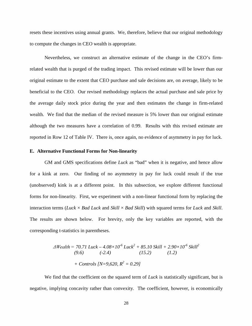
E. Alternative Functional Forms for Non-linearity

GM and GMS specifications define Luck as “bad” when it is negative, and hence allow

for a kink at zero. Our finding of no asymmetry in pay for luck could result if the true

(unobserved) kink is at a different point. In this subsection, we explore different functional

forms for non-linearity. First, we experiment with a non-linear functional form by replacing the

interaction terms (Luck × Bad Luck and Skill × Bad Skill) with squared terms for Luck and Skill.

The results are shown below. For brevity, only the key variables are reported, with the

corresponding t-statistics in parentheses.

ΔWealth = 70.71 Luck – 4.08×10-6 Luck2 + 85.10 Skill + 2.90×10-6 Skill2 (9.6) (-2.4) (15.2) (1.2) + Controls [N=9,620, R2 = 0.29]

We find that the coefficient on the squared term of Luck is statistically significant, but is

negative, implying concavity rather than convexity. The coefficient, however, is economically

29

insignificant: we find that the inflection point is larger than the highest possible value of Luck in

the sample, indicating that the relation between pay and luck is essentially linear.

Second, we estimate piecewise linear regressions (as in Morck, Shleifer, and Vishny

(1988)). We divide our sample into three equal-sized groups (terciles) based on Luck. We label

the breakpoints corresponding to the 33rd and 67th percentiles of Luck as Luck33 and Luck67. We

then define three variables:

(i) T1Luck = Luck if Luck < Luck33 = Luck33 if Luck ≥ Luck33 (ii) T2Luck = 0 if Luck < Luck33 = Luck – Luck33 if Luck33 ≤ Luck < Luck67 = Luck67 – Luck33 if Luck ≥ Luck67 (iii) T3Luck = 0 if Luck < Luck67 = Luck – Luck67 if Luck ≥ Luck67

We replace Luck and Luck × Bad Luck in the regressions with the three variables. The

coefficients on these three variables represent the pay for luck sensitivity over the relevant range.

Thus, the coefficient on T3Luck represents the pay for luck if luck is above the 67th percentile

value. Results are reported below. Again, for brevity, only the coefficients on the three

variables and the corresponding t-statistics are reported below.

ΔWealth = 71.19 T1Luck + 74.18 T2Luck + 71.61 T3Luck + Controls (N = 9,620; R2 = 0.29) (7.8) (9.8) (8.1)

All three coefficients are significantly positive, implying that there is pay for luck across

all levels of luck. If there is strong convexity, then the coefficient on T3Luck should be

significantly greater than the coefficient on T2Luck, and the coefficient on T2Luck should be

significantly greater than the coefficient on T1Luck. It is also possible that the relation between

pay and luck is weakly convex, where the kink might be only at one of the two breakpoints. We

30

find that none of the coefficients are significantly different from each other. Overall, we find no

evidence of asymmetry in pay for luck with either of our two non-linear specifications.

F. Do CEOs with Greater Power Exhibit Asymmetry in Pay for Luck?

If asymmetry in pay for luck is consistent with skimming, it is likely that it is more

pronounced in firms with more powerful CEOs. To examine this, for each year, we classify

CEOs as being powerful if their ownership in the firm is above the median ownership of all

CEOs, if board co-option is above the median, if their tenure is above the median CEO tenure, or

if they have the combined position of CEO and Chairman of the Board.23 Board co-option, as in

Coles, Daniel, and Naveen (2010), is defined as the ratio of the number of directors who are

appointed to the board after the executive becomes the CEO, divided by board size. Rows 13–16

of Table IV present the results. The coefficient on Luck × Bad Luck is insignificant for the last

three measures of CEO power. For the high-ownership subsample, the co-efficient is

significantly positive, which is opposite to what would be predicted by the skimming hypothesis

of GM. This implies that the decrease in CEO firm-related wealth in response to bad luck is

more in absolute terms compared to the increase in wealth in response to good luck.

Overall, the results indicate that, even for relatively powerful CEOs, the reward for good

luck is similar to the penalty for bad luck.

G. Alternative Measures of Governance

In Section III.B we show that there is no asymmetry in pay for luck in firms with weaker

governance. Here we consider alternative measures of governance: number of five percent

institutional blockholders (Bertrand and Mullainathan (2001)), institutional ownership (Hartzell

23 These measures are chosen based on studies such as Coles, Daniel, and Naveen (2010), Bertrand and Mullainathan (2001), Goyal and Park (2002), and Denis, Denis, and Sarin (1997).

31

and Starks (2003)), and the fraction of independent directors (Weisbach (1988)).24 If pay for

luck asymmetry is evidence of skimming, there should be more pay-for-luck asymmetry in firms

with fewer blockholders, lower institutional holding, or lower fraction of independent directors.

We classify firms as having low governance if they have below-median values of number of 5%

blockholders, institutional ownership, or fraction of independent directors. Rows 17–19 of Table

IV present the results. In all cases, the coefficient on Luck × Bad Luck is insignificant.

H. Inclusion of Firms with Non-December Fiscal Year Ends

Our base-case scenario, consistent with GM and GMS, excludes firms with non-

December fiscal year ends so that performance measures for all firms are compared over the

same time period. We re-estimate our key specification by including all firms. Row 20 of Table

IV reports the results. We find no evidence of asymmetry in pay for luck.

I. Median Regressions

Our primary regressions are based on OLS estimates, with the key variables winsorized at

the 1st and 99th percentiles to minimize the influence of any outliers. Our results are qualitatively

similar when we use median regressions (using unwinsorized values), as can be seen in Row 21

of Table IV. The coefficient on Luck × Bad Luck is again statistically insignificant.

J. Other Econometric Issues

Our specifications to this point include executive and year fixed effects with robust

standard errors. This is consistent with GM and GMS. We explore several alternative

econometric specifications, including: (i) the use of industry fixed effects rather than executive

fixed effects, (ii) the use of firm fixed effects rather than executive fixed effects, and (iii)

clustering the standard errors by firm, rather than using robust standard errors. Results are

24 Data on number of institutional blockholders and institutional holding is from Thomson Reuters.

32

reported in Rows 22–24. In both cases, we find no asymmetry in pay for luck.

Finally, we re-estimate our baseline regression with the values of Luck and Skill

winsorized at the 1st and 99th percentile values. As noted earlier, all variables that we use in our

regressions are winsorized. Luck and Skill, however, are the predicted and residual values from a

regression of firm returns on industry returns, where both firm and industry returns are already

winsorized, so we do not winsorize these variables. But Luck and Skill are both skewed, and we

therefore check whether our results are robust if we use winsorized values of Luck and Skill. As

can be seen from the results in Row 25, we continue to find no asymmetry in pay for luck.

Overall, the findings in this section support our key result: there is no asymmetry of pay

to luck when change in CEO firm-related wealth is used as the dependent variable.

V. Conclusions

Garvey and Milbourn (GM, 2006) and Gopalan, Milbourn, and Song (GMS, 2010)

document that CEOs’ annual pay increases in response to performance changes attributable to

good luck, but does not decrease as much in response to performance changes attributable to bad

luck. GM find this asymmetry to be stronger in firms with poor governance and argue that their

results are consistent with managerial rent extraction. GMS, on the other hand, argue that this

asymmetry is optimal for certain sets of firms.

Our point of departure from the GM and GMS studies is in using the change in the

CEO’s firm-related wealth rather than the change in annual pay or the level of annual pay. When

we use the change in the CEO’s firm-related wealth, we find no asymmetry in pay for luck.

Our use of change in firm-related wealth is based on Aggarwal and Samwick (1999), who

find that the sensitivity of CEO compensation to firm performance arising from the change in

pay or level of pay is only a small slice of the overall pay-for-performance sensitivity, and that

33

the major part of the pay-for-performance sensitivity is derived from the CEO’s stock and option

holdings. Our choice is also supported by early studies on ex-post pay-performance sensitivities

(Jensen and Murphy (1990), Hall and Liebman (1998), Aggarwal and Samwick (1999),

Himmelberg and Hubbard (2000), Milbourn (2003), Garvey and Milbourn (2003), and Rajgopal,

Shevlin, and Zamora (2006)), and on ex-ante pay-performance sensitivities (Core and Guay

(1999), Guay (1999), and Core and Guay (2002)).

GM argue that if asymmetry in pay for luck is consistent with skimming then it should be

more pronounced in firms with weaker governance. Using several proxies for governance, we

find no asymmetry in firms with weaker governance structures when we use changes in firm-

related wealth. Our findings do not imply, however, that there is no rent extraction by managers.

We can only conclude that rent extraction is not through asymmetry in pay for luck.

Additionally, we find no evidence in support of the predictions of the GMS model of optimal

contracting. A possible explanation is that the GMS assumptions in their theoretical model are

too stringent and are not supported in the data.

Our results also have relevance for studies that attribute certain governance structures as

weak or strong based on how the governance structure impacts pay-performance sensitivities.

Several studies (examples: Faleye (2007), Hwang and Kim (2009)) argue that lower pay-

performance sensitivities are associated with weaker governance structures, but these studies use

change in annual pay. Our study shows that the inferences may be quite different if pay-

performance sensitivities are based on change in wealth, rather than change in pay or level of

pay. Future work could explore this in more detail.

Finally, we make a methodological contribution in terms of computing more precisely the

change in the CEO’s firm-related wealth.

34

Appendix Methodology to Estimate Change in CEO’s Firm-Related Wealth:

Ours and Comparison with Current Literature We first elaborate on our methodology to estimate the change in the CEO’s firm-related wealth. We then compare our methodology with that followed by the current literature. Specifically, we discuss the 12 components that comprise our estimate of the change in CEO’s firm-related wealth, and discuss how each of these components would be treated by the current methodology. A1. Our Methodology to Estimate Change in Firm-Related Wealth Intuitively, the change in CEO’s firm-related wealth is given by:

∆ Firm-related wealth = ∆ Wealth from equity holdings and equity pay + Annual non-equity pay (1)

where equity includes both stocks and options. Specifically,

∆ Wealth from equity holdings and equity pay = ∆ Value of stock portfolio + ∆ Value of option portfolio + $ realized from CEO stock sales – $ paid by CEO for stock purchases – $ paid by CEO to exercise shares (2)

The last three components are estimated using insider trading data from Thomson Reuters. We first merge Execucomp with Thomson Reuters using the 6-digit historical CUSIP. Because the historical CUSIP is not a unique identifier and is subject to change over time, we then manually check the merged file using CEO names to ensure the validity of the matching.25

Annual non-equity pay = Total pay – Value of shares granted – Value of options granted (3)

Total pay is given by the ExecuComp variable TDC1. If data were reported in the old format (ExecuComp variable OLD_DATAFMT_FLAG=1) then the value of shares granted is given by ExecuComp variable “RSTKGRNT” and the value of options granted is given by ExecuComp variable “OPTION_AWARDS_BLK_VALUE.” If data were reported in the new format (ExecuComp variable OLD_DATAFMT_FLAG=0) then the value of shares granted is given by ExecuComp variable “STOCK_AWARDS_FV” and the value of options granted is given by ExecuComp variable “OPTION_AWARDS_FV.” In the year 2006, 15% of firms reported in the old format. Before 2006, all firms reported in the old format, and after 2006 all firms reported in the new format. 25 We include all trades reported in form 4 and 5, except ones with transaction codes of “9” or “A”, where “9” stands for invalid trades due to reporting errors, and “A” stands for grants and awards. Buy or sale is determined by the acquisition/disposal code (variable “ACQDISP”).

35

We illustrate our methodology using a hypothetical example.

Let S indicate the number of shares, O indicate the number of options, P indicate stock price, and V indicate option value. The subscripts denote time periods or specific tranches of securities. Let b indicate beginning-of-year, e indicate end-of-year, g indicate securities granted by the board during the year, x indicate securities involved in option exercise by the executive, p indicate shares purchased by the executive during the year, s indicate shares sold by the executive during the year, r indicate options repriced, and exp indicate options that expired out of the money. The table below tabulates the notation used to denote the number of shares of each type and the share price relevant for each type of shares.

Number Price at beginning-of-year

Event Price

Price at end-of-year

Shares held at the beginning of the year Sb Pb

Shares held at the beginning of the year that remain at the end of the year

Sh Pb Pe

Shares granted during the year Sg Pg Pe

Shares obtained from option exercise Sx Px Pe

Shares purchased during the year Sp Pp Pe

Shares sold during the year26 Ss Pb Ps

Shares at end of the year Se Pe

Assume Sb = 1000; Sg = 300; Sx = 100; Sp = 200; and Ss = 400. Then Se = Sb + Sg + Sx + Sp – Ss = 1000 + 300 + 100 + 200 – 400 = 1200. For illustration purpose, we assume that the 400 shares sold were from the shares held at the beginning of the year.27 That is, Sh = Sb – Ss = 1000 – 400 = 600. The table below tabulates the notation used to denote the number of options of each type and value of each option type for the relevant time period. The first subscript denotes the type of option and the second subscript denotes the time.28 26 As discussed earlier, this includes shares given to charity as gifts by the CEOs because the intent of usage of the funds realized from stock sale should not impact our estimate of firm-related wealth. 27 The final estimate of change in firm-related wealth remains the same if instead we assume that some of the shares sold were from the shares obtained during the year from option exercise. See next footnote for details. 28 This representation is for simplicity only. In reality the portfolio consists of many tranches, each with its own exercise price. Post-2006, we estimate the option value for each tranche using the exercise price for that tranche and then sum up the option values of each tranche to obtain the portfolio value of the option holdings.

36

Number Value at beginning-of-year

Value at grant date

Value at end-of-year

Options held at the beginning of the year that remain at the end of the year

Oh Vh,b Vh,e

Options expired during the year Oexp Vexp,b 0

Options repriced during the year Or Vr,b Vr,e

Options exercised during the year Ox Vx,b NA

Options granted during the year Og Vg,g Vg,e

Assume Ob = 2000; Oexp = 200; Ox = Sx = 100; Og = 500; Or = 300; Then Oe = Ob – Oexp – Ox + Og = 2000 – 200 – 100 + 500 = 2200. Then Oh = Ob – Oexp – Ox – Or = 2000 – 200 – 100 – 300 = 1400. Our estimate of change in CEO’s firm-related wealth is given by the summation of (4) – (8) below.

∆ Value of stock portfolio = 1200×Pe – 1000×Pb (4)

∆ Value of option portfolio = (1400×Vh,e + 300×Vr,e + 500×Vg,e) – (1400×Vh,b + 300×Vr,b + 200×Vexp,b + 100×Vx,b) (5)

We are assuming here that, with repriced options, only the exercise price is altered. It is possible that firms alter other terms such as number of options. This will not affect our estimate of change in CEO firm-related wealth because, in practice, we estimate only the change in value, which takes into account both the number of options and per-option value. Repricing, however, is not very common. Hence even though our methodology takes it into account it will not lead to a substantive difference in our estimate of change in CEO firm-related wealth.

$ realized from CEO stock sales = 400×Ps (6) $ paid by CEO for stock purchases = – 200×Pp (7) $ paid by CEO to exercise options = – 100×Px (8)

We do not have to explicitly adjust for stock splits here as we are interested in the value (number of shares × share price) and any difference in number of shares due to split adjustment will be offset by the difference in share prices. A2. Comparison of Methodologies: Ours Vs. Current Literature The current methodology computes change in firm-related wealth as follows:

37

∆ Firm-related wealth = ∆ Wealth from beginning-of-year equity holdings + Value of annual equity grants + Annual non-equity pay (9)

where change in wealth is estimated by multiplying the starting portfolio of stock and options by the corresponding change in the value of stock and options during the year. As stated in the introduction, this method ignores (i) stock sales by the CEO, (ii) stock purchases by the CEO, (iii) option exercises by the CEO and the resultant loss in time value of options from exercising them before maturity, (iv) option repricing, (v) options expiring out-of-the-money, and (vi) any change in value in the equity grants from the grant date to the fiscal year end date. Below, we break up the change in firm-related wealth as estimated by us into 12 components so that we can readily see the methodological improvements we make compared to prior literature. (i) Change in wealth due to 600 shares that were in the portfolio at the beginning of the year

and continue to be held in the portfolio at the end of the year = 600×(Pe–Pb). The current methodology correctly estimates this component.

(ii) Change in wealth due to 400 shares that were sold during the year = 400×(Ps–Pb).

Current methodology assumes that these 400 shares stay in the portfolio till the end of the year, and hence estimates this component as 400×(Pe–Pb). Part of the sales is pre-planned sales (10b5-1 filing) sold on some randomly chosen date by the executive. This should carry no information and hence, by definition, the sale price (Ps) is not expected to be systematically different from year-end-price (Pe). The other part of the sales could be trades based on information. This should be advantageous to the executive and hence Ps is expected to be greater than Pe. Putting both the sales together, Ps, on average, is expected to be greater than Pe, and hence current methodology underestimates the true wealth change.

(iii) Change in wealth due to 300 shares that were granted during the year = 300×Pg.

The current methodology correctly estimates this component.

(iv) Change in wealth associated with the 300-share grant from the time of grant to the end of

the year = 300×(Pe–Pg).

The current methodology does not consider this component at all. Given the evidence on timing of equity grants (Yermack (1997)), we expect that, on average, Pe will be greater than Pg, and hence current methodology underestimates the true wealth change.

(v) Change in wealth due to 200 shares that were bought during the year = 200×(Pe–Pp).

The current methodology does not consider this component at all. Given that insider purchases are typically associated with positive abnormal return, we expect, on average,

38

year-end price (Pe) to be greater than purchase price (Pp). Thus, the current methodology underestimates the true wealth change.

(vi) Change in wealth due to 1400 options that were in the portfolio at the beginning of the

year and continues to be there in the portfolio at the end of the year = 1400×(Vh,e–Vh,b). The current methodology correctly estimates this component.

(vii) Change in wealth due to 300 options that were repriced = 300×Vr,e – 300×Vr,b.

The current methodology does not allow for option repricing, and hence considers the change in value of repriced options based on the initial terms of the option, and not based on the adjusted or repriced terms. Since repricing typically results in higher value post-repricing, current methodology underestimates the true wealth change.

(viii) Change in wealth due to 200 options that expired out of the money = –200×Vexp,b.

The current methodology does not allow for option expiry, but assumes these options are held in the portfolio till the end of the year, and hence overestimates the true wealth change.

(ix) Change in wealth due to 100 options that were exercised and continue to remain in the portfolio as shares = 100×Pe – 100×Vx,b – 100×Px. The current methodology does not assume any option exercise and hence assumes these options remain in the portfolio at the end of the year. Thus, the change in wealth from this component is estimated wrongly as 100×Vx,e – 100×Vx,b. When the CEO exercises early, he loses the time value of the option. But he may gain if the share price appreciates after option exercise because stocks, compared to options, have higher sensitivity to stock price. Thus, it is not clear whether the current methodology underestimates or overestimates the true wealth change.

(x) Change in wealth due to 500 options that were granted during the year = 500×Vg,g. The current methodology correctly estimates this component.

(xi) Change in wealth associated with the 500-option grant from the time of grant to the end

of the year = 500×(Vg,e–Vg,g). The current methodology does not consider this component at all. Given the evidence on timing of equity grants (Yermack (1997)), we expect that, on average, Vg,e will be greater than Vg,g, and hence current methodology underestimates the true wealth change.

(xii) Change in wealth from non-equity pay. The current methodology correctly estimates this component.

39

The change in CEO’s firm-related wealth from equity holdings and equity pay is the summation of the 12 components, and simplifies to the following29:

∆ Firm-Related Wealth = (1200×Pe – 1000×Pb)

+ (1400×Vh,e + 300×Vr,e + 500×Vg,e) – (1400×Vh,b + 300×Vr,b + 200×Vexp,b + 100×Vx,b) + (400×Ps) – (200×Pp) – (100×Px) + Non-equity pay (10) The current methodology correctly estimates five components, underestimates five components, overestimates one component, and it is not possible to judge ex-ante for one component. Thus ex-ante one cannot categorically say whether the current methodology will underestimate or overestimate the true wealth change.

29 If we had assumed that, say, 25 out of the 400 shares sold were obtained from option exercise. Then 375 shares sold are from the beginning-of-year holdings and hence 625 of the beginning-of-year holdings remain in the holdings at the end of the year. Now only the 1st, 2nd, and 9th components are affected as follows. The other components remain exactly the same, though the summation of the 12 components still yield the same value. • Change in wealth due to 625 shares that were in the portfolio at the beginning of the year and continue to be

there in the portfolio at the end of the year = 625×(Pe–Pb). • Change in wealth due to 375 shares that were sold during the year = 375×(Ps–Pb). The 25 shares that were

obtained from option exercise and sold during the year are considered below. • Change in wealth due to 100 options that were exercised, of which 75 continue to remain in the portfolio as

shares and 25 was sold during the year = 75×Pe + 25×Ps – 100×Vx,b – 100×Px.

40

References

Aggarwal, R.K., and A. A. Samwick. 1999. The Other Side of the Trade-Off: The Impact of Risk on Executive Compensation. Journal of Political Economy 107: 65-105.

Bertrand, M., and S. Mullainathan. 2001. Are CEOs Rewarded for Luck? The Ones without Principals Are. Quarterly Journal of Economics 116: 901-932.

Bizjak J. M., M. L. Lemmon, and L. Naveen. 2008. Does the Use of Peer Groups Contribute to Higher Pay and Less Efficient Compensation? Journal of Financial Economics 90: 152-168.

Carhart, M. . 1997. On Persistence in Mutual Fund Performance. Journal of Finance 52: 57-82. Coles, J. L., N. D. Daniel, and L. Naveen. 2006. Managerial Incentives and Risk-Taking. Journal

of Financial Economics 79: 431-468. Coles, J. L., N. D. Daniel, and L. Naveen. 2010. Co-opted Boards. Working Paper, Arizona State

University, Drexel University, and Temple University. Core J., and W. Guay. 1999. The Use of Equity Grants to Manage Optimal Equity Incentive

Levels. Journal of Accounting and Economics 28: 151-184. Core J., and W. Guay. 2002. Estimating the Value of Employee Stock Option Portfolios and

Their Sensitivities to Price and Volatility. Journal of Accounting Research 40: 613-630. Denis, D., Denis, J., and A. Sarin, 1997. Ownership Structure and Top Executive Turnover.

Journal of Financial Economics 45: 193-221. Fahlenbrach, R., and R. Stulz, 2011. Bank CEO Incentives and the Credit Crisis. Journal of

Financial Economics 99: 11-26. Faleye O., 2007. Classified Boards, Firm Value, and Managerial Entrenchment. Journal of

Financial Economics 83: 501-529. Fama, E., and K. French, 1993. Common Risk Factors in the Returns on Stocks and Bonds.

Journal of Financial Economics 33: 3-56. Frydman, C., and D. Jenter, 2010. CEO Compensation. Annual Review of Financial Economics.

2: 103-125. Garvey, G., and T. Milbourn. 2003. Incentive Compensation When Executives Can Hedge the

Market: Evidence of Relative Performance Evaluation in the Cross Section. Journal of Finance 58: 1557-1581.

Garvey, G., and T. Milbourn. 2006. Asymmetric Benchmarking in Compensation: Executives Are Rewarded for Good Luck But Not Penalized for Bad. Journal of Financial Economics 82: 197-225.

Gibbons, R., and K. J. Murphy, 1990. Releative Performance Evaluation for Chief Executive Officers. Industrial and Labor Relations 43: 30S-51S.

Gompers P., J. Ishii, and A. Metrick. 2003. Corporate Governance and Equity Prices. The Quarterly Journal of Economics 118: 107-156.

Gopalan R., T. Milbourn, and F. Song. 2010. Strategic Flexibility and the Optimality of Pay for Sector Performance. Review of Financial Studies 23: 2060-2098.

Goyal, V., and C. Park. 2002. Board leadership structure and CEO turnover. Journal of Corporate Finance 8: 49-66.

Guay W. 1999. The Sensitivity of CEO Wealth to Equity Risk: An Analysis of the Magnitude and Determinants. Journal of Financial Economics 53: 319-351.

Hall, B. J., and J. B. Liebman. 1998. Are CEOs Really Paid Like Bureaucrats? Quarterly journal of Economics 113: 653-692.

41

Harford, J., and K. Li, 2007. Decoupling CEO Wealth and Firm Performance: The Case of Acquiring CEOs. Journal of Finance 62: 917-949.

Hartzell J. C., and L. T. Starks. 2003. Institutional Investors and Executive Compensation. Journal of Finance 58: 2351-2374.

Himmelberg, C., and G. Hubbard. 2000. Incentive Pay and the Market for CEOs: An analysis of Pay-for-Performance Sensitivity. Working paper, Columbia University.

Hwang B., and S. Kim. 2009. It Pays to Have Friends. Journal of Financial Economics 93: 138-158.

Jensen, M. C., and K. J. Murphy. 1990. Performance Pay and Top-Management Incentives. Journal of Political Economy 98: 225-264.

Merton, R., 1973. Theory of rational option pricing. Bell Journal of Economics and Management Science 4, 141–183.

Morck, R., Shleifer, A., Vishny, R., 1988. Management Ownership and Market Valuation: an Empirical Analysis. Journal of Financial Economics 20: 293–315.

Milbourn, T. 2003. CEO Reputation and Stock-based Compensation. Journal of Financial Economics 68: 233-263.

Murphy, K. J., 1985. Corporate Performance and Managerial Remuneration: An Empirical Investigation. Journal of Accounting and Economics 7: 11-42.

Petersen, M., 2009. Estimating Standard Errors in Finance Panel Data Sets: Comparing Approaches. Review of Financial Studies 22: 435-480.

Rajgopal S., and T. Shevlin. 2002. Empirical Evidence on the Relation between Stock Option Compensation and Risk Taking. Journal of Accounting and Economics 33: 145-171.

Rajgopal S., and T. Shevlin, and V. Zamora, 2006. CEO’s Outside Employment Opportunities and Lack of Relative Performance Evaluation, Journal of Finance 61: 1813-1844.

Weisbach, M., 1988. Outside Directors and CEO Turnover. Journal of Financial Economics 20: 421-460.

Yermack, D., 1997. Good Timing: CEO Stock Option Awards and Company News Announcements. Journal of Finance 52: 449-476.

Yermack, D., 2009a. Deductio Ad Absurdum: CEOs Donating Their Own Stock to Their Own Family Foundations. Journal of Financial Economics 94: 107-123.

Yermack, D., 2009b. Keeping the Pay Police at Bay. Wall Street Journal (10/10/2009).

42

Table I Descriptive Statistics

The table provides descriptive statistics on Chief Executive Officer (CEO) compensation and CEO and firm characteristics for the sample period 1992-2005. Compensation data are from ExecuComp, stock return data are from CRSP, accounting data are from Compustat, and insider trading data are from Thomson Reuters. Level of Pay is the ExecuComp variable TDC1 and includes salary, bonus, total value of stock and option grants, long term incentive payouts, other annual compensation, and all other compensation. Change in Pay is pay of current year less pay of prior year. Change in Firm-related Wealth is the change in value of the stock portfolio + change in value of the option portfolio + dollar value of shares sold during year – dollar value of shares purchased during year – dollars spent on options exercised during year + non-equity pay. Value of Stock Portfolio = number of shares held by the CEO at the end of the year × share price at the end of the year. Value of Option Portfolio is the Black-Scholes value of options at the end of the year. Non-equity Pay is the total pay – value of stocks granted – value of options granted. Dollar Return is the annual stock return multiplied by the firm’s lagged market capitalization. We estimate a regression of annual stock returns on the value-weighted and equal-weighted industry (2-digit SIC) returns. We (i) do not include the firm’s returns in the industry returns, (ii) do not include an intercept term, and (iii) eliminate all firms that do not have a December fiscal-year end to ensure that the performance measures for all firms are over the same time period and hence comparable. Luck is the predicted value multiplied by the lagged market capitalization of the firm and Skill is the residual value multiplied by the lagged market capitalization of the firm. As in Garvey and Milbourn (2006), only CEOs with two consecutive years of coverage are included.

Panel A: Firm and CEO characteristics

Obs Mean Median

Sales ($M) 13,087 3,797 1,063

Level of Pay ($000s) 12,892 3,829 1,998

Value of Stock + Option Portfolio ($000s) 11,803 61,901 16,625

Change in Pay ($000s) 11,780 213 126

Change in Value of Stock + Option Portfolio ($000s) 10,202 7,687 1,445

Non-equity Pay ($000s) 12,892 1,777 1,065

Change in Firm-related Wealth ($000s) 10,218 11,307 3,127

Dollar Return ($M) 13,090 548 104

Luck ($M) 13,028 977 136

Skill ($M) 13,028 (398) (30)

CEO Tenure (years) 12,551 8 6

Panel B: Correlations

Change in Firm-related Wealth Change in Pay Level of Pay Change in Firm-related Wealth 1.00 Change in Pay 0.16 1.00 Level of Pay 0.23 0.43 1.00

43

Table II Tests of Asymmetry in Pay for Luck

The table reports results from OLS regressions of change in pay, level of pay, and change in the firm-related wealth. Compensation variables are defined in Table I. We estimate a regression of annual stock returns on the value-weighted and equal-weighted industry (2-digit SIC) returns. We (i) do not include the firm’s returns in the industry returns, (ii) do not include an intercept term, and (iii) eliminate all firms that do not have a December fiscal-year end to ensure that the performance measures for all firms are over the same time period and hence comparable. Luck is the predicted value multiplied by the lagged market capitalization of the firm and Skill is the residual value multiplied by the lagged market capitalization of the firm. Bad Luck is an indicator variable that equals 1 when Luck ≤ 0, and equals 0 otherwise. Bad Skill is an indicator variable that equals 1 when Skill ≤ 0, and equals 0 otherwise. cdf Variance of Luck and cdf Variance of Skill are estimated using rolling 5 year windows. “GM” refers to Garvey and Milbourn (2006) and “GMS” refers to Gopalan, Milbourn, and Song (2010). Intercept, year, and executive fixed effects are included in the model. t-statistics are based on robust standard errors. ***, **, and * represent significance at the 1%, 5%, and 10% levels.

Dependent Variable Change in Pay:

GM (1)

Level of Pay: GMS

(2)

Change in firm-related wealth

(3)

Luck 1.35** 2.02*** 72.77*** (2.5) (4.3) (10.0)

Skill 2.03*** 1.37*** 85.23*** (6.5) (5.7) (15.2)

Luck × Bad Luck -0.19** -0.28*** -0.002 (-2.5) (-2.6) (-0.0)

Skill × Bad Skill 0.01 -0.18*** -0.80 (0.2) (-3.7) (-1.6)

Luck × cdf Variance of Luck -1.30** -1.96*** -71.12*** (-2.4) (-4.1) (-9.7)

Skill × cdf Variance of Skill -2.01*** -1.25*** -83.02*** (-6.4) (-5.2) (-14.7)

cdf Variance of Luck -400.26 2,172.63*** 6,268.00 (-1.0) (4.3) (1.1)

cdf Variance of Skill -93.70 1,073.09*** 1,840.79 (-0.3) (2.6) (0.3)

CEO Tenure -0.78 283.66*** 3,031.11 (-0.0) (2.6) (1.5)

Observations 10,824 11,002 9,620 R2 0.02 0.13 0.29

44

Table III Asymmetry in Pay for Luck: Subsample Analysis as in GM and GMS

The table reports results from Model 3 of Table II (Base-Case Specification) for various subsamples of firms. For ease of presentation, only the coefficients on Luck, Luck × Bad Luck, and Luck × cdf Variance of Luck are reported. Compensation and firm performance measures are defined in Tables I and II. Weak Governance Firms are those for whom Gompers-Ishii-Metrick (2003) index value ≥ 12. Diversified Firms are those that operate in more than one business segment. As in GMS, we define firms in industries with high market-to-book ratios and firms in industries with high R&D/Assets ratio as having greater strategic flexibility. High Market-to-Book Firms are firms in industries whose median market-to-book ratio is above the 60th percentile of the overall market-to-book ratio. High R&D-to-Assets Firms are firms in industries whose median R&D-to-assets ratio is above the 70th percentile of overall R&D-to-assets ratio. As in GMS, High Returns Firms and Outsider CEO Firms are those managed by talented CEOs. High Returns Firms are those with above-median industry-adjusted returns. Outsider CEO Firms are those where the CEO when appointed came from outside the firm. t-statistics are based on robust standard errors. ***, **, and * represent significance at the 1%, 5%, and 10% levels.

Row Subsample

Coefficient

N R2 Luck Luck ×

Bad Luck Luck ×

cdf Variance of Luck

(0) Base-Case Specification

72.77*** -0.002 -71.12*** 9,620 0.29 (10.0) (0.0) (-9.7)

(1) Weak Governance Firms

41.80*** -1.81 -40.58*** 1,753 0.25 (3.6) (-0.5) (-3.4)

(2) Diversified Firms

89.78*** -0.98 -87.91*** 4,690 0.31 (7.8) (-0.9) (-7.6)

(3) High Market-to-Book Firms

84.41*** -0.70 -83.12*** 3,651 0.32 (6.4) (-0.3) (-6.3)

(4) High R&D-to-Assets Firms

75.26*** 0.16 -74.45*** 2,662 0.39 (5.0) (0.2) (-4.9)

(5) High Returns Firms

79.93*** -0.63 -78.08*** 4,719 0.30 (7.2) (-0.2) (-7.0)

(6) Outsider CEO Firms

111.54*** 1.69 -109.42*** 2,174 0.38 (6.0) (0.8) (-5.8)

45

Table IV Lack of Asymmetry in Pay for Luck: Robustness

The table reports results from Model 3 of Table II (Base-Case Specification) for alternative subsamples of firms and alternative specifications. We focus on the coefficient on Luck × Bad Luck to test for asymmetry in pay for luck. We also report the coefficients on Luck × Bad Luck and Luck × cdf Variance of Luck so that an interested reader can easily see that the asymmetry in pay for luck is never economically significant. Compensation and firm performance measures are defined in Tables I and II. 2007–2010 subsample includes only the years 2007 to 2010. Positive Returns subsample includes only the firm-years where annual returns are positive. Option Ratio is defined as the value of the option portfolio divided by CEO’s firm-related wealth, where wealth equals the value of stock portfolio plus the value of option portfolio plus non-equity pay. Moneyness is defined as the ratio of fiscal year end stock price to the average exercise price of the option portfolio. Maturity is the weighted average maturity of the option portfolio with the weights being the number of options in each tranche. This is estimated only for the 2007-2010 period. $ Wealth Change on Luck Estimated as Rate of Return specification uses change in CEO’s firm-related wealth as the dependent variable and Luck and Skill (expressed as rates of return) as independent variables. Luck and Skill are the predicted and residual values from a regression of firm returns on equal-weighted and value-weighted industry returns with an intercept included to ensure that the correlation between residual and predicted values is zero. These values are not scaled by the firm’s lagged market capitalization. Rate of Wealth Change on Luck Estimated as Rate of Return specification is exactly the same as earlier, but the dependent variable is the rate of change in firm-related wealth, which is defined as change in CEO’s firm-related wealth divided by lagged CEO’s firm-related wealth. For the Luck Estimated with Dollar Returns specification, Luck and Skill are the residual and predicted values from a regression of the firm’s dollar return on the dollar industry return (includes an intercept), where the firm’s dollar return is the firm’s annual rate of return multiplied by the firm’s lagged market capitalization, and the dollar industry return is the average dollar returns of all firms in the industry to which the firm belongs excluding the firm’s own dollar return. Luck = Average Returns minus Carhart Alpha specification uses Carhart Alpha as a proxy for Skill. Carhart Alpha is the intercept from a time-series regression of daily excess returns on the daily factors of Fama and French (1993) and the momentum factor of Carhart (1997). Luck is average excess return less the Carhart Alpha. To avoid look-ahead bias and estimate observable luck and skill, the regression is estimated each year using daily returns for the same year for which CEO’s firm-related wealth is calculated. We annualize the measures by multiplying Luck and Skill by 250. Wealth Change Based on Prior Literature specification uses change in wealth estimated as per prior literature. This is obtained by multiplying the starting portfolio of stock and options by the change in value of stock and options during the year and then adding the annual pay (which includes the value of annual equity grants). Wealth Change Purged of CEO Influence specification uses wealth change estimated as per our methodology but replaces the price at which CEO purchased and sold stocks by the average stock price during the year in which the purchase and sales were made. High CEO Ownership subsample includes firms whose CEO stock ownership is above the median value. High Board Co-option subsample includes firms whose board co-option is above the median value. Board co-option is the number of directors who joined the board after the executive became CEO divided by the board size. High CEO Tenure subsample includes firms whose CEO tenure is above the median value. CEO-Chairman Duality subsample includes firms where the CEO is also the Chairman of the board. Low Blockholding subsample includes firms for whom the number of 5% institutional block holders is lower than the median value. Low Institutional Ownership subsample includes firms for whom the total institutional ownership is lower than the median value. Blockholders data and institutional ownership data are from Thomson Reuters. Low Fraction Independent Directors subsample includes firms where the fraction of independent directors is below the median value. Winsorized Luck and Skill specification uses winsorized values of Luck and Skill. t-statistics are based on robust standard errors. The R2 reported for the median regressions is the pseudo R2. ***, **, and * represent significance at the 1%, 5%, and 10% levels.

46

Row Subsample Coefficient N R2

Luck Luck × Bad Luck

Luck × cdf variance of Luck

(0) Base-Case Specification

(Model 3, Table II) 72.77*** -0.002 -71.12*** 9,620 0.29 (10.0) (0.0) (-9.7)

Core and Guay Methodology (1) 2007–2010 47.05*** 0.79 -46.76*** 3,772 0.30

(7.9) (1.6) (-7.8)

(2) Positive Returns

63.83*** 0.07 -61.75*** 6,210 0.22 (8.9) (0.0) (-8.4)

Impact of Option Compensation (3) Option Ratio > 80th percentile

46.64*** 1.66 -45.01*** 1,926 0.41 (4.0) (1.0) (-3.8)

(4) 0.8 < Moneyness < 1.2 for 2007-2010

19.67*** -1.95 -16.46** 913 0.30 (3.2) (-0.9) (-2.4)

(5) 0.8 < Moneyness < 1.2 for 1992-2005

32.30*** -0.33 -31.57*** 1,792 0.17 (3.1) (-0.6) (-3.0)

(6) Maturity < 20th percentile

79.92*** 1.61 -80.29*** 591 0.40 (5.6) (1.3) (-5.6)

Alternative Measures of Luck and Alternative Specifications for PPS

(7) $ Wealth Change on Luck Estimated as Rate of Return

78,056.00*** -19,889.84 -17,124.06 9,620 0.20 (8.1) (-1.1) (-1.5)

(8)

Rate of Wealth Change on Luck Estimated as Rate of Return

1.75*** -0.05 -0.25 9,595 0.49 (11.2) (-0.2) (-1.4)

(9) Luck Estimated with Dollar Returns 26.69*** -4.37 -9.65 9,620 0.25 (4.8) (-1.2) (-1.6)

(10) Luck = Avg. Returns – Carhart Alpha

2.06*** 0.02 -0.34 9,622 0.44 (10.9) (0.1) (-1.6)

Alternative Definitions of Change in Wealth

(11) Wealth Change Based on Prior Literature

75.13*** -0.06 -73.27*** 9,527 0.37 (10.1) (-0.1) (-9.7)

(12) Wealth Change Purged of CEO Influence

72.99*** 0.02 -71.33*** 9,620 0.29 (10.0) (0.0) (-9.7)

CEO Power (13) High CEO Ownership

144.35*** 7.61*** -139.33*** 4,687 0.47 (10.1) (4.5) (-9.6)

(14) High Board Co-option

88.65*** -0.86 -85.74*** 3,052 0.39 (6.6) (-0.6) (-6.3)

(15) High CEO Tenure

90.00*** 1.29 -87.66*** 4,993 0.35 (8.6) (0.5) (-8.3)

(16) CEO-Chairman Duality

70.53*** 1.24 -69.07*** 6,218 0.29 (7.8) (0.7) (-7.6)

47

Row Subsample

Coefficient on:

N R2 Luck Luck × Bad Luck

Luck × cdf variance of Luck

Alternative Measures of Governance (17) Low Blockholding

63.99*** -0.35 -62.78*** 4,827 0.28 (7.3) (-0.4) (-7.1)

(18) Low Institutional Ownership

82.16*** 0.59 -81.18*** 3,571 0.28 (6.4) (0.8) (-6.3)

(19) Low Fraction Independent Directors

109.61*** -1.00 -107.25*** 3,239 0.37 (7.8) (-0.4) (-7.5)

Other Robustness

(20) Non-December Fiscal Year Ends Included

84.03*** 0.90 -82.70*** 14,323 0.28 (10.5) (0.7) (-10.3)

(21) Median Regressions 29.99*** 0.03 -28.63*** 9,620 0.18 (68.3) (0.6) (-64.9)

(22) Industry Fixed Effects 63.03*** -0.15 -61.41*** 9,620 0.29 (11.3) (-0.2) (-10.9)

(23) Firm Fixed Effects 63.79*** -0.01 -62.07*** 9,620 0.26 (9.3) (-0.0) (-9.0)

(24) Standard Errors Clustered by Firm

62.08*** -0.37 -60.41*** 9,620 0.27 (10.5) (-0.6) (-10.0)

(25) Winsorized Luck and Skill

56.15*** 7.13 -52.71*** 9,620 0.27 (7.5) (1.4) (-6.8)