ORNL/TM-2011/461

NMOG Emissions Characterizations and Estimation for Vehicles Using Ethanol-Blended Fuels

October 15, 2011 Prepared by

C. Scott Sluder Brian H. West

DOCUMENT AVAILABILITY Reports produced after January 1, 1996, are generally available free via the U.S. Department of Energy (DOE) Information Bridge. Web site http://www.osti.gov/bridge Reports produced before January 1, 1996, may be purchased by members of the public from the following source. National Technical Information Service 5285 Port Royal Road Springfield, VA 22161 Telephone 703-605-6000 (1-800-553-6847) TDD 703-487-4639 Fax 703-605-6900 E-mail info@ntis.gov Web site http://www.ntis.gov/support/ordernowabout.htm Reports are available to DOE employees, DOE contractors, Energy Technology Data Exchange (ETDE) representatives, and International Nuclear Information System (INIS) representatives from the following source. Office of Scientific and Technical Information P.O. Box 62 Oak Ridge, TN 37831 Telephone 865-576-8401 Fax 865-576-5728 E-mail reports@osti.gov Web site http://www.osti.gov/contact.html

This report was prepared as an account of work sponsored by an agency of the United States Government. Neither the United States Government nor any agency thereof, nor any of their employees, makes any warranty, express or implied, or assumes any legal liability or responsibility for the accuracy, completeness, or usefulness of any information, apparatus, product, or process disclosed, or represents that its use would not infringe privately owned rights. Reference herein to any specific commercial product, process, or service by trade name, trademark, manufacturer, or otherwise, does not necessarily constitute or imply its endorsement, recommendation, or favoring by the United States Government or any agency thereof. The views and opinions of authors expressed herein do not necessarily state or reflect those of the United States Government or any agency thereof.

ORNL/TM-2011/461

Fuels, Engines, and Emissions Research Center

NMOG Emissions Characterizations and Estimation for Vehicles Using Ethanol-Blended Fuels

Author(s) C. Scott Sluder Brian H. West

Date Published: October 15, 2011

Prepared by OAK RIDGE NATIONAL LABORATORY

Oak Ridge, Tennessee 37831-6283 managed by

UT-BATTELLE, LLC for the

U.S. DEPARTMENT OF ENERGY under contract DE-AC05-00OR22725

iii

CONTENTS

CONTENTS ....................................................................................................................................... iii LIST OF FIGURES ............................................................................................................................ v LIST OF TABLES ............................................................................................................................ vii ABSTRACT ........................................................................................................................................ 1 1. INTRODUCTION ........................................................................................................................ 2 2. EXPERIMENTAL DATA ........................................................................................................... 4

2.1 OHC Speciation Results ..................................................................................................... 5 3. ESTIMATING NMOG EMISSIONS .......................................................................................... 8

3.1 Estimation Procedure .......................................................................................................... 8 3.2 Results for Estimates of FTP Composite NMOG Emissions ........................................... 10 3.3 Estimates for Individual Phases of the FTP ...................................................................... 12 3.4 Correlation Validation with Additional Vehciles, Cycles, and Fuels ............................... 14 3.5 NMOG Measurement Considerations .............................................................................. 16

4. CONCLUSIONS ........................................................................................................................ 18 5. REFERENCES ........................................................................................................................... 19

v

LIST OF FIGURES

Figure Page Figure 1. Relative contributions of individual species to total bag 1 OHC emissions. ................................ 6 Figure 2. Bag 1 formaldehyde emissions. .................................................................................................... 7 Figure 3. Bag 1 acetaldehyde emissions. ..................................................................................................... 7 Figure 4. Composite NMOG vs NMHC emissions data for FTP tests conducted at TRC. ......................... 9 Figure 5. Composite NMOG vs NMHC emissions data for FTP tests conducted at SwRI. ........................ 9 Figure 6. NMOG/NMHC ratio regression with average fuel ethanol content. .......................................... 10 Figure 7. Estimated versus measured FTP composite NMOG emissions results. ..................................... 11 Figure 8. Histogram of the errors in the estimated FTP composite NMOG results. .................................. 11 Figure 9. Regression of NMOG/NMHC ratios to fuel ethanol blend level for FTP bag 2. ....................... 12 Figure 10. Regression of NMOG/NMHC ratios to fuel ethanol blend level for FTP bag 2. ..................... 13 Figure 11. Measured and estimated NMOG emissions for additional cycles. Columns represent the median result; range bars show the maximum and minimum results. ........................................................ 15 Figure 12. Comparison of estimated and measured FTP composite NMOG emissions for two vehicles using non-certification fuels. ...................................................................................................................... 16

LIST OF TABLES

Table Page

Table 1. Vehicle models included in the reported study. ............................................................................. 4 Table 2. Correlation constants and error bands for FTP bag-specific correlations. ................................... 14

1

ABSTRACT

Ethanol is a biofuel commonly used in gasoline blends to displace petroleum consumption; its utilization is on the rise in the United States, spurred by the biofuel utilization mandates put in place by the Energy Independence and Security Act of 2007 (EISA). The United States Environmental Protection Agency (EPA) has the statutory responsibility to implement the EISA mandates through the promulgation of the Renewable Fuel Standard. EPA has historically mandated an emissions certification fuel specification that calls for ethanol-free fuel, except for the certification of flex-fuel vehicles. However, since the U.S. gasoline marketplace is now virtually saturated with E10, some organizations have suggested that inclusion of ethanol in emissions certification fuels would be appropriate. The test methodologies and calculations contained in the Code of Federal Regulations for gasoline-fueled vehicles have been developed with the presumption that the certification fuel does not contain ethanol; thus, a number of technical issues would require resolution before such a change could be accomplished. This report makes use of the considerable data gathered during the mid-level blends testing program to investigate one such issue: estimation of non-methane organic gas (NMOG) emissions. The data reported in this paper were gathered from over 600 cold-start Federal Test Procedure (FTP) tests conducted on 68 vehicles representing 21 models from model year 2000 to 2009. Most of the vehicles were certified to the Tier-2 emissions standard, but several older Tier-1 and national low emissions vehicle program (NLEV) vehicles were also included in the study. Exhaust speciation shows that ethanol, acetaldehyde, and formaldehyde dominate the oxygenated species emissions when ethanol is blended into the test fuel. A set of correlations were developed that are derived from the measured non-methane hydrocarbon (NMHC) emissions and the ethanol blend level in the fuel. These correlations were applied to the measured NMHC emissions from the mid-level ethanol blends testing program and the results compared against the measured NMOG emissions. The results show that the composite FTP NMOG emissions estimate has an error of 0.0015 g/mile ±0.0074 for 95% of the test results. Estimates for the individual phases of the FTP are also presented with similar error levels. A limited number of tests conducted using the LA92, US06, and highway fuel economy test cycles show that the FTP correlation also holds reasonably well for these cycles, though the error level relative to the measured NMOG value increases for NMOG emissions less than 0.010 g/mile.

2

1. INTRODUCTION

Ethanol is a biofuel commonly used in gasoline blends to displace petroleum consumption. Ethanol utilization is on the rise in the United States, spurred by the biofuel utilization mandates put in place by the Energy Independence and Security Act of 2007 (EISA). The United States Environmental Protection Agency (EPA) has the statutory responsibility to implement the EISA mandates through the promulgation of the Renewable Fuel Standard. EPA may lower the biofuel consumption mandates in the event of insufficient supplies. At the time of enactment of EISA, gasoline blends in the United States were restricted by the Clean Air Act to be less than 10% (E10) for use in non-flex-fuel vehicles. This 10% limit created a potential conflict between the two laws if gasoline consumption was not high enough to enable meeting the EISA consumption targets at a 10% or lower ethanol blend level. This conflict became known as the “blend wall.” In response to this impending issue, the United States Department of Energy (DOE) undertook an ethanol mid-level blends testing program to investigate potential impacts on the legacy fleet that might result from increasing the allowable ethanol blend level from 10% to 15% or 20%. The largest effort in the program was a catalyst durability study that showed no significant catalyst degradation associated with aging vehicles using fuels containing 15% ethanol. Accordingly, EPA announced a partial waiver approval in October 2010 that would allow the use of up to 15% ethanol in gasoline (E15) for model year 2007 and newer vehicles, and followed this announcement in January 2011 with another partial waiver that made E15 legal for use in vehicles from model year 2001 through 2006 [1,2]. As of this writing, a number of other steps have yet to be taken that would make E15 legal for introduction into commerce.

EPA has historically mandated an emissions certification fuel specification that calls for ethanol-free fuel, except for the certification of flex-fuel vehicles. However, since the U.S. gasoline marketplace is now virtually saturated with E10, some organizations have suggested that inclusion of ethanol in emissions certification fuels would be appropriate. The test methodologies and calculations contained in the Code of Federal Regulations (CFR) for gasoline-fueled vehicles have been developed with the presumption that the certification fuel does not contain ethanol; thus, a number of technical issues would require resolution before such a change could be accomplished. This paper makes use of the considerable data gathered during the mid-level blends testing program to investigate one such issue: estimation of non-methane organic gas (NMOG) emissions. EPA has previously allowed manufacturers to estimate NMOG emissions as an alternative to conducting NMOG measurements for every emissions certification test [3]. This approach is not permitted for flex-fuel vehicles when fueled with ethanol, owing to the larger and more variable difference between NMHC and NMOG for these vehicles.

The definitions of regulatory hydrocarbon standards, including that of NMOG, are often confusing. In a typical emissions test, hydrocarbons are measured using a flame ionization detector (FID). The FID provides a measure of the hydrocarbons (HCs) in the sample through measurement of ions produced when the HCs are burned in an ion-free hydrogen and oxygen flame. HC species have differing response factors in the FID, and hence this measurement is usually reported as parts-per-million equivalents of the calibration gas, usually a propane-in-air mixture. EPA terms this quantification of HCs as FIDHC [4]. This measurement is also commonly referred to as total hydrocarbons (THC), although the measurement does not account for the true total. Use of the term THC implies that the HC species have been quantified, then summed to achieve a “total” value. Although the FIDHC measurement has in one sense accomplished this measurement as it does not attempt to separate the species to begin with, no adjustments for the sensitivity of the FID to differing HC species have been made, and thus the term THC can be somewhat misleading. Many FID instruments are also equipped with a catalytic element that is used to eliminate all of the HCs other than methane (CH4), allowing the instrument to have a CH4-only measurement capability. This capability allows a rapid determination of the CH4 emissions following an

3

emissions test. Use of a gas chromatograph equipped with a flame ionization detector is also a commonly used method for relatively rapid characterization of the CH4 portion of the FIDHC emissions. Both of these methods allow calculation of non-methane hydrocarbons (NMHC) by difference from FIDHC and CH4 emissions measurements.

NMHC and NMOG emissions are often assumed to be virtually identical, but these two measures of HC emissions are not exactly the same. NMOG and NMHC are often of very similar magnitude, particularly when ethanol-free fuel is used. NMOG characterization begins with the basic measurement of NMHC as outlined above, but NMOG also includes the mass emissions of a number of oxygenated hydrocarbon species (OHC). These species are typically carbonyls and alcohols that can result from combustion of fuels that contain oxygen-bearing species such as ethanol. OHC measurements require the use of additional analytical tools and methods that are beyond the scope of this discussion other than to state that these techniques require a significant period of time to complete and are not typically available rapidly at the conclusion of an emissions test. As mentioned above, these measurements can be expensive and time consuming. Since the OHCs are generally small compared with NMHC for gasoline-fueled vehicles, EPA has traditionally allowed manufacturers to estimate the NMOG emissions by applying a multiplier of 1.04 to the NMHC mass emissions [3].

NMOG is not simply the arithmetic sum of the NMHC and OHC emissions. The response factors for FIDs to OHCs are variable depending upon the species but are generally less than unity. (Most non-oxygenated species exhibit response factors very close to unity.) The variability in response factors for OHCs is a result of the presence and location of oxygen atoms within the specific molecule. Since the FID has a positive fractional response to OHCs, a portion of the OHC mass emissions has already been measured as a part of FIDHC. It is necessary to account for this fraction during calculation of NMOG to avoid double-counting a portion of the HC mass. EPA provides for this accounting by subtracting fractions of the relevant OHC concentrations from the FIDHC concentration measurement and re-calculating NMHC based on the corrected FIDHC concentration measurement. Unfortunately, this approach leads to the definition of NMHC being dependent upon whether or not NMOG speciation was performed [4]. This situation can result in confusion, and thus to resolve this issue the authors introduce the term non-oxygenated, non-methane hydrocarbons (NONMHC) to describe the HC emissions that are made up of FIDHC less the speciated methane and OHC mass emissions. In this way, NMOG is simply the arithmetic sum of NONMHC and OHC emissions, and both NMHC and NONMHC have consistent definitions regardless of whether OHC speciation is performed.

4

2. EXPERIMENTAL DATA

As mentioned previously, the data reported herein originated from mid-level ethanol blends tests that were conducted by Southwest Research Institute (SwRI) and Transportation Research Center, Inc. (TRC). The data reported in this paper were gathered from over 600 cold-start Federal Test Procedure (FTP) tests conducted on 68 vehicles representing 21 models from model years 2000 to 2009. Most of the vehicles were certified to the Tier-2 emissions standard, but several older Tier-1 and national low emissions vehicle program (NLEV) vehicles were also included in the study. Table 1 lists the vehicle models and the location at which they were tested. The vehicles were acquired in matched sets of 3 or 4 units, and each vehicle of a set was dedicated to one fuel for aging and emissions testing. This approach helped eliminate unintended differences between vehicles that might impact the emissions data [5].

Table 1. Vehicle models included in the reported study.

Test Site

Model Year

Vehicle Model Engine Family

Number

Engine Displacement

(Liters)

Engine Configuration

Emissions Standard

Sou

thw

est R

esea

rch

Inst

itute

, S

wR

I

2006 Chevrolet Silverado 6GMXT05.3379 5.3 V8 Tier 2 / Bin 8 2007 Honda Accord 7HNXV02.4KKC 2.4 I4 Tier 2 / Bin 5 2008 Nissan Altima 8NSXV02.5G5A 2.5 I4 Tier 2 / Bin 5 2008 Ford Taurus 8FMXV03.5VEP 3.5 V6 Tier 2 / Bin 5 2007 Chrysler Caravan 7CRXT03.8NEO 3.8 V6 Tier 2 / Bin 5 2006 Chevrolet Cobalt 6GMXV02.4029 2.4 I4 Tier 2 / Bin 5 2007 Dodge Caliber 7CRXB02.4MES 2.4 I4 Tier 2 / Bin 5 2000 Chevrolet Silverado YMXT05.3181 5.3 V8 Tier 1 / LDT 3 2002 Nissan Frontier 2NSXT02.4C4B 2.4 I4 NLEV / LDT1 2002 Dodge Durango 2CRXT04.75B0 4.7 V8 Tier 1 / LDT3

Tra

nspo

rtat

ion

Res

earc

h C

ente

r,

TR

C

2009 Jeep Liberty 9CRXT03.74PO 3.7 V6 Tier 2 / Bin 5 2009 Ford Explorer 9FMXT04.03DC 4.0 V6 Tier 2 / Bin 4 2009 Honda Civic 9HNXV01.8XB9 1.8 I4 Tier 2 / Bin 5 2009 Toyota Corolla 9TYXV01.8BEA 1.8 I4 Tier 2 / Bin 5 2005 Toyota Tundra 5TYXT04.0NEM 4.0 V6 Tier 2 / Bin 5 2006 Chevrolet Impala 6GMXV03.9048 3.9 V6 Tier 2 / Bin 5 2005 Ford F150 5FMXT05.4R17 5.4 V8 Tier 2 / Bin 8 2006 Nissan Quest 6NSXT03.5G7B 3.5 V6 Tier 2 / Bin 5 2003 Toyota Camry 3TYXV02.4HHA 2.4 I4 ULEV 2003 Ford Taurus 3FMXV03.0VF3 3.0 V6 NLEV

2003 Chevrolet Cavalier 3GMXV02.2025 2.2 I4 NLEV

Emissions tests were conducted at three intervals between which the vehicles were driven a minimum of 25,000 miles (40,225 km). Lubricating oil changes were scheduled so that they did not occur less than 500 miles prior to an emissions test. Vehicles that were dedicated to ethanol-free fuel were only emissions tested on ethanol-free certification fuel, whereas vehicles using aging fuels that contained 10%, 15%, or 20% ethanol were emissions tested using a certification fuel that contained the appropriate ethanol content as well as an ethanol-free certification fuel. At least two replicate FTP tests were conducted for each vehicle, fuel, and mileage combination [5].

5

The emissions test fuels were splash-blends of denatured ethanol and emissions certification gasoline. TRC sourced these products from Chevron-Phillips Specialty Chemical Company. SwRI sourced their emissions fuel components from Haltermann Products. Three blend levels were used to conduct tests at TRC: ethanol-free (E0), 15% ethanol by volume (E15), and 20% ethanol by volume (E20). These same blend levels were also used for tests conducted at SwRI, but five vehicle sets at SwRI were also tested using a fuel containing 10% ethanol (E10). Multiple batches of each blend level were used at both test sites because of the scale and logistical limitations of the testing program. Since the emissions fuels were splash-blends, the octane number, distillation, and other properties of the fuels varied according to the amount of ethanol in the blend [5].

In all cases the exhaust from the vehicle was captured by a constant volume sampling system to enable proportional sampling during transient driving cycles. Ethanol emissions quantification was accomplished through the use of an impinger apparatus to trap the ethanol in the exhaust gas sample, followed by analysis using a gas chromatograph equipped with a flame ionization detector (GCFID). Carbonyls were collected from the exhaust gas sample on dinitrophenylhydrazine (DNPH) cartridges, which were subsequently eluted and analyzed using high performance liquid chromatography (HPLC). Speciation measurements conducted during tests at SwRI were limited to ethanol, formaldehyde, and acetaldehyde. Data collected at TRC included a broader list of compounds, including those measured by SwRI and 13 additional carbonyl compounds. The remaining emissions constituents were measured using standard emissions instrumentation at both sites: photochemiluminescence instruments for NOX and nondispersive infrared instruments for CO and CO2.

2.1 OHC SPECIATION RESULTS

The emissions test results from both sites showed that NMOG emissions for the FTP cycle were almost entirely produced in bag 1 (the cold transient phase), as expected. Figure 1 shows the average fractionation of oxygenated species in bag 1 determined from the data collected at TRC. The fractionation of OHCs from E0 tests shows that formaldehyde is the most prevalent individual species, followed by acetaldehyde and acetone. Formaldehyde alone accounts for about 35% of the OHCs from E0 operation, but the other species make up sizeable fractions of the OHCs as well. When ethanol is introduced into the fuel, however, the ethanol contribution dominates the overall OHC emissions, contributing over 75% of the total OHC mass emissions. Acetaldehyde becomes the second most prevalent species, with formaldehyde as a third. Acetone and acrolein become much less important contributors, and the remaining species individually have almost negligible impact on the OHC mass emissions. The fractions for the Tier-2 compliant vehicle are very similar to those of the non-Tier 2 vehicles, suggesting that the fractionation is not strongly a function of the emissions standard to which the vehicles were certified. Likewise, the species fractions for the E15 and E20 fuels are similar, suggesting that the presence of ethanol in the fuel is responsible for a large difference compared with ethanol-free fuel, but the level of ethanol blended into the fuel may be of secondary importance. When the test fuel contains ethanol, the data indicates that three species (ethanol, acetaldehyde, and formaldehyde) make up 94% or more of the mass emissions of OHCs. Thus, measurements of these three species should be sufficient, in most cases, to characterize the NMOG mass emissions. Measurements of acetone and acrolein can provide a marginal impact on the measured NMOG mass, but even in bag 1 the average acetone plus acrolein emissions rate is only 0.66 mg/mile. The remaining compounds may have special interest because of their toxicological impacts in the environment but do not contribute significantly to NMOG mass emissions.

The increase in ethanol fraction is due to an increase in the emissions of this compound associated with its inclusion in the fuel. Tests conducted with E0 fuel exhibited very nearly zero ethanol emissions. Formaldehyde is present at low levels in the exhaust even for tests conducted with E0. Figure 2 shows the bag 1 emissions rate of formaldehyde compared with overall bag 1 NMOG emissions. In general, the

6

formaldehyde emissions from ethanol-blended fuels are on the same order as for ethanol-free fuel, though there is an inconsequential, but statistically significant, increase in formaldehyde associated with ethanol-blended fuels [5]. Thus, the decrease in the formaldehyde fraction of total OHCs is due mostly to the increase of other species such as ethanol, not due to large decreases in formaldehyde emissions. Acetaldehyde emissions increased when ethanol was present in the fuel, as expected. The bag 1 acetaldehyde emissions are shown in Figure 3. It is worthy of note that although the OHC emissions increase when ethanol is added to the fuel, the overall OHC emissions levels remain very low on a mass basis.

Figure 1. Relative contributions of individual species to total bag 1 OHC emissions.

The relatively high fractional contributions of ethanol, formaldehyde, and acetaldehyde to overall OHC emissions make these three compounds the most important to characterize in order to provide an estimate of the overall NMOG emissions rate. The Tier-2 emissions regulations provide a regulatory standard of 0.018 g/mile for formaldehyde but do not provide a standard for acetaldehyde, though this compound is included in EPA’s list of mobile-source air toxic compounds that are produced by mobile sources [6]. These findings in general agree with a recent speciation study conducted at the Massachusetts Institute of Technology (MIT), with the exception that the MIT study did not report formaldehyde emissions [7]. This omission may be due to the use of a gas chromatograph equipped with a flame ionization detector to accomplish the speciation, as formaldehyde has a zero response in FID-based instruments.

05

101520253035404550556065707580859095

100105110

E0 Tier 2 E0 Non-Tier 2 E15 Tier 2 E15 Non-Tier 2 E20 Tier 2 E20 Non-Tier 2

Frac

tion

of To

tal O

xyge

nate

d Sp

ecie

s Em

issi

ons (

%) All Others Acrolein Acetone Acetaldehyde Formaldehyde Ethanol

7

Figure 2. Bag 1 formaldehyde emissions.

Figure 3. Bag 1 acetaldehyde emissions.

0

1

2

3

4

5

6

0.0 0.1 0.2 0.3 0.4 0.5 0.6

Bag

1 Fo

rmal

dehy

de E

mis

sion

s (m

g/m

i)

Bag 1 NMOG Emissions (g/mi)

E0E15E20

0

1

2

3

4

5

6

7

8

0.0 0.1 0.2 0.3 0.4 0.5 0.6

Bag

1 Ac

etal

dehy

de E

mis

sion

s (m

g/m

i)

Bag 1 NMOG Emissions (g/mi)

E0E15E20

8

3. ESTIMATING NMOG EMISSIONS

3.1 ESTIMATION PROCEDURE

Since the NMHC mass emission result is typically available just after the completion of an emissions test and is typically similar in magnitude to NMOG, it is a useful starting point for estimating NMOG emissions. This study used an estimation approach based on defining an NMOG/NMHC ratio that was characteristic of each fuel ethanol level, then correlating these ratios with fuel ethanol content. The result of this approach is a scaling factor for NMHC that is dependent on the fuel ethanol content. The NMOG estimate can thus be described according to the following equation:

NMOGEST = (A * ETOH% + B) * NMHCMEAS

NMOGEST is the estimate of NMOG mass emission rate, NMHCMEAS is the measured NMHC mass emission rate, and A and B are parameters determined by correlating the NMOG/NMHC ratio with the fuel ethanol content, symbolized by ETOH%. In principle, this approach can be used for each phase (or bag) of the FTP cycle, or other cycles for that matter, provided that there are enough data to support meaningful correlations.

The first step in identifying a correlation to be used for NMOG estimation was determination of the NMOG/NMHC ratios for each fuel. The data for each nominal fuel ethanol level were binned for separate examination. Since several batches of fuel with slightly variant ethanol levels were used during the emissions tests, the data were binned based on the nominal ethanol blend level. The NMOG emissions were plotted versus NMHC emissions for each data group corresponding to a fuel ethanol blend level. The data from the two test sites was analyzed separately to prevent confounding of the results at this stage. Best-fit lines were established for each data set; the slope of each line corresponds to the NMOG/NMHC ratio for a given data group. Once the NMOG/NMHC ratio was determined for each fuel and for both test laboratories, the slopes were used in a regression with ethanol blend level. For this purpose, the average measured ethanol concentration in the fuel was used for each data group. Once again, best-fit lines were established by least-squares regression. These lines represent a correlation that allows determination of the appropriate NMOG/NMHC ratio based upon knowledge of the fuel ethanol blend level. The coefficients A and B as mentioned above are determined from the appropriate best-fit line.

Figures 4 and 5 show the FTP composite NMOG and NMHC for the two test sites. The composite measurements are a weighted combination of the emissions from the three phases of the FTP cycle [4]. A regression was performed for each set of data to produce an NMOG/NMHC ratio. The data for E0 were very linear; data for ethanol blends were also described well using a linear fit but exhibited more variability. Once the NMOG/NMHC ratios were determined for each test site and fuel, these data were then used in a regression based on the nominal fuel ethanol concentrations to establish their sensitivity to the ethanol level in the test fuel. This regression is shown in Figure 6.

9

Figure 4. Composite NMOG vs NMHC emissions data for FTP tests conducted at TRC.

Figure 5. Composite NMOG vs NMHC emissions data for FTP tests conducted at SwRI.

0.000

0.020

0.040

0.060

0.080

0.100

0.120

0.140

0.160

0.180

0.200

0.000 0.050 0.100 0.150 0.200

Wei

gh

ted

Co

mp

osi

te N

MO

G (

g/m

i)

Weighted Composite NMHC (g/mi)

E0

E15

E20

0.000

0.050

0.100

0.150

0.200

0.250

0.300

0.000 0.050 0.100 0.150 0.200 0.250 0.300

Wei

gh

ted

Co

mp

os

ite

NM

OG

(g

/mi)

Weighted Composite NMHC (g/mi)

E0

E10

E15

E20

10

Figure 6. NMOG/NMHC ratio regression with average fuel ethanol content.

The ratios established using data from SwRI were slightly higher than those established using data from TRC. The sensitivity of the NMOG/NMHC ratio to fuel ethanol content is determined by the line of best fit through the data for each site. Additionally, a best-fit line was determined using the data from both sites since there was no scientific basis to exclude the data from either site.

Finally, an equation for estimating NMOG mass emissions from NMHC mass emissions can be completed:

NMOGEST = (%ETOH * 0.0071 + 1.0302) * NMHC

In this equation, NMOGEST is the estimated composite NMOG mass emission, %ETOH is the fuel ethanol content in percent, and NMHC is the NMHC composite mass emission determined during the emissions test. Although the data clearly demonstrate a dependence on the ethanol level in the fuel, the multiplier of 0.0071 is relatively small. Even at a 20% blend level, the NMOG/NMHC ratio is dominated by the correlation’s constant term, rather than by the coefficient of the fuel ethanol level. Thus, small errors associated with measurements of the fuel ethanol content (or the use of a nominal value rather than a carefully measured analytical result) are not likely to produce large errors in the NMOG mass emissions estimate. It is worth noting that the results from this study affirm that the characteristic NMOG/NMHC ratio for cars tested using an ethanol-free fuel is approximately 1.03, in general agreement with the 1.04 factor currently allowed by EPA.

3.2 RESULTS FOR ESTIMATES OF FTP COMPOSITE NMOG EMISSIONS

When the estimation procedure outlined above is used to produce composite NMOG emissions estimates for the FTP tests completed at SwRI and TRC, the results agree reasonably well with the measured NMOG, as shown in Figure 7. The regression line shown has a slope very close to unity, indicating that the overall trend of the estimate follows that of the measured results quite well. Figure 8 shows that the

11

error in most of the estimates is about 0.001 g/mile. More than 95% of the resulting estimates have errors of 0.0015 ±0.0074 g/mile compared with the measured values.

Figure 7. Estimated versus measured FTP composite NMOG emissions results.

Figure 8. Histogram of the errors in the estimated FTP composite NMOG results.

12

Of course, using only the data from one site to produce a site-specific correlation can improve the estimates for tests conducted at that site. If the site-specific correlations are used, the results show that the error distribution is still centered at 0.001 g/mile. With the site-specific approach, at least 95% of the data from SwRI have errors of 0.0009 ±0.0048 g/mile; at least 95% of the data from TRC have errors of 0.0011 +0.004 to -0.013 g/mile.

Examining the error in the estimate by fuel ethanol level shows that while the errors are generally centered about a value very close to zero the scatter increases with the fuel ethanol content. This trend is shown in Figure 9. The underlying reason for the scatter in the error values is likely due to a similar distribution in the NMOG/NMHC ratios for these tests. All of the E0 data and all except three results from the E10 tests fall within ±0.005 g/mi of zero. The E15 and E20 data show many results within a similarly-sized error band, but there are a number of outliers, particularly for the E20 fuel. In general, the worst outliers appear to occur for NMOG levels greater than 0.125 g/mile, meaning that these results were associated with older cars not certified to the Tier-2 emissions standards. 41 error results out of 600 exceeded ±0.005 g/mi, and of these, 27 were associated with tests of non-tier 2 vehicles. The remaining 14 occurrences were associated with Tier-2-compliant vehicles, but only 1 of the 14 occurred for a vehicle that was procured new for the program, and this result occurred for an emissions test at the end of full-useful life. It is noteworthy that the high-error condition is not correlated with the odometer mileage for any of the vehicles.

Figure 9. Regression of NMOG/NMHC ratios to fuel ethanol blend level for FTP bag 2.

3.3 ESTIMATES FOR INDIVIDUAL PHASES OF THE FTP

Since most of the NMOG emissions produced during an FTP cycle originate from the cold transient phase (or bag 1) of the FTP, it should come as no surprise that the NMOG emissions for bag 1 can be estimated

-0.030

-0.025

-0.020

-0.015

-0.010

-0.005

0.000

0.005

0.010

0.015

0.020

0 0.05 0.1 0.15 0.2 0.25 0.3

Estim

ated

Com

posi

te N

MO

G Er

ror (

g/m

ile)

Measured Composite NMOG Emissions (g/mile)

E0E10E15E20

13

with similar accuracy using the same procedure outlined previously for the composite result. NMOG emissions for bags 2 and 3 (the hot stabilized and hot transient portions of the FTP, respectively) can also be estimated, but they generally have higher levels of scatter in the NMOG/NMHC ratio associated with the low overall NMOG and NMHC emissions that are characteristic of these bags. While the data for bags 1 and 3 show similar trends to the composite data shown above in Figures 4 and 5, the bag 2 data show a somewhat different sensitivity to the ethanol blend level. Figure 10 shows the bag 2 NMOG/NMHC ratio versus fuel ethanol blend level relationship for tests conducted at SwRI and TRC. There is very little sensitivity to the fuel ethanol content, and considerable scatter in the data. The black line showing the correlation using both the SwRI and TRC data is very nearly a constant regardless of ethanol content. The average NMOG emissions rate for bag 2 was 0.0087 g/mile compared with 0.281 g/mile for bag 1 and 0.0234 g/mile for bag 3. Given the very low NMOG emissions characteristic of bag 2 and the scatter in the data, using a very nearly constant NMOG/NMHC ratio appears to be the best approach for estimating NMOG emissions in bag 2. It is logical to expect that NMOG estimates for bag 2 will be subject to larger error levels relative to the measured result than bags 1 or 3.

Figure 10. Regression of NMOG/NMHC ratios to fuel ethanol blend level for FTP bag 2.

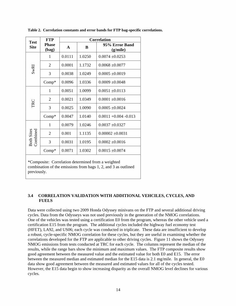
Table 2 shows the constants for the bag-specific correlations, including both site-specific correlations as well as a correlation using the data from both SwRI and TRC. The constants are used in the same way as discussed above for the composite estimate. The error band containing at least 95% of the results is also presented.

14

Table 2. Correlation constants and error bands for FTP bag-specific correlations.

Test Site

FTP Phase (bag)

Correlation

A B 95% Error Band

(g/mile)

Sw

RI

1 0.0111 1.0250 0.0074 ±0.0253

2 0.0001 1.1732 0.0068 ±0.0077

3 0.0038 1.0249 0.0005 ±0.0019

Comp* 0.0096 1.0336 0.0009 ±0.0048

TR

C

1 0.0051 1.0099 0.0051 ±0.0113

2 0.0021 1.0349 0.0001 ±0.0016

3 0.0025 1.0090 0.0005 ±0.0024

Comp* 0.0047 1.0140 0.0011 +0.004 -0.013

Bot

h S

ites

C

ombi

ned

1 0.0079 1.0246 0.0037 ±0.0327

2 0.001 1.1135 0.00002 ±0.0031

3 0.0031 1.0195 0.0002 ±0.0016

Comp* 0.0071 1.0302 0.0015 ±0.0074

*Composite: Correlation determined from a weighted combination of the emissions from bags 1, 2, and 3 as outlined previously.

3.4 CORRELATION VALIDATION WITH ADDITIONAL VEHCILES, CYCLES, AND FUELS

Data were collected using two 2009 Honda Odyssey minivans on the FTP and several additional driving cycles. Data from the Odysseys was not used previously in the generation of the NMOG correlations. One of the vehicles was tested using a certification E0 from the program, whereas the other vehicle used a certification E15 from the program. The additional cycles included the highway fuel economy test (HFET), LA92, and US06; each cycle was conducted in triplicate. These data are insufficient to develop a robust, cycle-specific NMOG correlation for these cycles, but they are useful in examining whether the correlations developed for the FTP are applicable to other driving cycles. Figure 11 shows the Odyssey NMOG emissions from tests conducted at TRC for each cycle. The columns represent the median of the results, while the range bars show the minimum and maximum values. The FTP composite results show good agreement between the measured value and the estimated value for both E0 and E15. The error between the measured median and estimated median for the E15 data is 2.1 mg/mile. In general, the E0 data show good agreement between the measured and estimated values for all of the cycles tested. However, the E15 data begin to show increasing disparity as the overall NMOG level declines for various cycles.

15

Interestingly, the range bars for the estimate tend to show lower ranges in the estimated NMOG emissions compared to the ranges of the measured NMOG emissions. Since the NMOG estimate is a scalar multiplier of the measured NMHC emissions level, this trend indicates that the OHC measurements, rather than the NMHC measurements, have increasing variability as the overall NMOG level declines. This issue is especially evident in the very low NMOG emissions for the HFET cycle. The root cause of this variability is unknown but might arise from either actual variation in the emissions levels of NMOG compounds from the vehicles or from measurement uncertainties imposed from characterization of emissions at such low levels. Since both the HFET and US06 are executed when the vehicle has a hot catalyst and there is no engine start that can add variability to the emissions, it seems likely that measurement error associated with speciation of the individual NMOG species is a significant component of the NMOG emissions variability. It is encouraging, however, that the NMOG emissions for two vehicles that were not a part of the development of the estimation technique can be estimated with reasonable accuracy both on the FTP as well as other common cycles.

Figure 11. Measured and estimated NMOG emissions for additional cycles. Columns represent the median result; range bars show the maximum and minimum results.

Several FTP tests were also conducted at TRC using a retail (pump) E0 and an E20 splash blended from the same retail E0 fuel. The data from these tests were not used in producing the NMOG correlations but are useful to assess whether the correlations are valid for fuels that were not originally used in the study. Two vehicles tested previously during the program were used for these tests: a 2005 Toyota Tundra and a 2009 Honda Civic. Duplicate tests using both E0 and E20 were conducted with both vehicles. Figure 12 shows the estimated and measured composite NMOG emissions. E0 data are shown as black points, with E20 data in red. The E0 data are generally of lower error level than the E20 data as shown by the 1:1 line in the figure. The average error level for the E0 tests was -0.97 mg/mile and was -2.38 mg/mile for the E20 tests. In all eight tests, the estimate was higher than the measured value; this outcome is likely due to the use of the correlation developed using data from both TRC and SwRI. Using the correlation developed with only the TRC data reduces these errors to -0.36 mg/mile for the E0 data and -1.29

0

5

10

15

20

25

30

35

40

45

50

55

60

FTP LA92 US06 HFET

NM

OG

Emis

sion

s (m

g/m

ile)

E0 Measured

E0 Estimated

E15 Measured

E15 Estimated

16

mg/mile for the E20 results. These error levels are consistent with the overall error levels from the program data, indicating that the correlations appear to hold for these non-certification ethanol-blended fuels.

Figure 12. Comparison of estimated and measured FTP composite NMOG emissions for two vehicles using non-certification fuels.

3.5 NMOG MEASUREMENT CONSIDERATIONS

It is important to note that the emissions tests conducted during this study were conducted per the EPA regulations for gasoline-fueled vehicles, not those for flex-fuel vehicles. One aspect of these regulations that may have an impact on the NMOG emissions measurements is that a temperature-controlled exhaust transfer line from the vehicle to the dilution tunnel is not required, and was not used for these tests. Such a transfer line is specified for use when flex-fuel vehicle tests are conducted. The boiling point of acetaldehyde is 21 °C and thus it is not likely that significant loss of acetaldehyde (or formaldehyde, since it boils at a lower temperature) will occur in the transfer line at ambient test cell conditions. However, the boiling point of ethanol is 79 °C, and so it is possible that small amounts of ethanol are lost due to condensation on the transfer line walls during the cold-start portion of the FTP. Since most of the emissions in bag 1 occur during the initial moments of the cycle, it is possible, and perhaps likely, that ethanol adhering to the transfer line surfaces will re-vaporize and be correctly measured as a part of the bag 1 emissions. However, some of the ethanol may remain and be measured as carryover into bag 2 or be lost entirely. While this phenomenon would likely not be a problem at relatively high emissions levels, it may become more significant as regulatory emissions levels decrease. Similarly, small sections of unheated tubing leading from the dilution tunnel system into the impingers used to trap the ethanol in the gas sample may also be a source for error due to condensation or physisorption. If ethanol is

17

introduced in certification fuel, it may be useful to consider new designs for the impinger apparatus to avoid potential ethanol loss or carryover.

Another potential concern is error associated with the measurement of such small quantities of individual OHC species. Measurements of ethanol at substantially less than 1 mg/mile accuracy require exceptionally high fidelity gas chromatography methods. One path towards improvement is through re-design of the impinger itself in order to enable higher sample flow rates without substantially increasing the liquid volume in the impinger. Raising the sample flow rate while holding the liquid volume constant can enable increases in analyte concentration in the impinger liquid, thus improving the analytical accuracy for even very low vehicle emissions levels.

Similar measurement concerns exist for the DNPH analysis of carbonyl species. A study conducted in Japan found that chilling the cartridges during sampling can help with trapping efficiency [8]. Additionally, since acetone is included as a measured NMOG species and is ubiquitous in most analytical chemistry laboratories as a solvent, contamination of the DNPH cartridge during handling and analysis may become a concern. One study has identified O-(4-cyano-2-methoxybenzyl) hydroxyl amine (CNET) as an alternative reagent that has the potential to improve both the trapping and background issues associated with DNPH sampling. This method seems to show promise, but the CNET was found to produce formaldehyde and acetaldehyde in the presence of high levels of NOX [8,9]. The authors of the CNET study also highlight the potential for acetone contamination during sample handling. Given the overall dominance of ethanol, formaldehyde, and acetaldehyde in the fractionation of the vehicle OHC emissions, the most straightforward solution to potential acetone contamination may be to neglect acetone emissions in the calculation of NMOG emissions.

18

4. CONCLUSIONS

• The NMOG/NMHC ratio that is characteristic of emissions from ethanol-blended fuels is a function of the ethanol blend level in the fuel; the NMOG/NMHC ratio for ethanol-blended fuels is in excess of the 1.04 factor previously allowed by EPA for estimation of NMOG emissions for ethanol-free certification gasoline.

• A method has been developed based on a large body of data from two test laboratories to estimate NMOG emissions on the FTP cycle when fuels containing ethanol are used. The method has been shown to estimate the composite NMOG emissions with an error of 0.0015 ±0.0074 g/mile.

• The correlation developed for estimating FTP composite NMOG emissions also provides a reasonably accurate estimate for the LA92, US06, and HFET cycles for the two vehicles that were tested using these cycles.

• Increased error relative to the measured NMOG emissions values is evident at NMOG levels below 0.010 g/mile, though the error remains comparable to higher emissions cases when examined in an absolute sense. Such low NMOG emissions levels may be achieved on the FTP in bags 2 and 3, or during other cycles such as the HFET.

• NMOG emissions estimates for eight FTP tests that were conducted using two retail fuels that were not a part of the correlation development agreed reasonably well with measured values, indicating that the correlations are valid for other ethanol-blended fuels.

• The level of error in the measurement at NMOG levels below 0.010 g/mile may be substantially influenced by measurement limitations associated with current practices in sample capture and analysis using impingers and DNPH cartridges.

5. REFERENCES

1. “Partial Grant and Partial Denial of Clean Air Act Waiver Application to Increase the Allowable

Ethanol Content of Gasoline to 15 Percent; Decision of the Administrator,” Federal Register Vol. 75, Issue 213, November 4, 2010.

2. “Partial Grant of Clean Air Act Waiver Application Submitted by Growth Energy to Increase the Allowable Ethanol Content of Gasoline to 15 Percent; Decision of the Administrator,” Federal Register Vol. 76, Issue 17, January 26, 2011.

3. Code of Federal Regulations, Title 40, Part 86, subpart S, section 86.1810-01, issued July 2010. 4. Code of Federal Regulations, Title 40, Part 86, subpart B, section 86.144-94, issued July 2010. 5. Brian H. West, C. Scott Sluder, Keith E. Knoll, John E. Orban, “Intermediate Ethanol Blends Catalyst

Durability Program,” report ORNL/TM-2011/234, Oak Ridge National Laboratory, Oak Ridge, Tennessee, September 2011.

6. “Control of Hazardous Air Pollutants from Mobile Sources,” Federal Register Vol. 72, Issue 37, February 26, 2007.

7. Kenneth Kar and Wai K. Cheng, “Speciated Engine-Out Organic Gas Emissions from a PFI-SI Engine Operating on Ethanol/Gasoline Mixtures,” SAE Technical Paper 2009-01-2673, 2009.

8. Kenichi Akiyama and Akemi Nakayama, “Study on Reliable Automotive Exhaust Acrolein Collection Method,” SAE Technical Paper 2010-01-2207, 2010.

9. Ken-ichi Akiyama and Akemi Nakayama, “Analysis of Low Concentration Aldehyde and Ketone Compounds in Automotive Exhaust Gas by New Collection Reagent,” SAE Technical Paper 2005-01-2152, 2005.