Nick Wintermantel | Principal, Astrapé Consulting, LLC
164
Nick Wintermantel | Principal, Astrapé Consulting, LLC 3000 Riverchase Galleria Hoover, AL 35224 (205) 988-4404 nwintermantel@Astrapé.com Mr. Wintermantel has 20 years of experience in utility planning and electric market modeling. Areas of utility planning experience includes utility integrated resource planning (IRP) for vertically-integrated utilities, market price forecasting, resource adequacy modeling, RFP evaluations, environmental compliance analysis, asset management, financial risk analysis, and contract structuring. Mr. Wintermantel also has expertise in production cost simulations and evaluation methodologies used for IRPs and reliability planning. As a consultant with Astrapé Consulting, Mr. Wintermantel has managed reliability and planning studies for large power systems across the U.S. and internationally. Prior to joining Astrapé Consulting, Mr. Wintermantel was employed by the Southern Company where he served in various resource planning, asset management, and generation development roles. Experience Principal Consultant at Astrapé Consulting (2009 – Present) Managed detailed system resource adequacy studies for large scale utilities Managed ancillary service and renewable integration studies Managed capacity value studies Managed resource selection studies Performed financial and risk analysis for utilities, developers, and manufacturers Demand side resource evaluation Storage evaluation Served on IE Teams to evaluate assumptions, models, and methodologies for competitive procurement solicitations Project Management on large scale consulting engagements Production cost model development Model quality assurance Sales and customer service Sr. Engineer for Southern Company Services (2007-2009) Integrated Resource Planning and environmental compliance Developed future retail projects for operating companies while at the Southern Company Asset management for Southern Company Services Sr. Engineer for Southern Power Company (Subsidiary of Southern Company) (2003-2007) Structured wholesale power contracts for Combined Cycle, Coal, Simple Cycle, and IGCC Projects Model development to forecast market prices across the eastern interconnect Evaluate financials of new generation projects Bid development for Resource Solicitations Cooperative Student Engineer for Southern Nuclear (2000-2003) Probabilistic risk assessment of the Southern Company Nuclear Fleet Wintermantel DEC.DEP Exhibit 1 Docket Nos. 2019-224-E & 2019-225-E ELECTRONICALLY FILED - 2020 November 13 4:46 PM - SCPSC - Docket # 2019-225-E - Page 1 of 164
Transcript of Nick Wintermantel | Principal, Astrapé Consulting, LLC

Nick Wintermantel | Principal, Astrapé Consulting, LLC
3000 Riverchase Galleria Hoover, AL 35224 (205) 988-4404nwintermantel@Astrapé.com
Mr. Wintermantel has 20 years of experience in utility planning and electric market modeling. Areas of utility planning experience includes utility integrated resource planning (IRP) for vertically-integrated utilities, market price forecasting, resource adequacy modeling, RFP evaluations, environmental compliance analysis, asset management, financial risk analysis, and contract structuring. Mr. Wintermantel also has expertise in production cost simulations and evaluation methodologies used for IRPs and reliability planning. As a consultant with Astrapé Consulting, Mr. Wintermantel has managed reliability and planning studies for large power systems across the U.S. and internationally. Prior to joining Astrapé Consulting, Mr. Wintermantel was employed by the Southern Company where he served in various resource planning, asset management, and generation development roles.
Experience
Principal Consultant at Astrapé Consulting (2009 – Present) Managed detailed system resource adequacy studies for large scale utilities Managed ancillary service and renewable integration studies Managed capacity value studies Managed resource selection studies Performed financial and risk analysis for utilities, developers, and manufacturers Demand side resource evaluation Storage evaluation Served on IE Teams to evaluate assumptions, models, and methodologies for competitive procurement solicitations Project Management on large scale consulting engagements Production cost model development Model quality assurance Sales and customer service
Sr. Engineer for Southern Company Services (2007-2009) Integrated Resource Planning and environmental compliance Developed future retail projects for operating companies while at the Southern Company Asset management for Southern Company Services
Sr. Engineer for Southern Power Company (Subsidiary of Southern Company) (2003-2007) Structured wholesale power contracts for Combined Cycle, Coal, Simple Cycle, and IGCC Projects Model development to forecast market prices across the eastern interconnect Evaluate financials of new generation projects Bid development for Resource Solicitations
Cooperative Student Engineer for Southern Nuclear (2000-2003) Probabilistic risk assessment of the Southern Company Nuclear Fleet
Wintermantel DEC.DEP Exhibit 1 Docket Nos. 2019-224-E & 2019-225-E
ELECTR
ONICALLY
FILED-2020
Novem
ber134:46
PM-SC
PSC-D
ocket#2019-225-E
-Page1of164

2
Industry Specialization
Resource Adequacy Planning
Competitive Procurement
Environmental Compliance Analysis
Renewable Integration
Resource Planning
Asset Evaluation
Generation Development
Ancillary Service Studies
Integrated Resource Planning
Financial Analysis
Capacity Value Analysis
Education
MBA, University of Alabama at Birmingham – Summa Cum Laude B.S. Degree Mechanical Engineering - University of Alabama - Summa Cum Laude
Relevant Experience
Resource Adequacy Planning and Production Cost Modeling
Tennessee Valley Authority: Performed Various Reliability Planning Studies including Optimal Reserve Margin Analysis, Capacity Benefit Margin Analysis, and Demand Side Resource Evaluations using the Strategic Energy and Risk Valuation Model (SERVM) which is Astrapé Consulting’s proprietary reliability planning software. Recommended a new planning target reserve margin for the TVA system and assisted in structuring new demand side option programs in 2010. Performed Production Cost and Resource Adequacy Studies in 2009, 2011, 2013, 2015 and 2017. Performed renewable integration and ancillary service work from 2015-2017.
Southern Company Services: Assisted in resource adequacy and capacity value studies as well as model development from 2009 – 2018.
Louisville Gas & Electric and Kentucky Utilities: Performed reliability studies including reserve margin analysis for its Integrated Resource Planning process. Ongoing support for Resource Adequacy from 2011 – 2020.
Duke Energy: Performed resource adequacy studies for Duke Energy Carolinas, LLC and Duke Energy Progress, LLC in 2012 and 2016. Performed capacity value and ancillary service studies in 2018. Performed Resource Adequacy and Battery ELCC Study in 2020.
California Energy Systems for the 21st Century Project: Performed 2016 Flexibility Metrics and Standards Project. Developed new flexibility metrics such as EUEflex and LOLEflex which represent LOLE occurring due to system flexibility constraints and not capacity constraints.
Terna: Performed Resource Adequacy Study used to set demand curves in Italian Capacity Market Design.
Pacific Gas and Electric (PG&E): Performed flexibility requirement and ancillary service study from 2015–2017. Performed CES Study for Renewable Integration and Flexibility from 2015 – 2016.
PNM (Public Service Company of New Mexico): Managed resource adequacy studies, renewable integration studies and ancillary service studies from 2013 – 2020. Performed resource selection studies in 2017 and 2018. Evaluated storage.
GASOC: Managed resource adequacy studies from 2015 – 2018.
Wintermantel DEC.DEP Exhibit 1 Docket Nos. 2019-224-E & 2019-225-E
ELECTR
ONICALLY
FILED-2020
Novem
ber134:46
PM-SC
PSC-D
ocket#2019-225-E
-Page2of164
AgTRAPE CONSULTINGinno enon n electric ty tent pl nn ng

3
MISO: Managed resource adequacy study and provided support from 2015 – 2020.
SPP: Managed resource adequacy study in 2017 and provided ongoing support through 2020. Performed a Storage ELCC Study in 2019.
Malaysia (TNB, Sabah, Sarawak)): Performed and managed resource adequacy studies from 2015-2018 for three different Malaysian entities.
ERCOT: Performed economic optimal reserve margin studies in cooperation with the Brattle Group in 2014 and 2018. The report examined total system costs, generator energy margins, reliability metrics, and economics under various market structures (energy only vs. capacity markets). Completed a Reserve Margin Study requested by the PUCT, examining an array of physical reliability metrics in 2014 (See Publications: Expected Unserved Energy and Reserve Margin Implications of Various Reliability Standards). Probabilistic Risk Assessment for the North American Electric Reliability Corporation (NERC) in 2014, 2016, and 2018.
FERC: Performed economics of resource adequacy work in 2012-2013 in cooperation with the Brattle Group. Work included analyzing resource adequacy from regulated utility and structured market perspective.
EPRI: Performed research projects studying reliability impact and flexibility requirements needed with increased penetration of intermittent resources in 2013. Created Risk-Based Planning system reliability metrics framework in 2014 that is still in use today.
California Public Utilities Commission: Provided ongoing support for Resource Adequacy work.
Wintermantel DEC.DEP Exhibit 1 Docket Nos. 2019-224-E & 2019-225-E
ELECTR
ONICALLY
FILED-2020
Novem
ber134:46
PM-SC
PSC-D
ocket#2019-225-E
-Page3of164
AgTRAPE CONSULTINGinno enon n electric ty tent pl nn ng

Duke Energy Carolinas
2020 Resource Adequacy Study
9/1/2020
PREPARED FOR
Duke Energy
PREPARED BY
Kevin Carden Nick Wintermantel Cole Benson Astrapé Consulting
Wintermantel DEC Exhibit 2ELEC
TRONICALLY
FILED-2020
Novem
ber134:46
PM-SC
PSC-D
ocket#2019-225-E
-Page4of164
A TRAPE CONS ULTINGinnovation in electric system planning

DEC 2020 Resource Adequacy Study
1
ContentsExecutive Summary ...................................................................................................................................... 3
I. List of Figures ......................................................................................................................................... 19
II. List of Tables .......................................................................................................................................... 20
III. Input Assumptions ................................................................................................................................ 21
A. Study Year ...................................................................................................................................... 21
B. Study Topology ............................................................................................................................... 21
C. Load Modeling ................................................................................................................................ 22
D. Economic Load Forecast Error ....................................................................................................... 27
E. Conventional Thermal Resources ................................................................................................... 29
F. Unit Outage Data ............................................................................................................................ 30
G. Solar and Battery Modeling ............................................................................................................ 33
H. Hydro Modeling .............................................................................................................................. 35
I. Demand Response Modeling .......................................................................................................... 37
J. Operating Reserve Requirements .................................................................................................... 38
K. External Assistance Modeling ........................................................................................................ 38
L. Cost of Unserved Energy ................................................................................................................ 40
M. System Capacity Carrying Costs .................................................................................................... 41
IV. Simulation Methodology ...................................................................................................................... 42
A. Case Probabilities ............................................................................................................................ 42
B. Reserve Margin Definition.............................................................................................................. 44
V. Physical Reliability Results.................................................................................................................... 45
VI. Base Case Economic Results ................................................................................................................ 49
VII. Sensitivities ......................................................................................................................................... 54
Outage Sensitivities ................................................................................................................................ 54
Load Forecast Error Sensitivities ............................................................................................................ 55
Solar Sensitivities.................................................................................................................................... 56
Demand Response (DR) Sensitivity ....................................................................................................... 57
No Coal Sensitivity ................................................................................................................................. 58
Climate Change Sensitivity ..................................................................................................................... 59
VIII. Economic Sensitivities ....................................................................................................................... 60
IX. DEC/DEP Combined Sensitivity .......................................................................................................... 61
X. Conclusions ............................................................................................................................................ 62
Wintermantel DEC Exhibit 2ELEC
TRONICALLY
FILED-2020
Novem
ber134:46
PM-SC
PSC-D
ocket#2019-225-E
-Page5of164

DEC 2020 Resource Adequacy Study
2
XI. Appendix A ........................................................................................................................................... 64
XII. Appendix B.......................................................................................................................................... 65
Wintermantel DEC Exhibit 2ELEC
TRONICALLY
FILED-2020
Novem
ber134:46
PM-SC
PSC-D
ocket#2019-225-E
-Page6of164

DEC 2020 Resource Adequacy Study
3
Executive Summary
This study was performed by Astrapé Consulting at the request of Duke Energy Carolinas (DEC)
as an update to the study performed in 2016. The primary purpose of this study is to provide Duke
system planners with information on physical reliability and costs that could be expected with
various reserve margin1 planning targets. Physical reliability refers to the frequency of firm load
shed events and is calculated using Loss of Load Expectation (LOLE). The one day in 10-year
standard (LOLE of 0.1) is interpreted as one day with one or more hours of firm load shed every
10 years due to a shortage of generating capacity and is used across the industry2 to set minimum
target reserve margin levels. Astrapé determined the reserve margin required to meet the one day
in 10-year standard for the Base Case and multiple sensitivities included in the study. The study
includes a Confidential Appendix containing confidential information such as fuel costs, outage
rate data and transmission assumptions.
Customers expect to have electricity during all times of the year but especially during extreme
weather conditions such as cold winter days when resource adequacy3 is at risk for DEC4. In order
1 Throughout this report, winter and summer reserve margins are defined by the formula: (installed capacity - peak load) / peak load. Installed capacity includes capacity value for intermittent resources such as solar and energy limited resources such as battery. 2 https://www.ferc.gov/sites/default/files/2020-05/02-07-14-consultant-report.pdf; See Table 14 in A-1. PJM, MISO, NYISO ISO-NE, Quebec, IESO, FRCC, APS, NV Energy all use the 1 day in 10 year standard. As of this report, it is Astrapé’s understanding that Southern Company has shifted to the greater of the economic reserve margin or the 1 day in 10 year standard. 3 NERC RAPA Definition of “Adequacy” - The ability of the electric system to supply the aggregate electric power and energy requirements of the electricity consumers at all times, taking into account scheduled and expected unscheduled outages of system components. https://www.nerc.com/pa/RAPA/ra/Reliability%20Assessments%20DL/NERC_LTRA_2019.pdf, at 9. 4 Section (b)(4)(iv) of NCUC Rule R8-61 (Certificate of Public Convenience and Necessity for Construction of Electric Generation Facilities) requires the utility to provide “… a verified statement as to whether the facility will be capable of operating during the lowest temperature that has been recorded in the area using information from the National Weather Service Automated Surface Observing System (ASOS) First Order Station in Asheville, Charlotte, Greensboro, Hatteras, Raleigh or Wilmington, depending upon the station that is located closest to where the plant will be located.”
Wintermantel DEC Exhibit 2ELEC
TRONICALLY
FILED-2020
Novem
ber134:46
PM-SC
PSC-D
ocket#2019-225-E
-Page7of164

DEC 2020 Resource Adequacy Study
4
to ensure reliability during these peak periods, DEC maintains a minimum reserve margin level to
manage unexpected conditions including extreme weather, load growth, and significant forced
outages. To understand this risk, a wide distribution of possible scenarios must be simulated at a
range of reserve margins. To calculate physical reliability and customer costs for the DEC system,
Astrapé Consulting utilized a reliability model called SERVM (Strategic Energy and Risk
Valuation Model) to perform thousands of hourly simulations for the 2024 study year at various
reserve margin levels. Each of the yearly simulations was developed through a combination of
deterministic and stochastic modeling of the uncertainty of weather, economic growth, unit
availability, and neighbor assistance.
In the 2016 study, reliability risk was concentrated in the winter and the study determined that a
16.5% reserve margin was required to meet the one day in 10-year standard (LOLE of 0.1), for
DEC. Because DEC’s sister utility DEP required a 17.5% reserve margin to meet the same
reliability standard, Duke Energy averaged the studies and used a 17% planning reserve margin
target for both companies in its Integrated Resource Plan (IRP). This 2020 Study updates all input
assumptions to reassess resource adequacy. As part of the update, several stakeholder meetings
occurred to discuss inputs, methodology, and results. These stakeholder meetings included
representatives from the North Carolina Public Staff, the South Carolina Office of Regulatory Staff
(ORS), and the North Carolina Attorney General’s Office. Following the initial meeting with
stakeholders on February 21, 2020, the parties agreed to the key assumptions and sensitivities
listed in Appendix A, Table A.1.
Wintermantel DEC Exhibit 2ELEC
TRONICALLY
FILED-2020
Novem
ber134:46
PM-SC
PSC-D
ocket#2019-225-E
-Page8of164

DEC 2020 Resource Adequacy Study
5
Preliminary results were presented to the stakeholders on May 8, 2020 and additional follow up
was done throughout the month of May. Moving from the 2016 Study, the Study Year was shifted
from 2019 to 2024 and assumed solar capacity was updated to the most recent projections.
Because solar projections increased, LOLE has continued to shift from the summer to the winter.
The high volatility in peak winter loads seen in the 2016 Study remained evident in recent historical
data. In response to stakeholder feedback, the four year ahead economic load forecast error was
dampened by providing a higher probability weighting on over-forecasting scenarios relative to
under-forecasting scenarios. The net effect of the new distribution is to slightly reduce the target
reserve margin compared to the previous distribution supplying slight upward pressure on the
target reserve margin. This means that if the target reserve margin from this study is adopted, no
reserves would be held for potential under-forecast of load growth. Generator outages remained
in line with 2016 expectations, but additional cold weather outages of 260 MW for DEC were
included for temperatures less than 10 degrees.
Physical Reliability Results-Island
Table ES1 shows the monthly contribution of LOLE at various reserve margin levels for the Island
scenario. In this scenario, it is assumed that DEC is responsible for its own load and that there is
no assistance from neighboring utilities. The summer and winter reserve margins differ for all
scenarios due to seasonal demand forecast differences, weather-related thermal generation
capacity differences, demand response seasonal availability, and seasonal solar capacity value.
Using the one day in 10-year standard (LOLE of 0.1), which is used across the industry to set
minimum target reserve margin levels, DEC would require a 22.5% winter reserve margin in the
Island Case where no assistance from neighboring systems was assumed.
Wintermantel DEC Exhibit 2ELEC
TRONICALLY
FILED-2020
Novem
ber134:46
PM-SC
PSC-D
ocket#2019-225-E
-Page9of164

DEC 2020 Resource Adequacy Study
6
Given the significant level of solar on the system, the summer reserves are approximately 2%
greater than winter reserves which results in essentially no reliability risk in the summer months
when total LOLE is 0.1 days per year. This 22.5% reserve margin is required to cover the
combined risks seen in load uncertainty, weather uncertainty, and generator performance for the
DEC system. As discussed below, when compared to Base Case results which recognizes neighbor
assistance, results of the Island Case illustrate both the benefits and risks of carrying lower reserve
margins through reliance on neighboring systems.
Table ES1. Island Physical Reliability Results
Winter Reserve Margin
Summer Reserve Margin
Jan Feb Mar Apr May Jun Jul Aug Sep Oct Nov Dec Summer LOLE
Winter LOLE
Total LOLE
10.0% 12.4% 0.81 0.14 0.08 - 0.00 0.12 0.70 0.80 0.31 0.11 0.02 0.27 2.05 1.31 3.36
11.0% 13.3% 0.69 0.12 0.06 - 0.00 0.09 0.48 0.51 0.19 0.07 0.01 0.20 1.35 1.09 2.44
12.0% 14.2% 0.58 0.10 0.05 - 0.00 0.06 0.31 0.33 0.12 0.04 0.01 0.15 0.87 0.88 1.75
13.0% 15.0% 0.48 0.08 0.04 - 0.00 0.04 0.19 0.21 0.07 0.03 0.00 0.11 0.55 0.71 1.26
14.0% 15.9% 0.40 0.07 0.03 - 0.00 0.02 0.11 0.14 0.04 0.02 0.00 0.08 0.34 0.58 0.92
15.0% 16.8% 0.33 0.06 0.03 - - 0.02 0.07 0.09 0.03 0.01 - 0.06 0.21 0.47 0.68
16.0% 17.6% 0.28 0.05 0.02 - - 0.01 0.04 0.05 0.02 0.01 - 0.04 0.13 0.39 0.52
17.0% 18.5% 0.23 0.04 0.02 - - 0.01 0.03 0.03 0.01 0.00 - 0.03 0.09 0.32 0.41
18.0% 19.4% 0.19 0.03 0.01 - - 0.01 0.02 0.02 0.01 0.00 - 0.03 0.06 0.27 0.33
19.0% 20.2% 0.16 0.03 0.01 - - 0.01 0.02 0.01 0.00 - - 0.02 0.04 0.22 0.26
20.0% 21.1% 0.13 0.02 0.01 - - 0.00 0.01 0.01 0.00 - - 0.02 0.02 0.18 0.20
21.0% 22.0% 0.11 0.02 0.00 - - 0.00 0.00 0.01 0.00 - - 0.01 0.01 0.14 0.15
22.0% 22.8% 0.08 0.01 0.00 - - 0.00 0.00 0.01 0.00 - - 0.01 0.01 0.10 0.11
23.0% 23.7% 0.06 0.01 0.00 - - 0.00 0.00 0.00 0.00 - - 0.00 0.00 0.08 0.08
24.0% 24.6% 0.05 0.01 0.00 - - 0.00 0.00 0.00 0.00 - - 0.00 0.00 0.06 0.06
Wintermantel DEC Exhibit 2ELEC
TRONICALLY
FILED-2020
Novem
ber134:46
PM-SC
PSC-D
ocket#2019-225-E
-Page10
of164

DEC 2020 Resource Adequacy Study
7
Physical Reliability Results-Base Case
Astrapé recognizes that DEC is part of the larger eastern interconnection and models neighbors
one tie away to allow for market assistance during peak load periods. However, it is important to
also understand that there is risk in relying on neighboring capacity that is less dependable than
owned or contracted generation in which DEC would have first call rights. While there are
certainly advantages of being interconnected due to weather diversity and generator outage
diversity across regions, market assistance is not guaranteed and Astrapé believes Duke Energy
has taken a moderate to aggressive approach (i.e. taking significant credit for neighboring regions)
to modeling neighboring assistance compared to other surrounding entities such as PJM
Interconnection L.L.C. (PJM)5 and the Midcontinent Independent System Operator (MISO)6. A
full description of the market assistance modeling and topology is available in the body of the
report. Table ES2 shows the monthly LOLE at various reserve margin levels for the Base Case
scenario which is the Island scenario with neighbor assistance included.7
5 PJM limits market assistance to 3,500 MW which represents approximately 2.3% of its reserve margin compared to 6.5% assumed for DEC. https://www.pjm.com/-/media/committees-groups/subcommittees/raas/20191008/20191008-pjm-reserve-requirement-study-draft-2019.ashx – page 11 6MISO limits external assistance to a Unforced Capacity (UCAP) of 2,331 MW which represents approximately 1.8% of its reserve margin compared to 6.5% assumed for DEC. https://www.misoenergy.org/api/documents/getbymediaid/80578 page 24 (copy and paste link in browser) 7 Reference Appendix B, Table B.1 for percentage of loss of load by month and hour of day for the Base Case.
Wintermantel DEC Exhibit 2ELEC
TRONICALLY
FILED-2020
Novem
ber134:46
PM-SC
PSC-D
ocket#2019-225-E
-Page11
of164

DEC 2020 Resource Adequacy Study
8
Table ES2. Base Case Physical Reliability Results
Winter Reserve Margin
Summer Reserve Margin
Jan Feb Mar Apr May Jun Jul Aug Sep Oct Nov Dec Summer LOLE
Winter LOLE
Total LOLE
5.00% 8.11% 0.21 0.05 0.02 0.00 0.00 0.00 0.02 0.02 0.00 0.00 0.00 0.04 0.05 0.33 0.38
6.00% 8.97% 0.20 0.05 0.02 0.00 0.00 0.00 0.02 0.02 0.00 0.00 0.00 0.04 0.04 0.30 0.35
7.00% 9.84% 0.18 0.05 0.02 0.00 0.00 0.00 0.02 0.01 0.00 0.00 0.00 0.03 0.04 0.28 0.31
8.00% 10.71% 0.17 0.04 0.01 0.00 0.00 0.00 0.02 0.01 0.00 0.00 0.00 0.03 0.03 0.25 0.28
9.00% 11.57% 0.15 0.04 0.01 0.00 0.00 0.00 0.01 0.01 0.00 0.00 0.00 0.03 0.03 0.23 0.25
10.00% 12.44% 0.14 0.04 0.01 0.00 0.00 0.00 0.01 0.01 0.00 0.00 0.00 0.02 0.02 0.21 0.23
11.00% 13.31% 0.13 0.03 0.01 0.00 0.00 0.00 0.01 0.01 0.00 0.00 0.00 0.02 0.02 0.18 0.20
12.00% 14.18% 0.11 0.03 0.01 0.00 0.00 0.00 0.01 0.01 0.00 0.00 0.00 0.01 0.01 0.16 0.18
13.00% 15.04% 0.10 0.03 0.00 0.00 0.00 0.00 0.00 0.00 0.00 0.00 0.00 0.01 0.01 0.15 0.15
14.00% 15.91% 0.09 0.02 0.00 0.00 0.00 0.00 0.00 0.00 0.00 0.00 0.00 0.01 0.01 0.13 0.13
15.00% 16.78% 0.08 0.02 0.00 0.00 0.00 0.00 0.00 0.00 0.00 0.00 0.00 0.01 0.00 0.11 0.12
16.00% 17.64% 0.07 0.02 0.00 0.00 0.00 0.00 0.00 0.00 0.00 0.00 0.00 0.01 0.00 0.10 0.10
17.00% 18.51% 0.06 0.02 0.00 0.00 0.00 0.00 0.00 0.00 0.00 0.00 0.00 0.00 0.00 0.08 0.08
18.00% 19.38% 0.05 0.01 0.00 0.00 0.00 0.00 0.00 0.00 0.00 0.00 0.00 0.00 0.00 0.07 0.07
19.00% 20.24% 0.05 0.01 0.00 0.00 0.00 0.00 0.00 0.00 0.00 0.00 0.00 0.00 0.00 0.06 0.06
20.00% 21.11% 0.04 0.01 0.00 0.00 0.00 0.00 0.00 0.00 0.00 0.00 0.00 0.00 0.00 0.05 0.05
21.00% 21.98% 0.03 0.01 0.00 0.00 0.00 0.00 0.00 0.00 0.00 0.00 0.00 0.00 0.00 0.04 0.04
22.00% 22.84% 0.03 0.00 0.00 0.00 0.00 0.00 0.00 0.00 0.00 0.00 0.00 0.00 0.00- 0.03 0.03
As the table indicates, the required reserve margin to meet the one day in 10-year standard (LOLE
of 0.1), is 16.00% which is 6.50% lower than the required reserve margin for 0.1 LOLE in the
Island scenario. Approximately one third of the 22.5% required reserves is reduced due to
interconnection ties. Astrapé also notes utilities around the country are continuing to retire and
replace fossil-fuel resources with more intermittent or energy limited resources such as solar, wind,
and battery capacity. For example, Dominion Energy Virginia has made substantial changes to its
plans as this study was being conducted and plans to add substantial solar and other renewables to
Wintermantel DEC Exhibit 2ELEC
TRONICALLY
FILED-2020
Novem
ber134:46
PM-SC
PSC-D
ocket#2019-225-E
-Page12
of164

DEC 2020 Resource Adequacy Study
9
its system that could cause additional winter reliability stress than what is modeled. The below
excerpt is from page 6 of Dominion Energy Virginia’s 2020 IRP8:
In the long term, based on current technology, other challenges will arise from the significant development of intermittent solar resources in all Alternative Plans. For example, based on the nature of solar resources, the Company will have excess capacity in the summer, but not enough capacity in the winter. Based on current technology, the Company would need to meet this winter deficit by either building additional energy storage resources or by buying capacity from the market. In addition, the Company would likely need to import a significant amount of energy during the winter, but would need to export or store significant amounts of energy during the spring and fall.
Additionally, PJM now considers the DOM Zone to be a winter peaking zone where winter peaks
are projected to exceed summer peaks for the forecast period.9 While this is only one example,
these potential changes to surrounding resource mixes may lead to less confidence in market
assistance for the future during early morning winter peak loads. Changes in neighboring system
resource portfolios and load profiles will be an important consideration in future resource adequacy
studies. To the extent historic diversification between DEC and neighboring systems declines, the
historic reliability benefits DEC has experienced from being an interconnected system will also
decline. It is worth nothing that after this study was completed, California experienced rolling
blackouts during extreme weather conditions as the ability to rely on imported power has declined
and has shifted away from dispatchable fossil-fuel resources and put greater reliance on
intermittent resources.10 It is premature to fully ascertain the lessons learned from the California
load shed events. However, it does highlight the fact that as DEC reduces dependence on
8 https://cdn-dominionenergy-prd-001.azureedge.net/-/media/pdfs/global/2020-va-integrated-resource-plan.pdf?la=en&rev=fca793dd8eae4ebea4ee42f5642c9509 9 Dominion Energy Virginia 2020 IRP, at 40. 10 http://www.caiso.com/Documents/ISO-Stage-3-Emergency-Declaration-Lifted-Power-Restored-Statewide.pdf
Wintermantel DEC Exhibit 2ELEC
TRONICALLY
FILED-2020
Novem
ber134:46
PM-SC
PSC-D
ocket#2019-225-E
-Page13
of164

DEC 2020 Resource Adequacy Study
10
dispatchable fossil fuels and increases dependence on intermittent resources, it is important to
ensure it is done in a manner that does not impact reliability to customers.
Physical Reliability Results-DEC/DEP Combined Case
In addition to running the Island and Base Case scenarios, a DEC and DEP Combined Case
scenario was simulated to see the reliability impact of DEC and DEP as a single balancing
authority. In this scenario, DEC and DEP prioritize helping each other over their other external
neighbors but also retain access to external market assistance. The various reserve margin levels
are calculated as the total resources in both DEC and DEP using the combined coincident peak
load, and reserve margins are increased together for the combined utilities. Table ES3 shows the
results of the Combined Case which shows that a 16.75% combined reserve margin is needed to
meet the 1 day in 10-year standard. An additional Combined Case sensitivity was simulated to
assess the impact of a more constrained import limit. This scenario assumed a maximum import
limit from external regions into the sister utilities of 1,500 MW11 resulting in an increase in the
reserve margin from 16.75% to 18.0%.
Table ES3. Combined Case Physical Reliability Results
Sensitivity
1 in 10 LOLE
Reserve Margin
Base Case 16.0% Combined Target 16.75%
Combined Target 1,500 MW Import Limit 18.00%
11 1,500 MW represents approximately 4.7% of the total reserve margin requirement which is still less constrained than the PJM and MISO assumptions noted earlier.
Wintermantel DEC Exhibit 2ELEC
TRONICALLY
FILED-2020
Novem
ber134:46
PM-SC
PSC-D
ocket#2019-225-E
-Page14
of164

DEC 2020 Resource Adequacy Study
11
Results for the Combined Case and the individual Base Cases are outlined in the table below. The
DEP results are documented in a separate report but show that a 19.25% reserve margin is required
to meet the one day in 10-year standard (LOLE of 0.1).
Table ES4. Combined Case Differences
Region
1 in 10 LOLE
Reserve Margin
DEC 16.00% DEP 19.25%
Combined (Coincident) 16.75%
Economic Reliability Results
While Astrapé believes physical reliability metrics should be used for determining planning
reserve margin because customers expect to have power during extreme weather conditions,
customer costs provide additional information in resource adequacy studies. From a customer cost
perspective, total system costs12 were analyzed across reserve margin levels for the Base Case.
Figure ES1 shows the risk neutral costs at the various winter reserve margin levels. This risk
neutral represents the weighted average results of all weather years, load forecast uncertainty, and
12 System costs = system energy costs plus capacity costs of incremental reserves. System energy costs include production costs + net purchases + loss of reserves costs + unserved energy costs while system capacity costs include the fixed capital and fixed operations & maintenance (FOM) costs for CT capacity. Unserved energy costs equal the value of lost load times the expected unserved energy
Wintermantel DEC Exhibit 2ELEC
TRONICALLY
FILED-2020
Novem
ber134:46
PM-SC
PSC-D
ocket#2019-225-E
-Page15
of164

DEC 2020 Resource Adequacy Study
12
unit performance iterations at each reserve margin level and represents the yearly expected value
on a year in and year out basis.
Figure ES1. Base Case Risk Neutral Economic Results13
As Figure ES1 shows, the lowest risk neutral cost falls at a 15.00% reserve margin very close to
the one day in 10-year standard (LOLE of 0.1). These values are close because the summer reserve
margins are only slightly higher than the winter reserve margins which increases the savings of
adding additional CT capacity.14 The cost curve is fairly flat for a large portion of the reserve
margin curve because when CT capacity is added there is always system energy cost savings from
13 Costs that are included in every reserve margin level have been removed so the reader can see the incremental impact of each category of costs. DEC has approximately 1.5 billion dollars in total costs. 14 This is different than the results seen in DEP because DEP’s summer reserves margins are much greater than its winter reserves margins causing CTs to provide less economic benefit in DEP than DEC.
Wintermantel DEC Exhibit 2ELEC
TRONICALLY
FILED-2020
Novem
ber134:46
PM-SC
PSC-D
ocket#2019-225-E
-Page16
of164
200,000,000
180,000,000
160,000,000
140,000,000
— 120,000,000
S 100,000,000
8I- 80,000,000
20,000,000
8% 9% 10% 11% 12% 13% 14% 15ff 16% 17% 18% 19% 20% 21% 22%
Winter Reserve Margin
~ cr carrying costs ~ pro costs ~ Net purchases ~ Loss of Reserves ~ Eu E costs

DEC 2020 Resource Adequacy Study
13
either reduction in loss of load events, savings in purchases, or savings in production costs. This
risk neutral scenario represents the weighted average of all scenarios but does not illustrate the
impact of high-risk scenarios that could cause customer rates to be volatile from year to year.
Figure ES2, however, shows the distribution of system energy costs which includes production
costs, purchase costs, loss of reserves costs, and expected unserved energy (EUE) at different
reserve margin levels. This figure excludes fixed CT costs which increase with reserve margin
level. As reserves are added, system energy costs decline. By moving from lower reserve margin
levels to higher reserve margin levels, the volatile right side of the curve (greater than 85%
Cumulative Probability) is dampened, shielding customers from extreme scenarios for relatively
small increases in annual expected costs. By paying for additional CT capacity, extreme scenarios
are mitigated.
Figure ES2. System Energy Costs (Cumulative Probability Curves)
Wintermantel DEC Exhibit 2ELEC
TRONICALLY
FILED-2020
Novem
ber134:46
PM-SC
PSC-D
ocket#2019-225-E
-Page17
of164
2,000,N0,000
o0+
0ta
%%
o +
I— 2
4I0
baoa.oao,oao
6700,00D,ON
1,600,000,000
1,500,0D0,000
1,400,0N,ON
1,300,0N,OOO
1,200.000,00010% 20% 3014 40% 5D% 6D%
Cumulative Probability70% 80% 90% 100%
— 10.0% —12 4% — 14.7% — 17.06% —19 4 11

DEC 2020 Resource Adequacy Study
14
Table ES5 shows the same data laid out in tabular format. It includes the weighted average results
as shown in Figure ES1 as well as the energy savings at higher cumulative probability levels from
Figure ES2. As shown in the table, going from the risk neutral reserve margin of 15.00% to 17%
increases customer costs on average by $2.9 million a year15 and reduces LOLE from 0.12 to 0.08
events per year. The LOLE for the island scenario decreases from 0.68 days per year to 0.41 days
per year. However, 10% of the time energy savings are greater than or equal to $21 million if a
17% reserve margin is maintained versus the 15.00% reserve margin. While 5 % of the time, $34
million or more is saved.
Table ES5. Annual Customer Costs vs LOLE
Reserve Margin
Change in Capital Costs ($M)
Change in Energy
Costs ($M)
Total Weighted Average
Costs ($M)
85th Percentile Change in
Energy Costs ($M)
90th Percentile Change in
Energy Costs ($M)
95th Percentile Change in
Energy Costs ($M)
LOLE (Days Per
Year)
LOLE (Days Per
Year) Island
Sensitivity
15.00% - - - - - - 0.12 0.68 16.00% 8.5 -7.8 0.8 -10.4 -11.7 -18.6 0.1 0.52 17.00% 17.1 -14.2 2.9 -19.0 -21.0 -34.0 0.08 0.41 18.00% 25.6 -19.5 6.1 -25.8 -27.8 -46.1 0.07 0.33 19.00% 34.2 -24.0 10.1 -30.8 -32.1 -55.0 0.06 0.26 20.00% 42.7 -28.0 14.7 -34.1 -33.9 -60.6 0.05 0.20
The next figure takes the 85th, 90th, and 95th percentile points of the total system energy costs in
Figure ES2 and adds them to the fixed CT costs at each reserve margin level. It is rational to view
the data this way because CT costs are more known with a small band of uncertainty while the
system energy costs are volatile as shown in the previous figure. In order to attempt to put the
fixed costs and the system energy costs on a similar basis in regards to uncertainty, higher
15 This includes $17 million for additional CT costs less $14 million of system energy savings.
Wintermantel DEC Exhibit 2ELEC
TRONICALLY
FILED-2020
Novem
ber134:46
PM-SC
PSC-D
ocket#2019-225-E
-Page18
of164

DEC 2020 Resource Adequacy Study
15
cumulative probability points using the 85th – 95th percentile range can be considered for the
system energy costs. While the risk neutral lowest cost curve falls at 15.00% reserve margin, the
85th to 95th percentile cost curves point to a 16-19% reserve margin.
Figure ES3. Total System Costs by Reserve Margin.
Carrying additional capacity above the risk neutral reserve margin level to reduce the frequency
of firm load shed events in DEC is similar to the way PJM incorporates its capacity market to
maintain the one day in 10-year standard (LOLE of 0.1). In order to maintain reserve margins that
meet the one day in 10-year standard (LOLE of 0.1), PJM supplies additional revenues to
generators through its capacity market. These additional generator revenues are paid by customers
who in turn see enhanced system reliability and lower energy costs. At much lower reserve margin
levels, generators can recover fixed costs in the market due to capacity shortages and more frequent
high prices seen during these periods, but the one day in 10-year standard (LOLE of 0.1) target is
not satisfied.
Wintermantel DEC Exhibit 2ELEC
TRONICALLY
FILED-2020
Novem
ber134:46
PM-SC
PSC-D
ocket#2019-225-E
-Page19
of164
1, 750,000,000
1,700,000,000
1,650,000,000
1, 600,000,000
01,550,000,000
1,500,000,000
1,450,000,00010% 11% 12% 13% 14% 15% 16% 17% 18% 19% 20% 21% 22%
Winter Reserve Margin
—Weighted Average —65th Percentile —90th Percentile —95th Percentile

DEC 2020 Resource Adequacy Study
16
Sensitivity Results
Various sensitivities were run in addition to the Base Case to examine the reliability and cost
impact of different assumptions and scenarios. Table ES6 lists the various sensitivities and the
minimum reserve margin for the one day in 10-year standard (LOLE of 0.1) as well as economic
results of each. These include sensitivities around cold weather generator outages, load forecast
error uncertainty, solar penetration, the cost of unserved energy, the cost of CT capacity, demand
response, coal retirements, and climate change. Detailed explanations of each sensitivity are
available in the body of the report. The target reserve margin to meet the one day in 10-year
standard (LOLE of 0.1) ranged from 14.75% to 17.25% depending on the sensitivity simulated.
Table ES6. Sensitivity Results
Sensitivity 1 in 10 LOLE
Reserve Margin
Economic Risk Neutral
Economic 90th Percentile
Base Case 16.00% 15.00% 16.75%
No Cold Weather Outages 14.75% 14.75% 16.75%
Cold Weather Outages based on 2014 - 2019 17.25% 15.00% 17.00%
Remove LFE 16.25% 15.00% 16.00% Originally Proposed Normal Distribution 17.00% 16.00% 18.00%
Low Solar 16.00% 16.00% 18.25% High Solar 15.75% 14.00% 14.50%
CT costs 40 $/kW-yr 16.00% 16.00% 17.25% CT costs 60 $/kW-yr 16.00% 13.75% 16.00% EUE 5,000 $/MWh 16.00% 14.50% 16.25% EUE 25,000 $/MWh 16.00% 15.25% 16.75%
Demand Response Winter as High as Summer 16.75% 18.25% 19.50%
Retire all Coal 15.25% 17.00% 20.25% Climate Change 15.75% 14.25% 16.75%
Wintermantel DEC Exhibit 2ELEC
TRONICALLY
FILED-2020
Novem
ber134:46
PM-SC
PSC-D
ocket#2019-225-E
-Page20
of164

DEC 2020 Resource Adequacy Study
17
Recommendation
Based on the physical reliability results of the Island, Base Case, Combined Case, additional
sensitivities, as well as the results of the separate DEP Study, Astrapé recommends that DEC
continue to maintain a minimum 17% reserve margin for IRP purposes. This reserve margin
ensures reasonable reliability for customers. Astrapé recognizes that a standalone DEC utility
would require a 22.5% reserve margin to meet the one day in 10-year standard (LOLE of 0.1) and
that with market assistance, DEC would need to maintain a 16.00% reserve margin. However,
given the combined DEC and DEP sensitivity resulting in a 16.75% reserve margin, and the
19.25% reserve margin required by DEP to meet the one day in 10-year standard (LOLE of 0.1),
Astrapé believes the 17% reserve margin as a minimum target for both DEC and DEP is still
reasonable for planning purposes. Since the sensitivity results removing all economic load forecast
uncertainty increase the reserve margin to meet the 1 day in 10-year standard, Astrapé believes
this 17% minimum reserve margin should be used in the short- and long-term planning process.
To be clear, even with 17% reserves, this does not mean that DEC will never be forced to shed
firm load during extreme conditions as DEC and its neighbors shift to reliance on intermittent and
energy limited resources such as storage and demand response. DEC has had several events in the
past few years where actual operating reserves were close to being exhausted even with higher
than 17% planning reserve margins. If not for non-firm external assistance which this study
considers, firm load would have been shed. In addition, incorporation of tail end reliability risk in
modeling should be from statistically and historically defendable methods; not from including
subjective risks that cannot be assigned probability. Astrapé’s approach has been to model the
system’s risks around weather, load, generator performance, and market assistance as accurately
Wintermantel DEC Exhibit 2ELEC
TRONICALLY
FILED-2020
Novem
ber134:46
PM-SC
PSC-D
ocket#2019-225-E
-Page21
of164

DEC 2020 Resource Adequacy Study
18
as possible without overly conservative assumptions. Based on all results, Astrapé believes
planning to a 17% reserve margin is prudent from a physical reliability perspective and for small
increases in costs above the risk-neutral 15% reserve margin level, customers will experience
enhanced reliability and less rate volatility.
As the DEC resource portfolio changes with the addition of more intermittent resources and energy
limited resources, the 17% minimum reserve margin is sufficient as long as the Company has
accounted for the capacity value of solar and battery resources which changes as a function of
penetration. DEC should also monitor changes in the IRPs of neighboring utilities and the
potential impact on market assistance. Unless DEC observes seasonal risk shifting back to
summer, the 17% reserve margin should be reasonable but should be re-evaluated as appropriate
in future IRPs and in future reliability studies. To ensure summer reliability is maintained, Astrapé
recommends not allowing the summer reserve margin to drop below 15%.16
16 Currently, if a winter target is maintained at 17%, summer reserves will be above 15%.
Wintermantel DEC Exhibit 2ELEC
TRONICALLY
FILED-2020
Novem
ber134:46
PM-SC
PSC-D
ocket#2019-225-E
-Page22
of164

DEC 2020 Resource Adequacy Study
19
I. List of Figures
Figure 1. Study Topology .......................................................................................................................... 22 Figure 2. DEC Summer Peak Weather Variability .................................................................................... 24 Figure 3. DEC Winter Peak Weather Variability....................................................................................... 24 Figure 4. DEC Winter Calibration ............................................................................................................. 25 Figure 5. DEC Annual Energy Variability ................................................................................................. 26 Figure 6. Solar Map ................................................................................................................................... 34 Figure 7. Average August Output for Different Inverter Loading Ratios .................................................. 35 Figure 8. Scheduled Capacity .................................................................................................................... 36 Figure 9. Hydro Energy by Weather Year ................................................................................................. 36 Figure 10. Operating Reserve Demand Curve (ORDC) ............................................................................ 40 Figure 11. Base Case Risk Neutral Economic Results .............................................................................. 49 Figure 12. Cumulative Probability Curves ................................................................................................ 51 Figure 13. Total System Costs by Reserve Margin.................................................................................... 53
Wintermantel DEC Exhibit 2ELEC
TRONICALLY
FILED-2020
Novem
ber134:46
PM-SC
PSC-D
ocket#2019-225-E
-Page23
of164

DEC 2020 Resource Adequacy Study
20
II. List of Tables
Table 1. 2024 Forecast: DEC Seasonal Peak (MW) .................................................................................. 22 Table 2. External Region Summer Load Diversity .................................................................................... 27 Table 3. External Region Winter Load Diversity ...................................................................................... 27 Table 4. Load Forecast Error ..................................................................................................................... 28 Table 5. DEC Baseload and Intermediate Resources................................................................................. 29 Table 6. DEC Peaking Resources .............................................................................................................. 30 Table 7. DEC Renewable Resources Excluding Existing Hydro .............................................................. 33 Table 8. DEC Demand Response Modeling .............................................................................................. 38 Table 9. Unserved Energy Costs / Value of Lost Load .............................................................................. 41 Table 10. Case Probability Example .......................................................................................................... 42 Table 11. Relationship Between Winter and Summer Reserve Margin Levels ......................................... 44 Table 12. Island Physical Reliability Results ............................................................................................. 45 Table 13. Base Case Physical Reliability Results ...................................................................................... 46 Table 14. Reliability Metrics: Base Case ................................................................................................... 48 Table 15. Annual Customer Costs vs LOLE .............................................................................................. 52 Table 16. No Cold Weather Outage Results .............................................................................................. 55 Table 17. Cold Weather Outages Based on 2014-2019 Results ................................................................ 55 Table 18. Remove LFE Results ................................................................................................................. 56 Table 19. Originally Proposed LFE Distribution Results .......................................................................... 56 Table 20. Low Solar Results ...................................................................................................................... 57 Table 21. High Solar Results ..................................................................................................................... 57 Table 22. Demand Response Results ......................................................................................................... 58 Table 23. No Coal Results ......................................................................................................................... 58 Table 24. Climate Change Results ............................................................................................................. 59 Table 25. Economic Sensitivities ............................................................................................................... 60 Table 26. Combined Case Results ............................................................................................................. 61
Wintermantel DEC Exhibit 2ELEC
TRONICALLY
FILED-2020
Novem
ber134:46
PM-SC
PSC-D
ocket#2019-225-E
-Page24
of164

DEC 2020 Resource Adequacy Study
21
III. Input Assumptions
A. Study Year
The selected study year is 202417. The SERVM simulation results are broadly applicable to future
years assuming that resource mixes and market structures do not change in a manner that shifts the
reliability risk to a different season or different time of day.
B. Study Topology
Figure 1 shows the study topology that was used for the Resource Adequacy Study. While market
assistance is not as dependable as resources that are utility owned or have firm contracts, Astrapé
believes it is appropriate to capture the load diversity and generator outage diversity that DEC has
with its neighbors. For this study, the DEC system was modeled with nine surrounding regions.
The surrounding regions captured in the modeling included Duke Energy Progress (DEP) which
was modeled in two interconnect zones: (1) DEP – E and (2) DEP – W, Tennessee Valley
Authority (TVA), Southern Company (SOCO), PJM West &PJM South, Yadkin (YAD),
Dominion Energy South Carolina (formally known as South Carolina Electric & Gas (SCEG)),
and Santee Cooper (SC). SERVM uses a pipe and bubble representation in which energy can be
shared based on economics but subject to transmission constraints.
17 The year 2024 was chosen because it is four years into the future which is indicative of the amount of time needed to permit and construct a new generating facility.
Wintermantel DEC Exhibit 2ELEC
TRONICALLY
FILED-2020
Novem
ber134:46
PM-SC
PSC-D
ocket#2019-225-E
-Page25
of164

DEC 2020 Resource Adequacy Study
22
Figure 1. Study Topology
Confidential Appendix Table CA1 displays the DEC import capability from surrounding regions
including the amount set aside for Transmission Reliability Margin (TRM).
C. Load Modeling
Table 1 displays SERVM’s modeled seasonal peak forecast net of energy efficiency programs for
2024.
Table 1. 2024 Forecast: DEC Seasonal Peak (MW)
2024 Summer 18,456 MW
2024 Winter 17,976 MW
To model the effects of weather uncertainty, thirty-nine historical weather years (1980 - 2018)
were developed to reflect the impact of weather on load. Based on the last five years of historical
Wintermantel DEC Exhibit 2ELEC
TRONICALLY
FILED-2020
Novem
ber134:46
PM-SC
PSC-D
ocket#2019-225-E
-Page26
of164
PJM
WestPJM
South
TVA i DEP-.w'EC YAD
, DEP-E
t soco &
SCEG
SC

DEC 2020 Resource Adequacy Study
23
weather and load18, a neural network program was used to develop relationships between weather
observations and load. The historical weather consisted of hourly temperatures from three weather
stations across the DEC service territory. The weather stations included Charlotte, NC,
Greensboro, NC, and Greenville, SC. Other inputs into the neural net model consisted of hour of
week, eight hour rolling average temperatures, twenty-four hour rolling average temperatures, and
forty-eight hour rolling average temperatures. Different weather to load relationships were built
for the summer, winter, and shoulder seasons. These relationships were then applied to the last
thirty-nine years of weather to develop thirty-nine synthetic load shapes for 2024. Equal
probabilities were given to each of the thirty-nine load shapes in the simulation. The synthetic
load shapes were scaled to align the normal summer and winter peaks to the Company’s projected
thirty-year weather normal load forecast for 2024.
Figures 2 and 3 show the results of the 2014-2019 weather load modeling by displaying the peak
load variance for both the summer and winter seasons. The y-axis represents the percentage
deviation from the average peak. For example, the 1985 synthetic load shape would result in a
summer peak load approximately 2% below normal and a winter peak load approximately 18%
above normal. Thus, the bars represent the variance in projected peak loads based on weather
experienced during the historic weather years. It should be noted that the variance for winter is
much greater than summer. As an example, extreme cold temperatures can cause load to spike
from additional electric strip heating. The highest summer temperatures typically are only a few
degrees above the expected highest temperature and therefore do not produce as much peak load
variation.
18 The historical load included years 2014 through September of 2019.
Wintermantel DEC Exhibit 2ELEC
TRONICALLY
FILED-2020
Novem
ber134:46
PM-SC
PSC-D
ocket#2019-225-E
-Page27
of164

DEC 2020 Resource Adequacy Study
24
Figure 2. DEC Summer Peak Weather Variability
Figure 3. DEC Winter Peak Weather Variability
Wintermantel DEC Exhibit 2ELEC
TRONICALLY
FILED-2020
Novem
ber134:46
PM-SC
PSC-D
ocket#2019-225-E
-Page28
of164
8.0%
6.0%
4.0%
5 2.0%0ZE0 00%
h
-2.0%
-4.0%
-6.0%00 Ol 0 CO CO 0 CO 0 Ca CO 0 Ch 0o 0 el el ch c ch a o 0 el II Ih
u Nr NND a!door COel 0 o cl 0 ch 8 8 8 8 8 8 8 8 8 8
c lrc I I IRRRPRRIRPOPOWeather Year
20%
10'%15%
C! N I 0 0 Ol 0 0 I d '0 I Ol 0 0 r 'O Ul '0 Ca 0 0 I d I 0 I OIco co co IXI co 0 co el co 0 a o o el o el o o o 0 8 0 0 0 0 0 D 0 D 0a al al a 0 a 0 0 0 0 O al el al 0 a Ih 0 al el 8 8 0 8 0 0 0 0 0 0 0 0 0 0 0 0 0 0R R IC CC I IC I I I IC el IC I
Weather Year

DEC 2020 Resource Adequacy Study
25
Figure 4 shows a daily peak load comparison of the synthetic load shapes and DEC history as a
function of temperature. The predicted values align well with the history. Because recent
historical observations only recorded a single minimum temperature of six degrees Fahrenheit,
Astrapé estimated the extrapolation for extreme cold weather days using regression analysis on the
historical data. This figure highlights that the frequency of cold weather events is captured as it
has been seen in history.
Figure 4. DEC Winter Calibration
Wintermantel DEC Exhibit 2ELEC
TRONICALLY
FILED-2020
Novem
ber134:46
PM-SC
PSC-D
ocket#2019-225-E
-Page29
of164
21,500
19,500
17,500
15,500
m~ 13,5000
4 11,500
9 500
7,500
5,500
3,500-10 -5 5 10
Daily Min Temt7erature('F)
Synthetic ~ OEC Historicel
15 20 25

DEC 2020 Resource Adequacy Study
26
The energy variation is lower than peak variation across the weather years as expected. As shown
in Figure 5, 2010 was an extreme year in total energy due to persistent severe temperatures across
the summer and yet the deviation from average was only 5%.
Figure 5. DEC Annual Energy Variability
The synthetic shapes described above were then scaled to the forecasted seasonal energy and peaks
within SERVM. Because DEC’s load forecast is based on thirty years of weather, the shapes were
scaled so that the average of the last thirty years equaled the forecast.
Synthetic loads for each external region were developed in a similar manner as the DEC loads. A
relationship between hourly weather and publicly available hourly load19 was developed based on
19 Federal Energy Regulatory Commission (FERC) 714 Forms were accessed during January of 2020 to pull hourly historical load for all neighboring regions.
Wintermantel DEC Exhibit 2ELEC
TRONICALLY
FILED-2020
Novem
ber134:46
PM-SC
PSC-D
ocket#2019-225-E
-Page30
of164
6.00%
5.00%
4.00%
3.00%
0 2.00%
E0 1.00%
g0.00%
-1.00%
-2.00%
-3.00%0 0 I I d I «I I 0 Ih 0 «I d 0 0 I 0 a 0 I «I d I 0 I 0 a 0 I «I d I a I «Ico co co co co co co co co co 0 al ch ca al al ch 0 al 0 0 0 0 0 0 0 0 0 0 0a 0 a a 0 a a Ch a Ih a O Ih a a a Ih a a a 0 0 0 0 0 0 0 0 0 0 0 0 0 0 0 0 0 0 0
CI I CC I CI CI CC I CC CC hl I I CC I CC I CC
Weather Year

DEC 2020 Resource Adequacy Study
27
recent history, and then this relationship was applied to thirty-nine years of weather data to develop
thirty-nine synthetic load shapes. Tables 2 and 3 show the resulting weather diversity between
DEC and external regions for both summer and winter loads. When the system, which includes all
regions in the study, is at its winter peak, the individual regions are approximately 2% - 9% below
their non-coincidental peak load on average over the thirty-nine year period, resulting in an average
system diversity of 4.7%. When DEC is at its winter peak load, DEP is 2.8% below its peak load
on average while other regions are approximately 3% - 11% below their winter peak loads on
average. Similar values are seen during the summer.
Table 2. External Region Summer Load Diversity Load Diversity (% below non coincident average
peak) DEC DEP SOCO TVA SC SCEG PJM
S PJM
W System
At System Coincident Peak 3.4% 3.8% 5.2% 4.2% 6.8% 7.0% 3.7% 1.4% N/A
At DEC Peak N/A 2.6% 7.0% 4.8% 5.7% 7.5% 4.5% 6.9% 2.3% Table 3. External Region Winter Load Diversity
Load Diversity (% below non coincident average
peak) DEC DEP SOCO TVA SC SCEG PJM
S PJM
W System
At System Coincident Peak 2.5% 2.8% 2.8% 5.8% 8.9% 4.8% 6.9% 3.2% N/A
At DEC Peak N/A 2.8% 3.0% 5.8% 9.2% 5.9% 7.0% 11.0% 2.8%
D. Economic Load Forecast Error
Economic load forecast error multipliers were developed to isolate the economic uncertainty that
Duke has in its four year ahead load forecasts. Four years is an approximation for the amount of
time it takes to build a new resource or otherwise significantly change resource plans. To estimate
Wintermantel DEC Exhibit 2ELEC
TRONICALLY
FILED-2020
Novem
ber134:46
PM-SC
PSC-D
ocket#2019-225-E
-Page31
of164

DEC 2020 Resource Adequacy Study
28
the economic load forecast error, the difference between Congressional Budget Office (CBO)
Gross Domestic Product (GDP) forecasts four years ahead and actual data was fit to a distribution
which weighted over-forecasting more heavily than under-forecasting load20. This was a direct
change accepted as part of the feedback in stakeholder meetings.21 Because electric load grows at
a slower rate than GDP, a 40% multiplier was applied to the raw CBO forecast error distribution.
Table 4 shows the economic load forecast multipliers and associated probabilities. As an
illustration, 25% of the time, it is expected that load will be over-forecasted by 2.7% four years
out. Within the simulations, when DEC over-forecasts load, the external regions also over-forecast
load. The SERVM model utilized each of the thirty-nine weather years and applied each of these
five load forecast error points to create 195 different load scenarios. Each weather year was given
an equal probability of occurrence.
Table 4. Load Forecast Error
Load Forecast Error Multipliers Probability %
0.958 10.0% 0.973 25.0% 1.00 40.0% 1.02 15.0% 1.031 10.0%
20 CBO's Economic Forecasting Record: 2017 Update. www.cbo.gov/publication/53090 www.cbo.gov/publication/53090 21 Including the economic load forecast uncertainty actually results in a lower reserve margin compared to a scenario that excludes the load forecast uncertainty since over-forecasting load is weighted more heavily than under-forecasting load.
Wintermantel DEC Exhibit 2ELEC
TRONICALLY
FILED-2020
Novem
ber134:46
PM-SC
PSC-D
ocket#2019-225-E
-Page32
of164

DEC 2020 Resource Adequacy Study
29
E. Conventional Thermal Resources
DEC resources are outlined in Tables 5 and 6 and represent summer ratings and winter ratings. All
thermal resources are committed and dispatched to load economically. The capacities of the units
are defined as a function of temperature in the simulations. Full winter rating is achieved at 35°F
and below and summer rating is assumed for 95° and above. For temperatures in between 35°F
and 95°F, a simple linear regression between the summer and winter rating was utilized for each
unit.
Table 5. DEC Baseload and Intermediate Resources
Unit Name Resource
Type
Summer Capacity
(MW)
Winter Capacity
(MW) Unit Name Resource Type
Summer Capacity
(MW)
Winter Capacity
(MW)
Allen 1 Coal 162 167 Marshall 4 Coal 660 660
Allen 2 Coal 162 167 Catawba 1 Nuclear 260 294
Allen 3 Coal 258 270 Catawba 2 Nuclear 260 294
Allen 4 Coal 257 267 McGuire 1 Nuclear 1158 1199
Allen 5 Coal 259 259 McGuire 2 Nuclear 1158 1187
Belews Creek 1 Coal 1110 1110 Oconee 1 Nuclear 847 865
Belews Creek 2 Coal 1110 1110 Oconee 2 Nuclear 848 872
Cliffside 5 Coal 554 546 Oconee 3 Nuclear 859 881
Cliffside 6 Coal 844 849 Buck CC Combined Cycle 668 716
Marshall 1 Coal 370 380 Dan River CC Combined Cycle 662 718
Marshall 2 Coal 370 380 Lee CC Combined Cycle 686 692
Marshall 3 Coal 658 658 Lee NG
Conversion Natural Gas 160 173
Wintermantel DEC Exhibit 2ELEC
TRONICALLY
FILED-2020
Novem
ber134:46
PM-SC
PSC-D
ocket#2019-225-E
-Page33
of164

DEC 2020 Resource Adequacy Study
30
Table 6. DEC Peaking Resources
Unit Name Resource
Type
Summer Capacity
(MW)
Winter Capacity
(MW) Unit Name Resource Type
Summer Capacity
(MW)
Winter Capacity
(MW)
Lincoln CT_1 NG Peaker 76 98 Lee CT_1 Oil Peaker 42 48
Lincoln CT_2 NG Peaker 76 99 Lee CT_2 Oil Peaker 42 48
Lincoln CT_3 NG Peaker 75 99 Mill_Creek_CT_1 NG Peaker 71 95
Lincoln CT_4 NG Peaker 75 98 Mill_Creek_CT_2 NG Peaker 70 95
Lincoln CT_5 NG Peaker 74 97 Mill_Creek_CT_3 NG Peaker 71 95
Lincoln CT_6 NG Peaker 73 97 Mill_Creek_CT_4 NG Peaker 70 96
Lincoln CT_7 NG Peaker 75 98 Mill_Creek_CT_5 NG Peaker 69 96
Lincoln CT_8 NG Peaker 75 98 Mill_Creek_CT_6 NG Peaker 71 92
Lincoln CT_9 NG Peaker 75 97 Mill_Creek_CT_7 NG Peaker 70 95
Lincoln CT_10 NG Peaker 75 98 Mill_Creek_CT_8 NG Peaker 71 93
Lincoln CT_11 NG Peaker 74 98 Rockingham 1 NG Peaker 165 179
Lincoln CT_12 NG Peaker 75 98 Rockingham 2 NG Peaker 165 179
Lincoln CT_13 NG Peaker 74 98 Rockingham 3 NG Peaker 165 179
Lincoln CT_14 NG Peaker 74 97 Rockingham 4 NG Peaker 165 179
Lincoln CT_15 NG Peaker 73 98 Rockingham 5 NG Peaker 165 179
Lincoln CT_16 NG Peaker 73 97 DEC purchase contracts were modeled as shown in Confidential Appendix Table CA2. These
resources were treated as traditional thermal resources and counted towards reserve margin.
Confidential Appendix Table CA3 shows the fuel prices used in the study for DEC and its
neighboring power systems.
F. Unit Outage Data
Unlike typical production cost models, SERVM does not use an Equivalent Forced Outage Rate
(EFOR) for each unit as an input. Instead, historical Generating Availability Data System (GADS)
data events for the period 2014-2019 are entered in for each unit and SERVM randomly draws
Wintermantel DEC Exhibit 2ELEC
TRONICALLY
FILED-2020
Novem
ber134:46
PM-SC
PSC-D
ocket#2019-225-E
-Page34
of164

DEC 2020 Resource Adequacy Study
31
from these events to simulate the unit outages. Units without historical data use history from
similar technologies. The events are entered using the following variables:
Full Outage Modeling Time-to-Repair Hours Time-to-Fail Hours Partial Outage Modeling Partial Outage Time-to-Repair Hours Partial Outage Derate Percentage Partial Outage Time-to-Fail Hours Maintenance Outages Maintenance Outage Rate - % of time in a month that the unit will be on maintenance outage. SERVM uses this percentage and schedules the maintenance outages during off peak periods. Planned Outages The actual schedule for 2024 was used.
To illustrate the outage logic, assume that from 2014 – 2019, a generator had 15 full outage events
and 30 partial outage events reported in the GADS data. The Time-to-Repair and Time-to-Fail
between each event is calculated from the GADS data. These multiple Time-to-Repair and Time-
to-Fail inputs are the distributions used by SERVM. Because there may be seasonal variances in
EFOR, the data is broken up into seasons such that there is a set of Time-to-Repair and Time-to-
Fail inputs for summer, shoulder, and winter, based on history. Further, assume the generator is
online in hour 1 of the simulation. SERVM will randomly draw both a full outage and partial
outage Time-to-Fail value from the distributions provided. Once the unit has been economically
dispatched for that amount of time, it will fail. A partial outage will be triggered first if the
selected Time-to-Fail value is lower than the selected full outage Time-to-Fail value. Next, the
model will draw a Time-to-Repair value from the distribution and be on outage for that number of
hours. When the repair is complete it will draw a new Time-to-Fail value. The process repeats until
the end of the iteration when it will begin again for the subsequent iteration. The full outage
Wintermantel DEC Exhibit 2ELEC
TRONICALLY
FILED-2020
Novem
ber134:46
PM-SC
PSC-D
ocket#2019-225-E
-Page35
of164

DEC 2020 Resource Adequacy Study
32
counters and partial outage counters run in parallel. This more detailed modeling is important to
capture the tails of the distribution that a simple convolution method would not capture.
Confidential Appendix Table CA4 shows system peak season Equivalent Forced Outage Rate
(EFOR) for the system and by unit.
The most important aspect of unit performance modeling in resource adequacy studies is the
cumulative MW offline distribution. Most service reliability problems are due to significant
coincident outages. Confidential Appendix Figure CA1 shows the distribution of modeled system
outages as a percentage of time modeled and compared well with actual historical data.
Additional analysis was performed to understand the impact cold temperatures have on system
outages. Confidential Appendix Figures CA2 and CA3 show the difference in cold weather
outages during the 2014-2019 period and the 2016-2019 period. The 2014-2019 period showed
more events than the 2016-2019 period which is logical because Duke Energy has put practices in
place to enhance reliability during these periods, however the 2016 – 2019 data shows some events
still occur. The average capacity offline below 10 degrees for DEC and DEP combined was 400
MW. Astrapé split this value by peak load ratio and included 260 MW in the DEC Study and 140
MW in the DEP Study at temperatures below 10 degrees. Sensitivities were performed with the
cold weather outages removed and increased to match the 2014 – 2019 dataset which showed an
average of 800 MW offline on days below 10 degrees. The MWs offline during the 10 coldest days
can be seen in Confidential Appendix Table CA5. The outages shown are only events that included
some type of freezing or cold weather problem as part of the description in the outage event.
Wintermantel DEC Exhibit 2ELEC
TRONICALLY
FILED-2020
Novem
ber134:46
PM-SC
PSC-D
ocket#2019-225-E
-Page36
of164

DEC 2020 Resource Adequacy Study
33
G. Solar and Battery Modeling
Table 7 shows the solar and battery resources captured in the study.
Table 7. DEC Renewable Resources Excluding Existing Hydro
Unit Type Summer Capacity
(MW) Winter Capacity
(MW) Modeling
Utility Owned-Fixed 85 85 Hourly Profiles
Transition-Fixed 660 660 Hourly Profiles
CPRE Tranche 1 Fixed 40%/Tracking
60% 465 465 Hourly Profiles
Future Solar Fixed 40%/Tracking
60% 1,368 1,368 Hourly Profiles
Total 2,578 2,578
Total Battery 146 146 Modeled as energy arbitrage
The solar units were simulated with thirty-nine solar shapes representing thirty-nine years of
weather. The solar shapes were developed by Astrapé from data downloaded from the National
Renewable Energy Laboratory (NREL) National Solar Radiation Database (NSRDB) Data
Viewer. The data was then input into NREL’s System Advisor Model (SAM) for each year and
county to generate hourly profiles for both fixed and tracking solar profiles. The solar capacity
was given 37% credit in the summer and 1% in the winter for reserve margin calculations based
on the 2018 Solar Capacity Value Study. The following figure shows the county locations that
were used and Figure 7 shows the average August output for different fixed-tilt and single-axis-
tracking inverter loading ratios.
Wintermantel DEC Exhibit 2ELEC
TRONICALLY
FILED-2020
Novem
ber134:46
PM-SC
PSC-D
ocket#2019-225-E
-Page37
of164

DEC 2020 Resource Adequacy Study
34
Figure 6. Solar Map
Wintermantel DEC Exhibit 2ELEC
TRONICALLY
FILED-2020
Novem
ber134:46
PM-SC
PSC-D
ocket#2019-225-E
-Page38
of164

DEC 2020 Resource Adequacy Study
35
Figure 7. Average August Output for Different Inverter Loading Ratios
H. Hydro Modeling
The scheduled hydro is used for shaving the daily peak load but also includes minimum flow
requirements. Figure 8 shows the total breakdown of scheduled hydro based on the last thirty-nine
years of weather.
Wintermantel DEC Exhibit 2ELEC
TRONICALLY
FILED-2020
Novem
ber134:46
PM-SC
PSC-D
ocket#2019-225-E
-Page39
of164
80
70
— 60
5 500
o 40Ill
.~ 30
Eo 20Z
10
10 15 20 25
Hour of Day

DEC 2020 Resource Adequacy Study
36
Figure 8. Scheduled Capacity
Figure 9 demonstrates the variation of hydro energy by weather year which is input into the model.
The lower rainfall years such as 2001, 2007, and 2008 are captured in the reliability model with
lower peak shaving as shown in Figure 9.
Figure 9. Hydro Energy by Weather Year
Wintermantel DEC Exhibit 2ELEC
TRONICALLY
FILED-2020
Novem
ber134:46
PM-SC
PSC-D
ocket#2019-225-E
-Page40
of164
750
700
Xc 650
'o 600
0 5502E
E 500
2450
400o zwe EKgoo&EEEo z ee & oo 0 EKa ocfDE&gaz 0 KD oo&c EDD z
c'owtucocooocodcococ'oedufowodufdodo'oocfooodoodo'NNNoocvvIQNNOOWNNDwfruNtcf 3NNNDtacFNcouftoNuwt wsv looI uf N CO
oace
3,500
3,000
2,500Z
2,000
0w 1,5000
1,000
I owg I I I I g I g I I I 6I I uwO g I 00I 8 8 g 8 8 8 8 8 8 8 0 o 0 o o o o 0 00 I w D Io u I co 0 0 w D 0 o N co 0 0 N I c 0 tf N co u 0 N w c 0 ct I
Weather Year

DEC 2020 Resource Adequacy Study
37
In addition to conventional hydro, DEC owns and operates a pump hydro fleet consisting of 2,400
MW. The fleet consists of two pump storage plants: (1) Bad Creek at a 1,620 MW summer/winter
rating and (2) Jocassee at a 780 MW summer/winter rating. These resources are modeled with
reservoir capacity, pumping efficiency, pumping capacity, generating capacity, and forced outage
rates22. SERVM uses excess capacity to economically fill up the reservoirs to ensure the
generating capacity is available during peak conditions.
I. Demand Response Modeling
Demand response programs are modeled as resources in the simulations. They are modeled with
specific contract limits including hours per year, days per week, and hours per day constraints. For
this study, 1,122 MW of summer capacity and 442 MW of winter capacity were included as shown
in Table 8. To ensure these resources were called after conventional generation, a $2,000/MWh
strike price was included.
22 See Confidential Appendix Table CA4
Wintermantel DEC Exhibit 2ELEC
TRONICALLY
FILED-2020
Novem
ber134:46
PM-SC
PSC-D
ocket#2019-225-E
-Page41
of164

DEC 2020 Resource Adequacy Study
38
Table 8. DEC Demand Response Modeling
Region Program Summer Capacity
(MW) Winter Capacity
(MW) Hours
Per Year Days Per
Week Hours Per
Day
DEC PowerShare Mandatory 355 331 150 7 24
DEC PowerShare Generator 11 10 100 7 10
DEC Power Manager
DLC 608 0 100 7 10
DEC IS 94 89 150 7 10
DEC Energy Wise
Business 46 4 60 7 4
DEC SG 8 8 150 7 24
Total DEC 1,122 442
J. Operating Reserve Requirements
The operating reserves assumed for DEC are shown below. SERVM commits to this level of
operating reserves in all hours. However, all operating reserves except for the 218 MW of
regulation are allowed to be depleted during a firm load shed event.
Regulation Up/Down: 218 MW Spinning Requirement: 275 MW Non-Spin Requirement: 275 MW Additional Load Following Due to Intermittent Resources in 2024: Hourly values were
used based on a 12x24 profile provided by Duke Energy from its internal modeling.
K. External Assistance Modeling
The external market plays a significant role in planning for resource adequacy. If several of the
DEC resources were experiencing an outage at the same time, and DEC did not have access to
surrounding markets, there is a high likelihood of unserved load. To capture a reasonable amount
Wintermantel DEC Exhibit 2ELEC
TRONICALLY
FILED-2020
Novem
ber134:46
PM-SC
PSC-D
ocket#2019-225-E
-Page42
of164

DEC 2020 Resource Adequacy Study
39
of assistance from surrounding neighbors, each neighbor was modeled at the one day in 10-year
standard (LOLE of 0.1) level representing the target for many entities. By modeling in this manner,
only weather diversity and generator outage diversity benefits are captured. The market
representation used in SERVM is based on Astrapé’s proprietary dataset which is developed based
on FERC Forms, Energy Information Administration (EIA) Forms, and reviews of IRP
information from neighboring regions. To ensure purchases in the model compared well in
magnitude to historical data, the years 2015 and 2018 were simulated since they reflected cold
weather years with high winter peaks. Figure CA4 in the confidential appendix shows that
calibration with purchases on the y-axis and load on the x-axis for the 2015 and 2018 weather
years. The actual purchases and modeled results show DEC purchases significant capacity during
high load hours during these years.
The cost of transfers between regions is based on marginal costs. In cases where a region is short
of resources, scarcity pricing is added to the marginal costs. As a region’s hourly reserves approach
zero, the scarcity pricing for that region increases. Figure 10 shows the scarcity pricing curve that
was used in the simulations. It should be noted that the frequency of these scarcity prices is very
low because in the majority of hours, there is plenty of capacity to meet load after the market has
cleared23.
23The market clearing algorithm within SERVM attempts to get all regions to the same price subject to transmission constraints. So, if a region’s original price is $3,000/MWh based on the conditions and scarcity pricing in that region alone, it is highly probable that a surrounding region will provide enough capacity to that region to bring prices down to reasonable levels.
Wintermantel DEC Exhibit 2ELEC
TRONICALLY
FILED-2020
Novem
ber134:46
PM-SC
PSC-D
ocket#2019-225-E
-Page43
of164

DEC 2020 Resource Adequacy Study
40
Figure 10. Operating Reserve Demand Curve (ORDC)
L. Cost of Unserved Energy
Unserved energy costs were derived from national studies completed for the Department of Energy
(DOE) in 200324 and 200925, along with three other studies performed26 previously by other
consultants. The DOE studies were compilations of other surveys performed by utilities over the
last two decades. All studies split the customer class categories into residential, commercial, and
industrial. The values were then applied to the actual DEC customer class mix to develop a wide
range of costs for unserved energy. Table 9 shows those results. Because expected unserved
24 https://eta-publications.lbl.gov/sites/default/files/lbnl-54365.pdf https://eta-publications.lbl.gov/sites/default/files/lbnl-54365.pdf 25 https://eta-publications.lbl.gov/sites/default/files/lbnl-2132e.pdf https://eta-publications.lbl.gov/sites/default/files/lbnl-2132e.pdf 26 https://pdfs.semanticscholar.org/544b/d740304b64752b451d749221a00eede4c700.pdf Peter Cramton, Jeffrey Lien. Value of Lost Load. February 14, 2000.
Wintermantel DEC Exhibit 2ELEC
TRONICALLY
FILED-2020
Novem
ber134:46
PM-SC
PSC-D
ocket#2019-225-E
-Page44
of164
3500
3000
2500
& 2000
IJ 1500
1000
500
0
0 10 15
Operating Reserve%20 25 30

DEC 2020 Resource Adequacy Study
41
energy costs are so low near the economic optimum reserve margin, this value, while high in
magnitude, is not a significant driver in the economic analysis. Since the public estimates ranged
significantly, DEC used $18,160/MWh for the Base Case in 2024, and sensitivities were performed
around this value from $5,000 MWh to $25,000 MWh to understand the impact.
Table 9. Unserved Energy Costs / Value of Lost Load
M. System Capacity Carrying Costs
The study assumes that the cheapest marginal resource is utilized to calculate the carrying cost of
additional capacity. The cost of carrying incremental reserves was based on the capital and FOM
of a new simple cycle natural gas Combustion Turbine (CT) consistent with the Company’s IRP
assumptions. For the study, the cost of each additional kW of reserves can be found in Confidential
Appendix Table CA6. The additional CT units were forced to have a 5% EFOR in the simulations
and used to vary reserve margin in the study.
Wintermantel DEC Exhibit 2ELEC
TRONICALLY
FILED-2020
Novem
ber134:46
PM-SC
PSC-D
ocket#2019-225-E
-Page45
of164
Wei '
2003 DOE Study 2009 DOE Study Christiansen Associates Billinton and Wacker Karuiki and Allan
2024 5 kW- 2024 $ kW- v 2024 SRW- 2024 $4cW- v 2024 $ 'kW-
Residenrial
Commercial
Indusuial
36%37%26%
1.57
35.5420.51
1.50
109 23
32.53
3.122s.37
11.59
2.73
23 24
23 24
1.26
24.74
58.65
Weighted Average S kWh 19 25 49.96 12.54 15.78 25.08
Average 8 kWh 24 52
Average 8 RWh eadudmgthe 2009 DOE Study 18.16

DEC 2020 Resource Adequacy Study
42
IV. Simulation Methodology Since most reliability events are high impact, low probability events, a large number of scenarios
must be considered. For DEC, SERVM utilized thirty-nine years of historical weather and load
shapes, five points of economic load growth forecast error, and fifteen iterations of unit outage
draws for each scenario to represent a distribution of realistic scenarios. The number of yearly
simulation cases equals 39 weather years * 5 load forecast errors * 15 unit outage iterations =
2,925 total iterations for the Base Case. This Base Case, comprised of 2,925 total iterations, was
re-run at different reserve margin levels by varying the amount of CT capacity.
A. Case Probabilities
An example of probabilities given for each case is shown in Table 10. Each weather year is given
equal probability and each weather year is multiplied by the probability of each load forecast error
point to calculate the case probability.
Table 10. Case Probability Example
Weather Year
Weather Year Probability
(%)
Load multipliers Due to Load Economic Forecast
Error (%)
Load Economic Forecast Error
Probability (%)
Case Probability
(%) 1980 2.56 95.8 10 0.256 1980 2.56 97.3 25 0.64 1980 2.56 100 40 1.024 1980 2.56 102 15 0.384 1980 2.56 103.1 10 0.256 1981 2.56 95.8 10 0.256 1981 2.56 97.3 25 0.64 1981 2.56 100 40 1.024 1981 2.56 102 15 0.384 1981 2.56 103.1 10 0.256 1982 2.56 95.8 10 0.256
Wintermantel DEC Exhibit 2ELEC
TRONICALLY
FILED-2020
Novem
ber134:46
PM-SC
PSC-D
ocket#2019-225-E
-Page46
of164

DEC 2020 Resource Adequacy Study
43
1982 2.56 97.3 25 0.64 1982 2.56 100 40 1.024 1982 2.56 102 15 0.384 1982 2.56 103.1 10 0.256
... ... ... ... ...
... ... ... ... ... 2018 2.56 103.1 10 0.256
Total 100
For this study, LOLE is defined in number of days per year and is calculated for each of the 195
load cases and weighted based on probability. When counting LOLE events, only one event is
counted per day even if an event occurs early in the day and then again later in the day. Across
the industry, the traditional 1 day in 10 year LOLE standard is defined as 0.1 LOLE. Additional
reliability metrics calculated are Loss of Load Hours (LOLH) in hours per year, and Expected
Unserved Energy (EUE) in MWh.
Total system energy costs are defined as the following for each region: 𝑃𝑃𝑃𝑃𝑃𝑃𝑃𝑃𝑃𝑃𝑃𝑃𝑃𝑃𝑃𝑃𝑃𝑃𝑃𝑃 𝐶𝐶𝑃𝑃𝐶𝐶𝑃𝑃𝐶𝐶 (𝐹𝐹𝑃𝑃𝐹𝐹𝐹𝐹 𝐵𝐵𝑃𝑃𝑃𝑃𝑃𝑃 + 𝑉𝑉𝑉𝑉𝑃𝑃𝑃𝑃𝑉𝑉𝑉𝑉𝐹𝐹𝐹𝐹 𝑂𝑂&𝑀𝑀) + 𝑃𝑃𝑃𝑃𝑃𝑃𝑃𝑃ℎ𝑉𝑉𝐶𝐶𝐹𝐹 𝐶𝐶𝑃𝑃𝐶𝐶𝑃𝑃𝐶𝐶 − 𝑆𝑆𝑉𝑉𝐹𝐹𝐹𝐹𝐶𝐶 𝑅𝑅𝐹𝐹𝑅𝑅𝐹𝐹𝑃𝑃𝑃𝑃𝐹𝐹
+ 𝐿𝐿𝑃𝑃𝐶𝐶𝐶𝐶 𝑃𝑃𝑜𝑜 𝑅𝑅𝐹𝐹𝐶𝐶𝐹𝐹𝑃𝑃𝑅𝑅𝐹𝐹𝐶𝐶 + 𝐶𝐶𝑃𝑃𝐶𝐶𝑃𝑃 𝑃𝑃𝑜𝑜 𝑈𝑈𝑃𝑃𝐶𝐶𝐹𝐹𝑃𝑃𝑅𝑅𝐹𝐹𝑃𝑃 𝐸𝐸𝑃𝑃𝐹𝐹𝑃𝑃𝐸𝐸𝐸𝐸
These components are calculated for each case and weighted based on probability to calculate total
system energy costs for each scenario simulated. Loss of Reserves costs recognize the additional
risk of depleting operating reserves and are costed out at the ORDC curve when they occur. As
shown in the results these costs are almost negligible. The cost of unserved energy is simply the
MWh of load shed multiplied by the value of lost load. System capacity costs are calculated
separately outside of the SERVM model using the economic carrying cost of a new CT.
Wintermantel DEC Exhibit 2ELEC
TRONICALLY
FILED-2020
Novem
ber134:46
PM-SC
PSC-D
ocket#2019-225-E
-Page47
of164

DEC 2020 Resource Adequacy Study
44
B. Reserve Margin Definition
For this study, winter and summer reserve margins are defined as the following:
o (Resources – Demand) / Demand
Demand is 50/50 peak forecast
Demand response programs are included as resources and not subtracted from demand
Solar capacity is counted at 1% capacity credit for winter reserve margin calculations, 37% for summer reserve margin calculations, and the small amount of battery capacity was counted at 80%.
As previously noted, the Base Case was simulated at different reserve margin levels by varying
the amount of CT capacity in order to evaluate the impact of reserves on LOLE. In order to achieve
lower reserve margin levels, capacity needed to be removed. For DEC, the Allen coal units were
removed since they are scheduled to retire shortly after 2024 along with other CT capacity to
achieve lower reserve margin levels. Table 11 shows a comparison of winter and summer reserve
margin levels for the Base Case. As an example, when the winter reserve margin is 16%, the
resulting summer reserve margin is 17.6% due to the 2,578 MW of solar on the system which
provides greater summer capacity contribution.
Table 11. Relationship Between Winter and Summer Reserve Margin Levels
Winter 10.0% 12.0% 14.0% 16.0% 18.0% 20.0% Corresponding Summer 12.4% 14.2% 15.9% 17.6% 19.4% 21.1%
Wintermantel DEC Exhibit 2ELEC
TRONICALLY
FILED-2020
Novem
ber134:46
PM-SC
PSC-D
ocket#2019-225-E
-Page48
of164

DEC 2020 Resource Adequacy Study
45
V. Physical Reliability Results
Table 12 shows LOLE by month across a range of reserve margin levels for the Island Case. The
analysis shows all of the LOLE falls in the winter. To achieve reliability equivalent to the 1 day
in 10 year standard (0.1 LOLE) in the Island scenario, a 22.5% winter reserve margin is required.
This 22.5% reserve margin is required to cover the combined risks seen in load uncertainty,
weather uncertainty, and generator performance for the DEC system. Given the significant solar
on the system, the summer reserves are approximately 2% greater than winter reserves which
results in essentially no reliability risk in the summer months when total LOLE is 0.1 days per
year.
Table 12. Island Physical Reliability Results
Winter Reserve Margin
Summer Reserve Margin
Jan Feb Mar Apr May Jun Jul Aug Sep Oct Nov Dec Summer LOLE
Winter LOLE
Total LOLE
10.0% 12.4% 0.81 0.14 0.08 - 0.00 0.12 0.70 0.80 0.31 0.11 0.02 0.27 2.05 1.31 3.36
11.0% 13.3% 0.69 0.12 0.06 - 0.00 0.09 0.48 0.51 0.19 0.07 0.01 0.20 1.35 1.09 2.44
12.0% 14.2% 0.58 0.10 0.05 - 0.00 0.06 0.31 0.33 0.12 0.04 0.01 0.15 0.87 0.88 1.75
13.0% 15.0% 0.48 0.08 0.04 - 0.00 0.04 0.19 0.21 0.07 0.03 0.00 0.11 0.55 0.71 1.26
14.0% 15.9% 0.40 0.07 0.03 - 0.00 0.02 0.11 0.14 0.04 0.02 0.00 0.08 0.34 0.58 0.92
15.0% 16.8% 0.33 0.06 0.03 - - 0.02 0.07 0.09 0.03 0.01 - 0.06 0.21 0.47 0.68
16.0% 17.6% 0.28 0.05 0.02 - - 0.01 0.04 0.05 0.02 0.01 - 0.04 0.13 0.39 0.52
17.0% 18.5% 0.23 0.04 0.02 - - 0.01 0.03 0.03 0.01 0.00 - 0.03 0.09 0.32 0.41
18.0% 19.4% 0.19 0.03 0.01 - - 0.01 0.02 0.02 0.01 0.00 - 0.03 0.06 0.27 0.33
19.0% 20.2% 0.16 0.03 0.01 - - 0.01 0.02 0.01 0.00 - - 0.02 0.04 0.22 0.26
20.0% 21.1% 0.13 0.02 0.01 - - 0.00 0.01 0.01 0.00 - - 0.02 0.02 0.18 0.20
21.0% 22.0% 0.11 0.02 0.00 - - 0.00 0.00 0.01 0.00 - - 0.01 0.01 0.14 0.15
22.0% 22.8% 0.08 0.01 0.00 - - 0.00 0.00 0.01 0.00 - - 0.01 0.01 0.10 0.11
23.0% 23.7% 0.06 0.01 0.00 - - 0.00 0.00 0.00 0.00 - - 0.00 0.00 0.08 0.08
24.0% 24.6% 0.05 0.01 0.00 - - 0.00 0.00 0.00 0.00 - - 0.00 0.00 0.06 0.06
Wintermantel DEC Exhibit 2ELEC
TRONICALLY
FILED-2020
Novem
ber134:46
PM-SC
PSC-D
ocket#2019-225-E
-Page49
of164

DEC 2020 Resource Adequacy Study
46
Table 13 shows LOLE by month across a range of reserve margin levels for the Base Case which
assumes neighbor assistance. As in the Island scenario, all of the LOLE occurs in the winter when
total LOLE is at 0.1 days per year showing the same increased risk in the winter. To achieve
reliability equivalent to the 1 day in 10 year standard (0.1 LOLE) in this scenario that includes
market assistance, a 16.00% winter reserve margin is required.
Table 13. Base Case Physical Reliability Results Winter Reserve Margin
Summer Reserve Margin
Jan Feb Mar Apr May Jun Jul Aug Sep Oct Nov Dec Summer LOLE
Winter LOLE
Total LOLE
5.00% 8.11% 0.21 0.05 0.02 0.00 0.00 0.00 0.02 0.02 0.00 0.00 0.00 0.04 0.05 0.33 0.38
6.00% 8.97% 0.20 0.05 0.02 0.00 0.00 0.00 0.02 0.02 0.00 0.00 0.00 0.04 0.04 0.30 0.35
7.00% 9.84% 0.18 0.05 0.02 0.00 0.00 0.00 0.02 0.01 0.00 0.00 0.00 0.03 0.04 0.28 0.31
8.00% 10.71% 0.17 0.04 0.01 0.00 0.00 0.00 0.02 0.01 0.00 0.00 0.00 0.03 0.03 0.25 0.28
9.00% 11.57% 0.15 0.04 0.01 0.00 0.00 0.00 0.01 0.01 0.00 0.00 0.00 0.03 0.03 0.23 0.25
10.00% 12.44% 0.14 0.04 0.01 0.00 0.00 0.00 0.01 0.01 0.00 0.00 0.00 0.02 0.02 0.21 0.23
11.00% 13.31% 0.13 0.03 0.01 0.00 0.00 0.00 0.01 0.01 0.00 0.00 0.00 0.02 0.02 0.18 0.20
12.00% 14.18% 0.11 0.03 0.01 0.00 0.00 0.00 0.01 0.01 0.00 0.00 0.00 0.01 0.01 0.16 0.18
13.00% 15.04% 0.10 0.03 0.00 0.00 0.00 0.00 0.00 0.00 0.00 0.00 0.00 0.01 0.01 0.15 0.15
14.00% 15.91% 0.09 0.02 0.00 0.00 0.00 0.00 0.00 0.00 0.00 0.00 0.00 0.01 0.01 0.13 0.13
15.00% 16.78% 0.08 0.02 0.00 0.00 0.00 0.00 0.00 0.00 0.00 0.00 0.00 0.01 0.00 0.11 0.12
16.00% 17.64% 0.07 0.02 0.00 0.00 0.00 0.00 0.00 0.00 0.00 0.00 0.00 0.01 0.00 0.10 0.10
17.00% 18.51% 0.06 0.02 0.00 0.00 0.00 0.00 0.00 0.00 0.00 0.00 0.00 0.00 0.00 0.08 0.08
18.00% 19.38% 0.05 0.01 0.00 0.00 0.00 0.00 0.00 0.00 0.00 0.00 0.00 0.00 0.00 0.07 0.07
19.00% 20.24% 0.05 0.01 0.00 0.00 0.00 0.00 0.00 0.00 0.00 0.00 0.00 0.00 0.00 0.06 0.06
20.00% 21.11% 0.04 0.01 0.00 0.00 0.00 0.00 0.00 0.00 0.00 0.00 0.00 0.00 0.00 0.05 0.05
21.00% 21.98% 0.03 0.01 0.00 0.00 0.00 0.00 0.00 0.00 0.00 0.00 0.00 0.00 0.00 0.04 0.04
22.00% 22.84% 0.03 0.00 0.00 0.00 0.00 0.00 0.00 0.00 0.00 0.00 0.00 0.00 0.00 0.03 0.03
Table 14 shows LOLE and other physical reliability metrics by reserve margin for the Base Case
simulations. Loss of Load Hours (LOLH) is expressed in hours per year and Expected Unserved
Energy (EUE) is expressed in MWh. The table shows that an 8% reserve margin results in an
LOLH of 0.69 hours per year. Thus, to achieve 2.4 hours per year, which is far less stringent than
Wintermantel DEC Exhibit 2ELEC
TRONICALLY
FILED-2020
Novem
ber134:46
PM-SC
PSC-D
ocket#2019-225-E
-Page50
of164

DEC 2020 Resource Adequacy Study
47
the 1 day in 10 year standard (1 event in 10 years), DEC would require a reserve margin less than
8%. Astrapé does not recommend targeting a standard that allows for 2.4 hours of firm load shed
every year as essentially would expect a firm load shed during peak periods ever year. The hours
per event can be calculated by dividing LOLH by LOLE. The firm load shed events last
approximately 2-3 hours on average. As these reserve margins decrease and firm load shed events
increase, it is expected that reliance on external assistance, depletion of contingency reserves, and
more demand response calls will occur and increase the overall reliability risk on the system.
Wintermantel DEC Exhibit 2ELEC
TRONICALLY
FILED-2020
Novem
ber134:46
PM-SC
PSC-D
ocket#2019-225-E
-Page51
of164

DEC 2020 Resource Adequacy Study
48
Table 14. Reliability Metrics: Base Case
Reserve Margin LOLE LOLH EUE
% Days Per Year Hours Per
Year MWh 8.00% 0.28 0.69 748 8.50% 0.27 0.65 698 9.00% 0.25 0.61 650 9.50% 0.24 0.57 603 10.00% 0.23 0.54 559 10.50% 0.21 0.50 516 11.00% 0.20 0.47 475 11.50% 0.19 0.44 436 12.00% 0.18 0.41 399 12.50% 0.17 0.38 364 13.00% 0.16 0.35 330 13.50% 0.15 0.32 298 14.00% 0.14 0.29 268 14.50% 0.13 0.27 240 15.00% 0.12 0.25 214 15.50% 0.11 0.22 189 16.00% 0.10 0.20 167 16.50% 0.09 0.18 146 17.00% 0.08 0.17 127 17.50% 0.08 0.15 110 18.00% 0.07 0.13 94 18.50% 0.06 0.12 81 19.00% 0.06 0.11 69 19.50% 0.05 0.10 59 20.00% 0.05 0.09 51 20.50% 0.04 0.08 45 21.00% 0.04 0.07 40 21.50% 0.04 0.06 38 22.00% 0.03 0.06 37 22.50% 0.03 0.06 38 23.00% 0.03 0.05 41 23.50% 0.03 0.05 46 24.00% 0.02 0.05 52
Wintermantel DEC Exhibit 2ELEC
TRONICALLY
FILED-2020
Novem
ber134:46
PM-SC
PSC-D
ocket#2019-225-E
-Page52
of164

DEC 2020 Resource Adequacy Study
49
VI. Base Case Economic Results
While Astrapé believes physical reliability metrics should be used for determining planning
reserve margin because customers expect to have power during extreme weather conditions,
customer costs provide additional information in resource adequacy studies. From a customer cost
perspective, total system costs were analyzed across reserve margin levels for the Base Case.
Figure 11 shows the risk neutral costs at the various winter reserve margin levels. This risk neutral
represents the weighted average results of all weather years, load forecast uncertainty, and unit
performance iterations at each reserve margin level and represents the expected value on a year in
and year out basis.
Figure 11. Base Case Risk Neutral Economic Results27
27 Costs that are included in every reserve margin level have been removed so the reader can see the incremental impact of each category of costs. DEC has approximately 1.5 billion dollars in total costs.
Wintermantel DEC Exhibit 2ELEC
TRONICALLY
FILED-2020
Novem
ber134:46
PM-SC
PSC-D
ocket#2019-225-E
-Page53
of164
200,000,000
180,000,0M
160,00D,OOO
140,0M,MO
120,000,000
~o 100000000
I- 80,000,000
20,000,0DO
8% 9% 10% 11% 12% 16% 14% 15% 16% 17% 28% 19% 20% 21% 22%
Winter Reserve Margin
~ cr carrying costs ~ pro costs ~ rtet purchases ~ lo«of Reserves ~ EUE ccats

DEC 2020 Resource Adequacy Study
50
As Figure 11 shows, the lowest risk neutral cost falls at a 15.00% reserve margin very close to the
one day in 10-year standard (LOLE of 0.1). These values are close because the summer reserve
margins are only slightly higher than the winter reserve margins which increases the savings of
adding additional CT capacity. The majority of the savings seen in adding additional capacity is
recognized in the winter.28 The cost curve is fairly flat for a large portion of the reserve margin
curve because when CT capacity is added there is always system energy cost savings from either
reduction in loss of load events, savings in purchases, or savings in production costs. This risk
neutral scenario represents the weighted average of all scenarios but does not illustrate the impact
of high-risk scenarios that could cause customer rates to be volatile from year to year. Figure 12,
however, shows the distribution of system energy costs (production costs, purchase costs, loss of
reserves costs, and the costs of EUE) at different reserve margin levels. This figure excludes fixed
CT costs which increase with reserve margin level. As reserves are added, system energy costs
decline. By moving from lower reserve margins to higher reserve margins, the volatile right side
of the curve (greater than 85% Cumulative Probability) is dampened, shielding customers from
extreme scenarios for relatively small increases in annual expected costs. By paying for additional
CT capacity, extreme scenarios are mitigated.
28 As the DEC study shows, the lower DEC summer reserve margins increase the risk neutral economic reserve margin level compared to the DEP Study.
Wintermantel DEC Exhibit 2ELEC
TRONICALLY
FILED-2020
Novem
ber134:46
PM-SC
PSC-D
ocket#2019-225-E
-Page54
of164

DEC 2020 Resource Adequacy Study
51
Figure 12. Cumulative Probability Curves
The next table shows the same data laid out in tabular format. It includes the weighted average
results as shown in Figure 11 as well as the energy savings at higher cumulative probability levels.
As shown in the table, going from the risk neutral reserve margin of 15% to 17% increases
customer costs on average by $2.9 million a year29 and reduces LOLE from 0.12 to 0.08 events
per year. The LOLE for the island scenario decreases from 0.68 days per year to 0.41 days per
year. However, 10% of the time energy savings are greater than or equal to $21 million if a 17%
reserve margin is maintained versus the 15% reserve margin. And 5 % of the time, $34 million or
more is saved.
29 This includes $17 million for CT costs and $14 million of system energy savings.
Wintermantel DEC Exhibit 2ELEC
TRONICALLY
FILED-2020
Novem
ber134:46
PM-SC
PSC-D
ocket#2019-225-E
-Page55
of164
0
0+00V4I
IV04
00'b 80V0
al— 0
el4I0
4Io
Vl
Ts0
2,000,000,000
1,900,000,000
1, 900,000,000
1,7M,000,000
1,600,000,000
1,500,000,000
1,400,000,000
1,300,000,000
1,2M,000,00010% 20% 30% 4011 50% 60% 70% 80% 90% 100%
Cumulative Probability
— 10.0% —12.4% —14.7% —17.06% — 19.4%

DEC 2020 Resource Adequacy Study
52
Table 15. Annual Customer Costs vs LOLE
Reserve Margin
Change in Capital Costs ($M)
Change in Energy
Costs ($M)
Total Weighted Average
Costs ($M)
85th Percentile Change in
Energy Costs ($M)
90th Percentile Change in
Energy Costs ($M)
95th Percentile Change in
Energy Costs ($M)
LOLE (Days Per
Year)
LOLE (Days Per
Year) Island
Sensitivity
15.00% - - - - - - 0.12 0.68 16.00% 8.5 -7.8 0.8 -10.0 -11.7 -18.6 0.1 0.52 17.00% 17.1 -14.2 2.9 -19.0 -21.0 -34.0 0.08 0.41 18.00% 25.6 -19.5 6.1 -25.8 -27.8 -46.1 0.07 0.33 19.00% 34.2 -24.0 10.1 -30.8 -32.1 -55.0 0.06 0.26 20.00% 42.7 -28.0 14.7 -34.1 -33.9 -60.6 0.05 0.20
The next figure takes the 85th, 90th, and 95th percentile points of the total system energy costs in
Figure 12 and adds them to the fixed CT costs at each reserve margin level. It is rational to view
the data this way because CT costs are more known with a small band of uncertainty while the
system energy costs are volatile as shown in the previous figure. In order to attempt to put the
fixed costs and the system energy costs on a similar basis in regards to uncertainty, higher
cumulative probability points using the 85th – 95th percentile range can be considered for the
system energy costs. While the risk neutral lowest cost curve falls at 15% reserve margin, the
85th to 95th percentile cost curves point to a 16-19% reserve margin.
Wintermantel DEC Exhibit 2ELEC
TRONICALLY
FILED-2020
Novem
ber134:46
PM-SC
PSC-D
ocket#2019-225-E
-Page56
of164

DEC 2020 Resource Adequacy Study
53
Figure 13. Total System Costs by Reserve Margin
Carrying additional capacity above the risk neutral reserve margin level to reduce the frequency
of firm load shed events in DEC is similar to the way PJM incorporates its capacity market to
maintain the one day in 10-year standard (LOLE of 0.1). In order to maintain reserve margins that
meet the one day in 10-year standard (LOLE of 0.1), PJM supplies additional revenues to
generators through its capacity market. These additional generator revenues are paid by customers
who in turn see enhanced system reliability and lower energy costs. At much lower reserve margin
levels, generators can recover fixed costs in the market due to capacity shortages and more frequent
high prices seen during these periods, but the one day in 10-year standard (LOLE of 0.1) target is
not satisfied.
Wintermantel DEC Exhibit 2ELEC
TRONICALLY
FILED-2020
Novem
ber134:46
PM-SC
PSC-D
ocket#2019-225-E
-Page57
of164
1, 750,000,000
1,700,000,000
1,650,000,000
ua 1 600 000 000
P01,550,000,000
1,500,000,000
1,450,000,00010% 11% 12Yo 13% 14% 15% 16% 17% 18'Yo 19% 20% 21% 22%
Winter Reserve Margin
—Weighted Average —85th Percentile —90th Percentile —95th Percentile

DEC 2020 Resource Adequacy Study
54
VII. Sensitivities
Several sensitivities were simulated in order to understand the effects of different assumptions on
the 0.1 LOLE minimum winter reserve margin and to address questions and requests from
stakeholders.
Outage Sensitivities
As previously noted, the Base Case included a total of 400 MW of cold weather outages between
DEC and DEP below ten degrees Fahrenheit based on outage data for the period 2016-2019.
Sensitivities were run to see the effect of two cold weather outage assumptions. The first assumed
that the 400 MW of total outages between DEC and DEP below ten degrees Fahrenheit were
removed. As Table 16 indicates, the minimum reserve margin for the one day in 10-year standard
(LOLE of 0.1) is lowered by 1.25% from the Base Case to 14.75%. This shows that if the Company
was able to eliminate all cold weather outage risk, it could carry up to a 1.25% lower reserve
margin. However, Astrapé recognizes based on North American Electric Reliability Corporation
(NERC) documentation across the industry30 that outages during cold temperatures could be
substantially more than the 400 MW being applied at less than 10 degrees in this modeling.
30 https://www.nerc.com/pa/RAPA/ra/Reliability%20Assessments%20DL/NERC%20WRA%202019_2020.pdfvv(page 5)
https://www.nerc.com/pa/rrm/ea/Documents/South_Central_Cold_Weather_Event_FERC-NERC-Report_20190718.pdf
(beginning page 43)
Wintermantel DEC Exhibit 2ELEC
TRONICALLY
FILED-2020
Novem
ber134:46
PM-SC
PSC-D
ocket#2019-225-E
-Page58
of164

DEC 2020 Resource Adequacy Study
55
Table 16. No Cold Weather Outage Results
LOLE Economics
Sensitivity 1 in 10 Weighted
Average (risk neutral)
90th %
Base Case 16.00% 15.00% 16.75% No Cold Weather
Outages 14.75% 14.75% 16.75%
The second outage sensitivity showed what the minimum reserve margin for the one day in 10-
year standard (LOLE of 0.1) would need to be if cold weather outages were based solely on 2014-
2019 historical data which increased the total MW of outages from 400 MW to 800 MW. Table
17 shows that the minimum reserve margin for 0.1 LOLE is 17.25 %.
Table 17. Cold Weather Outages Based on 2014-2019 Results
LOLE Economics
Sensitivity 1 in 10 Weighted
Average (risk neutral)
90th %
Base Case 16.00% 15.00% 16.75% Cold Weather
Outages Based on 2014 - 2019
17.25% 15.00% 17.00%
Load Forecast Error Sensitivities
These sensitivities were run to see the effects of the Load Forecast Error (LFE) assumptions. In
response to stakeholder feedback, an asymmetric LFE distribution was adopted in the Base Case
which reflected a higher probability weighting on over-forecasting scenarios. In the first
sensitivity, the LFE uncertainty was completely removed. The minimum reserve margin for the
one day in 10-year standard (LOLE of 0.1) increased by 0.25% to 16.25%. This demonstrates that
Wintermantel DEC Exhibit 2ELEC
TRONICALLY
FILED-2020
Novem
ber134:46
PM-SC
PSC-D
ocket#2019-225-E
-Page59
of164

DEC 2020 Resource Adequacy Study
56
the load forecast error assumed in the Base Case was reducing the target reserve margin levels
since over-forecasting was more heavily weighted in the LFE distribution. Because of this result,
Astrapé did not simulate additional sensitivities such as 2-year, 3-year, or 5-year LFE distributions.
Table 18. Remove LFE Results
LOLE Economics
Sensitivity 1 in 10 Weighted
Average (risk neutral)
90th %
Base Case 16.00% 15.00% 16.75% Remove LFE 16.25% 15.00% 16.00%
The second sensitivity removed the asymmetric Base Case distribution and replaced it with the
originally proposed normal distribution. The minimum reserve margin for the one day in 10-year
standard (LOLE of 0.1) increased by 1.0% to 17.0%.
Table 19. Originally Proposed LFE Distribution Results
LOLE Economics
Sensitivity 1 in 10 Weighted
Average (risk neutral)
90th %
Base Case 16.00% 15.00% 16.75% Originally Proposed Normal Distribution 17.00% 16.00% 18.00%
Solar Sensitivities
The Base Case for DEC assumed that there was 2,578 MW of solar on the system. The first solar
sensitivity decreased this number to 1,626 MW. This change in solar had no impact on the
minimum reserve margin for the one day in 10-year standard (LOLE of 0.1) as the results in Table
20 show because the capacity contribution of solar in the winter reserve margin calculation is 1%.
Wintermantel DEC Exhibit 2ELEC
TRONICALLY
FILED-2020
Novem
ber134:46
PM-SC
PSC-D
ocket#2019-225-E
-Page60
of164

DEC 2020 Resource Adequacy Study
57
Table 20. Low Solar Results
LOLE Economics
Sensitivity 1 in 10 Weighted
Average (risk neutral)
90th %
Base Case 16.00% 15.00% 16.75% Low Solar 16.00% 16.00% 18.25%
The second solar sensitivity increased the amount of solar on the DEC system to 3,752 MW. This
increase also had very little impact on the minimum reserve margins as Table 21 indicates. Both
of these results are expected as solar provides almost no capacity value in the winter.
Table 21. High Solar Results
LOLE Economics
Sensitivity 1 in 10 Weighted
Average (risk neutral)
90th %
Base Case 16.00% 15.00% 16.75% High Solar 15.75% 14.00% 14.50%
Demand Response (DR) Sensitivity
In this scenario, the winter demand response is increased to 1,122 MW to match the summer
capacity. It is important to note that DR is counted as a resource in the reserve margin calculation
similar to a conventional generator. Simply increasing DR to 1,122 MW results in a higher reserve
margin and lower LOLE compared to the Base Case. Thus, CT capacity was adjusted (lowered)
in the high DR sensitivity to maintain the same reserve margin level. Results showed that the 0.1
LOLE minimum reserve margin actually increased from 16.00% to 16.75% due to demand
response’s dispatch limits compared to a fully dispatchable traditional resource. DR may be an
economic alternative to installing CT capacity, depending on market potential and cost. However,
Wintermantel DEC Exhibit 2ELEC
TRONICALLY
FILED-2020
Novem
ber134:46
PM-SC
PSC-D
ocket#2019-225-E
-Page61
of164

DEC 2020 Resource Adequacy Study
58
it should be noted that while Duke counts DR and conventional capacity as equivalent in load
carrying capability in its IRP planning, the sensitivity results show that DR may have a slightly
lower equivalent load carrying capability especially for programs with strict operational limits.
The results are listed in Table 22 below.
Table 22. Demand Response Results
LOLE Economics
Sensitivity 1 in 10 Weighted
Average (risk neutral)
90th %
Base Case 16.00% 15.00% 16.75% Demand Response Winter as High as
Summer 16.75% 18.25% 19.50%
No Coal Sensitivity
In this scenario, all coal units were replaced with CC/CT units. The CC units were modeled with
a 4% EFOR and the CT units were modeled with a 5% EFOR. Due to the high EFOR’s of the DEC
coal units, the minimum reserve margin for the one day in 10-year standard (LOLE of 0.1)
decreased slightly as shown in Table 23 below.
Table 23. No Coal Results
LOLE Economics
Sensitivity 1 in 10 Weighted
Average (risk neutral)
90th %
Base Case 16.00% 15.00% 16.75% Retire all Coal 15.25% 17.00% 20.25%
Wintermantel DEC Exhibit 2ELEC
TRONICALLY
FILED-2020
Novem
ber134:46
PM-SC
PSC-D
ocket#2019-225-E
-Page62
of164

DEC 2020 Resource Adequacy Study
59
Climate Change Sensitivity
In this scenario, the loads were adjusted to reflect the temperature increase outlined in the National
Oceanic and Atmospheric Administration (NOAA) Climate Change Analysis31. Based on
NOAA’s research, temperatures since 1981 have increased at an average rate of 0.32 degrees
Fahrenheit per decade. Each synthetic load shape was increased to reflect the increase in
temperature it would see to meet the 2024 Study Year. For example, 1980 has a 1.4 degree increase
(0.32 ℉𝐷𝐷𝐷𝐷𝐷𝐷𝐷𝐷𝐷𝐷𝐷𝐷
∗ 1 𝐷𝐷𝐷𝐷𝐷𝐷𝐷𝐷𝐷𝐷𝐷𝐷10 𝑌𝑌𝐷𝐷𝐷𝐷𝑌𝑌
∗ 44 𝑌𝑌𝐹𝐹𝑉𝑉𝑃𝑃𝐶𝐶). After the loads were adjusted, the analysis was rerun. The
summer peaks saw an increase and the winter peaks especially in earlier weather years saw a
decrease. The minimum reserve margin for the one day in 10-year standard (LOLE of 0.1) is
reduced to 16.00% from 15.75% in the Base Case under these assumptions. The results are listed
in the table below.
Table 24. Climate Change Results
LOLE Economics
Sensitivity 1 in 10 Weighted
Average (risk neutral)
90th %
Base Case 16.00% 15.00% 16.75% Climate Change 15.75% 14.25% 16.75%
31 https://www.climate.gov/news-features/understanding-climate/climate-change-global-temperature
Wintermantel DEC Exhibit 2ELEC
TRONICALLY
FILED-2020
Novem
ber134:46
PM-SC
PSC-D
ocket#2019-225-E
-Page63
of164

DEC 2020 Resource Adequacy Study
60
VIII. Economic Sensitivities
Table 25 shows the economic results if the cost of unserved energy is varied from $5,000/MWh to
$25,000/MWh and the cost of incremental capacity is varied from $40/kW-yr to $60/kW-yr. As
CT costs decrease, the economic reserve margin increases and as CT costs increase, the economic
reserve margin decreases. The opposite occurs with the cost of EUE. The higher the cost of EUE,
the higher the economic target.
Table 25. Economic Sensitivities
Economics
Sensitivity Weighted Average (risk neutral) 90th %
Base Case 15.00% 16.75% CT costs $40kW-yr 16.00% 17.25% CT costs $60/kW-yr 13.75% 16.00% EUE 5,000 $/MWh 14.50% 16.25% EUE 25,000 $/MWh 15.25% 16.75%
Wintermantel DEC Exhibit 2ELEC
TRONICALLY
FILED-2020
Novem
ber134:46
PM-SC
PSC-D
ocket#2019-225-E
-Page64
of164

DEC 2020 Resource Adequacy Study
61
IX. DEC/DEP Combined Sensitivity
A set of sensitivities was performed which assumed DEC, DEP-E, and DEP-W were dispatched
together and all reserves were calculated as a single company across the three regions. In these
scenarios, all resources down to the firm load shed point can be utilized to assist each other and
there is a priority in assisting each other before assisting an outside neighbor. The following three
scenarios were simulated for the Combined Case and their results are listed in the table below:
1) Combined-Base
2) Combined Target 1,500 MW Import Limit- This scenario assumed a maximum import
limit from external regions into the sister utilities of 1,500 MW32.
3) Combined-Remove LFE
As shown in the table below, the combined target scenario yielded a 0.1 LOLE reserve margin of
16.75% (based on DEC and DEP coincident peak).
Table 26. Combined Case Results
LOLE Economics
Sensitivity 1 in 10 weighted avg (risk neutral) 90th %
Base Case 19.25% 10.25% 17.50% Combined Target 16.75% 17.00% 17.75%
Combined Target 1,500 MW Import Limit 18.00% 17.25% 18.25%
Combined Target - Remove LFE 17.25% 17.00% 18.25%
32 1,500 MW represents approximately 4.7% of the total reserve margin requirement which is still less constrained than the PJM and MISO assumptions noted earlier.
Wintermantel DEC Exhibit 2ELEC
TRONICALLY
FILED-2020
Novem
ber134:46
PM-SC
PSC-D
ocket#2019-225-E
-Page65
of164

DEC 2020 Resource Adequacy Study
62
X. Conclusions
Based on the physical reliability results of the Island, Base Case, Combined Case, additional
sensitivities, as well as the results of the separate DEP Study, Astrapé recommends that DEC
continue to maintain a minimum 17% reserve margin for IRP purposes. This reserve margin
ensures reasonable reliability for customers. Astrapé recognizes that a standalone DEC utility
would require a 22.5% reserve margin to meet the one day in 10-year standard (LOLE of 0.1) and
even with market assistance, DEC would need to maintain a 16.00% reserve margin. However,
given the combined DEC and DEP sensitivity resulting in a 16.75% reserve margin, and the
19.25% reserve margin required by DEP to meet the one day in 10-year standard (LOLE of 0.1),
Astrapé believes the 17% reserve margin as a minimum target is still reasonable for planning
purposes. Since the sensitivity results removing all economic load forecast uncertainty increases
the reserve margin to meet the 1 day in 10-year standard, Astrapé believes this 17% minimum
reserve margin should be used in the short- and long-term planning process.
To be clear, even with 17% reserves, this does not mean that DEC will never be forced to shed
firm load during extreme conditions as DEC and its neighbors shift to reliance on intermittent and
energy limited resources such as storage and demand response. DEC has had several events in the
past few years where actual operating reserves were close to being exhausted even with higher
than 17% planning reserve margins. If not for non-firm external assistance which this study
considers, firm load would have been shed. In addition, it is not possible to capture all tail end
risk that could occur from a reliability perspective. Astrapé’s approach has been to model the
system’s risks around weather, load, generator performance, and market assistance as accurately
as possible without overly conservative assumptions. Based on all results, Astrapé believes
Wintermantel DEC Exhibit 2ELEC
TRONICALLY
FILED-2020
Novem
ber134:46
PM-SC
PSC-D
ocket#2019-225-E
-Page66
of164

DEC 2020 Resource Adequacy Study
63
planning to a 17% reserve margin is prudent from a physical reliability perspective and for small
increases in costs above the risk-neutral 15% reserve margin level, customers will experience
enhanced reliability and less rate volatility.
As the DEC resource portfolio changes with the addition of more intermittent resources and energy
limited resources, the 17% minimum reserve margin is sufficient as long as the Company has
accounted for the capacity value of solar and battery resources which changes as a function of
penetration. DEC should also monitor changes in the IRPs of neighboring utilities and the
potential impact on market assistance. Unless DEC observes seasonal risk shifting back to
summer, the 17% reserve margin should be reasonable but should be re-evaluated as appropriate
in future IRPs and future reliability studies. To ensure summer reliability is maintained, Astrapé
recommends not allowing the summer reserve margin to drop below 15%.33
33 Currently, if a winter target is maintained at 17%, summer reserves will be above 15%.
Wintermantel DEC Exhibit 2ELEC
TRONICALLY
FILED-2020
Novem
ber134:46
PM-SC
PSC-D
ocket#2019-225-E
-Page67
of164

DEC 2020 Resource Adequacy Study
64
XI. Appendix A
Table A.1 Base Case Assumptions and Sensitivities
Assumption Base Case Value Sensitivity CommentsWeather Years 1980-2018 Based on the historical data, the 1980 - 2018 period aligns well with
the last 100 years. Shorter time periods do not capture the distribution of extreme days seen in history.
Synthetic Loads and Load Shapes
As Documented in 2-21-20 Presentation Impact of Climate Change on synthetic load shapes and peak load
forecast
Note: This is a rather complex sensitivity and the ability to capture the impact of climate change may be difficult. We would appreciate input and suggestions from other parties on developing an approach
to capture the potential impacts of climate change on resource adequacy planning.
LFE Use an asymmetrical distribution. Use full LFE impact in years 4 and beyond.
Recognize reduced LFE impacts in years 1-3.
1,2,3,5 year ahead forecast error
Unit Outages As Documented in 2-21-20 Presentation
Cold Weather Outages Moderate Cold Weather Outages: Capture Incremental Outages at temps
less than 10 degrees based on the 2016 - 2018 dataset (~400 MW total across the DEC and DEP for all temperature below
10 degree. This will be applied on a peak load ratio basis)
For Neighboring regions, the same ratio of cold weather outages to peak load
will be applied.
2 Sensitivities: (1) Remove cold weather outages(2) Include cold weather outages
based on 2014 -2018 dataset
The DEC and DEP historical data shows that during extreme cold temperatures it is likely to experience an increase in generator forced outages; this is consistent with NERC's research across the industry.
https://www.nerc.com/pa/RAPA/ra/Reliability%20Assessments%20D
L/NERC%20WRA%202019_2020.pdf - page 5https://www.nerc.com/pa/rrm/ea/Documents/South_Central_Cold_Weather_Event_FERC-NERC-Report_20190718.pdf - beginning on pg
43
Hydro/Pumped Storage As Documented in 2-21-20 Presentation
Solar As Documented in 2-21-20 Presentation
Demand Response As Documented in 2-21-20 Presentation Sensitivity increasing winter DR
Neighbor Assistance As Documented in 2-21-20 Presentation Island Sensitivity Provide summary of market assistance during EUE hours; transmission versus capacity limited.
Operating Reserves As Documented in 2-21-20 Presentation
CT costs/ORDC/VOLL As Documented in 2-21-20 Presentation Low and High Sensitivities for each
Study Topology Determine separate DEC and DEP reserve margin targets
Combined DEC/DEP target A simulation will be performed which assumes DEC, DEP-E and DEP-W are dispatched together and reserves are calculated as a single
company across the three regions.
Wintermantel DEC Exhibit 2ELEC
TRONICALLY
FILED-2020
Novem
ber134:46
PM-SC
PSC-D
ocket#2019-225-E
-Page68
of164

DEC 2020 Resource Adequacy Study
65
XII. Appendix B
Table B.1 Percentage of Loss of Load by Month and Hour of Day for the Base Case
Wintermantel DEC Exhibit 2ELEC
TRONICALLY
FILED-2020
Novem
ber134:46
PM-SC
PSC-D
ocket#2019-225-E
-Page69
of164

Duke Energy Progress
2020 Resource Adequacy Study
9/1/2020
PREPARED FOR
Duke Energy
PREPARED BY
Kevin Carden Nick Wintermantel Cole Benson Astrapé Consulting
Wintermantel DEP Exhibit 2ELEC
TRONICALLY
FILED-2020
Novem
ber134:46
PM-SC
PSC-D
ocket#2019-225-E
-Page70
of164
A TRAPE CONS ULTINGinnovation in electric system planning

DEP 2020 Resource Adequacy Study
1
ContentsExecutive Summary ...................................................................................................................................... 3
I. List of Figures ......................................................................................................................................... 19
II. List of Tables .......................................................................................................................................... 20
III. Input Assumptions ................................................................................................................................ 21
A. Study Year ...................................................................................................................................... 21
B. Study Topology ............................................................................................................................... 21
C. Load Modeling ................................................................................................................................ 22
D. Economic Load Forecast Error ....................................................................................................... 28
E. Conventional Thermal Resources ................................................................................................... 29
F. Unit Outage Data ............................................................................................................................ 31
G. Solar and Battery Modeling ............................................................................................................ 33
H. Hydro Modeling .............................................................................................................................. 35
I. Demand Response Modeling .......................................................................................................... 37
J. Operating Reserve Requirements .................................................................................................... 38
K. External Assistance Modeling ........................................................................................................ 38
L. Cost of Unserved Energy ................................................................................................................ 40
M. System Capacity Carrying Costs ................................................................................................. 41
IV. Simulation Methodology ...................................................................................................................... 42
A. Case Probabilities ............................................................................................................................ 42
B. Reserve Margin Definition.............................................................................................................. 44
V. Physical Reliability Results.................................................................................................................... 45
VI. Base Case Economic Results ................................................................................................................ 49
VII. Sensitivities ......................................................................................................................................... 54
Outage Sensitivities ................................................................................................................................ 54
Load Forecast Error Sensitivities ............................................................................................................ 55
Solar Sensitivities.................................................................................................................................... 56
Demand Response (DR) Sensitivity ....................................................................................................... 57
No Coal Sensitivity ................................................................................................................................. 58
Climate Change Sensitivity ..................................................................................................................... 59
VIII. Economic Sensitivities ....................................................................................................................... 60
IX. DEC/DEP Combined Sensitivity .......................................................................................................... 61
X. Conclusions ............................................................................................................................................ 62
Wintermantel DEP Exhibit 2ELEC
TRONICALLY
FILED-2020
Novem
ber134:46
PM-SC
PSC-D
ocket#2019-225-E
-Page71
of164

DEP 2020 Resource Adequacy Study
2
XI. Appendix A ........................................................................................................................................... 64
XII. Appendix B.......................................................................................................................................... 65
Wintermantel DEP Exhibit 2ELEC
TRONICALLY
FILED-2020
Novem
ber134:46
PM-SC
PSC-D
ocket#2019-225-E
-Page72
of164

DEP 2020 Resource Adequacy Study
3
Executive Summary
This study was performed by Astrapé Consulting at the request of Duke Energy Progress (DEP)
as an update to the study performed in 2016. The primary purpose of this study is to provide Duke
system planners with information on physical reliability and costs that could be expected with
various reserve margin1 planning targets. Physical reliability refers to the frequency of firm load
shed events and is calculated using Loss of Load Expectation (LOLE). The one day in 10-year
standard (LOLE of 0.1) is interpreted as one day with one or more hours of firm load shed every
10 years due to a shortage of generating capacity and is used across the industry2 to set minimum
target reserve margin levels. Astrapé determined the reserve margin required to meet the one day
in 10-year standard for the Base Case and multiple sensitivities included in the study. The study
includes a Confidential Appendix containing confidential information such as fuel costs, outage
rate data and transmission assumptions.
Customers expect to have electricity during all times of the year but especially during extreme
weather conditions such as cold winter days when resource adequacy3 is at risk for DEP4 . In
1 Throughout this report, winter and summer reserve margins are defined by the formula: (installed capacity - peak load) / peak load. Installed capacity includes capacity value for intermittent resources such as solar and energy limited resources such as battery. 2 https://www.ferc.gov/sites/default/files/2020-05/02-07-14-consultant-report.pdf; See Table 14 in A-1. PJM, MISO, NYISO ISO-NE, Quebec, IESO, FRCC, APS, NV Energy all use the 1 day in 10 year standard. As of this report, it is Astrapé’s understanding that Southern Company has shifted to the greater of the economic reserve margin or the 1 day in 10 year standard. 3 NERC RAPA Definition of “Adequacy” - The ability of the electric system to supply the aggregate electric power and energy requirements of the electricity consumers at all times, taking into account scheduled and expected unscheduled outages of system components. 4 Section (b)(4)(iv) of NCUC Rule R8-61 (Certificate of Public Convenience and Necessity for Construction of Electric Generation Facilities) requires the utility to provide “… a verified statement as to whether the facility will be capable of operating during the lowest temperature that has been recorded in the area using information from the National Weather Service Automated Surface Observing System (ASOS) First Order Station in Asheville, Charlotte, Greensboro, Hatteras, Raleigh or Wilmington, depending upon the station that is located closest to where the plant will be located.”
Wintermantel DEP Exhibit 2ELEC
TRONICALLY
FILED-2020
Novem
ber134:46
PM-SC
PSC-D
ocket#2019-225-E
-Page73
of164

DEP 2020 Resource Adequacy Study
4
order to ensure reliability during these peak periods, DEP maintains a minimum reserve margin
level to manage unexpected conditions including extreme weather, load growth, and significant
forced outages. To understand this risk, a wide distribution of possible scenarios must be simulated
at a range of reserve margins. To calculate physical reliability and customer costs for the DEP
system, Astrapé Consulting utilized a reliability model called SERVM (Strategic Energy and Risk
Valuation Model) to perform thousands of hourly simulations for the 2024 study year at various
reserve margin levels. Each of the yearly simulations was developed through a combination of
deterministic and stochastic modeling of the uncertainty of weather, economic growth, unit
availability, and neighbor assistance.
In the 2016 study, reliability risk was concentrated in the winter and the study determined that a
17.5% reserve margin was required to meet the one day in 10-year standard (LOLE of 0.1), for
DEP. Because DEP’s sister utility DEC required a 16.5% reserve margin to meet the same
reliability standard, Duke Energy averaged the studies and used a 17% planning reserve margin
target for both companies in its Integrated Resource Plan (IRP). This 2020 Study updates all input
assumptions to reassess resource adequacy. As part of the update, several stakeholder meetings
occurred to discuss inputs, methodology, and results. These stakeholder meetings included
representatives from the North Carolina Public Staff, the South Carolina Office of Regulatory Staff
(ORS), and the North Carolina Attorney General’s Office. Following the initial meeting with
stakeholders on February 21, 2020, the parties agreed to the key assumptions and sensitivities
listed in Appendix A, Table A.1.
Wintermantel DEP Exhibit 2ELEC
TRONICALLY
FILED-2020
Novem
ber134:46
PM-SC
PSC-D
ocket#2019-225-E
-Page74
of164

DEP 2020 Resource Adequacy Study
5
Preliminary results were presented to the stakeholders on May 8, 2020 and additional follow up
was done throughout the month of May. Moving from the 2016 Study, the Study Year was shifted
from 2019 to 2024 and assumed solar capacity was updated to the most recent projections.
Because solar projections increased, LOLE has continued to shift from the summer to the winter.
The high volatility in peak winter loads seen in the 2016 Study remained evident in recent historical
data. In response to stakeholder feedback, the four year ahead economic load forecast error was
dampened by providing a higher probability weighting on over-forecasting scenarios relative to
under-forecasting scenarios. The net effect of the new distribution is to slightly reduce the target
reserve margin compared to the previous distribution supplying slight upward pressure on the
target reserve margin. This means that if the target reserve margin from this study is adopted, no
reserves would be held for potential under-forecast of load growth. Generator outages remained
in line with 2016 expectations, but additional cold weather outages of 140 MW for DEP were
included for temperatures less than 10 degrees.
Physical Reliability Results-Island
Table ES1 shows the monthly contribution of LOLE at various reserve margin levels for the Island
scenario. In this scenario, it is assumed that DEP is responsible for its own load and that there is
no assistance from neighboring utilities. The summer and winter reserve margins differ for all
scenarios due to seasonal demand forecast differences, weather-related thermal generation
capacity differences, demand response seasonal availability, and seasonal solar capacity value.
Using the one day in 10-year standard (LOLE of 0.1), which is used across the industry to set
minimum target reserve margin levels, DEP would require a 25.5% winter reserve margin in the
Island Case where no assistance from neighboring systems was assumed.
Wintermantel DEP Exhibit 2ELEC
TRONICALLY
FILED-2020
Novem
ber134:46
PM-SC
PSC-D
ocket#2019-225-E
-Page75
of164

DEP 2020 Resource Adequacy Study
6
Given the significant level of solar on the system, the summer reserves are approximately 12%
greater than winter reserves which results in no reliability risk in the summer months. This 25.5%
reserve margin is required to cover the combined risks seen in load uncertainty, weather
uncertainty, and generator performance for the DEP system. As discussed below, when compared
to Base Case results which recognizes neighbor assistance, results of the Island Case illustrate both
the benefits and risks of carrying lower reserve margins through reliance on neighboring systems.
Table ES1. Island Physical Reliability Results
Winter Reserve Margin
Summer Reserve Margin
Jan Feb Mar Apr May Jun Jul Aug Sep Oct Nov Dec Summer LOLE
Winter LOLE Total LOLE
10.0% 22.3% 0.43
0.09
0.06
0.00
0.00
0.00
0.00
0.00
0.00
0.00
0.00
0.12 0.00 0.70 0.71
11.0% 23.2% 0.37
0.08
0.05
0.00
0.00
0.00
0.00
0.00
0.00
0.00
0.00
0.11 0.00 0.61 0.62
12.0% 24.2% 0.32
0.07
0.04
0.00
0.00
0.00
0.00
0.00
0.00
0.00
0.00
0.10 0.00 0.53 0.54
13.0% 25.2% 0.28
0.06
0.04
0.00
0.00
0.00
0.00
0.00
0.00
0.00
0.00
0.08 0.00 0.47 0.47
14.0% 26.2% 0.25
0.06
0.03
0.00
0.00
0.00
0.00
0.00
0.00
0.00
0.00
0.07 0.00 0.41 0.41
15.0% 27.2% 0.21
0.06
0.03
0.00
0.00
0.00
0.00
0.00
0.00
0.00
0.00
0.06 0.00 0.35 0.36
16.0% 28.2% 0.19
0.05
0.03
0.00
0.00
0.00
0.00
0.00
0.00
0.00
0.00
0.05 0.00 0.31 0.31
17.0% 29.1% 0.17
0.05
0.02
0.00
0.00
0.00
0.00
0.00
0.00
0.00
0.00
0.04 0.00 0.28 0.28
18.0% 30.1% 0.15
0.05
0.02
0.00
0.00
0.00
0.00
0.00
0.00
0.00
0.00
0.03 0.00 0.25 0.25
19.0% 31.1% 0.13
0.04
0.02
0.00
0.00
0.00
0.00
0.00
0.00
0.00
0.00
0.03 0.00 0.22 0.22
20.0% 32.1% 0.12
0.04
0.01
0.00
0.00
0.00
0.00
0.00
0.00
0.00
0.00
0.03 0.00 0.20 0.20
21.0% 33.1% 0.11
0.04
0.01
0.00
0.00
0.00
0.00
0.00
0.00
0.00
0.00
0.03 0.00 0.18 0.18
22.0% 34.1% 0.10
0.04
0.00
0.00
0.00
0.00
0.00
0.00
0.00
0.00
0.00
0.02 0.00 0.16 0.16
23.0% 35.1% 0.09
0.03
0.00
0.00
0.00
0.00
0.00
0.00
0.00
0.00
0.00
0.02 0.00 0.14 0.14
24.0% 36.0% 0.08
0.03
0.01
0.00
0.00
0.00
0.00
0.00
0.00
0.00
0.00
0.01 0.00 0.12 0.12
25.0% 37.0% 0.07
0.03
0.00
0.00
0.00
0.00
0.00
0.00
0.00
0.00
0.00
0.01 0.00 0.11 0.11
26.0% 38.0% 0.06
0.02
0.00
0.00
0.00
0.00
0.00
0.00
0.00
0.00
0.00
0.02 0.00 0.10 0.10
Wintermantel DEP Exhibit 2ELEC
TRONICALLY
FILED-2020
Novem
ber134:46
PM-SC
PSC-D
ocket#2019-225-E
-Page76
of164

DEP 2020 Resource Adequacy Study
7
Physical Reliability Results-Base Case
Astrapé recognizes that DEP is part of the larger eastern interconnection and models neighbors
one tie away to allow for market assistance during peak load periods. However, it is important to
also understand that there is risk in relying on neighboring capacity that is less dependable than
owned or contracted generation in which DEP would have first call rights. While there are
certainly advantages of being interconnected due to weather diversity and generator outage
diversity across regions, market assistance is not guaranteed and Astrapé believes Duke Energy
has taken a moderate to aggressive approach (i.e. taking significant credit for neighboring regions)
to modeling neighboring assistance compared to other surrounding entities such as PJM
Interconnection L.L.C. (PJM)5 and the Midcontinent Independent System Operator (MISO)6. A
full description of the market assistance modeling and topology is available in the body of the
report. Table ES2 shows the monthly LOLE at various reserve margin levels for the Base Case
scenario which is the Island scenario with neighbor assistance included7.
5 PJM limits market assistance to 3,500 MW which represents approximately 2.3% of its reserve margin compared to 6.25% assumed for DEP. https://www.pjm.com/-/media/committees-groups/subcommittees/raas/20191008/20191008-pjm-reserve-requirement-study-draft-2019.ashx – page 11 6MISO limits external assistance to a Unforced Capacity (UCAP) of 2,331 MW which represents approximately 1.8% of its reserve margin compared to 6.25% assumed for DEP. https://www.misoenergy.org/api/documents/getbymediaid/80578 page 24 (copy and paste link in browser) 7 Reference Appendix B, Table B.1 for percentage of loss of load by month and hour of day for the Base Case.
Wintermantel DEP Exhibit 2ELEC
TRONICALLY
FILED-2020
Novem
ber134:46
PM-SC
PSC-D
ocket#2019-225-E
-Page77
of164

DEP 2020 Resource Adequacy Study
8
Table ES2. Base Case Physical Reliability Results
Winter Reserve Margin
Summer Reserve Margin
Jan Feb Mar Apr May Jun Jul Aug Sep Oct Nov Dec Summer LOLE
Winter LOLE
Total LOLE
10.0% 22.3% 0.14
0.05
0.01
0.00
0.00
0.00
0.00
0.00
0.00
0.00
0.00
0.03 0.00 0.23 0.23
11.0% 23.2% 0.13
0.05
0.01
0.00
0.00
0.00
0.00
0.00
0.00
0.00
0.00
0.02 0.00 0.21 0.21
12.0% 24.2% 0.12
0.05
0.01
0.00
0.00
0.00
0.00
0.00
0.00
0.00
0.00
0.02 0.00 0.19 0.19
13.0% 25.2% 0.11
0.05
0.00
0.00
0.00
0.00
0.00
0.00
0.00
0.00
0.00
0.02 0.00 0.18 0.18
14.0% 26.2% 0.10
0.04
0.00
0.00
0.00
0.00
0.00
0.00
0.00
0.00
0.00
0.02 0.00 0.16 0.16
15.0% 27.2% 0.09
0.04
0.00
0.00
0.00
0.00
0.00
0.00
0.00
0.00
0.00
0.01 0.00 0.15 0.15
16.0% 28.2% 0.08
0.04
0.00
0.00
0.00
0.00
0.00
0.00
0.00
0.00
0.00
0.01 0.00 0.13 0.13
17.0% 29.1% 0.07
0.04
0.00
0.00
0.00
0.00
0.00
0.00
0.00
0.00
0.00
0.01 0.00 0.12 0.12
18.0% 30.1% 0.07
0.04
0.00
0.00
0.00
0.00
0.00
0.00
0.00
0.00
0.00
0.01 0.00 0.11 0.11
19.0% 31.1% 0.06
0.03
0.00
0.00
0.00
0.00
0.00
0.00
0.00
0.00
0.00
0.01 0.00 0.10 0.10
20.0% 32.1% 0.06
0.03
0.00
0.00
0.00
0.00
0.00
0.00
0.00
0.00
0.00
0.00 0.00 0.09 0.09
21.0% 33.1% 0.05
0.03
0.00
0.00
0.00
0.00
0.00
0.00
0.00
0.00
0.00
0.00 0.00 0.09 0.09
22.0% 34.1% 0.05
0.03
0.00
0.00
0.00
0.00
0.00
0.00
0.00
0.00
0.00
0.00 0.00 0.08 0.08
As the table indicates, the required reserve margin to meet the one day in 10-year standard (LOLE
of 0.1), is 19.25% which is 6.25% lower than the required reserve margin for 0.1 LOLE in the
Island scenario. Approximately one fourth of the 25.5% required reserves is reduced due to
interconnection ties. Astrapé also notes utilities around the country are continuing to retire and
replace fossil-fuel resources with more intermittent or energy limited resources such as solar, wind,
and battery capacity. For example, Dominion Energy Virginia has made substantial changes to its
plans as this study was being conducted and plans to add substantial solar and other renewables to
Wintermantel DEP Exhibit 2ELEC
TRONICALLY
FILED-2020
Novem
ber134:46
PM-SC
PSC-D
ocket#2019-225-E
-Page78
of164

DEP 2020 Resource Adequacy Study
9
its system that could cause additional winter reliability stress than what is modeled. The below
excerpt is from page 6 of Dominion Energy Virginia’s 2020 IRP8:
In the long term, based on current technology, other challenges will arise from the significant development of intermittent solar resources in all Alternative Plans. For example, based on the nature of solar resources, the Company will have excess capacity in the summer, but not enough capacity in the winter. Based on current technology, the Company would need to meet this winter deficit by either building additional energy storage resources or by buying capacity from the market. In addition, the Company would likely need to import a significant amount of energy during the winter, but would need to export or store significant amounts of energy during the spring and fall.
Additionally, PJM now considers the DOM Zone to be a winter peaking zone where winter peaks
are projected to exceed summer peaks for the forecast period.9 While this is only one example,
these potential changes to surrounding resource mixes may lead to less confidence in market
assistance for the future during early morning winter peak loads. Changes in neighboring system
resource portfolios and load profiles will be an important consideration in future resource adequacy
studies. To the extent historic diversification between DEP and neighboring systems declines, the
historic reliability benefits DEP has experienced from being an interconnected system will also
decline. It is worth nothing that after this study was completed, California experienced rolling
blackouts during extreme weather conditions as the ability to rely on imported power has declined
and has shifted away from dispatchable fossil-fuel resources and put greater reliance on
intermittent resources.10 It is premature to fully ascertain the lessons learned from the California
load shed events. However, it does highlight the fact that as DEP reduces dependence on
8 https://cdn-dominionenergy-prd-001.azureedge.net/-/media/pdfs/global/2020-va-integrated-resource-plan.pdf?la=en&rev=fca793dd8eae4ebea4ee42f5642c9509 9 Dominion Energy Virginia 2020 IRP, at 40. 10 http://www.caiso.com/Documents/ISO-Stage-3-Emergency-Declaration-Lifted-Power-Restored-Statewide.pdf
Wintermantel DEP Exhibit 2ELEC
TRONICALLY
FILED-2020
Novem
ber134:46
PM-SC
PSC-D
ocket#2019-225-E
-Page79
of164

DEP 2020 Resource Adequacy Study
10
dispatchable fossil fuels and increases dependence on intermittent resources, it is important to
ensure it is done in a manner that does not impact reliability to customers.
Physical Reliability Results-DEP/DEC Combined Case
In addition to running the Island and Base Case scenarios, a DEP and DEC Combined Case
scenario was simulated to see the reliability impact of DEP and DEC as a single balancing
authority. In this scenario, DEC and DEP prioritize helping each other over their other external
neighbors but also retain access to external market assistance. The various reserve margin levels
are calculated as the total resources in both DEC and DEP using the combined coincident peak
load, and reserve margins are increased together for the combined utilities. Table ES3 shows the
results of the Combined Case which shows that a 16.75% combined reserve margin is needed to
meet the 1 day in 10-year standard. An additional Combined Case sensitivity was simulated to
assess the impact of a more constrained import limit. This scenario assumed a maximum import
limit from external regions into the sister utilities of 1,500 MW11 resulting in an increase in the
reserve margin from 16.75% to 18.0%.
Table ES3. Combined Case Physical Reliability Results
Sensitivity
1 in 10 LOLE
Reserve Margin
Base Case 19.25% Combined Target 16.75%
Combined Target 1,500 MW Import Limit 18.00%
11 1,500 MW represents approximately 4.7% of the total reserve margin requirement which is still less constrained than the PJM and MISO assumptions noted earlier.
Wintermantel DEP Exhibit 2ELEC
TRONICALLY
FILED-2020
Novem
ber134:46
PM-SC
PSC-D
ocket#2019-225-E
-Page80
of164

DEP 2020 Resource Adequacy Study
11
Results for the Combined Case and the individual Base Cases are outlined in the table below. The
DEC results are documented in a separate report but show that a 16.0% reserve margin is required
to meet the one day in 10-year standard (LOLE of 0.1).
Table ES4. Combined Case Differences
Region
1 in 10 LOLE
Reserve Margin
DEC 16.00% DEP 19.25%
Combined (Coincident) 16.75%
Economic Reliability Results
While Astrapé believes physical reliability metrics should be used for determining planning
reserve margin because customers expect to have power during extreme weather conditions,
customer costs provide additional information in resource adequacy studies. From a customer cost
perspective, total system costs12 were analyzed across reserve margin levels for the Base Case.
Figure ES1 shows the risk neutral costs at the various winter reserve margin levels. This risk
neutral represents the weighted average results of all weather years, load forecast uncertainty, and
unit performance iterations at each reserve margin level and represents the yearly expected value
on a year in and year out basis.
12 System costs = system energy costs plus capacity costs of incremental reserves. System energy costs include production costs + net purchases + loss of reserves costs + unserved energy costs while system capacity costs include the fixed capital and fixed Operations and Maintenance (FOM) for CT capacity. Unserved energy costs equal the value of lost load times the expected unserved energy.
Wintermantel DEP Exhibit 2ELEC
TRONICALLY
FILED-2020
Novem
ber134:46
PM-SC
PSC-D
ocket#2019-225-E
-Page81
of164

DEP 2020 Resource Adequacy Study
12
Figure ES1. Base Case Risk Neutral Economic Results13
As Figure ES1 shows, the lowest risk neutral cost falls at a 10.25% reserve margin. The reason
this risk neutral reserve margin is significantly lower than 19.25% reserve margin required to meet
the one day in 10-year standard (LOLE of 0.1) is due to high reserve margins in the summer. The
majority of the economic benefit of additional capacity is recognized in the winter which generally
has shorter duration high load periods.14 The cost curve is fairly flat for a large portion of the
reserve margin curve because when CT capacity is added there are system energy cost savings
from either reduction in loss of load events, savings in purchases, or savings in production costs.
This risk neutral scenario represents the weighted average of all scenarios but does not illustrate
13 Costs that are included in every reserve margin level have been removed so the reader can see the incremental impact of each category of costs. DEP has approximately 1 billion dollars in total costs. 14 As the DEC study shows, the lower DEC summer reserve margins increase the risk neutral economic reserve margin level compared to the DEP Study.
Wintermantel DEP Exhibit 2ELEC
TRONICALLY
FILED-2020
Novem
ber134:46
PM-SC
PSC-D
ocket#2019-225-E
-Page82
of164
160,000,000
140,000,000
120,000,000
100,000,000
80,000,000
060,000,000
40,000,000
20,000,000
596 696 796 896 996 1096 1196 1296 1396 1496 1596 1696 1796 1896 1996 2096 219f 2296
Winter Reserve Margin
~ CT Costs ~ Pro Costs ~ Net Purchases ~ Loss of Reserves ~ EVE Costs

DEP 2020 Resource Adequacy Study
13
the impact of high-risk scenarios that could cause customer rates to be volatile from year to year.
Figure ES2, however, shows the distribution of system energy costs which includes production
costs, purchase costs, loss of reserves costs, and the costs of expected unserved energy (EUE) at
different reserve margin levels. This figure excludes fixed CT costs which increase with reserve
margin level. As reserves are added, system energy costs decline. By moving from lower reserve
margins to higher reserve margins, the volatile right side of the curve (greater than 85%
Cumulative Probability) is dampened, shielding customers from extreme scenarios for relatively
small increases in annual expected costs. By paying for additional CT capacity, extreme scenarios
are mitigated.
Figure ES2. System Energy Costs (Cumulative Probability Curves)
Table ES5 shows the same data laid out in tabular format. It includes the weighted average results
as shown in Figure ES1 as well as the energy savings at higher cumulative probability levels from
Wintermantel DEP Exhibit 2ELEC
TRONICALLY
FILED-2020
Novem
ber134:46
PM-SC
PSC-D
ocket#2019-225-E
-Page83
of164
+
0Ia0
V
o.+ 0IJ
I0Iv ul0 +
0U0 I
IlIL
Il
ul "0
00 0IuEel
VI
la0
1,400,000,000
1, 300,000,000
1, 200,000,000
1, 100,000,000
1,000,000,000
900,000,000
800,000,000
700,000,000
600,000,00010% 20% 30% 40% 50% 60% 70% 8071 90% 1M%
Cumulative Probability
—8.4% — 10.5% — 12.6% — 14.75'% 16.9% 19.0%

DEP 2020 Resource Adequacy Study
14
Figure ES2. As shown in the table, going from the risk neutral reserve margin of 10.25% to 17%,
customer costs on average increase by $11 million a year15 and LOLE is reduced from 0.23 to 0.12
events per year. The LOLE for the island scenario decreases from 0.71 days per year to 0.28 days
per year. However, 10% of the time energy savings are greater than or equal to $67 million if a
17% reserve margin is maintained versus the 10.25% reserve margin. While 5% of the time, $101
million or more is saved.
Table ES5. Annual Customer Costs vs LOLE
Reserve Margin
Change in
Capital Costs ($M)
Change in Energy
Costs ($M)
Total Weighted Average
Costs ($M)
85th Percentile Change
in Energy Costs ($M)
90th Percentile
Change in Energy
Costs ($M)
95th Percentile Change in
Energy Costs ($M)
LOLE (Days Per
Year)
LOLE (Days Per
Year) Island
Sensitivity
10.25% -
-
-
-
-
- 0.23 0.71
11.00% 5.1 -5.0 0.2 -7.1 -9.3 -14.5 0.21 0.62 12.00% 12.0 -11.2 0.8 -15.9 -20.9 -32.5 0.19 0.54 13.00% 18.8 -16.9 1.9 -24.0 -31.8 -49.1 0.18 0.47 14.00% 25.7 -22.2 3.5 -31.4 -41.8 -64.3 0.16 0.41 15.00% 32.5 -26.9 5.6 -38.0 -51.0 -78.0 0.15 0.36 16.00% 39.4 -31.2 8.2 -44.0 -59.4 -90.3 0.13 0.31 17.00% 46.2 -34.9 11.3 -49.3 -67.0 -101.2 0.12 0.28 18.00% 53.1 -38.1 14.9 -53.9 -73.7 -110.7 0.11 0.25 19.00% 59.9 -40.8 19.1 -57.8 -79.7 -118.7 0.1 0.22 20.00% 66.7 -43.0 23.8 -61.0 -84.8 -125.3 0.09 0.2
The next figure takes the 85th, 90th, and 95th percentile points of the total system energy costs in
Figure ES2 and adds them to the fixed CT costs at each reserve margin level. It is rational to view
the data this way because CT costs are more known with a small band of uncertainty while the
system energy costs are volatile as shown in the previous figure. In order to attempt to put the
fixed costs and the system energy costs on a similar basis in regards to uncertainty, higher
15 This includes $46 million for additional CT costs less $35 million of system energy savings.
Wintermantel DEP Exhibit 2ELEC
TRONICALLY
FILED-2020
Novem
ber134:46
PM-SC
PSC-D
ocket#2019-225-E
-Page84
of164

DEP 2020 Resource Adequacy Study
15
cumulative probability points using the 85th – 95th percentile range can be considered for the
system energy costs. While the risk neutral lowest cost curve falls at 10.25% reserve margin, the
85th to 95th percentile cost curves point to a 14-19% reserve margin.
Figure ES3. Total System Costs by Reserve Margin
Carrying additional capacity above the risk neutral reserve margin level to reduce the frequency
of firm load shed events in DEP is similar to the way PJM incorporates its capacity market to
maintain the one day in 10-year standard (LOLE of 0.1). In order to maintain reserve margins that
meet the one day in 10-year standard (LOLE of 0.1), PJM supplies additional revenues to
generators through its capacity market. These additional generator revenues are paid by customers
who in turn see enhanced system reliability and lower energy costs. At much lower reserve margin
levels, generators can recover fixed costs in the market due to capacity shortages and more frequent
high prices seen during these periods, but the one day in 10-year standard (LOLE of 0.1) target is
not satisfied.
Wintermantel DEP Exhibit 2ELEC
TRONICALLY
FILED-2020
Novem
ber134:46
PM-SC
PSC-D
ocket#2019-225-E
-Page85
of164
1,250,000,00D
1,200,000,000
1, 150,000,000
1,100,000,000e0V
1,050,000,000ct
1,000,000,DOO
950,000,000
900,000,0006% 9% 10% 11% 12% 13% 14% 15% 16% 17% 1B% 19% 20% 21% 22% 23% 24% 25%
Winter Reserve Margin
—Weighted Average —85th Percentile —90th Percentile 95th Percentile
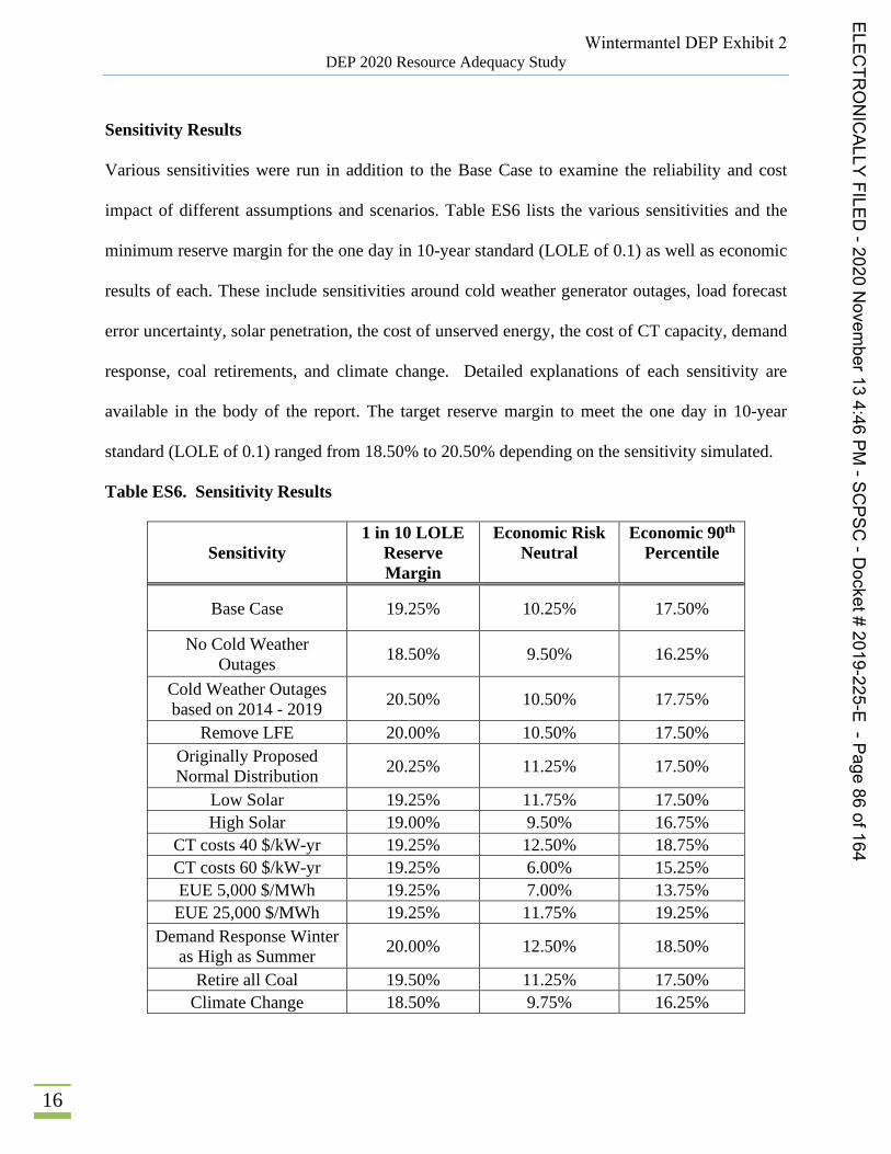
DEP 2020 Resource Adequacy Study
16
Sensitivity Results
Various sensitivities were run in addition to the Base Case to examine the reliability and cost
impact of different assumptions and scenarios. Table ES6 lists the various sensitivities and the
minimum reserve margin for the one day in 10-year standard (LOLE of 0.1) as well as economic
results of each. These include sensitivities around cold weather generator outages, load forecast
error uncertainty, solar penetration, the cost of unserved energy, the cost of CT capacity, demand
response, coal retirements, and climate change. Detailed explanations of each sensitivity are
available in the body of the report. The target reserve margin to meet the one day in 10-year
standard (LOLE of 0.1) ranged from 18.50% to 20.50% depending on the sensitivity simulated.
Table ES6. Sensitivity Results
Sensitivity 1 in 10 LOLE
Reserve Margin
Economic Risk Neutral
Economic 90th Percentile
Base Case 19.25% 10.25% 17.50%
No Cold Weather Outages 18.50% 9.50% 16.25%
Cold Weather Outages based on 2014 - 2019 20.50% 10.50% 17.75%
Remove LFE 20.00% 10.50% 17.50% Originally Proposed Normal Distribution 20.25% 11.25% 17.50%
Low Solar 19.25% 11.75% 17.50% High Solar 19.00% 9.50% 16.75%
CT costs 40 $/kW-yr 19.25% 12.50% 18.75% CT costs 60 $/kW-yr 19.25% 6.00% 15.25% EUE 5,000 $/MWh 19.25% 7.00% 13.75% EUE 25,000 $/MWh 19.25% 11.75% 19.25%
Demand Response Winter as High as Summer 20.00% 12.50% 18.50%
Retire all Coal 19.50% 11.25% 17.50% Climate Change 18.50% 9.75% 16.25%
Wintermantel DEP Exhibit 2ELEC
TRONICALLY
FILED-2020
Novem
ber134:46
PM-SC
PSC-D
ocket#2019-225-E
-Page86
of164

DEP 2020 Resource Adequacy Study
17
Recommendation
Based on the physical reliability results of the Island, Base Case, Combined Case, additional
sensitivities, as well as the results of the separate DEC Study, Astrapé recommends that DEP
continue to maintain a minimum 17% reserve margin for IRP purposes. This reserve margin
ensures reasonable reliability for customers. Astrapé recognizes that a standalone DEP utility
would require a 25.5% reserve margin to meet the one day in 10-year standard (LOLE of 0.1) and
even with market assistance, DEP would need to maintain a 19.25% reserve margin. Customers
expect electricity during extreme hot and cold weather conditions and maintaining a 17% reserve
margin is estimated to provide an LOLE of 0.12 events per year which is slightly less reliable than
the one day in 10-year standard (LOLE of 0.1). However, given the combined DEC and DEP
sensitivity resulting in a 16.75% reserve margin, and the 16% reserve margin required by DEC to
meet the one day in 10-year standard (LOLE of 0.1), Astrapé believes the 17% reserve margin as
a minimum target is still reasonable for planning purposes. Since the sensitivity results removing
all economic load forecast uncertainty increase the reserve margin to meet the 1 day in 10-year
standard, Astrapé believes this 17% minimum reserve margin should be used in the short- and
long-term planning process.
To be clear, even with 17% reserves, this does not mean that DEP will never be forced to shed
firm load during extreme conditions as DEP and its neighbors shift to reliance on intermittent and
energy limited resources such as storage and demand response. DEP has had several events in the
past few years where actual operating reserves were close to being exhausted even with higher
than 17% planning reserve margins. If not for non-firm external assistance, which this study
considers, firm load would have been shed. In addition, incorporation of tail end reliability risk in
Wintermantel DEP Exhibit 2ELEC
TRONICALLY
FILED-2020
Novem
ber134:46
PM-SC
PSC-D
ocket#2019-225-E
-Page87
of164

DEP 2020 Resource Adequacy Study
18
modeling should be from statistically and historically defendable methods; not from including
subjective risks that cannot be assigned probability. Astrapé’s approach has been to model the
system’s risks around weather, load, generator performance, and market assistance as accurately
as possible without overly conservative assumptions. Based on all results, Astrapé believes
planning to a 17% reserve margin is prudent from a physical reliability perspective and for small
increases in costs above the risk-neutral 10.25% reserve margin level, customers will experience
enhanced reliability and less rate volatility.
As the DEP resource portfolio changes with the addition of more intermittent resources and energy
limited resources, the 17% minimum reserve margin is sufficient as long as the Company has
accounted for the capacity value of solar and battery resources which changes as a function of
penetration. DEP should also monitor changes in the IRPs of neighboring utilities and the potential
impact on market assistance. Unless DEP observes seasonal risk shifting back to summer, the
17% reserve margin should be reasonable but should be re-evaluated as appropriate in future IRPs
and in future reliability studies. To ensure summer reliability is maintained, Astrapé recommends
not allowing the summer reserve margin to drop below 15%.16
16 Currently, if a winter target is maintained at 17%, summer reserves will be above 15%.
Wintermantel DEP Exhibit 2ELEC
TRONICALLY
FILED-2020
Novem
ber134:46
PM-SC
PSC-D
ocket#2019-225-E
-Page88
of164

DEP 2020 Resource Adequacy Study
19
I. List of Figures
Figure 1. Study Topology .......................................................................................................................... 22 Figure 2. DEP Summer Peak Weather Variability..................................................................................... 24 Figure 3. DEP Winter Peak Weather Variability ....................................................................................... 25 Figure 4. DEP Winter Calibration.............................................................................................................. 26 Figure 5. DEP Annual Energy Variability ................................................................................................. 27 Figure 6. Solar Map ................................................................................................................................... 34 Figure 7. Average August Output for Different Inverter Loading Ratios .................................................. 35 Figure 8. Scheduled Capacity .................................................................................................................... 36 Figure 9. Hydro Energy by Weather Year ................................................................................................. 37 Figure 10. Operating Reserve Demand Curve (ORDC) ............................................................................ 40 Figure 11. Base Case Risk Neutral Economic Results .............................................................................. 49 Figure 12. Cumulative Probability Curves ................................................................................................ 51 Figure 13. Total System Costs by Reserve Margin.................................................................................... 53
Wintermantel DEP Exhibit 2ELEC
TRONICALLY
FILED-2020
Novem
ber134:46
PM-SC
PSC-D
ocket#2019-225-E
-Page89
of164

DEP 2020 Resource Adequacy Study
20
II. List of Tables
Table 1. 2024 Forecast: DEP Seasonal Peak (MW) .................................................................................. 23 Table 2. External Region Summer Load Diversity .................................................................................... 28 Table 3. External Region Winter Load Diversity ...................................................................................... 28 Table 4. Load Forecast Error ..................................................................................................................... 29 Table 5. DEP Baseload and Intermediate Resources ................................................................................. 30 Table 6. DEP Peaking Resources ............................................................................................................... 30 Table 7. DEP Renewable Resources Excluding Existing Hydro ............................................................... 33 Table 8. DEP Demand Response Modeling ............................................................................................... 38 Table 9. Unserved Energy Costs / Value of Lost Load .............................................................................. 41 Table 10. Case Probability Example .......................................................................................................... 42 Table 11. Relationship Between Winter and Summer Reserve Margin Levels ......................................... 44 Table 12. Island Physical Reliability Results ............................................................................................. 45 Table 13. Base Case Physical Reliability Results ...................................................................................... 46 Table 14. Reliability Metrics: Base Case ................................................................................................... 48 Table 15. Annual Customer Costs vs LOLE .............................................................................................. 52 Table 16. No Cold Weather Outage Results .............................................................................................. 55 Table 17. Cold Weather Outages Based on 2014-2019 Results ................................................................ 55 Table 18. Remove LFE Results ................................................................................................................. 56 Table 19. Originally Proposed LFE Distribution Results .......................................................................... 56 Table 20. Low Solar Results ...................................................................................................................... 57 Table 21. High Solar Results ..................................................................................................................... 57 Table 22. Demand Response Results ......................................................................................................... 58 Table 23. No Coal Results ......................................................................................................................... 58 Table 24. Climate Change Results ............................................................................................................. 59 Table 25. Economic Sensitivities ............................................................................................................... 60 Table 26. Combined Case Results ............................................................................................................. 61
Wintermantel DEP Exhibit 2ELEC
TRONICALLY
FILED-2020
Novem
ber134:46
PM-SC
PSC-D
ocket#2019-225-E
-Page90
of164

DEP 2020 Resource Adequacy Study
21
III. Input Assumptions
A. Study Year
The selected study year is 202417. The SERVM simulation results are broadly applicable to future
years assuming that resource mixes and market structures do not change in a manner that shifts the
reliability risk to a different season or different time of day.
B. Study Topology
Figure 1 shows the study topology that was used for the Resource Adequacy Study. DEP was
modeled in two interconnect zones: (1) DEP – E and (2) DEP – W. While market assistance is not
as dependable as resources that are utility owned or have firm contracts, Astrapé believes it is
appropriate to capture the load diversity and generator outage diversity that DEP has with its
neighbors. For this study, the DEP system was modeled with eight surrounding regions. The
surrounding regions captured in the modeling included Duke Energy Carolinas (DEC), Tennessee
Valley Authority (TVA), Southern Company (SOCO), PJM West & PJM South, Yadkin (YAD),
Dominion Energy South Carolina (formally known as South Carolina Electric & Gas (SCEG)),
and Santee Cooper (SC). SERVM uses a pipe and bubble representation in which energy can be
shared based on economics but subject to transmission constraints.
17 The year 2024 was chosen because it is four years into the future which is indicative of the amount of time needed to permit and construct a new generating facility.
Wintermantel DEP Exhibit 2ELEC
TRONICALLY
FILED-2020
Novem
ber134:46
PM-SC
PSC-D
ocket#2019-225-E
-Page91
of164

DEP 2020 Resource Adequacy Study
22
Figure 1. Study Topology
Confidential Appendix Table CA1 displays the DEP import capability from surrounding regions
including the amount set aside for Transmission Reliability Margin (TRM).
C. Load Modeling
Table 1 displays SERVM’s modeled seasonal peak forecast net of energy efficiency programs for
2024.
Wintermantel DEP Exhibit 2ELEC
TRONICALLY
FILED-2020
Novem
ber134:46
PM-SC
PSC-D
ocket#2019-225-E
-Page92
of164
PJM
'est
PJM
South
~ ~
DEC
YAD
DEP-E,
i soco i
SCEG 'C

DEP 2020 Resource Adequacy Study
23
Table 1. 2024 Forecast: DEP Seasonal Peak (MW)
DEP-E Non- Coincident
DEP-W Non- Coincident Combined Coincident
2024 Summer 12,227 879 13,042
2024 Winter 13,390 1,175 14,431
To model the effects of weather uncertainty, thirty-nine historical weather years (1980 - 2018)
were developed to reflect the impact of weather on load. Based on the last five years of historical
weather and load18, a neural network program was used to develop relationships between weather
observations and load. The historical weather consisted of hourly temperatures from five weather
stations across the DEP service territory. The weather stations included Raleigh, NC, Wilmington,
NC, Fayetteville, NC, Asheville, NC, and Columbia, SC. Other inputs into the neural net model
consisted of hour of week, eight hour rolling average temperatures, twenty-four hour rolling
average temperatures, and forty-eight hour rolling average temperatures. Different weather to load
relationships were built for the summer, winter, and shoulder seasons. These relationships were
then applied to the last thirty-nine years of weather to develop thirty-nine synthetic load shapes for
2024. Equal probabilities were given to each of the thirty-nine load shapes in the simulation. The
synthetic load shapes were scaled to align the normal summer and winter peaks to the Company’s
projected thirty-year weather normal load forecast for 2024.
Figures 2 and 3 show the results of the 2014-2019 weather load modeling by displaying the peak
load variance for both the summer and winter seasons. The y-axis represents the percentage
18 The historical load included years 2014 through September of 2019.
Wintermantel DEP Exhibit 2ELEC
TRONICALLY
FILED-2020
Novem
ber134:46
PM-SC
PSC-D
ocket#2019-225-E
-Page93
of164

DEP 2020 Resource Adequacy Study
24
deviation from the average peak. For example, the 1985 synthetic load shape would result in a
summer peak load approximately 4.7% below normal and a winter peak load approximately 21.1%
above normal. Thus, the bars represent the variance in projected peak loads based on weather
experienced during the historic weather years. It should be noted that the variance for winter is
much greater than summer. As an example, extreme cold temperatures can cause load to spike
from additional electric strip heating. The highest summer temperatures typically are only a few
degrees above the expected highest temperature and therefore do not produce as much peak load
variation.
Figure 2. DEP Summer Peak Weather Variability
Wintermantel DEP Exhibit 2ELEC
TRONICALLY
FILED-2020
Novem
ber134:46
PM-SC
PSC-D
ocket#2019-225-E
-Page94
of164
2.096
E0+ o.oxE0
@ -2.0%
-4.0%
-6.0%
-8.0%ClCO CO CO CO CO CO CO CO CO CO Ol (O Ol Ol O Ol CO Ol Ol 0 0 O 0 O O O O 0 O 00 Ol 0 O 0 0 0 (h Ol 0 0 0 0 Ol 0 Ol 0 0 Ol 0 0 0 0 0 0 0 0 0 0 0 0 0 0 0 0 0 0 0 0
CC C( OI I I CC C( I C( I CC I CC I OI C( OI CC
Weather Year

DEP 2020 Resource Adequacy Study
25
Figure 3. DEP Winter Peak Weather Variability
Figure 4 shows a daily peak load comparison of the synthetic load shapes and DEP history as a
function of temperature. The predicted values align well with the history. Because recent
historical observations only recorded a single minimum temperature of seven degrees Fahrenheit,
Astrapé estimated the extrapolation for extreme cold weather days using regression analysis on the
historical data. This figure highlights that the frequency of cold weather events is captured as it
has been seen in history. The worst day seen in the thirty-nine year history was negative three
degrees Fahrenheit. As shown in the following figure, the load associated with this day was capped
very close to the six degree Fahrenheit day to assume saturation, however, the Company is
skeptical that there would be much saturation on cold winter days because customers have
continued to turn on additional heating options such as space heaters, ovens, etc.
Wintermantel DEP Exhibit 2ELEC
TRONICALLY
FILED-2020
Novem
ber134:46
PM-SC
PSC-D
ocket#2019-225-E
-Page95
of164
25.0%
20.0%
15.0%
10.0%
5.0%
ZE
0.0%
g-5.0%
-10.0%
-15.0%
-20.0%0 m m m m 0 I m 0 0 m m m 0 I 0 a 0 m m m 0 I «I 0 0 m m m m 0 I «Ico co co co co co co co a\ co al co 0 al m al al m co al 0 0 0 0 0 0 0 0 0 0a Ol 0 0 O al 0 O 0 a O 0 a 0 0 a 0 0 a 0 0 0 0 0 0 0 0 0 0 0 0 0 0 0 0 0 0 0 0cl OI ca ca OI ca ca OI al ca cl al ca cl al ca cl al ca
Weather Year

DEP 2020 Resource Adequacy Study
26
Figure 4. DEP Winter Calibration
The energy variation is lower than peak variation across the weather years as expected. As shown
in Figure 5, 2010 was an extreme year in total energy due to persistent severe temperatures across
the summer and yet the deviation from average was only 6%.
Wintermantel DEP Exhibit 2ELEC
TRONICALLY
FILED-2020
Novem
ber134:46
PM-SC
PSC-D
ocket#2019-225-E
-Page96
of164
19,5DD
17,500
15,500
13,500
O11,500
te
2'I 9,500tn
7,500
5,500
3,500-5 1D
Dally Min Temperature(ep)
Synthetic ~ DEP Htstottcet
15 20 25

DEP 2020 Resource Adequacy Study
27
Figure 5. DEP Annual Energy Variability
The synthetic shapes described above were then scaled to the forecasted seasonal energy and peaks
within SERVM. Because DEP’s load forecast is based on thirty years of weather, the shapes were
scaled so that the average of the last thirty years equaled the forecast.
Synthetic loads for each external region were developed in a similar manner as the DEP loads. A
relationship between hourly weather and publicly available hourly load19 was developed based on
recent history, and then this relationship was applied to thirty-nine years of weather data to develop
thirty-nine synthetic load shapes. Tables 2 and 3 show the resulting weather diversity between
DEP and external regions for both summer and winter loads. When the system, which includes all
19 Federal Energy Regulatory Commission (FERC) 714 Forms were accessed during January of 2020 to pull hourly historical load for all neighboring regions.
Wintermantel DEP Exhibit 2ELEC
TRONICALLY
FILED-2020
Novem
ber134:46
PM-SC
PSC-D
ocket#2019-225-E
-Page97
of164
8.00%
6.00%
4.00%
E0Z 2.00%E0
g0.00%
-2.00%
-4.00%0 m m m 0 I m 0 0 m m m m 0 I 0 a 0 m m m 0 I «I 0 0 m m m m 0 I «Ico co co co co co co co co co al co a al 0 al al 0 co al 0 0 0 0 0 0 0 0 0 00 0 a 0 0 0 O Ol 0 0 O al a O 0 a 0 0 a 0 0 0 0 0 0 0 0 0 0 0 0 0 0 0 0 0 0 0 0cl OI ca cl OI ca cl ol ol cl cl ol ca cl OI ca cl OI ca
Weather Year

DEP 2020 Resource Adequacy Study
28
regions in the study, is at its winter peak, the individual regions are approximately 2% - 9% below
their non-coincidental peak load on average over the thirty-nine year period, resulting in an average
system diversity of 4.7%. When DEP is at its winter peak load, DEC is 2.7% below its peak load
on average while other regions are approximately 3 - 9% below their winter peak loads on average.
Similar values are seen during the summer.
Table 2. External Region Summer Load Diversity
Load Diversity (% below non coincident average
peak) DEC DEP SOCO TVA SC SCEG PJM
S PJM
W System
At System Coincident Peak 3.4% 3.8% 5.2% 4.2% 6.8% 7.0% 3.7% 1.4% N/A
At DEP Peak 2.0% N/A 8.0% 6.8% 7.3% 7.1% 5.7% 9.6% 3.6% Table 3. External Region Winter Load Diversity
Load Diversity (% below non coincident average
peak) DEC DEP SOCO TVA SC SCEG PJM
S PJM
W System
At System Coincident Peak 2.5% 2.8% 2.8% 5.8% 8.9% 4.8% 6.9% 3.2% N/A
At DEP Peak 2.7% N/A 4.7% 8.4% 6.7% 3.0% 5.2% 8.9% 2.4%
D. Economic Load Forecast Error
Economic load forecast error multipliers were developed to isolate the economic uncertainty that
Duke has in its four year ahead load forecasts. Four years is an approximation for the amount of
time it takes to build a new resource or otherwise significantly change resource plans. To estimate
the economic load forecast error, the difference between Congressional Budget Office (CBO)
Gross Domestic Product (GDP) forecasts four years ahead and actual data was fit to a distribution
which weighted over-forecasting more heavily than under-forecasting load20. This was a direct
20 CBO's Economic Forecasting Record: 2017 Update. www.cbo.gov/publication/53090 www.cbo.gov/publication/53090
Wintermantel DEP Exhibit 2ELEC
TRONICALLY
FILED-2020
Novem
ber134:46
PM-SC
PSC-D
ocket#2019-225-E
-Page98
of164

DEP 2020 Resource Adequacy Study
29
change accepted as part of the feedback in stakeholder meetings.21 Because electric load grows at
a slower rate than GDP, a 40% multiplier was applied to the raw CBO forecast error distribution.
Table 4 shows the economic load forecast multipliers and associated probabilities. As an
illustration, 25% of the time, it is expected that load will be over-forecasted by 2.7% four years
out. Within the simulations, when DEP over-forecasts load, the external regions also over-forecast
load. The SERVM model utilized each of the thirty-nine weather years and applied each of these
five load forecast error points to create 195 different load scenarios. Each weather year was given
an equal probability of occurrence.
Table 4. Load Forecast Error
Load Forecast Error Multipliers Probability %
0.958 10.0% 0.973 25.0% 1.00 40.0% 1.02 15.0% 1.031 10.0%
E. Conventional Thermal Resources
DEP resources are outlined in Tables 5 and 6 and represent summer ratings and winter ratings. All
thermal resources are committed and dispatched to load economically. The capacities of the units
are defined as a function of temperature in the simulations. Full winter rating is achieved at 35°F
and below and summer rating is assumed for 95° and above. For temperatures in between 35°F
and 95°F, a simple linear regression between the summer and winter rating was utilized for each
unit.
21 Including the economic load forecast uncertainty actually results in a lower reserve margin compared to a scenario that excludes the load forecast uncertainty since over-forecasting load is weighted more heavily than under-forecasting load.
Wintermantel DEP Exhibit 2ELEC
TRONICALLY
FILED-2020
Novem
ber134:46
PM-SC
PSC-D
ocket#2019-225-E
-Page99
of164

DEP 2020 Resource Adequacy Study
30
Table 5. DEP Baseload and Intermediate Resources
Unit Name Resource
Type
Summer Capacity
(MW)
Winter Capacity
(MW) Unit Name Resource Type
Summer Capacity
(MW)
Winter Capacity
(MW)
Mayo 1 Coal 727 746 Smith CC 4 NG - Combined
Cycle 476 570
Roxboro 1 Coal 379 380 Smith CC 5 NG - Combined
Cycle 489 589
Roxboro 2 Coal 671 673 Smith CC
5_DF/PAG NG – Duct
Firing/Power Aug 65/43 61/30
Roxboro 3 Coal 694 698 Lee/Wayne CC 1 NG - Combined
Cycle 794 990
Roxboro 4 Coal 698 711 Lee/Wayne CC
1_DF NG – Duct Firing 94 69
Brunswick 1 Nuclear 938 975 Sutton CC 1 NG - Combined
Cycle 536 658
Brunswick 2 Nuclear 932 953 Sutton CC 1_DF NG - Duct Firing 71 61
Harris 1 Nuclear 964 1009 Asheville CC NG - Combined
Cycle 496 560
Robinson 2 Nuclear 741 797 Table 6. DEP Peaking Resources
Unit Name Resource
Type
Summer Capacity
(MW)
Winter Capacity
(MW) Unit Name Resource
Type
Summer Capacity
(MW) Winter Capacity
(MW)
Blewett CT 1 Oil
Peaker 13 17 Smith CT 3 NG Peaker 155 185
Blewett CT 2 Oil
Peaker 13 17 Smith CT 4 NG Peaker 159 186
Blewett CT 3 Oil
Peaker 13 17 Smith CT 6 NG Peaker 155 187
Blewett CT 4 Oil
Peaker 13 17 Wayne CT 1 Oil Peaker 177 192
Asheville CT 3 NG
Peaker 160 185 Wayne CT 2 Oil Peaker 174 192
Asheville CT 4
Natural Gas
Peaker 160 185 Wayne CT 3 Oil/NG Peaker 173 193
Darl CT 12 NG
Peaker 118 133 Wayne CT 4 Oil/NG Peaker 170 191
Darl CT 13 NG
Peaker 116 133 Wayne CT 5 Oil/NG Peaker 163 195
LM6000 (Sutton)
NG Peaker 39 49
Weatherspoon CT 1 Oil Peaker 31 41
LM6000 (Sutton)
NG Peaker 39 49
Weatherspoon CT 2 Oil Peaker 31 41
Smith CT 1 NG
Peaker 157 189 Weatherspoon
CT 3 Oil Peaker 32 41
Smith CT 2 NG
Peaker 156 187 Weatherspoon
CT 4 Oil Peaker 30 41
Wintermantel DEP Exhibit 2ELEC
TRONICALLY
FILED-2020
Novem
ber134:46
PM-SC
PSC-D
ocket#2019-225-E
-Page100
of164

DEP 2020 Resource Adequacy Study
31
DEP purchase contracts were modeled as shown in Confidential Appendix Table CA2. These
resources were treated as traditional thermal resources and counted towards reserve margin.
Confidential Appendix Table CA3 shows the fuel prices used in the study for DEP and its
neighboring power systems.
F. Unit Outage Data
Unlike typical production cost models, SERVM does not use an Equivalent Forced Outage Rate
(EFOR) for each unit as an input. Instead, historical Generating Availability Data System (GADS)
data events for the period 2014-2019 are entered in for each unit and SERVM randomly draws
from these events to simulate the unit outages. Units without historical data use history from
similar technologies. The events are entered using the following variables:
Full Outage Modeling Time-to-Repair Hours Time-to-Fail Hours Partial Outage Modeling Partial Outage Time-to-Repair Hours Partial Outage Derate Percentage Partial Outage Time-to-Fail Hours Maintenance Outages Maintenance Outage Rate - % of time in a month that the unit will be on maintenance outage. SERVM uses this percentage and schedules the maintenance outages during off peak periods. Planned Outages The actual schedule for 2024 was used.
To illustrate the outage logic, assume that from 2014 – 2019, a generator had 15 full outage events
and 30 partial outage events reported in the GADS data. The Time-to-Repair and Time-to-Fail
between each event is calculated from the GADS data. These multiple Time-to-Repair and Time-
Wintermantel DEP Exhibit 2ELEC
TRONICALLY
FILED-2020
Novem
ber134:46
PM-SC
PSC-D
ocket#2019-225-E
-Page101
of164

DEP 2020 Resource Adequacy Study
32
to-Fail inputs are the distributions used by SERVM. Because there may be seasonal variances in
EFOR, the data is broken up into seasons such that there is a set of Time-to-Repair and Time-to-
Fail inputs for summer, shoulder, and winter, based on history. Further, assume the generator is
online in hour 1 of the simulation. SERVM will randomly draw both a full outage and partial
outage Time-to-Fail value from the distributions provided. Once the unit has been economically
dispatched for that amount of time, it will fail. A partial outage will be triggered first if the
selected Time-to-Fail value is lower than the selected full outage Time-to-Fail value. Next, the
model will draw a Time-to-Repair value from the distribution and be on outage for that number of
hours. When the repair is complete it will draw a new Time-to-Fail value. The process repeats until
the end of the iteration when it will begin again for the subsequent iteration. The full outage
counters and partial outage counters run in parallel. This more detailed modeling is important to
capture the tails of the distribution that a simple convolution method would not capture.
Confidential Appendix Table CA4 shows system peak season Equivalent Forced Outage Rate
(EFOR) for the system and by unit.
The most important aspect of unit performance modeling in resource adequacy studies is the
cumulative MW offline distribution. Most service reliability problems are due to significant
coincident outages. Confidential Appendix Figure CA1 shows the distribution of modeled system
outages as a percentage of time modeled and compared well with actual historical data.
Additional analysis was performed to understand the impact cold temperatures have on system
outages. Confidential Appendix Figures CA2 and CA3 show the difference in cold weather
outages during the 2014-2019 period and the 2016-2019 period. The 2014-2019 period showed
Wintermantel DEP Exhibit 2ELEC
TRONICALLY
FILED-2020
Novem
ber134:46
PM-SC
PSC-D
ocket#2019-225-E
-Page102
of164

DEP 2020 Resource Adequacy Study
33
more events than the 2016-2019 period which is logical because Duke Energy has put practices in
place to enhance reliability during these periods, however the 2016 – 2019 data shows some events
still occur. The average capacity offline below 10 degrees for DEC and DEP combined was 400
MW. Astrapé split this value by peak load ratio and included 140 MW in the DEP Study and 260
MW in the DEC Study at temperatures below 10 degrees. Sensitivities were performed with the
cold weather outages removed and increased to match the 2014 – 2019 dataset which showed an
average of 800 MW offline on days below 10 degrees. The MWs offline during the 10 coldest days
can be seen in Confidential Appendix Table CA5. The outages shown are only events that included
some type of freezing or cold weather problem as part of the description in the outage event.
G. Solar and Battery Modeling
Table 7 shows the solar and battery resources captured in the study.
Table 7. DEP Renewable Resources Excluding Existing Hydro
Unit Type
Summer Capacity
(MW)
Winter Capacity (MW)
Modeling
Utility Owned-Fixed 141 141 Hourly Profiles
Transition-Fixed 2,432 2,432 Hourly Profiles
Competitive Procurement of Renewable Energy
(CPRE) Tranche 1
Fixed 40%/Tracking 60% 86 86 Hourly Profiles
Future Solar
Fixed 40%/Tracking 60% 1,448 1,448 Hourly Profiles
Total Solar 4,107 4,107
Total Battery 83 83 Modeled as energy arbitrage
Wintermantel DEP Exhibit 2ELEC
TRONICALLY
FILED-2020
Novem
ber134:46
PM-SC
PSC-D
ocket#2019-225-E
-Page103
of164

DEP 2020 Resource Adequacy Study
34
The solar units were simulated with thirty-nine solar shapes representing thirty-nine years of
weather. The solar shapes were developed by Astrapé from data downloaded from the National
Renewable Energy Laboratory (NREL) National Solar Radiation Database (NSRDB) Data
Viewer. The data was then input into NREL’s System Advisor Model (SAM) for each year and
county to generate hourly profiles for both fixed and tracking solar profiles. The solar capacity
was given 20% credit in the summer and 1% in the winter for reserve margin calculations based
on the 2018 Solar Capacity Value Study. Figure 6 shows the county locations that were used and
Figure 7 shows the average August output for different fixed-tilt and single-axis-tracking inverter
loading ratios.
Figure 6. Solar Map
Wintermantel DEP Exhibit 2ELEC
TRONICALLY
FILED-2020
Novem
ber134:46
PM-SC
PSC-D
ocket#2019-225-E
-Page104
of164

DEP 2020 Resource Adequacy Study
35
Figure 7. Average August Output for Different Inverter Loading Ratios
H. Hydro Modeling
The scheduled hydro is used for shaving the daily peak load but also includes minimum flow
requirements. Figure 8 shows the total breakdown of scheduled hydro based on the last thirty-nine
years of weather.
Wintermantel DEP Exhibit 2ELEC
TRONICALLY
FILED-2020
Novem
ber134:46
PM-SC
PSC-D
ocket#2019-225-E
-Page105
of164
80
70
— 60
5 500
o 40Ill
.~ 30
Eo 20Z
10
10 15 20 25
Hour of Day

DEP 2020 Resource Adequacy Study
36
Figure 8. Scheduled Capacity
Figure 9 demonstrates the variation of hydro energy by weather year which is input into the model.
The lower rainfall years such as 2001, 2007, and 2008 are captured in the reliability model with
lower peak shaving as shown in Figure 9.
Wintermantel DEP Exhibit 2ELEC
TRONICALLY
FILED-2020
Novem
ber134:46
PM-SC
PSC-D
ocket#2019-225-E
-Page106
of164
230
220
5 210
U
ca 200
0~ 190c0
180E
'x 170
160
150a &De c ZS e~00&c EE a Z Dec c & i~ 0 0 sec ZZ cu 00&c & a~a Z gc 2& a~00&c EZ cu Z
D — oc fDhcDUDDD —D'0 oh — UocfDhcceco — Dao hhcco(DQcococoN 'ocococococo 'ee eluee eooloee 'o00000000 00 ~l'' o I0V eeaaCOCOCOVCOCO0 ~CO DeSCOVCO 0 h OUCUOONCOVCOCoe VNCUul4 IPCO~+gee
Date

DEP 2020 Resource Adequacy Study
37
Figure 9. Hydro Energy by Weather Year
I. Demand Response Modeling
Demand response programs are modeled as resources in the simulations. They are modeled with
specific contract limits including hours per year, days per week, and hours per day constraints. For
this study, 1,001 MW of summer capacity and 461 MW of winter capacity were included as shown
in Table 8. To ensure these resources were called after conventional generation, a $2,000/MWh
strike price was included.
Wintermantel DEP Exhibit 2ELEC
TRONICALLY
FILED-2020
Novem
ber134:46
PM-SC
PSC-D
ocket#2019-225-E
-Page107
of164
1,200
1,000
800
IO600
0IO0
z Coo
0 0 I I R R R t I t 0 0 0 tt II 4 tt 4 4 IO I 0 0 tt tt tt 4 I 4 IJ IOl D ID IO IO D Ul Ol O\ Ol IO ID Ol Ol Cl IO ID IO Ol II Q lj 8 8 Cj I3 8 I3 P 8 CI CI CI CI CI It 0 Cl 00 X 0 4 ID 4 0 N I 6 0 4 I Ot le 6 0 I 4 0 6 0 V I
Weather Year

DEP 2020 Resource Adequacy Study
38
Table 8. DEP Demand Response Modeling
Region Program Summer Capacity
(MW) Winter Capacity
(MW) Hours Per
Year Days Per
Week Hours Per
Day
DEP EnergyWise Home 430 22 60 7 4
DEP EnergyWise
Business 22 2 60 7 4
DEP Demand Response
Automation 44 24 80 7 8
DEP Large Load Curtailable 265 245 100 7 8
DEP Distribution System Demand Response 240 168 100 7 8
Total DEP 1,001 461
J. Operating Reserve Requirements
The operating reserves assumed for DEP are shown below. SERVM commits to this level of
operating reserves in all hours. However, all operating reserves except for the 150 MW of
regulation are allowed to be depleted during a firm load shed event.
Regulation Up/Down: 150 MW Spinning Requirement: 200 MW Non-Spin Requirement: 200 MW Additional Load Following Due to Intermittent Resources in 2024: Hourly values were
used based on a 12x24 profile provided by Duke Energy from its internal modeling.
K. External Assistance Modeling
The external market plays a significant role in planning for resource adequacy. If several of the
DEP resources were experiencing an outage at the same time, and DEP did not have access to
surrounding markets, there is a high likelihood of unserved load. To capture a reasonable amount
Wintermantel DEP Exhibit 2ELEC
TRONICALLY
FILED-2020
Novem
ber134:46
PM-SC
PSC-D
ocket#2019-225-E
-Page108
of164

DEP 2020 Resource Adequacy Study
39
of assistance from surrounding neighbors, each neighbor was modeled at the one day in 10-year
standard (LOLE of 0.1) level representing the target for many entities. By modeling in this manner,
only weather diversity and generator outage diversity benefits are captured. The market
representation used in SERVM is based on Astrapé’s proprietary dataset which is developed based
on FERC Forms, Energy Information Administration (EIA) Forms, and reviews of IRP
information from neighboring regions. To ensure purchases in the model compared well in
magnitude to historical data, the years 2015 and 2018 were simulated since they reflected cold
weather years with high winter peaks. Figure CA4 in the confidential appendix shows that
calibration with purchases on the y-axis and load on the x-axis for the 2015 and 2018 weather
years. The actual purchases and modeled results show DEP purchases significant capacity during
high load hours during these years.
The cost of transfers between regions is based on marginal costs. In cases where a region is short
of resources, scarcity pricing is added to the marginal costs. As a region’s hourly reserves approach
zero, the scarcity pricing for that region increases. Figure 10 shows the scarcity pricing curve that
was used in the simulations. It should be noted that the frequency of these scarcity prices is very
low because in the majority of hours, there is plenty of capacity to meet load after the market has
cleared22.
22The market clearing algorithm within SERVM attempts to get all regions to the same price subject to transmission constraints. So, if a region’s original price is $3,000/MWh based on the conditions and scarcity pricing in that region alone, it is highly probable that a surrounding region will provide enough capacity to that region to bring prices down to reasonable levels.
Wintermantel DEP Exhibit 2ELEC
TRONICALLY
FILED-2020
Novem
ber134:46
PM-SC
PSC-D
ocket#2019-225-E
-Page109
of164

DEP 2020 Resource Adequacy Study
40
Figure 10. Operating Reserve Demand Curve (ORDC)
L. Cost of Unserved Energy
Unserved energy costs were derived from national studies completed for the Department of Energy
(DOE) in 200323 and 200924, along with three other studies performed25 previously by other
consultants. The DOE studies were compilations of other surveys performed by utilities over the
last two decades. All studies split the customer class categories into residential, commercial, and
industrial. The values were then applied to the actual DEP customer class mix to develop a wide
23 https://eta-publications.lbl.gov/sites/default/files/lbnl-54365.pdf https://eta-publications.lbl.gov/sites/default/files/lbnl-54365.pdf 24 https://eta-publications.lbl.gov/sites/default/files/lbnl-2132e.pdf https://eta-publications.lbl.gov/sites/default/files/lbnl-2132e.pdf 25 https://pdfs.semanticscholar.org/544b/d740304b64752b451d749221a00eede4c700.pdf Peter Cramton, Jeffrey Lien. Value of Lost Load. February 14, 2000.
Wintermantel DEP Exhibit 2ELEC
TRONICALLY
FILED-2020
Novem
ber134:46
PM-SC
PSC-D
ocket#2019-225-E
-Page110
of164
3500
3000
2500
& 2000
IJ 1500
1000
500
0
0 10 15
Operating Reserve%20 25 30

DEP 2020 Resource Adequacy Study
41
range of costs for unserved energy. Table 9 shows those results. Because expected unserved
energy costs are so low near the economic optimum reserve margin, this value, while high in
magnitude, is not a significant driver in the economic analysis. Since the public estimates ranged
significantly, DEP used $16,450/MWh for the Base Case in 2024, and sensitivities were performed
around this value from $5,000 MWh to $25,000 MWh to understand the impact.
Table 9. Unserved Energy Costs / Value of Lost Load
M. System Capacity Carrying Costs
The study assumes that the cheapest marginal resource is utilized to calculate the carrying cost of
additional capacity. The cost of carrying incremental reserves was based on the capital and FOM
of a new simple cycle natural gas Combustion Turbine (CT) consistent with the Company’s IRP
assumptions. For the study, the cost of each additional kW of reserves can be found in Confidential
Appendix Table CA6. The additional CT units were forced to have a 5% EFOR in the simulations
and used to vary reserve margin in the study.
Wintermantel DEP Exhibit 2ELEC
TRONICALLY
FILED-2020
Novem
ber134:46
PM-SC
PSC-D
ocket#2019-225-E
-Page111
of164
W' s
2003 DOE Study
2024 5lcWh2009 DOE Study Chnstiansea Assomates Bilgnton and Wacker Karugu aad Agaa
2024 S'kWh 2024 SdcWh 2024 SlcWh 2024 SlcWh
Residenual
Commercial
ladustrial
43%33%24%
1 57
35 54
20 51
1.50
109.23
32.53
3.1222.3711.59
2.7323 2423.24
1 26
24 74
58 65
Weighted Average 5'kWh 17.31 44 55 11 50 14 38 22 60
Average S'kWhAverage S kV 'h exduding
the 2009 DOE Study
22 07
16 45

DEP 2020 Resource Adequacy Study
42
IV. Simulation Methodology Since most reliability events are high impact, low probability events, a large number of scenarios
must be considered. For DEP, SERVM utilized thirty-nine years of historical weather and load
shapes, five points of economic load growth forecast error, and fifteen iterations of unit outage
draws for each scenario to represent a distribution of realistic scenarios. The number of yearly
simulation cases equals 39 weather years * 5 load forecast errors * 15 unit outage iterations =
2,925 total iterations for the Base Case. This Base Case, comprised of 2,925 total iterations, was
re-run at different reserve margin levels by varying the amount of CT capacity.
A. Case Probabilities
An example of probabilities given for each case is shown in Table 10. Each weather year is given
equal probability and each weather year is multiplied by the probability of each load forecast error
point to calculate the case probability.
Table 10. Case Probability Example
Weather Year
Weather Year Probability
(%)
Load multipliers Due to Load Economic Forecast
Error (%)
Load Economic Forecast Error
Probability (%)
Case Probability
(%) 1980 2.56 95.8 10 0.256 1980 2.56 97.3 25 0.64 1980 2.56 100 40 1.024 1980 2.56 102 15 0.384 1980 2.56 103.1 10 0.256 1981 2.56 95.8 10 0.256 1981 2.56 97.3 25 0.64 1981 2.56 100 40 1.024 1981 2.56 102 15 0.384 1981 2.56 103.1 10 0.256 1982 2.56 95.8 10 0.256 1982 2.56 97.3 25 0.64 1982 2.56 100 40 1.024 1982 2.56 102 15 0.384
Wintermantel DEP Exhibit 2ELEC
TRONICALLY
FILED-2020
Novem
ber134:46
PM-SC
PSC-D
ocket#2019-225-E
-Page112
of164

DEP 2020 Resource Adequacy Study
43
1982 2.56 103.1 10 0.256 ... ... ... ... ... ... ... ... ... ...
2018 2.56 103.1 10 0.256
Total 100
For this study, LOLE is defined in number of days per year and is calculated for each of the 195
load cases and weighted based on probability. When counting LOLE events, only one event is
counted per day even if an event occurs early in the day and then again later in the day. Across
the industry, the traditional 1 day in 10 year LOLE standard is defined as 0.1 LOLE. Additional
reliability metrics calculated are Loss of Load Hours (LOLH) in hours per year and Expected
Unserved Energy (EUE) in MWh.
Total system energy costs are defined as the following for each region: 𝑃𝑃𝑃𝑃𝑃𝑃𝑃𝑃𝑃𝑃𝑃𝑃𝑃𝑃𝑃𝑃𝑃𝑃𝑃𝑃 𝐶𝐶𝑃𝑃𝐶𝐶𝑃𝑃𝐶𝐶 (𝐹𝐹𝑃𝑃𝐹𝐹𝐹𝐹 𝐵𝐵𝑃𝑃𝑃𝑃𝑃𝑃 + 𝑉𝑉𝑉𝑉𝑃𝑃𝑃𝑃𝑉𝑉𝑉𝑉𝐹𝐹𝐹𝐹 𝑂𝑂&𝑀𝑀) + 𝑃𝑃𝑃𝑃𝑃𝑃𝑃𝑃ℎ𝑉𝑉𝐶𝐶𝐹𝐹 𝐶𝐶𝑃𝑃𝐶𝐶𝑃𝑃𝐶𝐶 − 𝑆𝑆𝑉𝑉𝐹𝐹𝐹𝐹𝐶𝐶 𝑅𝑅𝐹𝐹𝑅𝑅𝐹𝐹𝑃𝑃𝑃𝑃𝐹𝐹
+ 𝐿𝐿𝑃𝑃𝐶𝐶𝐶𝐶 𝑃𝑃𝑜𝑜 𝑅𝑅𝐹𝐹𝐶𝐶𝐹𝐹𝑃𝑃𝑅𝑅𝐹𝐹𝐶𝐶 + 𝐶𝐶𝑃𝑃𝐶𝐶𝑃𝑃 𝑃𝑃𝑜𝑜 𝑈𝑈𝑃𝑃𝐶𝐶𝐹𝐹𝑃𝑃𝑅𝑅𝐹𝐹𝑃𝑃 𝐸𝐸𝑃𝑃𝐹𝐹𝑃𝑃𝐸𝐸𝐸𝐸
These components are calculated for each case and weighted based on probability to calculate total
system energy costs for each scenario simulated. Loss of Reserves costs recognize the additional
risk of depleting operating reserves and are costed out at the ORDC curve when they occur. As
shown in the results these costs are almost negligible. The cost of unserved energy is simply the
MWh of load shed multiplied by the value of lost load. System capacity costs are calculated
separately outside of the SERVM model using the economic carrying cost of a new CT.
Wintermantel DEP Exhibit 2ELEC
TRONICALLY
FILED-2020
Novem
ber134:46
PM-SC
PSC-D
ocket#2019-225-E
-Page113
of164

DEP 2020 Resource Adequacy Study
44
B. Reserve Margin Definition
For this study, winter and summer reserve margins are defined as the following:
o (Resources – Demand) / Demand
Demand is 50/50 peak forecast
Demand response programs are included as resources and not subtracted from demand
Solar capacity is counted at 1% capacity credit for winter reserve margin calculations, 20% for summer reserve margin calculations, and the small amount of battery capacity was counted at 80%.
As previously noted, the Base Case was simulated at different reserve margin levels by varying
the amount of CT capacity in order to evaluate the impact of reserves on LOLE. In order to achieve
lower reserve margin levels, capacity needed to be removed. For DEP, purchase capacity was
removed to achieve lower reserve margin levels. Table 11 shows a comparison of winter and
summer reserve margin levels for the Base Case. As an example, when the winter reserve margin
is 16%, the resulting summer reserve margin is 28.2% due to the lower summer peak demand and
4,107 MW of solar on the system which provides greater summer capacity contribution.
Table 11. Relationship Between Winter and Summer Reserve Margin Levels
Winter 10.0% 12.0% 14.0% 16.0% 18.0% 20.0% Corresponding Summer 22.3% 24.2% 26.2% 28.2% 30.2% 32.1%
Wintermantel DEP Exhibit 2ELEC
TRONICALLY
FILED-2020
Novem
ber134:46
PM-SC
PSC-D
ocket#2019-225-E
-Page114
of164

DEP 2020 Resource Adequacy Study
45
V. Physical Reliability Results
Table 12 shows LOLE by month across a range of reserve margin levels for the Island Case. The
analysis shows all of the LOLE falls in the winter. To achieve reliability equivalent to the 1 day
in 10 year standard (0.1 LOLE) in the Island scenario, a 25.5% winter reserve margin is required.
Given the significant solar on the system, the summer reserves are approximately 12% greater than
winter reserves which results in no reliability risk in the summer months. This 25.5% reserve
margin is required to cover the combined risks seen in load uncertainty, weather uncertainty, and
generator performance for the DEP system.
Table 12. Island Physical Reliability Results
Winter Reserve Margin
Summer Reserve Margin
Jan Feb Mar Apr May Jun Jul Aug Sep Oct Nov Dec Summer LOLE
Winter LOLE
Total LOLE
10.0% 22.3% 0.43
0.09
0.06
0.00
0.00
0.00
0.00
0.00
0.00
0.00
0.00
0.12 0.00 0.70 0.71
11.0% 23.2% 0.37
0.08
0.05
0.00
0.00
0.00
0.00
0.00
0.00
0.00
0.00
0.11 0.00 0.61 0.62
12.0% 24.2% 0.32
0.07
0.04
0.00
0.00
0.00
0.00
0.00
0.00
0.00
0.00
0.10 0.00 0.53 0.54
13.0% 25.2% 0.28
0.06
0.04
0.00
0.00
0.00
0.00
0.00
0.00
0.00
0.00
0.08 0.00 0.47 0.47
14.0% 26.2% 0.25
0.06
0.03
0.00
0.00
0.00
0.00
0.00
0.00
0.00
0.00
0.07 0.00 0.41 0.41
15.0% 27.2% 0.21
0.06
0.03
0.00
0.00
0.00
0.00
0.00
0.00
0.00
0.00
0.06 0.00 0.35 0.36
16.0% 28.2% 0.19
0.05
0.03
0.00
0.00
0.00
0.00
0.00
0.00
0.00
0.00
0.05 0.00 0.31 0.31
17.0% 29.1% 0.17
0.05
0.02
0.00
0.00
0.00
0.00
0.00
0.00
0.00
0.00
0.04 0.00 0.28 0.28
18.0% 30.1% 0.15
0.05
0.02
0.00
0.00
0.00
0.00
0.00
0.00
0.00
0.00
0.03 0.00 0.25 0.25
19.0% 31.1% 0.13
0.04
0.02
0.00
0.00
0.00
0.00
0.00
0.00
0.00
0.00
0.03 0.00 0.22 0.22
20.0% 32.1% 0.12
0.04
0.01
0.00
0.00
0.00
0.00
0.00
0.00
0.00
0.00
0.03 0.00 0.20 0.20
21.0% 33.1% 0.11
0.04
0.01
0.00
0.00
0.00
0.00
0.00
0.00
0.00
0.00
0.03 0.00 0.18 0.18
22.0% 34.1% 0.10
0.04
0.00
0.00
0.00
0.00
0.00
0.00
0.00
0.00
0.00
0.02 0.00 0.16 0.16
23.0% 35.1% 0.09
0.03
0.00
0.00
0.00
0.00
0.00
0.00
0.00
0.00
0.00
0.02 0.00 0.14 0.14
24.0% 36.0% 0.08
0.03
0.01
0.00
0.00
0.00
0.00
0.00
0.00
0.00
0.00
0.01 0.00 0.12 0.12
25.0% 37.0% 0.07
0.03
0.00
0.00
0.00
0.00
0.00
0.00
0.00
0.00
0.00
0.01 0.00 0.11 0.11
26.0% 38.0% 0.06
0.02
0.00
0.00
0.00
0.00
0.00
0.00
0.00
0.00
0.00
0.02 0.00 0.10 0.10
Wintermantel DEP Exhibit 2ELEC
TRONICALLY
FILED-2020
Novem
ber134:46
PM-SC
PSC-D
ocket#2019-225-E
-Page115
of164

DEP 2020 Resource Adequacy Study
46
Table 13 shows LOLE by month across a range of reserve margin levels for the Base Case which
assumes neighbor assistance. As in the Island scenario, all of the LOLE occurs in the winter
showing the same increased risk in the winter. To achieve reliability equivalent to the 1 day in 10
year standard (0.1 LOLE) in this scenario that includes market assistance, a 19.25% winter reserve
margin is required.
Table 13. Base Case Physical Reliability Results
Winter Reserve Margin
Summer Reserve Margin
Jan Feb Mar Apr May Jun Jul Aug Sep Oct Nov Dec Summer LOLE
Winter LOLE
Total LOLE
10.0% 22.3% 0.14
0.05
0.01
0.00
0.00
0.00
0.00
0.00
0.00
0.00
0.00
0.03 0.00 0.23 0.23
11.0% 23.2% 0.13
0.05
0.01
0.00
0.00
0.00
0.00
0.00
0.00
0.00
0.00
0.02 0.00 0.21 0.21
12.0% 24.2% 0.12
0.05
0.01
0.00
0.00
0.00
0.00
0.00
0.00
0.00
0.00
0.02 0.00 0.19 0.19
13.0% 25.2% 0.11
0.05
0.00
0.00
0.00
0.00
0.00
0.00
0.00
0.00
0.00
0.02 0.00 0.18 0.18
14.0% 26.2% 0.10
0.04
0.00
0.00
0.00
0.00
0.00
0.00
0.00
0.00
0.00
0.02 0.00 0.16 0.16
15.0% 27.2% 0.09
0.04
0.00
0.00
0.00
0.00
0.00
0.00
0.00
0.00
0.00
0.01 0.00 0.15 0.15
16.0% 28.2% 0.08
0.04
0.00
0.00
0.00
0.00
0.00
0.00
0.00
0.00
0.00
0.01 0.00 0.13 0.13
17.0% 29.1% 0.07
0.04
0.00
0.00
0.00
0.00
0.00
0.00
0.00
0.00
0.00
0.01 0.00 0.12 0.12
18.0% 30.1% 0.07
0.04
0.00
0.00
0.00
0.00
0.00
0.00
0.00
0.00
0.00
0.01 0.00 0.11 0.11
19.0% 31.1% 0.06
0.03
0.00
0.00
0.00
0.00
0.00
0.00
0.00
0.00
0.00
0.01 0.00 0.10 0.10
20.0% 32.1% 0.06
0.03
0.00
0.00
0.00
0.00
0.00
0.00
0.00
0.00
0.00
0.00 0.00 0.09 0.09
21.0% 33.1% 0.05
0.03
0.00
0.00
0.00
0.00
0.00
0.00
0.00
0.00
0.00
0.00 0.00 0.09 0.09
22.0% 34.1% 0.05
0.03
0.00
0.00
0.00
0.00
0.00
0.00
0.00
0.00
0.00
0.00 0.00 0.08 0.08
Table 14 shows LOLE and other physical reliability metrics by reserve margin for the Base Case
simulations. Loss of Load Hours (LOLH) is expressed in hours per year and Expected Unserved
Energy (EUE) is expressed in MWh. The table shows that an 8% reserve margin results in an
LOLH of 0.92 hours per year. Thus, to achieve 2.4 hours per year, which is far less stringent than
the 1 day in 10 year standard (1 event in 10 years), DEP would require a reserve margin less than
8%. Astrapé does not recommend targeting a standard that allows for 2.4 hours of firm load shed
Wintermantel DEP Exhibit 2ELEC
TRONICALLY
FILED-2020
Novem
ber134:46
PM-SC
PSC-D
ocket#2019-225-E
-Page116
of164

DEP 2020 Resource Adequacy Study
47
every year as essentially would expect a firm load shed during peak periods ever year. The hours
per event can be calculated by dividing LOLH by LOLE. The firm load shed events last
approximately 2-3 hours on average. As these reserve margins decrease and firm load shed events
increase, it is expected that reliance on external assistance, depletion of contingency reserves, and
more demand response calls will occur and increase the overall reliability risk on the system.
Wintermantel DEP Exhibit 2ELEC
TRONICALLY
FILED-2020
Novem
ber134:46
PM-SC
PSC-D
ocket#2019-225-E
-Page117
of164

DEP 2020 Resource Adequacy Study
48
Table 14. Reliability Metrics: Base Case
Reserve Margin LOLE LOLH EUE % Days Per Year Hours Per Year MWh
8.0% 0.272 0.92 1,075 8.5% 0.261 0.88 1,016 9.0% 0.251 0.84 959 9.5% 0.241 0.80 904 10.0% 0.231 0.77 850 10.5% 0.222 0.73 799 11.0% 0.212 0.70 749 11.5% 0.203 0.66 701 12.0% 0.195 0.63 655 12.5% 0.186 0.60 611 13.0% 0.178 0.56 568 13.5% 0.170 0.53 528 14.0% 0.163 0.51 489 14.5% 0.155 0.48 452 15.0% 0.148 0.45 417 15.5% 0.141 0.42 384 16.0% 0.135 0.40 352 16.5% 0.129 0.38 322 17.0% 0.123 0.35 294 17.5% 0.117 0.33 268 18.0% 0.112 0.31 244 18.5% 0.106 0.29 222 19.0% 0.102 0.27 201 19.5% 0.097 0.26 182 20.0% 0.093 0.24 165 20.5% 0.089 0.22 150 21.0% 0.085 0.21 137 21.5% 0.082 0.20 125 22.0% 0.078 0.18 115 22.5% 0.076 0.17 107 23.0% 0.073 0.16 101 23.5% 0.071 0.15 97 24.0% 0.068 0.15 95 24.5% 0.067 0.14 94 25.0% 0.065 0.13 95
Wintermantel DEP Exhibit 2ELEC
TRONICALLY
FILED-2020
Novem
ber134:46
PM-SC
PSC-D
ocket#2019-225-E
-Page118
of164

DEP 2020 Resource Adequacy Study
49
VI. Base Case Economic Results
While Astrapé believes physical reliability metrics should be used for determining planning
reserve margin because customers expect to have power during extreme weather conditions,
customer costs provide additional information in resource adequacy studies. From a customer cost
perspective, total system costs were analyzed across reserve margin levels for the Base Case.
Figure 11 shows the risk neutral costs at the various winter reserve margin levels. This risk neutral
represents the weighted average results of all weather years, load forecast uncertainty, and unit
performance iterations at each reserve margin level and represents the expected value on a year in
and year out basis.
Figure 11. Base Case Risk Neutral Economic Results26
26 Costs that are included in every reserve margin level have been removed so the reader can see the incremental impact of each category of costs. DEP has approximately 1 billion dollars in total costs.
Wintermantel DEP Exhibit 2ELEC
TRONICALLY
FILED-2020
Novem
ber134:46
PM-SC
PSC-D
ocket#2019-225-E
-Page119
of164
160,000,0M
140,000,000
120,000,000
100,000,000
0 60,000,000
o60,000,0M
40,000,000
20,000,0M
5% 6% 7% 6% 9% 10% 11'%26 13% 14% 15% 16% 12% 16% 19!6 20% 21% 22%
Winter Reserve Margin
~ CT Costs ~ Pro Casts ~ Net Purchases ~ Loss of Reserves ~ EUE Costs

DEP 2020 Resource Adequacy Study
50
As Figure 11 shows, the lowest risk neutral cost falls at a 10.25% reserve margin. The reason this
risk neutral reserve margin is significantly lower than 19.25% reserve margin required to meet the
0.1 LOLE is due to high reserve margins in the summer. The majority of the savings seen in
adding additional capacity is recognized in the winter.27 The cost curve is fairly flat for a large
portion of the reserve margin curve because when CT capacity is added there is always system
energy cost savings from either reduction in loss of load events, savings in purchases, or savings
in production costs. This risk neutral scenario represents the weighted average of all scenarios but
does not illustrate the impact of high-risk scenarios that could cause customer rates to be volatile
from year to year. Figure 12, however, shows the distribution of system energy costs (production
costs, purchase costs, loss of reserves costs, and the costs of EUE) at different reserve margin
levels. This figure excludes fixed CT costs which increase with reserve margin level. As reserves
are added, system energy costs decline. By moving from lower reserve margins to higher reserve
margins, the volatile right side of the curve (greater than 85% Cumulative Probability) is
dampened, shielding customers from extreme scenarios for relatively small increases in annual
expected costs. By paying for additional CT capacity, extreme scenarios are mitigated.
27 As the DEC study shows, the lower DEC summer reserve margins increase the risk neutral economic reserve margin level compared to the DEP Study.
Wintermantel DEP Exhibit 2ELEC
TRONICALLY
FILED-2020
Novem
ber134:46
PM-SC
PSC-D
ocket#2019-225-E
-Page120
of164

DEP 2020 Resource Adequacy Study
51
Figure 12. Cumulative Probability Curves
The next table shows the same data laid out in tabular format. It includes the weighted average
results as shown in Figure 11 as well as the energy savings at higher cumulative probability levels.
As shown in the table, going from the risk neutral reserve margin of 10.25% to 17%, customer
costs on average increase by 11 million dollars a year28 and LOLE is reduced from 0.23 to 0.12
events per year. The LOLE for the island scenario decreases from 0.71 days per year to 0.28 days
per year. However, 10% of the time energy savings are greater than or equal to $67 million if a
17% reserve margin is maintained versus the 10.25% reserve margin. And 5% of the time, $101
million or more is saved.
28 This includes $46 million for CT costs and $35 million of system energy savings.
Wintermantel DEP Exhibit 2ELEC
TRONICALLY
FILED-2020
Novem
ber134:46
PM-SC
PSC-D
ocket#2019-225-E
-Page121
of164
+N
0VUl
UI
I/
UL
+N V
UI0IJ IUC
~80V00. U
IU0 ICV0
UI0 0IU
EUl
I/I
Ul
0
1,400,000,000
1,300,000,000
1,200,000,000
1,100,000,000
1,000,000,000
900,000,000
800,000,000
700,000,000
600,000,0000% 10% 20% 30% 40% 50% 60% 70'%0% 90% 100%
Cumulative Probability
8.4% —106% 12.6% —14.75% —16.9% 19.0%

DEP 2020 Resource Adequacy Study
52
Table 15. Annual Customer Costs vs LOLE
Reserve Margin
Change in
Capital Costs ($M)
Change in Energy
Costs ($M)
Total Weighted Average
Costs ($M)
85th Percentile Change
in Energy Costs ($M)
90th Percentile
Change in Energy
Costs ($M)
95th Percentile Change in
Energy Costs ($M)
LOLE (Days Per
Year)
LOLE (Days Per
Year) Island
Sensitivity
10.25% -
-
-
-
-
- 0.23 0.71
11.00% 5.1 -5.0 0.2 -7.1 -9.3 -14.5 0.21 0.62 12.00% 12.0 -11.2 0.8 -15.9 -20.9 -32.5 0.19 0.54 13.00% 18.8 -16.9 1.9 -24.0 -31.8 -49.1 0.18 0.47 14.00% 25.7 -22.2 3.5 -31.4 -41.8 -64.3 0.16 0.41 15.00% 32.5 -26.9 5.6 -38.0 -51.0 -78.0 0.15 0.36 16.00% 39.4 -31.2 8.2 -44.0 -59.4 -90.3 0.13 0.31 17.00% 46.2 -34.9 11.3 -49.3 -67.0 -101.2 0.12 0.28 18.00% 53.1 -38.1 14.9 -53.9 -73.7 -110.7 0.11 0.25 19.00% 59.9 -40.8 19.1 -57.8 -79.7 -118.7 0.1 0.22 20.00% 66.7 -43.0 23.8 -61.0 -84.8 -125.3 0.09 0.2
The next figure takes the 85th, 90th, and 95th percentile points of the total system energy costs in
Figure 12 and adds them to the fixed CT costs at each reserve margin level. It is rational to view
the data this way because CT costs are more known with a small band of uncertainty while the
system energy costs are volatile as shown in the previous figure. In order to attempt to put the
fixed costs and the system energy costs on a similar basis in regards to uncertainty, higher
cumulative probability points using the 85th – 95th percentile range can be considered for the
system energy costs. While the risk neutral lowest cost curve falls at 10.25% reserve margin, the
85th to 95th percentile cost curves point to a 14-19% reserve margin.
Wintermantel DEP Exhibit 2ELEC
TRONICALLY
FILED-2020
Novem
ber134:46
PM-SC
PSC-D
ocket#2019-225-E
-Page122
of164

DEP 2020 Resource Adequacy Study
53
Figure 13. Total System Costs by Reserve Margin
Carrying additional capacity above the risk neutral reserve margin level to reduce the frequency
of firm load shed events in DEP is similar to the way PJM incorporates its capacity market to
maintain the one day in 10-year standard (LOLE of 0.1). In order to maintain reserve margins that
meet the one day in 10-year standard (LOLE of 0.1), PJM supplies additional revenues to
generators through its capacity market. These additional generator revenues are paid by customers
who in turn see enhanced system reliability and lower energy costs. At much lower reserve margin
levels, generators can recover fixed costs in the market due to capacity shortages and more frequent
high prices seen during these periods, but the one day in 10-year standard (LOLE of 0.1) target is
not satisfied.
Wintermantel DEP Exhibit 2ELEC
TRONICALLY
FILED-2020
Novem
ber134:46
PM-SC
PSC-D
ocket#2019-225-E
-Page123
of164
1,250,000,00D
1,200,000,000
1, 150,000,000
vi 1,100,000,000Ih0Vni 1,050,000,000
HO
1,000,000,DOO
950,000,000
900,000,0008% 9'%0% 11% 12% 13% 14% 15% 16% 17% 18% 19% 20% 21% 22% 23% 24% 25%
Winter Reserve Margin
—Weighted Average —85th Percentile —90th Percentile —95th Percentile

DEP 2020 Resource Adequacy Study
54
VII. Sensitivities
Several sensitivities were simulated in order to understand the effects of different assumptions on
the 0.1 LOLE minimum winter reserve margin and to address questions and requests from
stakeholders.
Outage Sensitivities
As previously noted, the Base Case included a total of 400 MW of cold weather outages between
DEC and DEP below ten degrees Fahrenheit based on outage data for the period 2016-2019.
Sensitivities were run to see the effect of two cold weather outage assumptions. The first assumed
that the 400 MW of total outages between DEC and DEP below ten degrees Fahrenheit were
removed. As Table 16 indicates, the minimum reserve margin for the one day in 10-year standard
(LOLE of 0.1) is lowered by 0.75% from the Base Case to 18.50%. This shows that if the Company
was able to eliminate all cold weather outage risk, it could carry up to a 0.75% lower reserve
margin. However, Astrapé recognizes based on North American Electric Reliability Corporation
(NERC) documentation across the industry29 that outages during cold temperatures could be
substantially more than the 400 MW being applied at less than 10 degrees in this modeling.
29 https://www.nerc.com/pa/RAPA/ra/Reliability%20Assessments%20DL/NERC%20WRA%202019_2020.pdfvv(page 5)
https://www.nerc.com/pa/rrm/ea/Documents/South_Central_Cold_Weather_Event_FERC-NERC-Report_20190718.pdf
(beginning page 43)
Wintermantel DEP Exhibit 2ELEC
TRONICALLY
FILED-2020
Novem
ber134:46
PM-SC
PSC-D
ocket#2019-225-E
-Page124
of164

DEP 2020 Resource Adequacy Study
55
Table 16. No Cold Weather Outage Results
LOLE Economics
Sensitivity 1 in 10 Weighted
Average (risk neutral)
90th %
Base Case 19.25% 10.25% 17.50% No Cold Weather
Outages 18.50% 9.50% 16.25%
The second outage sensitivity showed what the minimum reserve margin for the one day in 10-
year standard (LOLE of 0.1) would need to be if cold weather outages were based solely on 2014-
2019 historical data which increased the total MW of outages from 400 MW to 800 MW. Table
17 shows that the minimum reserve margin for 0.1 LOLE is 20.50 %.
Table 17. Cold Weather Outages Based on 2014-2019 Results
LOLE Economics
Sensitivity 1 in 10 Weighted
Average (risk neutral)
90th %
Base Case 19.25% 10.25% 17.50% Cold Weather
Outages Based on 2014 - 2019
20.50% 10.50% 17.75%
Load Forecast Error Sensitivities
These sensitivities were run to see the effects of the Load Forecast Error (LFE) assumptions. In
response to stakeholder feedback, an asymmetric LFE distribution was adopted in the Base Case
which reflected a higher probability weighting on over-forecasting scenarios. In the first
sensitivity, the LFE uncertainty was completely removed. The minimum reserve margin for the
one day in 10-year standard (LOLE of 0.1) increased by 0.75% to 20.00%. This demonstrates that
the load forecast error assumed in the Base Case was reducing the target reserve margin levels
Wintermantel DEP Exhibit 2ELEC
TRONICALLY
FILED-2020
Novem
ber134:46
PM-SC
PSC-D
ocket#2019-225-E
-Page125
of164

DEP 2020 Resource Adequacy Study
56
since over-forecasting was more heavily weighted in the LFE distribution. Because of this result,
Astrapé did not simulate additional sensitivities such as 2-year, 3-year, or 5-year LFE distributions.
Table 18. Remove LFE Results
LOLE Economics
Sensitivity 1 in 10 Weighted
Average (risk neutral)
90th %
Base Case 19.25% 10.25% 17.50% Remove LFE 20.00% 10.50% 17.50%
The second sensitivity removed the asymmetric Base Case distribution and replaced it with the
originally proposed normal distribution. The minimum reserve margin for the one day in 10-year
standard (LOLE of 0.1) increased by 1.0% to 20.25%.
Table 19. Originally Proposed LFE Distribution Results
LOLE Economics
Sensitivity 1 in 10 Weighted
Average (risk neutral)
90th %
Base Case 19.25% 10.25% 17.50% Originally Proposed Normal Distribution 20.25% 11.25% 17.50%
Solar Sensitivities
The Base Case for DEP assumed that there was 4,107 MW of solar on the system. The first solar
sensitivity decreased this number to 3,404 MW. This change in solar had no impact on the
minimum reserve margin for the one day in 10-year standard (LOLE of 0.1) as the results in Table
20 show because the capacity contribution of solar in the winter reserve margin calculation is 1%.
Wintermantel DEP Exhibit 2ELEC
TRONICALLY
FILED-2020
Novem
ber134:46
PM-SC
PSC-D
ocket#2019-225-E
-Page126
of164

DEP 2020 Resource Adequacy Study
57
Table 20. Low Solar Results
LOLE Economics
Sensitivity 1 in 10 Weighted
Average (risk neutral)
90th %
Base Case 19.25% 10.25% 17.50% Low Solar 19.25% 11.75% 17.50%
The second solar sensitivity increased the amount of solar on the DEP system to 4,629 MW. This
increase also had very little impact on the minimum reserve margins as Table 21 indicates. Both
of these results are expected as solar provides almost no capacity value in the winter.
Table 21. High Solar Results
LOLE Economics
Sensitivity 1 in 10 Weighted
Average (risk neutral)
90th %
Base Case 19.25% 10.25% 17.50% High Solar 19.00% 9.50% 16.75%
Demand Response (DR) Sensitivity
In this scenario, the winter demand response is increased to 1,001 MW to match the summer
capacity. It is important to note that DR is counted as a resource in the reserve margin calculation
similar to a conventional generator. Simply increasing DR to 1,001 MW results in a higher reserve
margin and lower LOLE compared to the Base Case. Thus, CT capacity was adjusted (lowered)
in the high DR sensitivity to maintain the same reserve margin level. Results showed that the 0.1
LOLE minimum reserve margin actually increased from 19.25% to 20.00% due to demand
response’s dispatch limits compared to a fully dispatchable traditional resource. DR may be an
economic alternative to installing CT capacity, depending on market potential and cost. However,
it should be noted that while Duke counts DR and conventional capacity as equivalent in load
Wintermantel DEP Exhibit 2ELEC
TRONICALLY
FILED-2020
Novem
ber134:46
PM-SC
PSC-D
ocket#2019-225-E
-Page127
of164

DEP 2020 Resource Adequacy Study
58
carrying capability in its IRP planning, the sensitivity results show that DR may have a slightly
lower equivalent load carrying capability especially for programs with strict operational limits.
The results are listed in Table 22 below.
Table 22. Demand Response Results
LOLE Economics
Sensitivity 1 in 10 Weighted
Average (risk neutral)
90th %
Base Case 19.25% 10.25% 17.50% Demand Response Winter as High as
Summer 20.00% 12.50% 18.50%
No Coal Sensitivity
In this scenario, all coal units were replaced with CC/CT units. The CC units were modeled with
a 4% EFOR and the CT units were modeled with a 5% EFOR. Due to the low EFOR’s of the DEP
coal units, the minimum reserve margin for the one day in 10-year standard (LOLE of 0.1)
increased slightly as shown in Table 23 below. Essentially these thermal resources were
interchangeable and had a minimal impact on the reserve margin.
Table 23. No Coal Results
LOLE Economics
Sensitivity 1 in 10 Weighted
Average (risk neutral)
90th %
Base Case 19.25% 10.25% 17.50% Retire all Coal 19.50% 11.25% 17.50%
Wintermantel DEP Exhibit 2ELEC
TRONICALLY
FILED-2020
Novem
ber134:46
PM-SC
PSC-D
ocket#2019-225-E
-Page128
of164

DEP 2020 Resource Adequacy Study
59
Climate Change Sensitivity
In this scenario, the loads were adjusted to reflect the temperature increase outlined in the National
Oceanic and Atmospheric Administration (NOAA) Climate Change Analysis30. Based on
NOAA’s research, temperatures since 1981 have increased at an average rate of 0.32 degrees
Fahrenheit per decade. Each synthetic load shape was increased to reflect the increase in
temperature it would see to meet the 2024 Study Year. For example, 1980 has a 1.4 degree increase
(0.32 ℉𝐷𝐷𝐷𝐷𝐷𝐷𝐷𝐷𝐷𝐷𝐷𝐷
∗ 1 𝐷𝐷𝐷𝐷𝐷𝐷𝐷𝐷𝐷𝐷𝐷𝐷10 𝑌𝑌𝐷𝐷𝐷𝐷𝑌𝑌
∗ 44 𝑌𝑌𝐹𝐹𝑉𝑉𝑃𝑃𝐶𝐶). After the loads were adjusted, the analysis was rerun. The
summer peaks saw an increase and the winter peaks especially in earlier weather years saw a
decrease. The minimum reserve margin for the one day in 10-year standard (LOLE of 0.1) is
reduced to 18.50% from 19.25% in the Base Case under these assumptions. The results are listed
in the table below.
Table 24. Climate Change Results
LOLE Economics
Sensitivity 1 in 10 Weighted
Average (risk neutral)
90th %
Base Case 19.25% 10.25% 17.50% Climate Change 18.50% 9.75% 16.25%
30 https://www.climate.gov/news-features/understanding-climate/climate-change-global-temperature
Wintermantel DEP Exhibit 2ELEC
TRONICALLY
FILED-2020
Novem
ber134:46
PM-SC
PSC-D
ocket#2019-225-E
-Page129
of164

DEP 2020 Resource Adequacy Study
60
VIII. Economic Sensitivities
Table 25 shows the economic results if the cost of unserved energy is varied from $5,000/MWh to
$25,000/MWh and the cost of incremental capacity is varied from $40/kW-yr to $60/kW-yr. As
CT costs decrease, the economic reserve margin increases and as CT costs increase, the economic
reserve margin decreases. The opposite occurs with the cost of EUE. The higher the cost of EUE,
the higher the economic target.
Table 25. Economic Sensitivities
Economics
Sensitivity Weighted Average (risk neutral) 90th %
Base Case 10.25% 17.50% CT costs $40kW-yr 12.50% 18.75% CT costs $60/kW-yr 6.00% 15.25% EUE 5,000 $/MWh 7.00% 13.75% EUE 25,000 $/MWh 11.75% 19.25%
Wintermantel DEP Exhibit 2ELEC
TRONICALLY
FILED-2020
Novem
ber134:46
PM-SC
PSC-D
ocket#2019-225-E
-Page130
of164

DEP 2020 Resource Adequacy Study
61
IX. DEC/DEP Combined Sensitivity
A set of sensitivities was performed which assumed DEC, DEP-E, and DEP-W were dispatched
together and all reserves were calculated as a single company across the three regions. In these
scenarios, all resources down to the firm load shed point can be utilized to assist each other and
there is a priority in assisting each other before assisting an outside neighbor. The following three
scenarios were simulated for the Combined Case and their results are listed in the table below:
1) Combined-Base
2) Combined Target 1,500 MW Import Limit - This scenario assumed a maximum import
limit from external regions into the sister utilities of 1,500 MW31.
3) Combined-Remove LFE
As shown in the table below, the combined target scenario yielded a 0.1 LOLE reserve margin of
16.75% (based on DEP and DEC coincident peak).
Table 26. Combined Case Results
LOLE Economics
Sensitivity 1 in 10 weighted avg (risk neutral) 90th %
Base Case 19.25% 10.25% 17.50% Combined Target 16.75% 17.00% 17.75%
Combined Target 1,500 MW Import Limit 18.00% 17.25% 18.25%
Combined Target - Remove LFE 17.25% 17.00% 18.25%
31 1,500 MW represents approximately 4.7% of the total reserve margin requirement which is still less constrained than the PJM and MISO assumptions noted earlier.
Wintermantel DEP Exhibit 2ELEC
TRONICALLY
FILED-2020
Novem
ber134:46
PM-SC
PSC-D
ocket#2019-225-E
-Page131
of164

DEP 2020 Resource Adequacy Study
62
X. Conclusions
Based on the physical reliability results of the Island, Base Case, Combined Case, additional
sensitivities, as well as the results of the separate DEC Study, Astrapé recommends that DEP
continue to maintain a minimum 17% reserve margin for IRP purposes. This reserve margin
ensures reasonable reliability for customers. Astrapé recognizes that a standalone DEP utility
would require a 25.5% reserve margin to meet the one day in 10-year standard (LOLE of 0.1) and
even with market assistance, DEP would need to maintain a 19.25% reserve margin. Customers
expect electricity during extreme hot and cold weather conditions and maintaining a 17% reserve
margin is estimated to provide an LOLE of 0.12 events per year which is slightly less reliable than
the one day in 10-year standard (LOLE of 0.1). However, given the combined DEC and DEP
sensitivity resulting in a 16.75% reserve margin, and the 16% reserve margin required by DEC to
meet the one day in 10-year standard (LOLE of 0.1), Astrapé believes the 17% reserve margin as
a minimum target is still reasonable for planning purposes. Since the sensitivity results removing
all economic load forecast uncertainty increases the reserve margin to meet the 1 day in 10-year
standard, Astrapé believes this 17% minimum reserve margin should be used in the short- and
long-term planning process.
To be clear, even with 17% reserves, this does not mean that DEP will never be forced to shed
firm load during extreme conditions as DEP and its neighbors shift to reliance on intermittent and
energy limited resources such as storage and demand response. DEP has had several events in the
past few years where actual operating reserves were close to being exhausted even with higher
than 17% planning reserve margins. But if not for non-firm external assistance which this study
considers, firm load would have been shed. In addition, incorporation of tail end reliability risk in
Wintermantel DEP Exhibit 2ELEC
TRONICALLY
FILED-2020
Novem
ber134:46
PM-SC
PSC-D
ocket#2019-225-E
-Page132
of164

DEP 2020 Resource Adequacy Study
63
modeling should be from statistically and historically defendable methods; not from including
subjective risks that cannot be assigned probability. Astrapé’s approach has been to model the
system’s risks around weather, load, generator performance, and market assistance as accurately
as possible without overly conservative assumptions. Based on all results, Astrapé believes
planning to a 17% reserve margin is prudent from a physical reliability perspective and for small
increases in costs above the risk-neutral 10.25% reserve margin level, customers will experience
enhanced reliability and less rate volatility.
As the DEP resource portfolio changes with the addition of more intermittent resources and energy
limited resources, the 17% minimum reserve margin is sufficient as long as the Company has
accounted for the capacity value of solar and battery resources which changes as a function of
penetration. DEP should also monitor changes in the IRPs of neighboring utilities and the potential
impact on market assistance. Unless DEP observes seasonal risk shifting back to summer, the
17% reserve margin should be reasonable but should be re-evaluated as appropriate in future IRPs
and future reliability studies. To ensure summer reliability is maintained, Astrapé recommends
not allowing the summer reserve margin to drop below 15%.32
32 Currently, if a winter target is maintained at 17%, summer reserves will be above 15%.
Wintermantel DEP Exhibit 2ELEC
TRONICALLY
FILED-2020
Novem
ber134:46
PM-SC
PSC-D
ocket#2019-225-E
-Page133
of164

DEP 2020 Resource Adequacy Study
64
XI. Appendix A
Table A.1 Base Case Assumptions and Sensitivities
Assumption Base Case Value Sensitivity CommentsWeather Years 1980-2018 Based on the historical data, the 1980 - 2018 period aligns well with
the last 100 years. Shorter time periods do not capture the distribution of extreme days seen in history.
Synthetic Loads and Load Shapes
As Documented in 2-21-20 Presentation Impact of Climate Change on synthetic load shapes and peak load
forecast
Note: This is a rather complex sensitivity and the ability to capture the impact of climate change may be difficult. We would appreciate input and suggestions from other parties on developing an approach
to capture the potential impacts of climate change on resource adequacy planning.
LFE Use an asymmetrical distribution. Use full LFE impact in years 4 and beyond.
Recognize reduced LFE impacts in years 1-3.
1,2,3,5 year ahead forecast error
Unit Outages As Documented in 2-21-20 Presentation
Cold Weather Outages Moderate Cold Weather Outages: Capture Incremental Outages at temps
less than 10 degrees based on the 2016 - 2018 dataset (~400 MW total across the DEC and DEP for all temperature below
10 degree. This will be applied on a peak load ratio basis)
For Neighboring regions, the same ratio of cold weather outages to peak load
will be applied.
2 Sensitivities: (1) Remove cold weather outages(2) Include cold weather outages
based on 2014 -2018 dataset
The DEC and DEP historical data shows that during extreme cold temperatures it is likely to experience an increase in generator forced outages; this is consistent with NERC's research across the industry.
https://www.nerc.com/pa/RAPA/ra/Reliability%20Assessments%20D
L/NERC%20WRA%202019_2020.pdf - page 5https://www.nerc.com/pa/rrm/ea/Documents/South_Central_Cold_Weather_Event_FERC-NERC-Report_20190718.pdf - beginning on pg
43
Hydro/Pumped Storage As Documented in 2-21-20 Presentation
Solar As Documented in 2-21-20 Presentation
Demand Response As Documented in 2-21-20 Presentation Sensitivity increasing winter DR
Neighbor Assistance As Documented in 2-21-20 Presentation Island Sensitivity Provide summary of market assistance during EUE hours; transmission versus capacity limited.
Operating Reserves As Documented in 2-21-20 Presentation
CT costs/ORDC/VOLL As Documented in 2-21-20 Presentation Low and High Sensitivities for each
Study Topology Determine separate DEC and DEP reserve margin targets
Combined DEC/DEP target A simulation will be performed which assumes DEC, DEP-E and DEP-W are dispatched together and reserves are calculated as a single
company across the three regions.
Wintermantel DEP Exhibit 2ELEC
TRONICALLY
FILED-2020
Novem
ber134:46
PM-SC
PSC-D
ocket#2019-225-E
-Page134
of164

DEP 2020 Resource Adequacy Study
65
XII. Appendix B
Table B.1 Percentage of Loss of Load by Month and Hour of Day for the Base Case
Wintermantel DEP Exhibit 2ELEC
TRONICALLY
FILED-2020
Novem
ber134:46
PM-SC
PSC-D
ocket#2019-225-E
-Page135
of164

Duke Energy Carolinas and Duke Energy Progress Storage Effective Load Carrying Capability (ELCC) Study
9/1/2020
PREPARED FOR
Duke Energy
PREPARED BY
Kevin Carden Nick Wintermantel Cole Benson Astrapé Consulting
Wintermantel DEC.DEP Exhibit 3 Docket Nos. 2019-224-E & 2019-225-E
ELECTR
ONICALLY
FILED-2020
Novem
ber134:46
PM-SC
PSC-D
ocket#2019-225-E
-Page136
of164
A TRAPE CONS ULTINGinnovation in electric system planning

2
Contents I. Summary of Methodology and Results ..................................................................................4
A. Methodology ............................................................................................................5
B. Study Scope .............................................................................................................6
C. Battery Modeling .....................................................................................................8
D. Imperfect Foresight for Unit Commitment .............................................................. 10
E. Stand Alone Battery Results ................................................................................... 10
F. Sensitivity – 6-Hour Standalone Battery at Higher Market Penetration Levels ........ 14
G. Combined Solar Plus Storage Battery Results ......................................................... 15
H. Conclusions ............................................................................................................ 18
II. Technical Modeling Appendix ............................................................................................ 19
A. SERVM Framework and Cases .............................................................................. 19
B. Load and Solar Uncertainty .................................................................................... 20
C. Stand Alone Battery Fixed Dispatch ....................................................................... 25
D. Combined Solar Plus Storage Fixed Dispatch ......................................................... 28
E. Firm Load Shed Event ............................................................................................ 29
Wintermantel DEC.DEP Exhibit 3 Docket Nos. 2019-224-E & 2019-225-E
ELECTR
ONICALLY
FILED-2020
Novem
ber134:46
PM-SC
PSC-D
ocket#2019-225-E
-Page137
of164
A TRAPE CONSULTINGmo t* i I r'c~impl g

3
List of Figures Figure 1. DEP Fixed Dispatch for Combined Cases ................................................................... 17
Figure 2. DEC Fixed Dispatch for Combined Cases .................................................................. 17 Figure 3. DEP Combined Solar Plus Storage Fixed Dispatch ..................................................... 28
Figure 4. DEC Combined Solar Plus Storage Fixed Dispatch .................................................... 29
List of Tables Table 1. DEP Run Matrix (Base Solar = 4,000; High Solar = 5,500 MW) ...................................6
Table 2. DEC Run Matrix (Base Solar = 2,700; High Solar = 4,500 MW) ...................................6 Table 3. DEP Storage Plus Solar Permutations ............................................................................7
Table 4. DEC Storage Plus Solar Permutations ............................................................................7 Table 5. DEP Standalone Capacity Value Results...................................................................... 12
Table 6. DEC Standalone Capacity Value Results ..................................................................... 13 Table 7. DEP Sensitivity Results ............................................................................................... 14
Table 8. DEC Sensitivity Results............................................................................................... 14 Table 9. DEP Solar Plus Storage Results ................................................................................... 15
Table 10. DEC Solar Plus Storage Results ................................................................................. 16 Table 11. DEP Day Ahead Load Uncertainty ............................................................................ 21
Table 12. DEC Day Ahead Load Uncertainty ............................................................................ 22 Table 13. DEP Day Ahead Solar Uncertainty ............................................................................ 23
Table 14. DEC Day Ahead Solar Uncertainty ............................................................................ 24 Table 15. DEP Stand Alone Fixed Dispatch 2-Hour .................................................................. 25
Table 16. DEP Stand Alone Fixed Dispatch 4-Hour & 6-Hour .................................................. 26 Table 17. DEC Stand Alone Fixed Dispatch 2-Hour .................................................................. 26
Table 18. DEC Stand Alone Fixed Dispatch 4-Hour .................................................................. 27 Table 19. DEC Stand Alone Fixed Dispatch 6-Hour .................................................................. 27
Wintermantel DEC.DEP Exhibit 3 Docket Nos. 2019-224-E & 2019-225-E
ELECTR
ONICALLY
FILED-2020
Novem
ber134:46
PM-SC
PSC-D
ocket#2019-225-E
-Page138
of164
A TRAPE CONSULTINGmo t* i I r'c~impl g

4
I. Summary of Methodology and Results
This study was requested by Duke Energy Carolinas (DEC) and Duke Energy Progress (DEP) to
analyze the capacity value of battery technology within each system. Capacity value is the
reliability contribution of a generating resource and is the fraction of the rated capacity considered
to be firm. This value is used for reserve margin calculation purposes. Because battery systems
have limited energy storage capability and must be recharged, either from the grid or a dedicated
generation resource, a battery’s ability to reliably provide MW capacity when it is needed will
differ from that of a fully dispatchable resource such as a gas-fired turbine, which can be called
upon in any hour to produce energy, notwithstanding unit outages. Imperfect foresight of factors
such as generator outages, load, and renewable energy generation leads to suboptimal battery
charge and discharge scheduling, which can further impact the capacity contribution of energy
storage resources. This study addresses the effects of both stored energy limits and imperfect
foresight on the capacity value of battery energy storage systems. The study results provide the
capacity value for battery energy storage systems used in the DEC and DEP Integrated Resource
Plans.
Both DEC and DEP experience the majority of reliability risks in the winter, and battery energy
storage systems are well-suited, up to certain penetration levels, to provide energy during the short
peaks seen on cold winter mornings. This study analyzes the capacity contribution of 2-hour, 4-
hour, and 6-hour stand-alone energy storage projects, and of paired battery plus solar systems, at
several levels of market penetration by batteries, and two different levels of market penetration by
solar for each utility. As market penetration increases, the system’s net load peaks are flattened.
Wintermantel DEC.DEP Exhibit 3 Docket Nos. 2019-224-E & 2019-225-E
ELECTR
ONICALLY
FILED-2020
Novem
ber134:46
PM-SC
PSC-D
ocket#2019-225-E
-Page139
of164
A TRAPE CONSULTINGmo t* i I r'c~impl g

5
This lowers the capacity value of incremental energy storage as battery systems must discharge
for longer periods to serve the wider net load peak.
A. Methodology
Astrapé performed this Effective Load Carrying Capacity (ELCC) study using the Strategic
Energy Risk Valuation Model (SERVM) which is the same model used for the DEC and DEP
2020 Resource Adequacy Studies. The underlying load and resource modeling are documented in
the Resource Adequacy Reports. Additional details of the model setup and assumptions are
included in the Technical Modeling Appendix of this report.
The Effective Load Carrying Capacity (ELCC) methodology was used to calculate the capacity
value of energy storage resources. A “base” case of the system is first established which involves
calibrating DEC and DEP to the 1 day in 10-year industry standard of 0.1 Loss of Load Expectation
(LOLE). This is a common industry standard as documented in the Resource Adequacy Reports
and ensures that battery capacity is being valued within a reliable system. It is expected that battery
energy storage would not perform well as a capacity resource in a system with LOLE much greater
than 0.1, because periods in which firm load shed occurs would be longer in duration. Once the
“base” case is established, the battery energy storage resources are added to the system. The
additional resources improve LOLE to less than 0.1. Next, load is increased by adding a perfectly
negative resource1, until the LOLE is returned to 0.1 days per year2. The ratio of the additional
1 Within the modeling, a perfectly negative unit is added to the system which is a unit that produces the same negative output in every hour of the year. This is equivalent to adding load in every hour of the year. 2 Because it is difficult to return cases back to exactly 0.1 days per year, several load levels were analyzed for each battery setup and interpolation was performed to estimate the amount of load added to return to the Base Case LOLE.
Wintermantel DEC.DEP Exhibit 3 Docket Nos. 2019-224-E & 2019-225-E
ELECTR
ONICALLY
FILED-2020
Novem
ber134:46
PM-SC
PSC-D
ocket#2019-225-E
-Page140
of164
A TRAPE CONSULTINGmo t* i I r'c~impl g

6
load MW to the battery MW is the reliability contribution or capacity value of the battery resource.
For example, if 100 MW of battery is added and achieves the same Base Case LOLE after adding
90 MW of load, the capacity value is 90 MW divided by 100 MW which equals 90%.
B. Study Scope Astrapé calculated the average capacity value of battery energy storage systems with three
different storage durations and at four levels of cumulative battery capacity for each utility (DEP
and DEC). Tables 1 and 2 below show the different combinations of cumulative battery capacity
and energy storage duration modeled for each utility. In addition, each capacity/duration
combination was simulated with base and high total solar capacity assumption as indicated in the
table headings.
Table 1. DEP Run Matrix (Base Solar = 4,000; High Solar = 5,500 MW)
Standalone Battery Duration (hrs)
Duration Cumulative Battery Capacity
2 4 6
800 MW 1,600 MW (incr 800) 2,400 MW (incr 800) 3,200 MW (incr 800)
Table 2. DEC Run Matrix (Base Solar = 2,700; High Solar = 4,500 MW)
Standalone Battery Duration (hrs)
Duration Cumulative Battery Capacity
2 4 6
400 MW 800 MW (incr 400) 1,200 MW (incr 400) 1,600 MW (incr 400)
Wintermantel DEC.DEP Exhibit 3 Docket Nos. 2019-224-E & 2019-225-E
ELECTR
ONICALLY
FILED-2020
Novem
ber134:46
PM-SC
PSC-D
ocket#2019-225-E
-Page141
of164
A TRAPE CONSULTINGmo t* i I r'c~impl g

7
Combined storage plus solar projects were also analyzed. Capacity contributions for 500 MW and
1,000 MW solar projects were analyzed for DEC, and 800 MW and 1,600 MW for DEP. The
maximum MW output of each combined solar plus storage system was capped at the project’s AC
solar capacity, which is common for solar plus storage resources. Three different battery-to-solar
MW capacity ratios were modeled, and it was assumed that the battery could be charged only from
the solar array, and not from the grid. The solar generation profiles used were based on single-
axis tracking systems with 1.5 inverter loading ratios. The individual permutations are shown in
Tables 3 and 4 below and were replicated for both 2-hour and 4-hour storage durations.
Table 3. DEP Storage Plus Solar Permutations
Project Max
Capacity
(MW)
Solar Capacity
(MW)
Battery
Capacity
(MW/% of
solar)
Existing
Standalone
Solar Capacity
(MW)
800 800 80 (10%) 3,200 800 800 240 (30%) 3,200 800 800 400 (50%) 3,200
1,600 1,600 160 (10%) 3,900 1,600 1,600 480 (30%) 3,900 1,600 1,600 800 (50%) 3,900
Table 4. DEC Storage Plus Solar Permutations
Project Max
Capacity
(MW)
Solar Capacity
(MW)
Battery
Capacity
(MW/% of
solar)
Existing
Standalone
Solar Capacity
(MW)
500 500 80 (10%) 2,200 500 500 240 (30%) 2,200 500 500 400 (50%) 2,200
1,000 1,000 160 (10%) 3,200 1,000 1,000 480 (30%) 3,200 1,000 1,000 800 (50%) 3,200
Wintermantel DEC.DEP Exhibit 3 Docket Nos. 2019-224-E & 2019-225-E
ELECTR
ONICALLY
FILED-2020
Novem
ber134:46
PM-SC
PSC-D
ocket#2019-225-E
-Page142
of164
A TRAPE CONSULTINGmo t* i I r'c~impl g

8
C. Battery Modeling For this study, battery resources were modeled in three operating modes using SERVM. We
describe these as (1) Preserve Reliability Mode (2) Economic Arbitrage Mode and (3) Fixed
Dispatch Mode based on a set rate schedule.
The objective of Preserve Reliability Mode is to provide energy only during reliability events. In
this mode, SERVM maintains full charge on the storage resource at all times and only dispatches
the resource during these reliability events. This mode allows the battery to run a small number
of days per year but provides a high degree of reliability. This option assumes that the utility has
full control of the battery and that it would be used in the most conservative way possible. While
this method would provide the most capacity value, it provides little to no economic value and is
not how batteries are typically expected to be run on the system. For this reason, Preserve
Reliability Mode is largely an academic exercise that provides a theoretical maximum capacity
value but is not directly useful for planning purposes.
The objective of Economic Arbitrage Mode is to maximize the economic value of the battery. In
this mode, SERVM schedules the battery to charge at times when system energy costs are low,
and to discharge when system energy costs are high. Generally, this type of dispatch aligns well
with resource adequacy risks, meaning the battery will be available to discharge during peak net
load conditions when loss of load events are most likely to occur. In this mode, SERVM offers
recourse options during a reliability event. In other words, SERVM allows the schedule of the
battery to be adjusted in real time, and discharge if its state of charge is greater than zero to avoid
Wintermantel DEC.DEP Exhibit 3 Docket Nos. 2019-224-E & 2019-225-E
ELECTR
ONICALLY
FILED-2020
Novem
ber134:46
PM-SC
PSC-D
ocket#2019-225-E
-Page143
of164
A TRAPE CONSULTINGmo t* i I r'c~impl g

9
firm load shed. This method also assumes the utility has full control of the battery and best
represents how stand-alone batteries are expected to be operated.
Operation in Fixed Dispatch Mode assumes that the utility has no control over battery operations
and that the battery owner simply charges and discharges to maximize net revenue based on a set
rate schedule. A battery operating in this mode provides much less capacity value than a battery
controlled by the utility. It is not anticipated that stand-alone batteries would be operated in this
mode, but Fixed Dispatch is an appropriate assumption for solar plus storage projects that are
subject to Public Utility Regulatory Policies Act (PURPA) avoided cost contracts and rates. The
study results show that the capacity value of batteries operated in Fixed Dispatch Mode declines
significantly over time if the rate structure remains fixed, because loss of load hours will shift out
of alignment with the hours in which the rate structure incentivizes battery discharging as the
system evolves.
For all three modes, batteries were assumed to have no limits on ramping capability or constraints
on number of cycles per day outside of the ability to charge the battery. Capacity values were
calculated for stand-alone batteries under all three modes described above. Astrapé recommends
capacity values used in the IRPs to reflect the results for Economic Arbitrage Mode for stand-
alone batteries and for solar plus storage projects over which the utility has full dispatch rights.
For solar plus storage projects subject to PURPA rates, Astrapé recommends that IRP capacity
values reflect the results for Fixed Dispatch Mode.
Wintermantel DEC.DEP Exhibit 3 Docket Nos. 2019-224-E & 2019-225-E
ELECTR
ONICALLY
FILED-2020
Novem
ber134:46
PM-SC
PSC-D
ocket#2019-225-E
-Page144
of164
A TRAPE CONSULTINGmo t* i I r'c~impl g

10
D. Imperfect Foresight for Unit Commitment
SERVM does not have perfect day-ahead foresight around generator outages, load, and solar
generation as it commits and dispatches resources. This imperfect knowledge does not impact the
commitment and dispatch of batteries modeled under the Preserve Reliability Mode or Fixed
Dispatch Mode. However, these uncertainties do impact batteries modeled in Economic Arbitrage
Mode because SERVM is scheduling to minimize production costs, and day-ahead schedules will
be sub-optimal to the extent that day-ahead forecasts do not perfectly match real time conditions.
The day ahead solar and load uncertainty distributions are included in the Technical Appendix.
Generator forced outages used in this study are the same as those used in the 2020 Resource
Adequacy Study. The impact of these forecast uncertainties on the capacity value of batteries in
Economic Arbitrage Mode can be estimated by comparing the difference between the capacity
value of batteries in this mode and that of batteries in Preserve Reliability Mode, which maximizes
capacity value at the expense of economic value.
E. Stand Alone Battery Results Tables 5 and 6 shows the average capacity value results for stand-alone batteries in DEP up to
cumulative system battery capacity of 3,200 MW, assuming two different levels of cumulative
solar capacity. As discussed above, the capacity value for batteries in Preserve Reliability Mode
is approximately 5-10% greater than that of batteries in Economic Arbitrage Mode. This is due to
the fact that the Economic Arbitrage Mode schedules the resource day ahead to flatten the net load
shape. As load, solar generation, or generator availability changes, the hours in which the resource
may be needed for a reliability event could change as well, reducing the reliability of the battery
Wintermantel DEC.DEP Exhibit 3 Docket Nos. 2019-224-E & 2019-225-E
ELECTR
ONICALLY
FILED-2020
Novem
ber134:46
PM-SC
PSC-D
ocket#2019-225-E
-Page145
of164
A TRAPE CONSULTINGmo t* i I r'c~impl g

11
resource to the extent that state of charge is misaligned with the new reliability event hours. If the
battery is forced to follow a fixed dispatch schedule with no ability to respond during reliability
events, the capacity value is substantially lower. This effect, combined with the fact that battery
capacity values decline as cumulative battery capacity increases, indicates that it is imperative for
the utility to have control of these resources as battery penetrations increase. Although as stated
previously, stand-alone batteries are not expected to operate in Fixed Dispatch Mode, and it is
likely that rate structures would be adjusted as cumulative battery capacity increased so as to
maintain alignment between fixed dispatch scheduling and resource adequacy needs. Because of
this, it is expected that the capacity values in the higher battery penetration cases with fixed
dispatch are unreasonably low.
Wintermantel DEC.DEP Exhibit 3 Docket Nos. 2019-224-E & 2019-225-E
ELECTR
ONICALLY
FILED-2020
Novem
ber134:46
PM-SC
PSC-D
ocket#2019-225-E
-Page146
of164
A TRAPE CONSULTINGmo t* i I r'c~impl g

12
Table 5. DEP Standalone Capacity Value Results
Full control and reserved for LOLE
events (Academic Only)
Full control, dispatched for
economic arbitrage - allowed to change
dispatch during reliability events (Recommended)
No control, dispatch based on rate
schedule; no change in dispatch during reliability events (Academic Only)
Solar Capacity
(MW)
Duration (hr)
Battery Capacity
(MW)
Average Capacity Value - Preserve
Reliability
Average Capacity Value - Economic
Arbitrage
Average Capacity Value -Fixed
Schedule
4,000 2 800 95% 88% 55%
4,000 4 800 97% 94% 62%
4,000 6 800 97% 95% 62%
4,000 2 1,600 77% 66% 37%
4,000 4 1,600 93% 87% 40%
4,000 6 1,600 95% 90% 40%
4,000 2 2,400 65% 57% 27%
4,000 4 2,400 86% 78% 27%
4,000 6 2,400 92% 84% 28%
4,000 2 3,200 56% 50% 22%
4,000 4 3,200 76% 69% 22%
4,000 6 3,200 86% 78% 23%
5,500 2 800 96% 90% 60%
5,500 4 800 100% 97% 69%
5,500 6 800 100% 98% 75%
5,500 2 1,600 80% 72% 39%
5,500 4 1,600 94% 88% 41%
5,500 6 1,600 97% 93% 41%
5,500 2 2,400 68% 60% 29%
5,500 4 2,400 86% 80% 29%
5,500 6 2,400 94% 87% 28%
5,500 2 3,200 57% 52% 21%
5,500 4 3,200 80% 72% 21%
5,500 6 3,200 89% 82% 21%
Wintermantel DEC.DEP Exhibit 3 Docket Nos. 2019-224-E & 2019-225-E
ELECTR
ONICALLY
FILED-2020
Novem
ber134:46
PM-SC
PSC-D
ocket#2019-225-E
-Page147
of164
A TRAPE CONSULTINGmo t* i I r'c~impl g

13
The DEC results for stand-alone batteries are shown in the following table.
Table 6. DEC Standalone Capacity Value Results
Full control and reserved for LOLE
events (Academic Only)
Full control, dispatched for
economic arbitrage - allowed to change
dispatch during reliability events (Recommended)
No control, dispatch based on rate
schedule; no change in dispatch during reliability events (Academic Only)
Solar Capacity
(MW)
Duration (hr)
Battery Capacity
(MW)
Average Capacity Value - Preserve
Reliability
Average Capacity Value - Economic
Arbitrage
Average Capacity Value -Fixed
Schedule
2,700 2 400 91% 85% 74%
2,700 4 400 98% 92% 80%
2,700 6 400 100% 100% 82%
2,700 2 800 88% 75% 59%
2,700 4 800 96% 91% 66%
2,700 6 800 96% 93% 79%
2,700 2 1,200 74% 64% 48%
2,700 4 1,200 94% 84% 56%
2,700 6 1,200 95% 90% 73%
2,700 2 1,600 65% 57% 39%
2,700 4 1,600 88% 80% 41%
2,700 6 1,600 95% 89% 57%
4,500 2 400 96% 90% 74%
4,500 4 400 100% 100% 80%
4,500 6 400 100% 100% 83%
4,500 2 800 92% 81% 62%
4,500 4 800 97% 90% 69%
4,500 6 800 97% 93% 79%
4,500 2 1,200 81% 66% 53%
4,500 4 1,200 94% 87% 58%
4,500 6 1,200 95% 93% 75%
4,500 2 1,600 73% 65% 42%
4,500 4 1,600 92% 86% 45%
4,500 6 1,600 94% 91% 61%
Wintermantel DEC.DEP Exhibit 3 Docket Nos. 2019-224-E & 2019-225-E
ELECTR
ONICALLY
FILED-2020
Novem
ber134:46
PM-SC
PSC-D
ocket#2019-225-E
-Page148
of164
A TRAPE CONSULTINGmo t* i I r'c~impl g

14
F. Sensitivity – 6-Hour Standalone Battery at Higher Market Penetration Levels
Finally, sensitivity analysis was performed on stand-alone battery capacity to assess the effect of
adding additional battery capacity above the 1,600 MW for DEC and 3,200 MW for DEP 4-hour
configurations. Two 800 MW blocks of 6-hour battery capacity were added to DEP, and two
400 MW blocks of 6-hour battery capacity were added to DEC. The results in Tables 7 and 8
show that despite the additional storage having 6-hour duration, the overall average capacity
value for storage still declines.
Table 7. DEP Sensitivity Results
DEP Battery
Penetration
Capacity Value - Economic Arbitrage
all 4-hour 800 97%
all 4-hour 1,600 88%
all 4-hour 2,400 80%
all 4-hour 3,200 72%
additional 6-hour
4,000 67%
additional 6-hour
4,800 63%
Table 8. DEC Sensitivity Results
DEC Battery
Penetration
Capacity Value - Economic Arbitrage
all 4-hour 400 100%
all 4-hour 800 90%
all 4-hour 1,200 87%
all 4-hour 1,600 86%
additional 6-hour
2,000 82%
additional 6-hour
2,400 79%
Wintermantel DEC.DEP Exhibit 3 Docket Nos. 2019-224-E & 2019-225-E
ELECTR
ONICALLY
FILED-2020
Novem
ber134:46
PM-SC
PSC-D
ocket#2019-225-E
-Page149
of164
A TRAPE CONSULTINGmo t* i I r'c~impl g

15
G. Combined Solar Plus Storage Battery Results The combined solar plus storage results are shown in Table 9 and 10 below. For these runs,
only the Economic Arbitrage Mode and the Fixed Schedule Mode analyses were conducted. The
capacity values are shown as a percentage of the MW capacity of the paired solar project.
Because solar capacity value in the winter is minimal, it is likely that the battery contributes most
of the value shown for the combined solar plus storage system. Solar provides slightly more
value in DEC, where there is a very small amount of summer LOLE that corresponds well to
solar generation. Because the penetration of battery capacity wasn’t increased as high as the
standalone battery analysis, the battery capacity remained high. It is expected that battery
capacity value would decline as cumulative installed battery capacity, whether coupled with
solar or charged solely from the grid, increased further, as indicated by the standalone battery
analysis.
Table 9. DEP Solar Plus Storage Results
Standalone Solar
Capacity (MW)
Duration (hr)
Project Max
Capacity (MW)
Battery Capacity
(MW / % of Solar)
Solar Capacity Paired with
Storage (MW)
Economic Arbitrage - Utility
Controlled Average Capacity
Value (% of Project Max
Capacity)
No Dispatch Rights - Fixed
Schedule Average Capacity
Value (% of Project Max
Capacity)
3,200 2 800 80 (10%) 800 12% 8%
3,200 2 800 240 (30%) 800 31% 21%
3,200 2 800 400 (50%) 800 45% 25%
3,200 4 800 80 (10%) 800 12% 11%
3,200 4 800 240 (30%) 800 31% 27%
3,200 4 800 400 (50%) 800 49% 34%
3,900 2 1,600 160 (10%) 1,600 12% 8%
3,900 2 1,600 480 (30%) 1,600 30% 17%
3,900 2 1,600 800 (50%) 1,600 46% 23%
Wintermantel DEC.DEP Exhibit 3 Docket Nos. 2019-224-E & 2019-225-E
ELECTR
ONICALLY
FILED-2020
Novem
ber134:46
PM-SC
PSC-D
ocket#2019-225-E
-Page150
of164
A TRAPE CONSULTINGmo t* i I r'c~impl g

16
3,900 4 1,600 160 (10%) 1,600 12% 11%
3,900 4 1,600 480 (30%) 1,600 31% 23%
3,900 4 1,600 800 (50%) 1,600 51% 27%
Table 10. DEC Solar Plus Storage Results
Standalone Solar
Capacity (MW)
Duration (hr)
Project Max
Capacity (MW)
Battery Capacity
(MW / % of Solar)
Solar Capacity Paired with
Storage (MW)
Economic Arbitrage - Utility
Controlled Average Capacity
Value (% of Project Max
Capacity)
No Dispatch Rights - Fixed
Schedule Average Capacity Value (%
of Project Max Capacity)
2,200 2 500 50 (10%) 500 11% 8%
2,200 2 500 150 (30%) 500 28% 20%
2,200 2 500 250 (50%) 500 43% 28%
2,200 4 500 50 (10%) 500 14% 14%
2,200 4 500 150 (30%) 500 30% 28%
2,200 4 500 250 (50%) 500 44% 43%
3,200 2 1,000 100 (10%) 1,000 9% 7%
3,200 2 1,000 300 (30%) 1,000 26% 19%
3,200 2 1,000 500 (50%) 1,000 41% 30%
3,200 4 1,000 100 (10%) 1,000 10% 9%
3,200 4 1,000 300 (30%) 1,000 28% 25%
3,200 4 1,000 500 (50%) 1,000 43% 41%
To further illustrate the potential misalignment between a fixed dispatch schedule and Expected
Unserved Energy (EUE) hours, Figures 1 and 2 below show the solar plus storage profiles for
January of systems operating according to a fixed dispatch schedule (primary axis) with the EUE
hours (secondary axis). The fixed dispatch schedule aligns better with the EUE hours for DEC
than for DEP, resulting in a higher capacity value for these systems in DEC. The misalignment
shown in both charts would be expected to increase over time if rate schedules were not adjusted,
as battery storage is added to the system or other factors change.
Wintermantel DEC.DEP Exhibit 3 Docket Nos. 2019-224-E & 2019-225-E
ELECTR
ONICALLY
FILED-2020
Novem
ber134:46
PM-SC
PSC-D
ocket#2019-225-E
-Page151
of164
A TRAPE CONSULTINGmo t* i I r'c~impl g

17
Figure 1. DEP Fixed Dispatch for Combined Cases
Figure 2. DEC Fixed Dispatch for Combined Cases
Wintermantel DEC.DEP Exhibit 3 Docket Nos. 2019-224-E & 2019-225-E
ELECTR
ONICALLY
FILED-2020
Novem
ber134:46
PM-SC
PSC-D
ocket#2019-225-E
-Page152
of164
A TRAPE CONSULTINGmo t* i I raceimpl g
809o 35%%uo
7090
6Q/ar
50%o.ru
E 40/zo 3090
gO
20%
10o/
30%
25%
2090
V015%%uo ~o
10o/
50/
p%
1 2 3 4 5 6 7 8 9 101112131415161718192021222324Hour of Day
—DEP 50% Battery — 2 hour — DEP 50% Battery -4 hour — EUE
0%
80% 70%
7P% 6Q/
60%ill
50%o.Ill
E 40%Z
30%0gO
20%
10%
500/
40% DUJV0
30% oO
20%
10%
0%
1 2 3 4 5 6 7 8 9 101112131415161718192021222324Hour of Day
—DEC 50% — 2 hour dispatch —DEC 50% — 4 hour dispatch — EUE
0%

18
H. Conclusions The results of the ELCC Study estimate significant capacity value, that reduces as penetration
increases, for 4-hour and 6-hour storage for both Companies to assist in offsetting the winter
reliability risks. In DEP, 2,400 MW of 4-hour storage is estimated to have an average capacity
value of 80%. In DEC, 1,600 MW of 4 – hour storage is estimated to have an average capacity
value of greater than 85%. The study reveals significant capacity value in scenarios where the
utility had dispatch rights over the storage compared to the owner discharging or charging based
only on an economic rate schedule. The combined solar plus storage projects, including those
with a battery to solar ratio of 50%, showed capacity values commensurate with the battery size.
While this study does include some level of operator uncertainty due to day-ahead dispatch of
storage, there are potentially additional operational constraints of storage technology that were
not explored in this study. For example, there were no charging/discharging constraints, ramping
constraints, daily cycle constraints, or degradation assumed in this Study. As the Companies and
industry gain experience about the large-scale deployment of storage, these estimates should be
revisited.
Wintermantel DEC.DEP Exhibit 3 Docket Nos. 2019-224-E & 2019-225-E
ELECTR
ONICALLY
FILED-2020
Novem
ber134:46
PM-SC
PSC-D
ocket#2019-225-E
-Page153
of164
A TRAPE CONSULTINGmo t* i I r'c~impl g

19
II. Technical Modeling Appendix
The following sections include a discussion on the setup and assumptions used to evaluate the
capacity value of battery. The Study utilized the load and resource assumptions from the 2020
Resource Adequacy Study and Framework which are detailed in Sections III and IV of those
reports.3
A. SERVM Framework and Cases The study uses the same 2024 study year framework as the Base Case 2020 Resource Adequacy
Study and includes 39 weather years (1980 – 2018), five load forecast error multipliers, and Monte
Carlo generator outages. For capacity value studies in which significant levels of cumulative
battery capacity are analyzed, the number of iterations and run times are extensive. For example,
each of the weather year and load forecast error multipliers was simulated with 100 generator
outage iterations. Two measures were taken to reduce the number of iterations and the simulation
time.
First, since the capacity value is calculated from only cases that contain LOLE, weather years with
zero LOLE were removed from the analysis. This trimmed down the simulations from 39 years
to 24 years. Each weather year was still given a 1/39 chance of occurring. Second, instead of
modeling all external neighbors, an hourly purchase resource was developed based on the Base
Case reserve margin study which allowed external neighbors to be eliminated from the modeling
3 Duke Energy Carolinas 2020 Resource Adequacy Study Duke Energy Progress 2020 Resource Adequacy Study
Wintermantel DEC.DEP Exhibit 3 Docket Nos. 2019-224-E & 2019-225-E
ELECTR
ONICALLY
FILED-2020
Novem
ber134:46
PM-SC
PSC-D
ocket#2019-225-E
-Page154
of164
A TRAPE CONSULTINGmo t* i I r'c~impl g

20
to significantly reduce run time. To develop the market purchase resource, hourly purchase reports
from the Base Case were used and the relationship between net load and purchases was estimated
by hour of day and month. This relationship expressing purchases as a function of net load was
then applied to all the weather years in the modeling. Because the Base Case simulations target
0.1 LOLE, this assumption is reasonable and was used for all the incremental battery simulations.
With these two changes, the run times were reduced significantly. Each level of battery was
studied with 24 weather years, five load forecast error multipliers, and 100 iterations of generator
outage draws.
B. Load and Solar Uncertainty Historical hourly load and solar generation were compared to day-ahead forecasts to determine
day ahead forecast uncertainty. The following tables show the data that was used. The first column
of values displays the forecast error and the columns to the right show probabilities of the forecast
error occurring. As one would expect, the day ahead forecast for load was fairly low while the
solar error was much higher. As discussed in the summary, SERVM draws from this set of forecast
error to develop day ahead net load forecasts to commit and dispatch units. Then in real time the
actual net load is realized, and the fleet must adjust to meet net load.
Wintermantel DEC.DEP Exhibit 3 Docket Nos. 2019-224-E & 2019-225-E
ELECTR
ONICALLY
FILED-2020
Novem
ber134:46
PM-SC
PSC-D
ocket#2019-225-E
-Page155
of164
A TRAPE CONSULTINGmo t* i I r'c~impl g

21
Table 11. DEP Day Ahead Load Uncertainty
DEP Normalized Load
30%-40%
40%-50%
50%-60%
60%-70%
70%-80%
80%-90%
90%-100%
Ove
r- F
ore
cast
(N
ega
tive
is U
nd
er-F
ore
cast
) in
No
rmal
ized
Lo
ad
-20% 0% 0% 0% 0% 0% 0% 0%
-18% 0% 0% 0% 0% 0% 0% 0%
-16% 0% 0% 0% 0% 0% 0% 0%
-14% 0% 0% 0% 0% 0% 0% 0%
-12% 0% 0% 0% 0% 0% 0% 0%
-10% 0% 0% 1% 1% 0% 0% 0%
-8% 0% 0% 1% 2% 2% 1% 0%
-6% 1% 2% 4% 6% 6% 4% 0%
-4% 6% 11% 14% 16% 15% 17% 3%
-2% 53% 40% 32% 28% 28% 24% 9%
0% 36% 38% 34% 26% 25% 24% 32%
2% 4% 7% 12% 14% 12% 13% 32%
4% 0% 1% 3% 6% 8% 7% 14%
6% 0% 0% 0% 1% 3% 7% 8%
8% 0% 0% 0% 0% 1% 1% 1%
10% 0% 0% 0% 0% 0% 1% 1%
12% 0% 0% 0% 0% 0% 1% 0%
14% 0% 0% 0% 0% 0% 0% 0%
16% 0% 0% 0% 0% 0% 0% 0%
18% 0% 0% 0% 0% 0% 0% 0%
20% 0% 0% 0% 0% 0% 0% 0%
Wintermantel DEC.DEP Exhibit 3 Docket Nos. 2019-224-E & 2019-225-E
ELECTR
ONICALLY
FILED-2020
Novem
ber134:46
PM-SC
PSC-D
ocket#2019-225-E
-Page156
of164
A TRAPE CONSULTINGmo t* i I r'c~impl g

22
Table 12. DEC Day Ahead Load Uncertainty
DEC Normalized Load
30%-40%
40%-50%
50%-60%
60%-70%
70%-80%
80%-90%
90%-100%
Ove
r- F
ore
cast
(N
egat
ive
is U
nd
er-F
ore
cast
) in
No
rmal
ized
Lo
ad
-20% 0% 0% 0% 0% 0% 0% 0%
-18% 0% 0% 0% 0% 0% 0% 0%
-16% 0% 0% 0% 0% 0% 0% 0%
-14% 0% 0% 0% 0% 0% 0% 0%
-12% 0% 0% 0% 0% 0% 0% 0%
-10% 0% 0% 0% 0% 0% 0% 0%
-8% 0% 0% 0% 1% 1% 0% 0%
-6% 0% 1% 2% 2% 3% 3% 0%
-4% 5% 6% 8% 13% 16% 14% 3%
-2% 56% 37% 31% 30% 24% 26% 9%
0% 40% 49% 44% 30% 30% 25% 38%
2% 0% 6% 12% 16% 14% 12% 16%
4% 0% 0% 2% 6% 7% 9% 12%
6% 0% 0% 0% 2% 4% 4% 7%
8% 0% 0% 0% 0% 1% 5% 5%
10% 0% 0% 0% 0% 0% 2% 5%
12% 0% 0% 0% 0% 0% 0% 6%
14% 0% 0% 0% 0% 0% 0% 0%
16% 0% 0% 0% 0% 0% 0% 0%
18% 0% 0% 0% 0% 0% 0% 0%
20% 0% 0% 0% 0% 0% 0% 0%
Wintermantel DEC.DEP Exhibit 3 Docket Nos. 2019-224-E & 2019-225-E
ELECTR
ONICALLY
FILED-2020
Novem
ber134:46
PM-SC
PSC-D
ocket#2019-225-E
-Page157
of164
A TRAPE CONSULTINGmo t* i I r'c~impl g

23
Table 13. DEP Day Ahead Solar Uncertainty
Normalized Solar
0%-10%
10%-20%
20%-30%
30%-40%
40%-50%
50%-60%
60%-70%
70%-80%
80%-90%
90%-100%
Ove
r- F
ore
cast
(N
ega
tive
is U
nd
er-F
ore
cast
) in
No
rmal
ized
So
lar
Ou
tpu
t
-60% 0% 0% 0% 0% 0% 0% 0% 0% 0% 0%
-55% 0% 0% 0% 0% 0% 0% 0% 0% 0% 0%
-50% 0% 0% 0% 1% 1% 0% 0% 0% 0% 0%
-45% 0% 0% 1% 3% 1% 1% 0% 0% 0% 0%
-40% 0% 0% 1% 3% 5% 2% 0% 0% 0% 0%
-35% 0% 1% 2% 4% 9% 6% 1% 0% 0% 0%
-30% 0% 0% 6% 9% 12% 9% 8% 0% 0% 0%
-25% 0% 1% 8% 10% 17% 15% 17% 4% 0% 0%
-20% 0% 4% 9% 12% 17% 16% 23% 21% 1% 0%
-15% 0% 13% 14% 14% 14% 18% 25% 36% 38% 0%
-10% 1% 15% 16% 11% 11% 17% 13% 25% 42% 20%
-5% 68% 23% 13% 15% 5% 9% 7% 9% 9% 59%
0% 30% 25% 14% 8% 4% 3% 4% 2% 6% 20%
5% 1% 14% 8% 5% 2% 2% 1% 1% 2% 0%
10% 0% 3% 7% 2% 1% 2% 0% 1% 1% 2%
15% 0% 0% 2% 2% 1% 0% 1% 0% 1% 0%
20% 0% 0% 0% 1% 0% 1% 0% 0% 0% 0%
25% 0% 0% 0% 0% 0% 0% 0% 0% 0% 0%
30% 0% 0% 0% 0% 0% 0% 0% 0% 0% 0%
35% 0% 0% 0% 0% 0% 0% 0% 0% 0% 0%
40% 0% 0% 0% 0% 0% 0% 0% 0% 0% 0%
Wintermantel DEC.DEP Exhibit 3 Docket Nos. 2019-224-E & 2019-225-E
ELECTR
ONICALLY
FILED-2020
Novem
ber134:46
PM-SC
PSC-D
ocket#2019-225-E
-Page158
of164
A TRAPE CONSULTINGmo t* i I r'c~impl g

24
Table 14. DEC Day Ahead Solar Uncertainty
Normalized Solar
0%-10%
10%-20%
20%-30%
30%-40%
40%-50%
50%-60%
60%-70%
70%-80%
80%-90%
90%-100%
Ove
r- F
ore
cast
(N
ega
tive
is U
nd
er-F
ore
cast
) in
No
rmal
ized
So
lar
Ou
tpu
t
-50% 0% 0% 0% 0% 0% 0% 0% 0% 0% 0%
-45% 0% 0% 0% 1% 0% 0% 0% 0% 0% 0%
-40% 0% 0% 1% 1% 1% 1% 0% 0% 0% 0%
-35% 0% 0% 1% 2% 2% 2% 2% 0% 0% 0%
-30% 0% 0% 1% 3% 3% 5% 3% 1% 0% 0%
-25% 0% 2% 4% 5% 4% 7% 6% 2% 0% 0%
-20% 0% 3% 7% 10% 7% 9% 9% 6% 3% 0%
-15% 0% 8% 9% 13% 9% 10% 16% 18% 16% 0%
-10% 1% 9% 16% 13% 20% 11% 17% 23% 18% 5%
-5% 35% 18% 13% 15% 22% 19% 14% 18% 14% 16%
0% 63% 22% 14% 13% 12% 18% 14% 14% 19% 23%
5% 1% 20% 11% 9% 10% 9% 10% 7% 16% 17%
10% 0% 15% 13% 9% 6% 5% 5% 7% 8% 17%
15% 0% 2% 9% 3% 2% 1% 2% 1% 3% 10%
20% 0% 0% 1% 3% 1% 1% 2% 1% 1% 8%
25% 0% 0% 0% 0% 2% 0% 0% 0% 0% 3%
30% 0% 0% 0% 0% 0% 0% 0% 1% 0% 0%
35% 0% 0% 0% 0% 0% 0% 0% 0% 0% 0%
40% 0% 0% 0% 0% 0% 0% 0% 0% 0% 0%
45% 0% 0% 0% 0% 0% 0% 0% 0% 0% 0%
50% 0% 0% 0% 0% 0% 0% 0% 0% 0% 0%
Wintermantel DEC.DEP Exhibit 3 Docket Nos. 2019-224-E & 2019-225-E
ELECTR
ONICALLY
FILED-2020
Novem
ber134:46
PM-SC
PSC-D
ocket#2019-225-E
-Page159
of164
A TRAPE CONSULTINGmo t* i I r'c~impl g

25
C. Stand Alone Battery Fixed Dispatch Although the fixed dispatch analysis for a stand-alone battery is not used in the IRP, the fixed
dispatch schedule based on North Carolinas Utilities Commission Docket No. E-100 Sub 158
(“Sub 158”) avoided cost rates are shown below. The tables represent the dispatch of a 100 MW
battery for 2, 4, and 6 hour durations.
Table 15. DEP Stand Alone Fixed Dispatch 2-Hour
Wintermantel DEC.DEP Exhibit 3 Docket Nos. 2019-224-E & 2019-225-E
ELECTR
ONICALLY
FILED-2020
Novem
ber134:46
PM-SC
PSC-D
ocket#2019-225-E
-Page160
of164
A TRAPE CONSULTINGmo t* t I rdryrmpl 8
2.Hour (MW) Hour
Month
10
12
CalendarWeekdayWeekday
1 2 3
-39 -39 -39-39 -39 -39
-39-39
-39 -39-39-39 -39 -39
0 0 0WeekdayWeekday
0 0 0WeekdayWeekdayWeekdayWeekdayWeekdayWeekdayWeekdayWeekday
0 0 00 0 00 0 00 0 00 0 00 0 039 39 -39 -39
-39
-39
6767
188 9 1067 67 067 67 0
-39
67 67 00 0 0
-39
67
0 0 00 0 00 0 00 0 00 0 00 0 00 0 067 67 067
15 16 17-39 -39 0-39 -39 0
12 13 14-39 -39 -39
-39 -39 -39-39 -39 00 0 0
-39 -39 -39
0 0 0
-39
0 0 00 0 0
0 0 00 0 0
0 0 0
0 0 0
0 0 00 0 0
0 0 00 0 0
0 0 00 0 0
0 0 00 0 0-39 -39 0-39 -39 -39-39
22
67 67 670 0 0
0 0 0
0 0 0
0 0 0
0 0 0
0 0 0
0 0 0
0 0 0
67 67 67
19 20 21
67 67 6767 67 67
0 -39
0 00 00 00 00 00 00 00 00 -39
23 240 -39
0 -39
10
12
WeekendWeekendWeekendWeekendWeekendWeekendWeekendWeekendWeekendWeekendWeekendWeekend
-39 -39 -39-39 -39 -39-39 -39 -39
0 0 00 0 00 0 00 0 00 0 00 0 00 0 00 0 0
-39 -39 -39
-39-39-39
-39
-39-39-39
-39
676767
67
67 67 067 67 067 67 00 0 00 0 00 0 00 0 00 0 00 0 00 0 00 0 067 67 0
-39-39-39
-39
-39 -39 -39-39 -39 -39-39 -39 -39
0 0 0
0 0 0
D 0 0
0 0 0
0 0 0
0 0 0
0 0 0
0 0 0-39 -39 -39
-39 -39 0-39 -39 0-39 -39 00 0 00 0 00 0 00 0 00 0 00 0 00 0 00 0 0
-39 -39 0
67 67 6767 67 6767 67 670 0 0
0 0 0
D 0 0
0 0 0
0 0 0
0 0 0
0 0 0
0 0 0
67 67 67
0 -39
0 -39
0 -39
0 00 00 00 00 00 00 00 00 -39

26
Table 16. DEP Stand Alone Fixed Dispatch 4-Hour & 6-Hour
Table 17. DEC Stand Alone Fixed Dispatch 2-Hour
Month Calendar 1 2 3 4 5 6 7 8 9 10 11 12 13 14 15 16 17 18 19 20 21 22 23 24
1 Weekday -39 -39 -39 -39 -39 0 67 67 67 0 -39 -39 -39 -39 -39 -39 0 0 67 67 67 0 0 -39
2 Weekday -39 -39 -39 -39 -39 0 67 67 67 0 -39 -39 -39 -39 -39 -39 0 0 67 67 67 0 0 -39
3 Weekday -39 -39 -39 -39 -39 0 67 67 67 0 -39 -39 -39 -39 -39 -39 0 0 67 67 67 0 0 -39
4 Weekday 0 0 0 0 0 0 0 0 0 0 0 0 0 0 0 0 0 0 0 0 0 0 0 0
5 Weekday 0 0 0 0 0 0 0 0 0 0 0 0 0 0 0 0 0 0 0 0 0 0 0 0
6 Weekday -20 -20 -20 -20 -20 -20 -20 -20 -20 -20 -20 0 0 0 0 0 50 50 50 50 0 0 0 -20
7 Weekday -20 -20 -20 -20 -20 -20 -20 -20 -20 -20 -20 0 0 0 0 0 50 50 50 50 0 0 0 -20
8 Weekday -20 -20 -20 -20 -20 -20 -20 -20 -20 -20 -20 0 0 0 0 0 50 50 50 50 0 0 0 -20
9 Weekday -20 -20 -20 -20 -20 -20 -20 -20 -20 -20 -20 0 0 0 0 0 50 50 50 50 0 0 0 -20
10 Weekday 0 0 0 0 0 0 0 0 0 0 0 0 0 0 0 0 0 0 0 0 0 0 0 0
11 Weekday 0 0 0 0 0 0 0 0 0 0 0 0 0 0 0 0 0 0 0 0 0 0 0 0
12 Weekday -39 -39 -39 -39 -39 0 67 67 67 0 -39 -39 -39 -39 -39 -39 0 0 67 67 67 0 0 -39
1 Weekend -39 -39 -39 -39 -39 0 67 67 67 0 -39 -39 -39 -39 -39 -39 0 0 67 67 67 0 0 -39
2 Weekend -39 -39 -39 -39 -39 0 67 67 67 0 -39 -39 -39 -39 -39 -39 0 0 67 67 67 0 0 -39
3 Weekend -39 -39 -39 -39 -39 0 67 67 67 0 -39 -39 -39 -39 -39 -39 0 0 67 67 67 0 0 -39
4 Weekend 0 0 0 0 0 0 0 0 0 0 0 0 0 0 0 0 0 0 0 0 0 0 0 0
5 Weekend 0 0 0 0 0 0 0 0 0 0 0 0 0 0 0 0 0 0 0 0 0 0 0 0
6 Weekend 0 0 0 0 0 0 0 0 0 0 0 0 0 0 0 0 0 0 0 0 0 0 0 0
7 Weekend -20 -20 -20 -20 -20 -20 -20 -20 -20 -20 -20 0 0 0 0 0 50 50 50 50 0 0 0 -20
8 Weekend -20 -20 -20 -20 -20 -20 -20 -20 -20 -20 -20 0 0 0 0 0 50 50 50 50 0 0 0 -20
9 Weekend 0 0 0 0 0 0 0 0 0 0 0 0 0 0 0 0 0 0 0 0 0 0 0 0
10 Weekend 0 0 0 0 0 0 0 0 0 0 0 0 0 0 0 0 0 0 0 0 0 0 0 0
11 Weekend 0 0 0 0 0 0 0 0 0 0 0 0 0 0 0 0 0 0 0 0 0 0 0 0
12 Weekend -39 -39 -39 -39 -39 0 67 67 67 0 -39 -39 -39 -39 -39 -39 0 0 67 67 67 0 0 -39
Hour2-Hour (MW)
Wintermantel DEC.DEP Exhibit 3 Docket Nos. 2019-224-E & 2019-225-E
ELECTR
ONICALLY
FILED-2020
Novem
ber134:46
PM-SC
PSC-D
ocket#2019-225-E
-Page161
of164
A TRAPE CONSULTINGmo t* t I rlrlrmpl 3
4-Hour, 6-Hour (MW) Hour
i Month
2
8
10
12
10
12
Calendar 1
Weekda -59
Weekday -59
Weekday -59
Weekday 0Weekday 0Weekday 0Weekday 0Weekda 0Weekda 0Weekday 0Weekday 0Weekday -59
Weekend -59
Weekend -59
Weekend -59
Weekend 0Weekend 0Weekend 0Weekend 0Weekend 0Weekend 0Weekend 0Weekend 0Weekend -59
2 3
-59 -59-59 -59-59 -59
0 00 00 00 00 00 00 00 0
-59 -59
-59 -59-59 -59
-59 -59
0 00 00 00 00 00 00 00 0
-59 -59
4 5
-59 -59-59 -59-59 -59
0 00 00 00 00 00 00 00 0
-59 -59
-59 -59-59 -59-59 -59
0 00 00 00 00 00 00 00 0
-59 -59
0 1000 1000 1000 00 00 00 00 00 00 00 00 100
0 1000 10D
0 10D
0 00 00 00 00 00 00 00 00 100
3 9
100 100100 100100 1000 00 00 00 00 00 00 00 0
100 100
100 10D
100 10D
100 10D
0 00 00 00 00 00 00 00 0
100 10D
10 11
0 -59
0 -59
0 -59
0 00 0
0 00 00 00 00 00 00 -59
0 -59
0 -59
0 -59
0 00 00 00 00 00 00 00 00 -59
12 13
-59 -59-59 -59-59 -59
0 00 00 00 00 00 00 00 0
-59 -59
-59 -59-59 -59
-59 -59
0 00 00 00 00 00 00 00 0
-59 -59
14 15 16-59 -59 -59-59 -59 -59-59 -59 -59
0 0 00 0 00 0 00 0 00 0 00 0 00 0 00 0 0
-59 -59 -59
-59 -59 -59-59 -59 -59
-59 -59 -59
0 0 00 0 00 0 00 0 00 0 00 0 00 0 00 0 0
-59 -59 -59
17 16
0 00 00 00 00 00 00 00 00 00 00 00 0
0 00 00 00 00 00 00 00 00 00 00 00 0
19 20100 100100 100100 1000 00 00 00 00 00 00 00 0
100 100
100 100
100 100
10D 1000 00 00 00 00 00 00 00 0
10D 100
21 22
100 0100 0100 00 00 00 00 00 00 00 00 0
100 0
100 0100 010D 00 00 00 00 00 00 00 00 0
100 0
23 240 -59
0 -59
0 -59
0 00 00 00 00 00 00 00 00 -59
0 -59
0 -59
0 -59
0 00 00 00 00 00 00 00 00 -59

27
Table 18. DEC Stand Alone Fixed Dispatch 4-Hour
Table 19. DEC Stand Alone Fixed Dispatch 6-Hour
Month Calendar 1 2 3 4 5 6 7 8 9 10 11 12 13 14 15 16 17 18 19 20 21 22 23 24
1 Weekday -78 -78 -78 -78 -78 0 100 100 100 0 -59 -59 -59 -59 -59 -59 0 50 100 100 100 50 0 -78
2 Weekday -78 -78 -78 -78 -78 0 100 100 100 0 -59 -59 -59 -59 -59 -59 0 50 100 100 100 50 0 -78
3 Weekday -59 -59 -59 -59 -59 0 100 100 100 0 -59 -59 -59 -59 -59 -59 0 0 100 100 100 0 0 -59
4 Weekday 0 0 0 0 0 0 0 0 0 0 0 0 0 0 0 0 0 0 0 0 0 0 0 0
5 Weekday 0 0 0 0 0 0 0 0 0 0 0 0 0 0 0 0 0 0 0 0 0 0 0 0
6 Weekday -39 -39 -39 -39 -39 -39 -39 -39 -39 -39 -39 0 0 0 0 0 100 100 100 100 0 0 0 -39
7 Weekday -39 -39 -39 -39 -39 -39 -39 -39 -39 -39 -39 0 0 0 0 0 100 100 100 100 0 0 0 -39
8 Weekday -39 -39 -39 -39 -39 -39 -39 -39 -39 -39 -39 0 0 0 0 0 100 100 100 100 0 0 0 -39
9 Weekday -39 -39 -39 -39 -39 -39 -39 -39 -39 -39 -39 0 0 0 0 0 100 100 100 100 0 0 0 -39
10 Weekday 0 0 0 0 0 0 0 0 0 0 0 0 0 0 0 0 0 0 0 0 0 0 0 0
11 Weekday 0 0 0 0 0 0 0 0 0 0 0 0 0 0 0 0 0 0 0 0 0 0 0 0
12 Weekday -78 -78 -78 -78 -78 0 100 100 100 0 -59 -59 -59 -59 -59 -59 0 50 100 100 100 50 0 -78
1 Weekend -59 -59 -59 -59 -59 0 100 100 100 0 -59 -59 -59 -59 -59 -59 0 0 100 100 100 0 0 -59
2 Weekend -59 -59 -59 -59 -59 0 100 100 100 0 -59 -59 -59 -59 -59 -59 0 0 100 100 100 0 0 -59
3 Weekend -59 -59 -59 -59 -59 0 100 100 100 0 -59 -59 -59 -59 -59 -59 0 0 100 100 100 0 0 -59
4 Weekend 0 0 0 0 0 0 0 0 0 0 0 0 0 0 0 0 0 0 0 0 0 0 0 0
5 Weekend 0 0 0 0 0 0 0 0 0 0 0 0 0 0 0 0 0 0 0 0 0 0 0 0
6 Weekend 0 0 0 0 0 0 0 0 0 0 0 0 0 0 0 0 0 0 0 0 0 0 0 0
7 Weekend -39 -39 -39 -39 -39 -39 -39 -39 -39 -39 -39 0 0 0 0 0 100 100 100 100 0 0 0 -39
8 Weekend -39 -39 -39 -39 -39 -39 -39 -39 -39 -39 -39 0 0 0 0 0 100 100 100 100 0 0 0 -39
9 Weekend 0 0 0 0 0 0 0 0 0 0 0 0 0 0 0 0 0 0 0 0 0 0 0 0
10 Weekend 0 0 0 0 0 0 0 0 0 0 0 0 0 0 0 0 0 0 0 0 0 0 0 0
11 Weekend 0 0 0 0 0 0 0 0 0 0 0 0 0 0 0 0 0 0 0 0 0 0 0 0
12 Weekend -59 -59 -59 -59 -59 0 100 100 100 0 -59 -59 -59 -59 -59 -59 0 0 100 100 100 0 0 -59
Hour4-Hour (MW)
Month Calendar 1 2 3 4 5 6 7 8 9 10 11 12 13 14 15 16 17 18 19 20 21 22 23 24
1 Weekday -98 -98 -98 -98 -98 0 100 100 100 0 -59 -59 -59 -59 -59 -59 0 100 100 100 100 100 0 -98
2 Weekday -98 -98 -98 -98 -98 0 100 100 100 0 -59 -59 -59 -59 -59 -59 0 100 100 100 100 100 0 -98
3 Weekday -59 -59 -59 -59 -59 0 100 100 100 0 -59 -59 -59 -59 -59 -59 0 0 100 100 100 0 0 -59
4 Weekday 0 0 0 0 0 0 0 0 0 0 0 0 0 0 0 0 0 0 0 0 0 0 0 0
5 Weekday 0 0 0 0 0 0 0 0 0 0 0 0 0 0 0 0 0 0 0 0 0 0 0 0
6 Weekday -59 -59 -59 -59 -59 -59 -59 -59 -59 -59 -59 0 33 33 33 33 100 100 100 100 33 33 0 -59
7 Weekday -59 -59 -59 -59 -59 -59 -59 -59 -59 -59 -59 0 33 33 33 33 100 100 100 100 33 33 0 -59
8 Weekday -59 -59 -59 -59 -59 -59 -59 -59 -59 -59 -59 0 33 33 33 33 100 100 100 100 33 33 0 -59
9 Weekday -59 -59 -59 -59 -59 -59 -59 -59 -59 -59 -59 0 33 33 33 33 100 100 100 100 33 33 0 -59
10 Weekday 0 0 0 0 0 0 0 0 0 0 0 0 0 0 0 0 0 0 0 0 0 0 0 0
11 Weekday 0 0 0 0 0 0 0 0 0 0 0 0 0 0 0 0 0 0 0 0 0 0 0 0
12 Weekday -98 -98 -98 -98 -98 0 100 100 100 0 -59 -59 -59 -59 -59 -59 0 100 100 100 100 100 0 -98
1 Weekend -59 -59 -59 -59 -59 0 100 100 100 0 -59 -59 -59 -59 -59 -59 0 0 100 100 100 0 0 -59
2 Weekend -59 -59 -59 -59 -59 0 100 100 100 0 -59 -59 -59 -59 -59 -59 0 0 100 100 100 0 0 -59
3 Weekend -59 -59 -59 -59 -59 0 100 100 100 0 -59 -59 -59 -59 -59 -59 0 0 100 100 100 0 0 -59
4 Weekend 0 0 0 0 0 0 0 0 0 0 0 0 0 0 0 0 0 0 0 0 0 0 0 0
5 Weekend 0 0 0 0 0 0 0 0 0 0 0 0 0 0 0 0 0 0 0 0 0 0 0 0
6 Weekend 0 0 0 0 0 0 0 0 0 0 0 0 0 0 0 0 0 0 0 0 0 0 0 0
7 Weekend -39 -39 -39 -39 -39 -39 -39 -39 -39 -39 -39 0 0 0 0 0 100 100 100 100 0 0 0 -39
8 Weekend -39 -39 -39 -39 -39 -39 -39 -39 -39 -39 -39 0 0 0 0 0 100 100 100 100 0 0 0 -39
9 Weekend 0 0 0 0 0 0 0 0 0 0 0 0 0 0 0 0 0 0 0 0 0 0 0 0
10 Weekend 0 0 0 0 0 0 0 0 0 0 0 0 0 0 0 0 0 0 0 0 0 0 0 0
11 Weekend 0 0 0 0 0 0 0 0 0 0 0 0 0 0 0 0 0 0 0 0 0 0 0 0
12 Weekend -59 -59 -59 -59 -59 0 100 100 100 0 -59 -59 -59 -59 -59 -59 0 0 100 100 100 0 0 -59
6-Hour (MW) Hour
Wintermantel DEC.DEP Exhibit 3 Docket Nos. 2019-224-E & 2019-225-E
ELECTR
ONICALLY
FILED-2020
Novem
ber134:46
PM-SC
PSC-D
ocket#2019-225-E
-Page162
of164
A TRAPE CONSULTINGmo t* i I r'c~impl g

28
D. Combined Solar Plus Storage Fixed Dispatch The fixed dispatch profiles for solar plus storage were provided by Duke Energy using internal
dispatch optimization models. Figure 3 and Figure 4 show the average dispatch of these resources
for January and July. Battery charging and discharging were optimized to capture clipped DC
solar energy and to maximize revenue based on Sub 158 avoided cost rates. The models utilize
“perfect foresight” of solar generation over 3-day periods. As stated in the summary, for combined
solar plus storage projects that are subject to PURPA, Astrapé recommends these capacity values;
however, for utility-controlled projects Astrapé recommends the capacity values using the
Economic Arbitrage Mode.
Figure 3. DEP Combined Solar Plus Storage Fixed Dispatch
Wintermantel DEC.DEP Exhibit 3 Docket Nos. 2019-224-E & 2019-225-E
ELECTR
ONICALLY
FILED-2020
Novem
ber134:46
PM-SC
PSC-D
ocket#2019-225-E
-Page163
of164
A TRAPE CONSULTINGmo t* i I r'oummpl g
100Yo
20Yo
90Y
CIolQ
70/
60'Yo
o
R 53 ~ 5096
40YUoo
o 30Yru uo
0o0
10'Yo
OYo
1 2 3 4 5 6 7 8 9 10 11 12 13 14 15 16 17 19 19 20 21 22 23 24
—January —July

29
Figure 4. DEC Combined Solar Plus Storage Fixed Dispatch
E. Firm Load Shed Event Loss of Load Expectation is defined as any day that has hourly firm load shed and is consistent
with the Resource Adequacy Studies. A firm load shed event is defined as any day in which
resources could not meet load, even after utilizing neighbor assistance and demand response
programs, regardless of the number of hours affected. Regulating reserves of 218 MW in DEC
and 150 MW in DEP were always maintained. Batteries were allowed to serve regulating reserves.
Wintermantel DEC.DEP Exhibit 3 Docket Nos. 2019-224-E & 2019-225-E
ELECTR
ONICALLY
FILED-2020
Novem
ber134:46
PM-SC
PSC-D
ocket#2019-225-E
-Page164
of164
A TRAPE CONSULTINGmo t* t I tutrtmpl t
0
tototo
ta3 to
oo 3ot
v toU tntu
tlloau vt
ta
Ho
0gO
100%
90%
80%
70%
60%
50%
40%
30%
20%
10%
0%
1 2 3 4 5 6 7 8 9 10 11 12 13 14 15 16 17 18 19 20 21 22 23 24
—January —July