Ngram models and the Sparsity problem

John Goldsmith

November 2002

The task

• Find a probability distribution for the current word in a text (utterance, etc.), given what the last n words have been. (n = 0,1,2,3)

• Why this is reasonable

• What the problems are

Why this is reasonable

The last few words tells us a lot about the next word:

• collocations

• prediction of current category: the is followed by nouns or adjectives

• semantic domain

Reminder about applications

• Speech recognition

• Handwriting recognition

• POS tagging

Problem of sparsity

• Words are very rare events (even if we’re not aware of that), so

• What feel like perfectly common sequences of words may be too rare to actually have in our training corpus

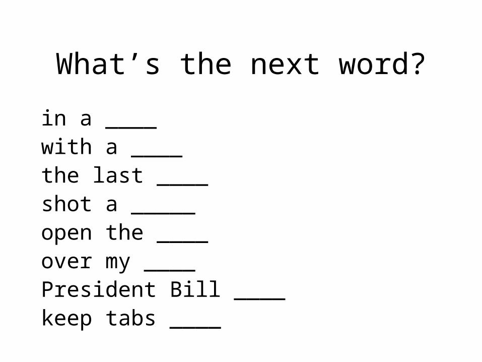
What’s the next word?

in a ____with a ____the last ____shot a _____open the ____over my ____President Bill ____keep tabs ____

borrowed from Henke, based on Manning and Schütze

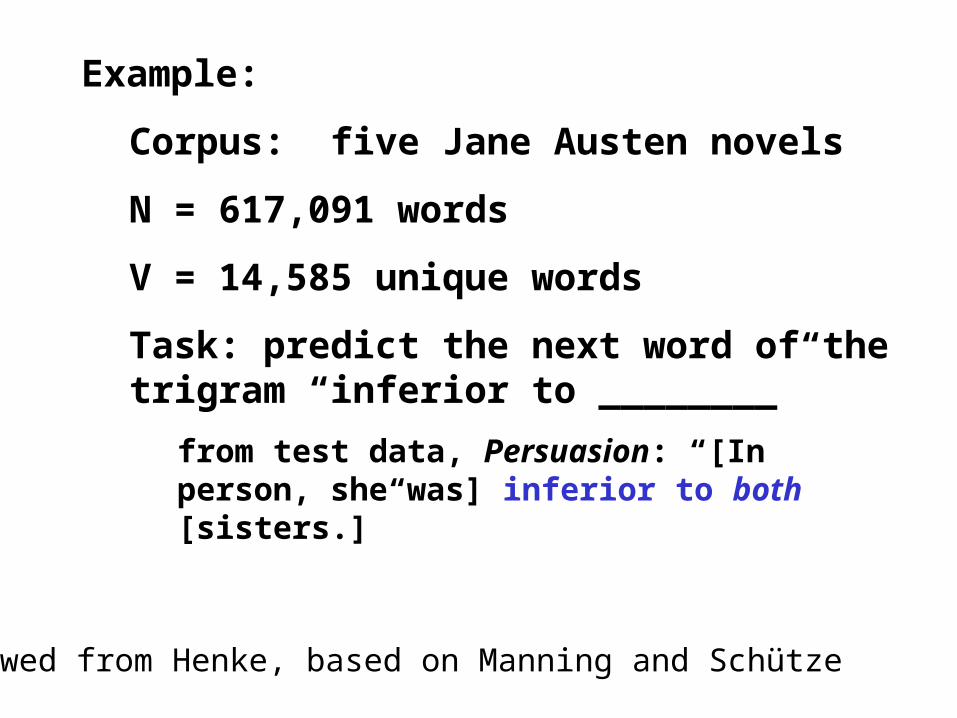
Example:

Corpus: five Jane Austen novels

N = 617,091 words

V = 14,585 unique words

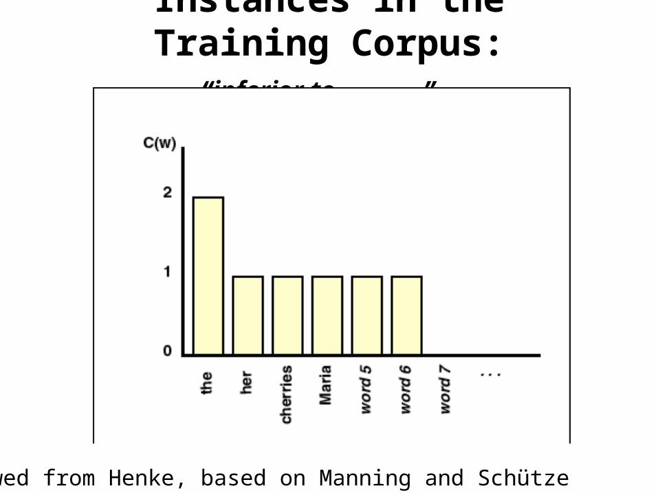
Task: predict the next word of the trigram “inferior to ________”

from test data, Persuasion: “[In person, she was] inferior to both [sisters.]”

borrowed from Henke, based on Manning and Schütze

Instances in the Training Corpus:“inferior to ________”

Maximum Likelihood Estimate:

borrowed from Henke, based on Manning and Schütze

Maximum Likelihood Distribution = DML

• probability is assigned exactly based on the n-gram count in the training corpus.

• Anything not found in the training corpus gets probability 0.

borrowed from Henke, based on Manning and Schütze

Actual Probability Distribution:

Conundrum

• Do we stick very tight to the “Maximum Likelihood” model, assigning zero probability to sequences not seen in the training corpus?

• Answer: we simply cannot; the results are just too bad.

Smoothing

• We need, therefore, some “smoothing” procedure

• which adds some of the probability mass to unseen n-grams

• and must therefore take away some of the probability mass from observed n-grams

Discounting, back-off, and deleted interpolation

• These words all go with “smoothing”.

• “Smoothing” describes the general problem we face: getting probability mass to the great unseen.

• “Discounting” describes who we take probability mass away from, and how much….

• “Back-off” and “deleted interpolation” are the two standard ways of redistributing the probability mass taken away by discounting.

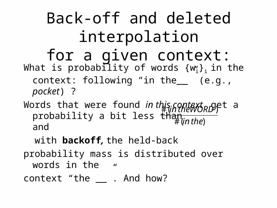
Back-off and deleted interpolationfor a given context:

What is probability of words {wi}i in the context: following “in the__” (e.g., pocket) ?

Words that were found in this context get a probability a bit less thanand

with backoff, the held-back

probability mass is distributed over words in the

context “the __”. And how?

)(#

)(#

thein

WORDthein

Probability mass is distributed over “the WORD” pretty much in proportion to how often each word appears in the context “the___”. But even there, we hold some of the probability mass, and assign it to all words independent of context.

Deleted Interpolation• Is linear: for any word in context (e.g.,

pocket after in the), we choose three ls and take its probability to be the weighted average of the trigram, bigram, and unigram models:1P(pocket|in the) + 2P(pocket|the) + P(pocket)

• If we fixed the ls, we would only need to insist that they sum to 1.0. But…

We don’t fix them: we allow them to vary, depending on the context (“in the”); we need to do some fancier calculations then (Expectation-Maximization).

General ideas about discounting

Three closely related ideas that are widely used.

“Sum of counts” method of creating a distribution

You can always get a distribution from a set of counts by dividing each count by the total count of the set.

“bins”: name for the different preceding n-grams that we keep track of. Each bin gets a probability, and they must sum to 1.0

Zero knowledge

Suppose we give a count of 1 to every possible bin in our model.

If our model is a bigram model, we give a count of 1 to the V2 conceivable bigrams. (V if unigram, V3 if trigram, etc.)

Admittedly, this model assumes zero knowledge of the language….

We get a distribution for each bin by assigning probability 1/V2 to each bin. Call this distribution DN.

Too much knowledge

• Give each bin exactly the number of counts that it earns from the training corpus.

• If we are making a bigram model, then there are V2 bins, and those bigrams that do not appear in the training corpus get a count of 0.

• We get the Maximum Likelihood distribution by dividing by the total count = N.

Laplace (“Adding one”)

Add the bin counts from the Zero-knowledge case (1 for each bin, V2 of them in bigram case) and the bin counts from the Too-much knowledge (score in training corpus)

• Divide by total number of counts = V2 + N

• Formula: each bin gets probability (Count in corpus + 1) / (V2 + N)

Lidstone’s Law Choose a number , between 0 and 1, for the

count in the NoKnowledge distribution.

Then the count in each bin is Count in corpus +

And we assign probability to it (where the number of bins is V2, because we’re considering a bigram model:

2VN

Count

If = 1 this is Laplace;

If = 0.5, this is Jeffrey-Perks Law

If = 0, this is Maximum Likelihood

Another way to say this…

• We can also think of Laplace as a weighted average of two distributions, the No Knowledge distribution and the MaximumLikelihood distribution…

2. Averaging distributionsRemember this:

If you take weighted averages of distributions of this form:

* distribution D1 + (1- ) * distribution D2

the result is a distribution: all the numbers sum to 1.0

This means that you split the probability mass between the two distributions (in proportion then divide up those smaller portions exactly according to D1 and D2.

“Adding 1” (Laplace)

Is it clear that

oodMaxLikeliheNoKnowledg DNV

ND

NV

V

22

2

?122

2

NV

N

NV

V

this is a special case of

DN + (1- )DML

where V2/(V2+N).

How big is this? if V= 50,000, then

V2 = 2,500,000,000. This means that if our corpus is 2 and a half billion words, we are still reserving half of our probability mass for zero knowledge – that’s too much.

= V2/(V2+N) = 2,500,000,000/5,000,000,000 = 0.5

Good-Turing discounting

• The central problem is assigning probability mass to unseen examples, especially unseen bigrams (or trigrams), based on known vocabulary.

• Good-Turing estimation says that a good estimate for the total probability of unseen n-grams is the total number of 1-grams seen = N1/N.

Intuition behind Turing’s idea

• Suppose you want to know, in general, the likelihood that the next word you see will be a word of frequency N, as far as the corpus that you’ve observed so far is concerned.

• Consider the inverted problem: you’ve seen a corpus so far, with a bunch of words with various frequencies….

• We usually think of creating of a corpus as being like consecutive selection of words from a dictionary, with a (stationary) word probability distribution.

• Suppose, instead, that corpus creation consists of: First, selection of a (multi-)set of N words in an unordered fashion; and thenSecond, an ordering is imposed on them by consecutively picking words to be the last word, second-to-last word, etc.:

First:

• Put N words (some different, some the same) in a bag. They’re an unordered set (multiset, really).

Now

• Select what will be the last word of the corpus: Pick it out, label it word #N.

• The bag now has N-1 words in it.

end[N]

Continue: Take out a word, declare it to be word #N-1. Repeat till you get to the first word…

We now have a sequence of moments that illustrate the creation of the corpus (though we did it backwards in time). At each moment, we know what words were in the bag, and we know what word just got removed from it (or rather, what word is just about to be removed from it, from the point of view of normal time)…

Now, back to thinking about Good-Turing from the normal, usual point of view…

• Thinking forward, you want to create a corpus which is one word smaller, so you randomly delete a word from your corpus.

• What’s the probability that you (randomly) choose a word of frequency 1? 2? 27?

• Let’s say there are N1 words of frequency 1, N2 words of frequency 2, etc. Then:i i x Ni = total length of corpus = N, and the probability of removing a word of frequency i is

N

Ni i*

• So the probability of choosing a word that occurred once is N1/N – that is, the number of words that occurred once, divided by the total length of the corpus.

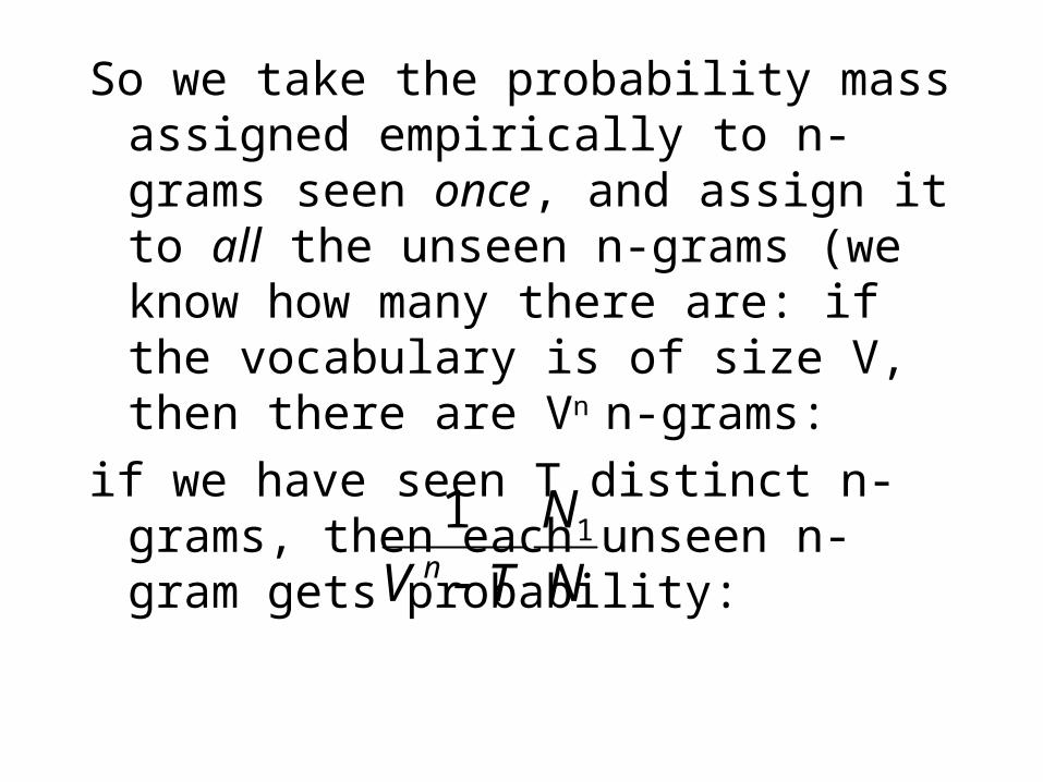
So we take the probability mass assigned empirically to n-grams seen once, and assign it to all the unseen n-grams (we know how many there are: if the vocabulary is of size V, then there are Vn n-grams:

if we have seen T distinct n-grams, then each unseen n-gram gets probability:

N

N

TV n11

• So unseen n-grams got all of the probability mass that had been earned by the n-grams seen once. So the n-grams seen once will grab all of the probability mass earned by n-grams seen twice, then (uniformly) distributed:

N

N

N2

1

1

So n-grams seen twice will take all the probability mass earned by n-grams seen three times…and we stop this foolishness around the time when observed frequencies are reliable, around 10 times.

seen 1x seen 2x 3x 4x 5x

pred 1x pred 2x 3x 4x 5x

MODEL: assigns probabilities

Counts

all unseen ngrams

The End

(if we ignore Bell-Witten)

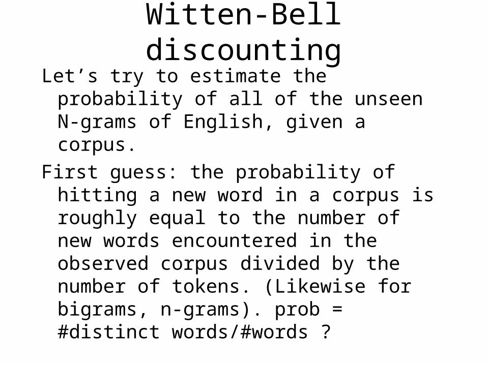
Witten-Bell discounting

Let’s try to estimate the probability of all of the unseen N-grams of English, given a corpus.

First guess: the probability of hitting a new word in a corpus is roughly equal to the number of new words encountered in the observed corpus divided by the number of tokens. (Likewise for bigrams, n-grams). prob = #distinct words/#words ?

That over-estimates…because at the beginning, almost every word looks

new and unseen!

So we must either decrease the numerator or increase the denominator.

Witten-Bell: Suppose we have a data-structure keeping track of seen words. As we read a corpus, with each word, we ask: have you seen this before? If it says, No, we say, Add it to your memory (that’s a separate function). The probability of new words is estimated by the proportion of calls to this data-structure which are “Add” functions.

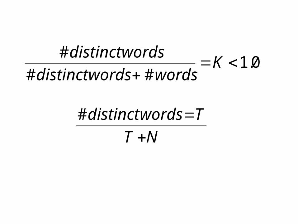
• Estimate prob (unseen word) as

0.1##

#

K

wordswordsdistinct

wordsdistinct

And then distribute K uniformly over unseen unigrams (that’s hard…) or n-grams, and reduce the probability given to seen n-grams

0.1##

#

K

wordswordsdistinct

wordsdistinct

NT

Twordsdistinct

#

• Therefore, the estimated real probability of seeing one of the N-grams we have already seen is N/(T+B), and the estimate of seeing a new N-gram at any moment is T/(T+N).

• So we want to distribute T/(T+N) over the unseen N-grams.