New England Space Science Meeting 2: Transition from the Open to Closed Corona
15
New England Space Science Meeting 2: Transition from the Open to Closed Corona Nathan Schwadron Jan 4, 2005
-
Upload
sylvana-silas -
Category
Documents
-
view
18 -
download
0
description
New England Space Science Meeting 2: Transition from the Open to Closed Corona. Nathan Schwadron Jan 4, 2005. Ideas. Where are the transitions Do we see them with TRACE? Source Surface Models .. Which field lines hae opened during CMEs - PowerPoint PPT Presentation
Transcript of New England Space Science Meeting 2: Transition from the Open to Closed Corona
New England Space Science Meeting 2:
Transition from the Open to Closed Corona
Nathan Schwadron
Jan 4, 2005

Ideas
• Where are the transitions
• Do we see them with TRACE?
• Source Surface Models .. Which field lines hae opened during CMEs
• What is the connection between a region with open field and a region that appears dark in a particular band?

Welcome
• Purpose: – To facilitate interaction among colleagues in space
science in the New England Area (UNH, CfA, BU, MIT, Hanscom/AFRL, Haystack, Dartmouth)
– To leverage these interactions for initiating new, cross-disciplinary and far-reaching projects
• Meetings:– Monthly meetings (first wed each month)– Workshop?

Relationship of open and closed field topologies
• Potential field models (static)• Role of time-dependency (continuous
transitions from open to closed states?)• Conservation of open magnetic flux
– Is open flux conserved, or just preserved
• Highly sectored open fields vs structured closed fields – Open field reflects dipole term– Closed fields on much smaller scales

Relationship of solar wind and coronal heating
• Open field regions free to form steady (supersonic) flows
• Closed field regions injected energy largely lost through radiation
• Is a transition between these regimes expected?

Paths for Deposited Coronal Energy
Injected Electromagnetic
Energy
DownwardConducted Heat,
Radiation,Siphon flows
Bound
, clos
ed
struc
ture
s
Slow wind Fast wind
Open
field
Tra
nsiti
on??
Hot & Bright Cool & DarkIntermediate?Fluctuating?
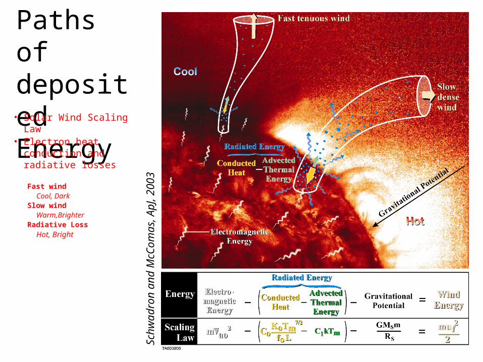
Paths of deposited Energy
Schw
adro
n an
d M
cCom
as, A
pJ, 2
003
• Solar Wind Scaling Law• Electron heat
conduction and radiative losses
Fast windCool, Dark
Slow windWarm,Brighter
Radiative LossHot, Bright

von Steiger et al., JGR, 2000
Background
Well known anti-correlation between solar wind speed and freezing-in temperature, low FIP elements (Geiss et al, Science, 1995; von Steiger et al., JGR, 2000, Gloeckler, et al. 2003)

Constant Energy/particle Source
Schw
adro
n an
d M
cCom
as, A
pJ, 2
003

Flux-Flux Scaling
Constant injected energy/particle implies injected power proportional to particle flux and magnetic flux:
Injected Power proportional to magnetic flux
Injected Elec.Mag. Energy/Particle (assumed constant)
c
4dS 0
E
B Ý N
f 0 d
S 0
B 0 d
S 0

From Solar Wind to X-rays
• Solar wind power
• Yohkoh (2.8-36.6 Å)
Lx~ 1-2% Pcorona ~ 500 0 ??
Psw mu fast
2
2
GM sm
Rs
f1
B1r
0
50,0000 (cgs units)
Solar Wind to X-rays, Lx = 500 0
Pev
stov
et a
l., 2
003,
Sch
wad
ron
et a
l., 2
005
Quiet Sun
X-ray Bright Points
Active Regions
Disk Averages
G,K,M dwarfs
T-Tauri Stars
Solar Wind

X-rays over the
Solar Cycle
Sch
wad
ron
et a
l., 2
005
Power proportional To MagneticFlux

X-rays over the solar cycle
• Solar Wind Power
• GOES (1-8 Å) Active Regions: Lx~ 2.5x10⁻⁴ Pcorona
Quiet Regions: Lx~ 5x10⁻⁵ Pcorona
Coronal Holes: Lx~9x10⁻¹⁰ Pcorona
Psw 50,0000 (cgs units)

McC
omas
et a
l., G
RL
, 200
3
Solar wind’s high degree of organization by speed
Solar Minimum vs Solar Max