The Origins and Implications of MHD Turbulence in Galaxies

Blakesley BurkhartEinstein Fellow

Harvard-Smithsonian Center for Astrophysics

Burkhart, Genel, Pillepich, Hernquist, 2015, in prep. Burkhart & Krumholz, 2015, in prep.

Chepurnov, Burkhart, Lazarian, & Stanimirovic 2015

Outline

• What is turbulence and how to study it in the ISM.

-Origins of Turbulence:• The large scale injection of turbulence energy in

galaxies (kpc driving scales):• Simulations (Illustris) • Observations ( velocity power spectrum of the

SMC in 21cm).

What is turbulence?Inertial range provides: compressibility of the media, dynamic range of the cascade, and comparison with analytical predictions.

Kolmogorov 1941 scaling:E/t~C, t~L/v v~L1/3

E(k)*k~E~v2, k~1/L

E(k)~k-5/3

• Eddies becoming increasingly anisotropic along B with kpara. ~kperp.

2/3 (scale dependent anisotropy; Goldreich & Sridhar 1995, Cho Lazarian 2003 )

(Structure function)

E(k)

E(k)

Phase Coherence

Burkhart et al. 2013a

Burkhart et al. 2014Esquivel & Lazarian 2011

Burkhart & Lazarian in prep.

Burkhart et al. 2010aBurkhart et al. 2009

Tofflemire et al. 2011

Burkhart et al. 2013b, cBurkhart & Lazarian 2012Burkhart Lazarian Gaensler 2012Gaensler et al. 2011Iacobelli et al. 2014

Chepurnov, Burkhart et al. 2014

Burkhart et al. 2013b, cBurkhart Collins Lazarian 2014

The Power Spectrum and Driving of Turbulence

Inertial range provides: compressibility of the media, dynamic range of the cascade, and comparison with analytical predictions.

Where does turbulence come from?

Velocity/density power spectrum reveal multiphase ISM spectra in agreement with expectations for supersonic

turbulenceFor Supersonic Turbulence: density spectrum become shallower and velocity spectrum becomes

steeper (relative to Kolmogorov)

Compare to -5/3=-1.66

Density and velocity power spectrum from Lazarian & Pogosyan (2000, 2004) Velocity Coordinate Analysis (VCA) method.

From Burkhart et al. 2013

Observations of driving scale in multiphase ISM suggest driving on scales larger than clouds (L > 1pc-10pc).

Electron density (WIM) power spectrum:

Larson 1981, Heyer et al. 2009

Molecular medium (line width-size)

WNM/CNM High Lat. Clouds (Chepurnov et al. 2010), VCS

Origins of Turbulence: Multiple Drivers

10 pc-sub-pc scales: Winds, outflows, stellar feedback, stellar wakes

100 Pc scales: supernova, expanding shells, MRI, cloud collisions

1000 Pc scales: Galaxy mergers (major/minor),Expanding shells, Gravitational instability

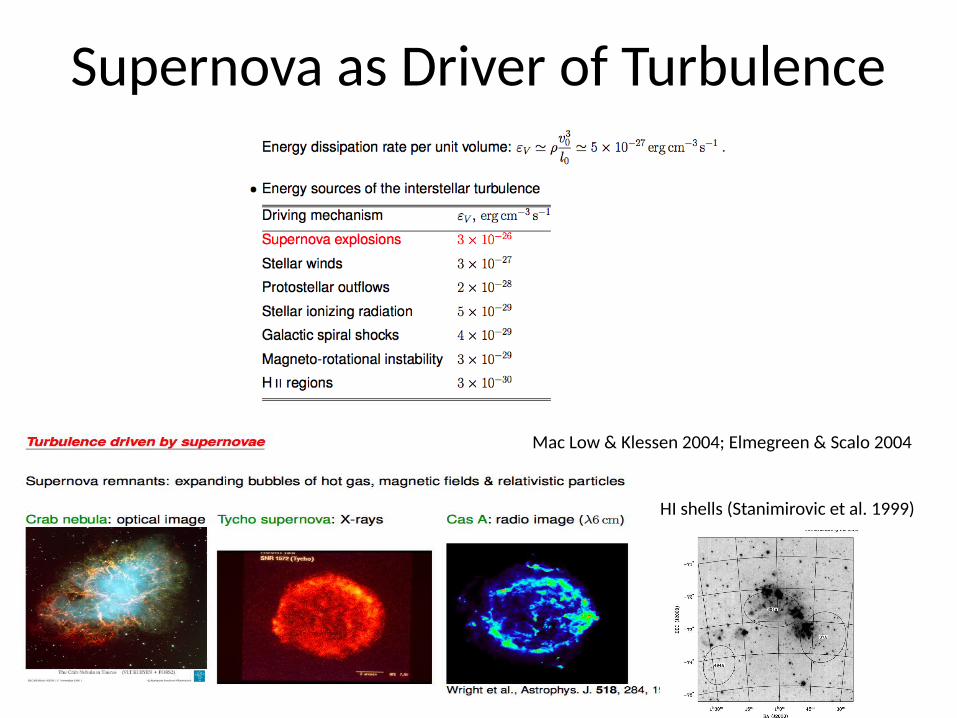
Supernova as Driver of Turbulence

Mac Low & Klessen 2004; Elmegreen & Scalo 2004

HI shells (Stanimirovic et al. 1999)

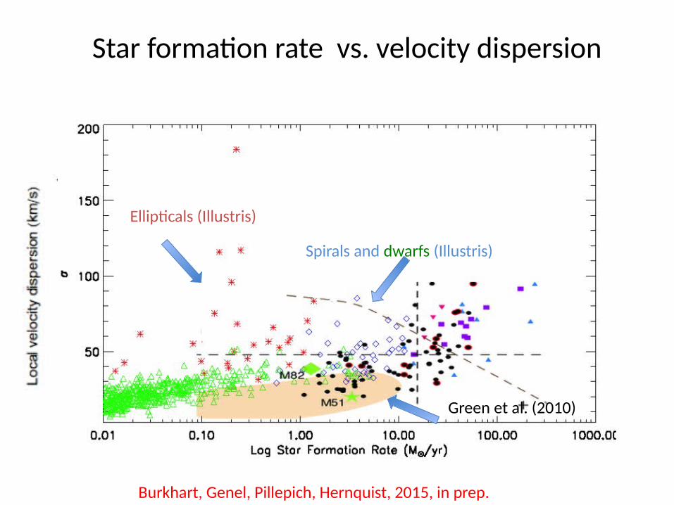
Green et al. 2010Epinat et al. 08,09, 10Law et al. 2009Lemoine-Busserolee et al. 2010

~2.3 kpc resolution

The hundreds of papers question? Do Supernova/Feedback Drive Turbulence at Kpc Scales?

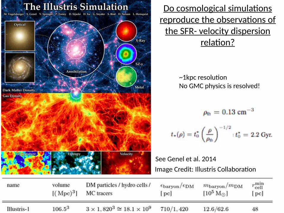
Do cosmological simulations reproduce the observations of

the SFR- velocity dispersion relation?

Image Credit: Illustris Collaboration

~1kpc resolutionNo GMC physics is resolved!

See Genel et al. 2014

Burkhart, Genel, Pillepich, Hernquist, 2015, in prep.

Ellipticals (Illustris)

Spirals and dwarfs (Illustris)

Green et al. (2010)

Star formation rate vs. velocity dispersion

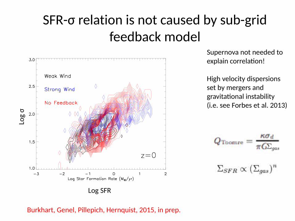
SFR-σ relation is not caused by sub-grid feedback model

Burkhart, Genel, Pillepich, Hernquist, 2015, in prep.

Supernova not needed to explain correlation!

High velocity dispersionsset by mergers and gravitational instability(i.e. see Forbes et al. 2013)

Log SFR

Log

σ

Can Mergers Drive Turbulence?

Panels show stellar light (left) and gas density (right) in a region of 1 Mpc on a side.

Movie Credit: Illustris Collaboration

Mergers can also inject turbulence at kpc scales

Illustris Simulation

Burkhart, Genel, Pillepich, Hernquist, 2015, in prep.

Is there observational evidence for merger induced driving of turbulence?

(Structure function)

E(k)

E(k)

Phase Coherence

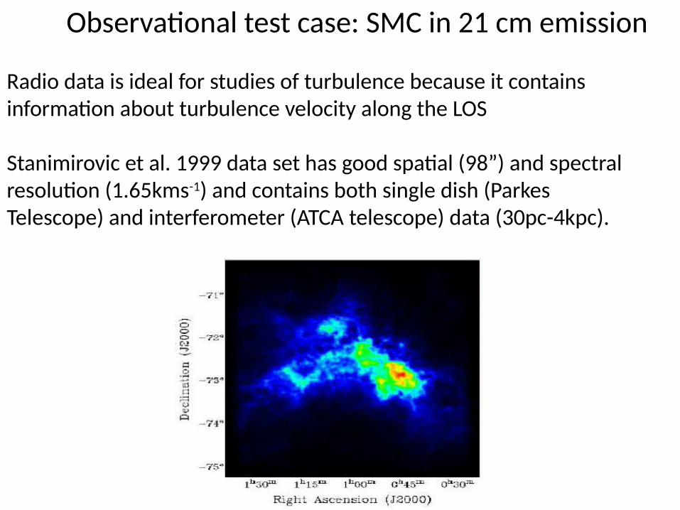
Observational test case: SMC in 21 cm emission

Radio data is ideal for studies of turbulence because it contains information about turbulence velocity along the LOS

Stanimirovic et al. 1999 data set has good spatial (98”) and spectral resolution (1.65kms-1) and contains both single dish (Parkes Telescope) and interferometer (ATCA telescope) data (30pc-4kpc).

VCS of SMC (21cm)Chepurnov, Burkhart, Lazarian & Stanimirovic 2015

Q: What drives turbulence in the SMC? A: Combination of both SF and Mergers!

HI Supershells seen on kpc sizes!

LMC/SMC most likely have already interacted: Tidal stripping of SMC

Stanimirovic et al. 1999

Besla et al. 2012

Chepurnov, Burkhart, Lazarian & Stanimirovic 2015

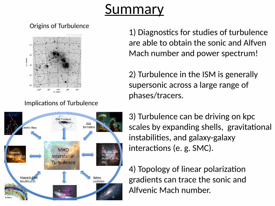
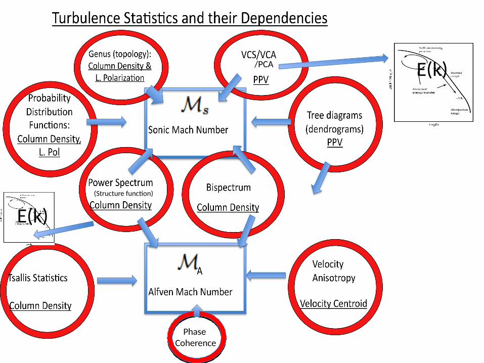
Summary1) Diagnostics for studies of turbulence are able to obtain the sonic and Alfven Mach number and power spectrum!

2) Turbulence in the ISM is generally supersonic across a large range of phases/tracers.

3) Turbulence can be driven on kpc scales by expanding shells, gravitational instabilities, and galaxy-galaxy interactions (e. g. SMC).

Implications of Turbulence

Origins of Turbulence

Interested in turbulence diagnostics for your observations/simulations?

Come talk to me!

Burkhart & Krumholz 2015 in prep.

High velocity dispersions can be set by gravitational instability: consider the Toomre instability.

Q>1, stable rotating disk

Given a driving scale of 1kpc and turbulent amplitude of V=50 km/s.This is comparable to the eta from fiducial numbers of supernova driving of 3x10-26 ergs/s cm^-3 (i.e. see Mckee Klessen 2004) and the turbulence dissipation rate (3x10-27 ergs/s cm^-3).

Turbulence & Polarization Maps: 1.4 Ghz Southern Galactic Plane Survey (SGPS)

Gaensler et al. 2001

Question: What are these filamentary structures seen in Stokes P but not total intensity?

ATCA interferometer

Linear polarization gradients Turbulence

Structures are due to Faraday Rotation along LOS…

Sharp changes in or B along the LOS can be due to random (subsonic) fluctuations and/or shocks propagating through the ISM

can be related to more theoretically motivated

Characterize sharp changes with polarization gradients.

ATCA interferometer:1.4 Ghz Southern Galactic Plane Survey

Gaensler +01

Gradients of Polarization Data: Simulations and Statistics

Subsonic Supersonic

Filaments due to supersonic and subsonic turbulence are different in:1) Topology2) PDFs

(Gaensler et al. 2011 Nature and Burkhart, Lazarian & Gaensler 2012 ApJ)

Post process simulations to linear polarization with external Faraday rotation

Gradients of Turbulent Fields: Topology

Example:Any fractal function…All turbulence!

Example:Strong fluctuations, weak shocks…transsonic turbulence

Example:Strong interacting Shocks…high Mach number!

Burkhart, Lazarian & Gaensler 2012

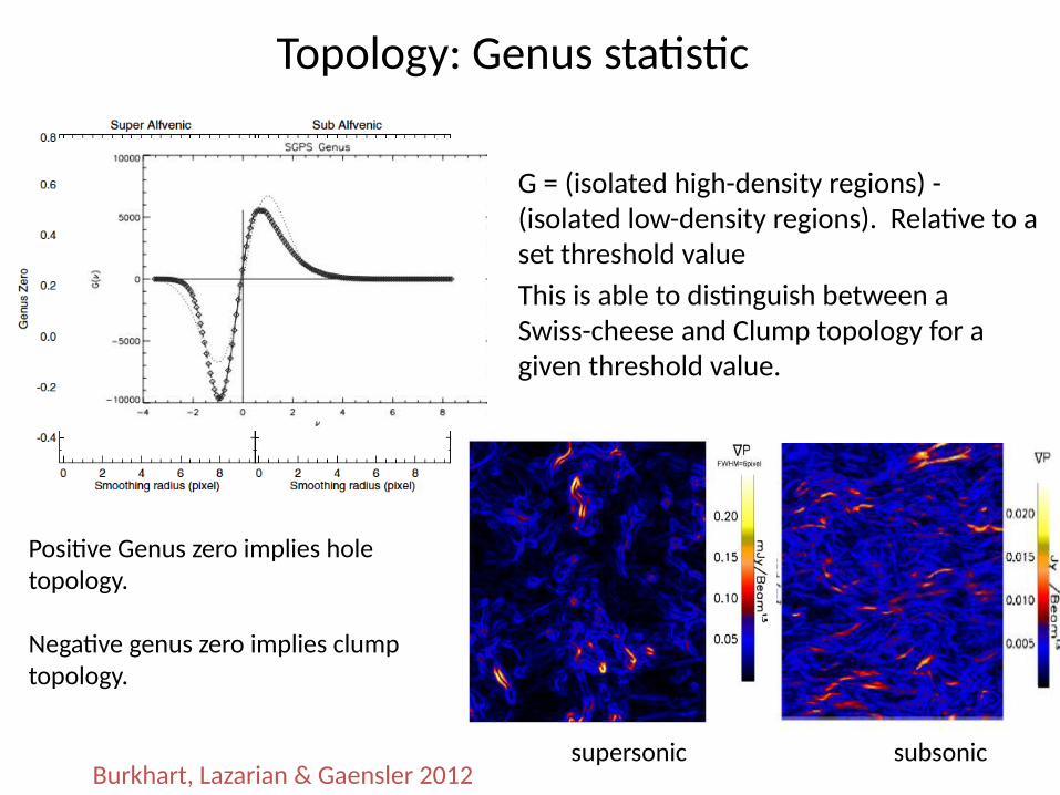
Topology: Genus statistic

G = (isolated high-density regions) - (isolated low-density regions). Relative to a set threshold value

• This is able to distinguish between a Swiss-cheese and Clump topology for a given threshold value.

Positive Genus zero implies hole topology.

Negative genus zero implies clump topology.

Burkhart, Lazarian & Gaensler 2012supersonic subsonic

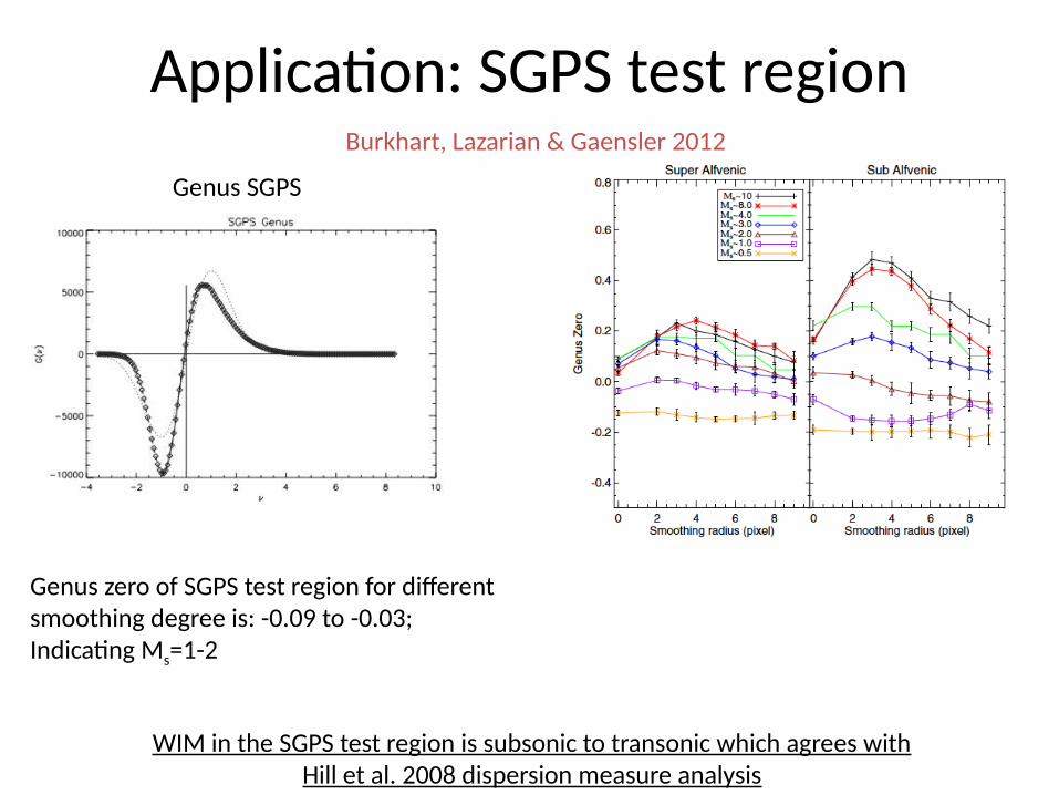
Application: SGPS test region

Genus zero of SGPS test region for different smoothing degree is: -0.09 to -0.03; Indicating Ms=1-2

Genus SGPS

WIM in the SGPS test region is subsonic to transonic which agrees withHill et al. 2008 dispersion measure analysis

Burkhart, Lazarian & Gaensler 2012

Summary1) Diagnostics for studies of turbulence are able to obtain the sonic and Alfven Mach number and power spectrum!

2) Turbulence in the ISM is generally supersonic across a large range of phases/tracers.

3) Turbulence can be driving on kpc scales by expanding shells, gravitational instabilities, and galaxy-galaxy interactions (e. g. SMC).

4) Topology of linear polarization gradients can trace the sonic and Alfvenic Mach number.

Implications of Turbulence

Origins of Turbulence

Can Mergers Drive Turbulence?

Panels show stellar light (left) and gas density (right) in a region of 1 Mpc on a side.

Movie Credit: Illustris Collaboration

Origins of Turbulence: Multiple Drivers

10 pc-sub-pc scales: Winds, outflows, stellar feedback, stellar wakes

100 Pc scales: supernova, expanding shells, MRI, cloud collisions

1000 Pc scales: Galaxy mergers (major/minor),Expanding shells, Gravitational instability

(Structure function)

E(k)

E(k)

Phase Coherence

/PCA

Phase Coherence

Bispectrum

Column Density

Column Density

Esquivel & Lazarian 2011Burkhart et al. 2014 Tofflemire Burkhart Lazarian 2012

Burkhart & Lazarian 2015

Burkhart & Lazarian 2015 Burkhart et al. 2010Burkhart et al. 2009

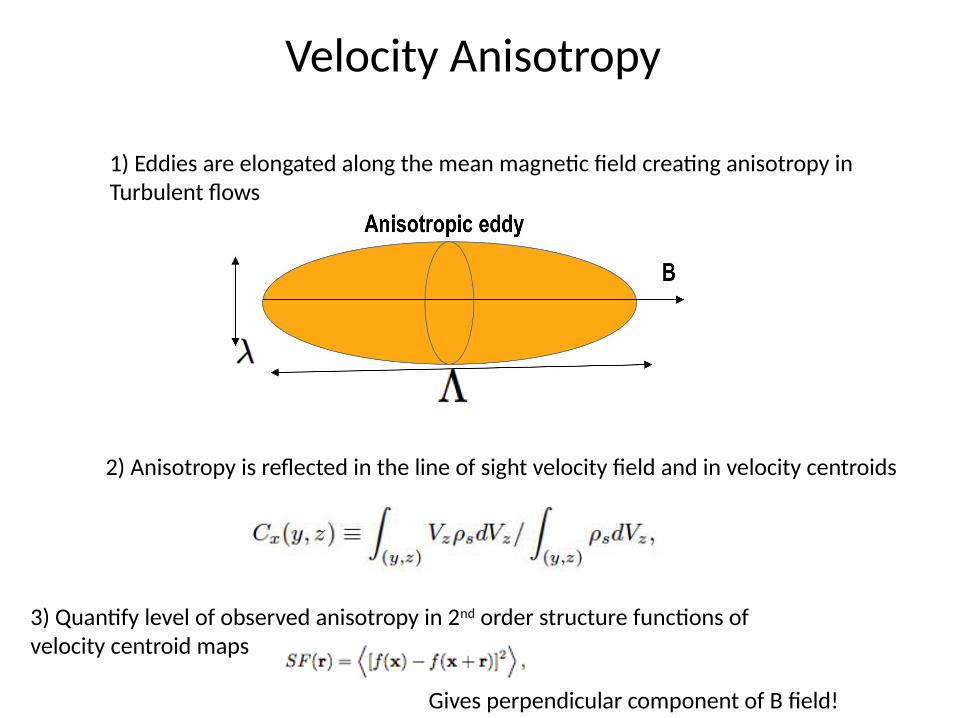
Velocity Anisotropy

1) Eddies are elongated along the mean magnetic field creating anisotropy in Turbulent flows

2) Anisotropy is reflected in the line of sight velocity field and in velocity centroids

3) Quantify level of observed anisotropy in 2nd order structure functions of velocity centroid maps

Gives perpendicular component of B field!

Velocity CentroidsEsquivel & Lazarian11Burkhart et al. 2014

1) Implies B-perp can be obtained via statistics2) Little dependency on sonic Mach number3) Complimentary to PCA anisotropy methods (Heyer et al 2008)

PDFs of Column Density-Ms

2nd moment: Variance (σ2 linear and log PDF) vs. Ms

3rd moment: Skewness(linear PDF) vs. Ms

4th moment: Kurtosis(linear PDF) vs. Ms

Ms=0.5 Ms=2.0 Ms=4.5 Ms=8.0

Skewness=A*Ms+b

Kurtosis=A*Ms+b

Linear Column Density PDF

Ms=0.5Ms=2.0Ms=8.0Ms=4.5

Column density PDFs:Kowal et al. 07; Burkhart et al. 09,10; Burkhart & Lazarian 12; Kainulainen & Tan 13

MHD Simulations (no gravity)-Cho et al. 2003, ENZO (Collins et al.) codes

-Solve the ideal MHD equations in a periodic box and assume an isothermal equation of state P=cs

2p.

-Generate 3D simulation with resolution 5123

Ms=v/cs= 0.7,2.0,4.5,7.0,8.0, 10MA=v/vA= 0.7,2.0

Similar to many other MHD ‘turbulence in box’ simulations

s

B|| B

Kowal Lazarian 2007 Ms=7. MA=0.7

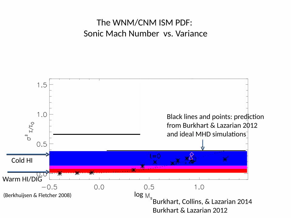
The WNM/CNM ISM PDF: Sonic Mach Number vs. Variance

Cold HI

Warm HI/DIG

IRDCs (Kainulainen & Tan 2013)

ENZO self-gravitating

Burkhart, Collins, & Lazarian 2014Burkhart & Lazarian 2012

(Berkhuijsen & Fletcher 2008) log

Black lines and points: prediction from Burkhart & Lazarian 2012 and ideal MHD simulations

PDFs of Collapsing GMCs are Different than WNM/CNM….

Collins et al. 2012; Burkhart, Collins, Lazarian 2014, submitted

t=0 supersonic turbulencet>0 re-run with ENZO AMR self-gravity

Movies: D. Collins

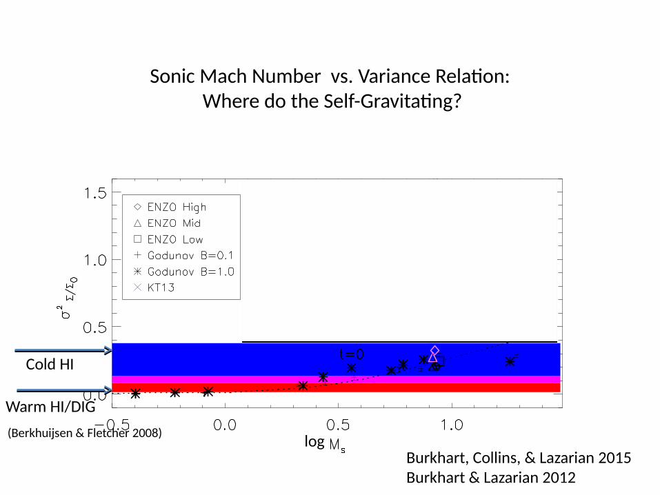
Sonic Mach Number vs. Variance Relation: Where do the Self-Gravitating?

Cold HI

Warm HI/DIG

IRDCs (Kainulainen & Tan 2013)

ENZO self-gravitating

Burkhart, Collins, & Lazarian 2015Burkhart & Lazarian 2012

(Berkhuijsen & Fletcher 2008) log

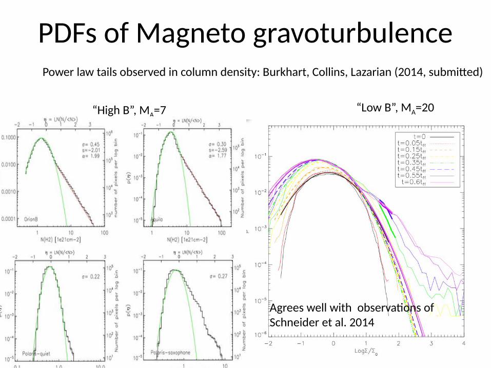
PDFs of Magneto gravoturbulence

“High B”, MA=7 “Low B”, MA=20

Power law tails observed in column density: Burkhart, Collins, Lazarian (2014, submitted)

Agrees well with observations ofSchneider et al. 2014

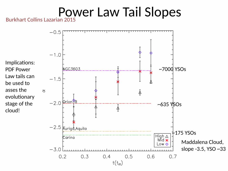
Power Law Tail Slopes

~7000 YSOs

~175 YSOs

Maddalena Cloud, slope -3.5, YSO ~33

~635 YSOs

Implications: PDF Power Law tails can be used to asses the evolutionary stage of the cloud!

Burkhart Collins Lazarian 2015

Conclusions

1) The PDF can diagnose the turbulent state of the gas (sonic Mach number) for the diffuse medium.

2) For self-gravitating gas the PDF is a better indicator of the evolutionary stage of the cloud.

3) Orion B seems to be in an intermediate state of evolution compared with other clouds (as traced by the PDF).

4) Additional tracers for PDFs beyond dust are need to to get the full dynamic range of the PDF in molecular clouds, i.e. to probe the ‘lognormal’ portion (Lombardi, Alves & Lada 2015).