1

NEUROECONOMICS, ILLUSTRATED BY THE STUDY OF AMBIGUITY-AVERSION

COLIN F. CAMERER MEGHANA BHATT

MING HSU DIV HSS 228-77, CALTECH, PASADENA CA

This paper is about the emerging field of neuroeconomics, which seeks to ground economic

theory in details about how the brain works. This approach is a sharp turn in economic thought. Around

the turn of the century, economists made a clear methodological choice, to treat the mind as a black box

and ignore its details for the purpose of economic theory (13). In an 1897 letter Pareto wrote

It is an empirical fact that the natural sciences have progressed only when they have taken secondary principles as their point of departure, instead of trying to discover the essence of things. ... Pure political economy has therefore a great interest in relying as little as possible on the domain of psychology (quoted in Busino, 1964, p. xxiv (14)). Pareto’s view that psychology should be ignored was reflective of a pessimism of his time, about

the ability to ever understand the brain.1 As William Jevons wrote a little earlier, in 1871

I hesitate to say that men will ever have the means of measuring directly the feelings of the human heart.

It is from the quantitative effects of the feelings that we must estimate their comparative amounts (45).

This pessimism about understanding the brain led to the popularity of “as if” rational choice models.

Models of this sort posit individual behavior which is consistent with logical principles, but do not put

any evidentiary weight on direct tests of whether those principles are followed. For example, a consumer

might act as if she attaches numerical utilities to bundles of goods and choose the bundle with the highest

utility, but if you ask her to assign numbers directly her expressed utilities may not obey axioms like

transitivity. The strong form of the as-if approach simply dismisses such direct evidence as irrelevant

because predictions can be right even if the assumptions they are based on are wrong (e.g., Friedman,

1953 (36)).2

As-if models work well in many respects. But tests of the predictions that follow from as-if

rational choice (as well as direct tests of axioms) have also established many empirical anomalies.

Behavioral economics describes these regularities and suggests formal models to explain them (e.g.

Camerer, 2005). Debates between rational-choice and behavioral models usually revolve around 1 However, Colander (2005)(23; 20) notes that Ramsey, Edgeworth and Fisher all speculated about measuring utility directly before the neoclassical revolution declared utility to be inherently unobservable and only revealed by observable choices. Ramsey and Edgeworth speculated about a ”psychogalvanometer” and a ”hedonimeter”, respectively, which sound remarkably like modern tools. Would these economists be neuroeconomists if they were reincarnated today? 2 The most charitable way to interpret Friedman’s “F-twist” is that theories of market equilibrium based on utility-maximization of consumers are equivalent, at the market level, to unspecified other theories which allow violations of utility-maximization but include some institutional repairs or corrections for those violations. That is, the theory states U M , but even if U is false, there is an alternative theory [(not - U)andR] M, in which a “repair condition” R suffices in place of assumption U, to yield the same prediction M. If so, the focus of attention should be on specifying the repair condition R.

2

psychological constructs, such as loss-aversion (46) and a preference for immediate rewards, which have

not been observed directly. But technology now allows us to open the black box of the mind and observe

brain activity directly. The use of data like these to constrain and inspire economic theories, and make

sense of empirical anomalies, is called “neuroeconomics” (17; 22; 73). It is important to note that

neuroeconomists fully appreciate that the revealed-preference approach does not endorse the idea of

measuring utilities directly (44). The neuroeconomic view does not “misunderstand” the revealed

preference approach to economics; it simply takes a different approach. Furthermore, the presumption is

that creating more realistic assumptions will lead to better predictions. Friedman’s view was that (1)

theories should be judged by accuracy of predictions; and (2) false assumptions could lead to accurate

predictions. Neuroeconomics shares the emphasis on accuracy in principle (1), but also bets on the

possibility that improving the accuracy of assumptions will lead to more accurate predictions.

An analogy to organizational economics illustrates the potential of neuroeconomics. Until the

1970’s, the “theory of the firm” was basically a reduced-form model of how capital and labor are

combined to create a production function, as the basis for an industry supply curve. Contract theory

opened up the black-box of the firm and modeled the details of the nexus of contracts between

shareholders, workers and managers (which is what a firm is). The new theory of the firm replaces the

(still useful) fiction of a profit-maximizing firm which has a single goal, with a more detailed account of

how components of the firm interact and communicate to determine firm behavior. Neuroeconomics

proposes to do the same by treating an agent like a firm: Replace the (useful) fiction of a utility-

maximizing agent who has a single goal, with a more detailed account of how components of the agent’s

brain interact and communicate to determine agent behavior.

Much of the potential of neuroeconomics comes from recent improvements in technology for

measuring brain activity. For example, fMRI measures oxygenated blood flow in the brain (which is

correlated with neural activity on the scale of a couple of seconds and a few millimeters). Behavior of

animals and patients with localized lesions to specific areas of the brain can help us determine if the

damaged area is necessary for certain behaviors. At an even more detailed level, one can record activity in

a single neuron at a time (single-unit recording), generally from primates but occasionally from

neurosurgical patients. Older tools like electroencephalogram (EEG), recording very rapid electrical

activity from outer brain areas, and psychophysiological recording (skin conductance and pupil dilation,

for example), continue to be useful, often as complements that corroborate interpretations from other

methods.

All these tools give clues about a detailed theory of how decision making actually works. The

success of the rational actor model in “as if” applications shows that this level of detail is not necessary

for certain sorts of analysis, especially those that deal with populations of decision makers instead of

3

individuals. (For example, neuroeconomics will never displace the powerful concepts of supply and

demand, and market equilibrium.) However, a deeper understanding of the mechanics of decision making

will help us understand deviations from the rational model better. Knowing the process of decision

making should allow us to understand not only the limits of our abilities to calculate optimal decisions,

but also the heuristics that we use to overcome these limits.

Furthermore, in most areas of behavioral economics there is more than one alternative theory.

Often there are many theories which are conceptually different but difficult to separate with current data.

To the extent that some of these theories commit to neural interpretations, the brain evidence can help sort

out which theories are on the right track and also suggest new theories. The study of “ambiguity-

aversion” detailed in section 4 is intended in this paper as a case study how two types of brain evidence

(fMRI and lesion-patient behavior) can adjudicate a long-standing debate in decision theory about

whether ambiguity-aversion exists and where it comes from.

The ability to use these neuroscientific technologies to establish neural circuitry depends on the

fact that the brain is largely modular in structure. A lot is known about which general areas of the brain

deal with vision, hearing, and other sensory information; and these areas are consistently activated across

people. While the degree of modular specialization is sometimes surprising (e.g., there is a “facial

fusiform area” apparently devoted to face recognition), most higher-order processing requires a “circuit”

or collaboration among many component processes which are in turn parts of different modules. Less is

known about higher processing than specific sensory processing, but neuroscientists have a general idea

of where certain types of emotional and rational processing occurs, and empirical regularity is

accumulating very rapidly.

1. NEUROECONOMIC BRAIN IMAGING EXPERIMENTS

Brain imaging, or scanning, is the neuroscientific tool that now gets the most attention. Functional (fMRI)

imaging uses the same magnetic resonance (MR) scanner that has been used for medical purposes for

decades. The innovation in fMRI, which began only about ten years ago, is scanning the brain much more

rapidly to detect differing levels of oxygenated blood in the brain when subjects are performing some

task. Most brain imaging involves a comparison of brain activity when a subject performs an an

“experimental” task and a “control” task. The difference between images taken while the subject is

performing the two tasks provides a picture of regions of the brain that are differentially activated by the

experimental task. The modular nature of the brain allows us to interpret these activations in the context

of other evidence about what tasks activate the same areas.

Imaging is increasingly popular for two reasons. First, it is non-invasive, unlike single neuron

recording, which implants electrodes directly into the brain, or transcranial magnetic stimulation (TMS),

4

which stimulates brain areas creating temporary lesions. Second, fMRI provides relatively good temporal

and spatial resolution, even for areas deep in the brain (which cannot be measured by EEG). Images are

taken every few seconds and data are recorded from voxels which are 3-4 cubic millimeters in size.

Scanning is expensive, but usually modest sample sizes (10-20 subjects) are enough to establish

suggestive regularity if studies are well-designed.

There have already been several prominent studies of economic decision making using fMRI and

PET (Positron Emission Tomography), another form of scanning technology3. We mention a few to show

how imaging can address the kinds of questions economists care about. All these results are tentative;

more will be learned rapidly in the next few years.

1.1. Game theory and social emotions. Experiments have proved very useful in testing game theory,

because game theory often depends on subtle details of moves and information which can be easily

controlled in an experiment (and difficult to measure in many field applications (19)). Neuroeconomics

experiments enable a similar attention to detail of how equilibration results from cognition and how social

preferences influence strategic behavior.

In an early study, McCabe et al (2001)(53) compared brain activity when subjects played trust

games against other humans, compared to playing against randomized opponents. Among players who

did not cooperate very often, there were no differences in activity between the two conditions. But among

high cooperators, there was additional activity in frontal cortex when playing other humans. McCabe et al

interpret this activity as evidence of a specialized “theory of mind” circuitry used to form beliefs about

what other human players will do. Frith et al find a similar result comparing play of a mixed-strategy

game (rock, paper, scissors) against a randomized opponent that the subject was told was a computer to a

randomized opponent that the subject was told was human. In both cases subjects were simply playing

against the Nash equilibrium strategy that randomizes between all three strategies, but in the condition

where they were told they were playing another human being there were significant activations in the

anterior paracingulate cortex (39). These studies show neurally, that forming beliefs about another

player’s moves is fundamentally different then forming beliefs about “nature’s” moves, even when these

are empirically identical.

In the ultimatum game, one player, the proposer, offers a take-it-or-leave-it share x of an amount,

say $10, to another player, the responder. If the responder takes the offer they both earn $10-x and x,

3 For PET, subjects are injected with a small amount of radioactive solution (often glucose with a radioactive marker) and the scanner simply localizes where the radioactive material goes during different tasks. The advantage of this method over fMRI is that PET measures glucose metabolism, a more direct correlate to neural activity than the BOLD signal. The major disadvantage is that it has a much lower temporal resolution (on the order of minutes rather than seconds)

5

respectively. If the responder rejects the offer they both get nothing and the game is over. This game has

been studied in hundreds of experiments. The typical result is that players offer around 40% of the pie

(often half), and offers below 20% are rejected in most societies (e.g. (19) chapter 2).4

Sanfey et al (63) studied the behavior of responders who received offers in ultimatum games,

using fMRI. They found that when offers were unfair ($1-2 out of $10) compared to fair, three areas were

active: Dorsolateral prefrontal cortex (DLPFC), anterior cingulate (ACC) and insula. The insula is an area

that is active in registering body discomfort; it is activated when people feel, among other things, social

exclusion (31), and disgust (15). Their interpretation is that neurons in the insula are activated by

unfairness, the DLPFC is processing future reward from keeping the money, and the ACC is an arbiter

that weighs these two conflicting inputs to make a decision. Whether players reject unfair offers or not

can be predicted rather reliably (a correlation of .45) by the level of their insula activity.

One controversy in behavioral economics is the nature of social preferences expressed in games

like the ultimatum game, trust games, and their kin which are used to study reciprocity. Consider

punishment, the willingness of A to punish B, if A believes B has treated her badly. If the players play

only once, A has no direct or reputational incentive to punish B at all. So what is A thinking or feeling

when she punishes B?

This question was studied using PET imaging by de Quervain et al (26). In their study, two

players, A and B, played a trust game in which A invested money, which grew in value, and the “trustee”

player B could repay or keep the money(71; 9). The subject, A, whose behavior was imaged was asked,

after play, whether she wanted to punish the trustee or not. The “price” of punishment was also varied so

that during some conditions A punished at a direct cost to herself.

When players punished, de Quervain et al found activity in the nucleus accumbens (part of the

striatum), a region known for processing rewards derived from actions (58). Thus, punishment appears to

generate an internal sense of reward, just as receiving money does. They also found activity in frontal

cortex when the price of punishment was being weighted. To an economist, this means that a preference-

based theory in which punishment motives and money-earning motives are neurally similar, and respond

to prices in a thoughtful way implemented by frontal cortical activity, ts what the brain is doing and

provide a simple way to modify the self-interest assumption mathematically.

fMRI has also been used to help understand the neural basis of the concept of equilibrium in

games. In game theory, players are in equilibrium when they all best-respond to accurate beliefs about

what other players will do. But this concept of equilibrium is focused on a static situation; it says nothing 4 There are interesting variations between average offers across societies, however, which are correlated with the degree of market integration and production of public goods in those societies (Henrich et al, 2003 (19)). From a neural point of view, we believe differing social norms of fairness in these societies probably generate different activity in insula, which generate different offer and rejection patterns. Just as the food and social habits that people find disgusting can vary across cultures, so can norms of what offers are “disgustingly unfair”.

6

about how players reach equilibrium. One neuroscientific hypothesis of equilibrium is that an equilibrium

choice requires that the player use similar circuitry to make her own choice, and form her beliefs about

the other player, perhaps simulating the other player’s choice, to make an accurate guess. Put differently,

if a player is using a simple decision rule like “one-step reasoning” (pick the strategy with the highest

average payoff, as if the other players’ choices are all equally likely), then more reasoning will be evident

calculating the optimal choice than in guessing what others will do (because the guess is a simple diffuse

prior which requires little thought).

These considerations suggest that when activity during the act of making a choice, and activity

when making a guess, overlap sufficiently, equilibrium choices are more likely – that is, equilibrium is a

“state of mind” revealed by a high degree of mental overlap in choosing and guessing. Indeed, Bhatt and

Camerer (12) found a sharp difference between differential activity in choosing and reporting beliefs

when trials were in equilibrium (beliefs were accurate and choices were optimal given guesses) and out-

of-equilibrium.

In equilibrium trials, there is only a small difference in activity between choosing and reporting

beliefs. This difference is in the ventral striatum, an area known to encode anticipated reward. This area

may imply that players expect larger rewards from making choices (since the payment schemes were not

identical across the two tasks of choosing and guessing), or that players have a kind of internal “cash

register” which senses when they have made an accurate equilibrium choice, even though the games were

played without feedback.

In out-of-equilibrium trials, there was differing activity in many areas between the task of

choosing a strategy and to guessing what others will choose. These areas include the DLPFC (observed

by Sanfey et al), and paracingulate cortex (observed by Frith et al). This is consistent with the idea that

many players have a rather shallow way of forming beliefs which requires little processing, consistent

with some behavioral models of limited “levels of thinking” (21).

Bhatt and Camerer also studied what happens when players generate second-order beliefs – that

is, what do they think the other player thinks they will do? (These complex judgments are important in

successful deception and in creating social emotions like shame5). There are two ways to generate a

second-order belief: (1) Apply some general circuitry for forming a belief, but take the other player’s

perspective; or (2) figure out what you plan to choose, and then ask whether the other player is likely to

guess your choice. Two facts support the second explanation: Choices and second-order beliefs match

surprisingly often; and there is more overlap in neural activity during the choice and second-order belief 5 (29) measured second-order beliefs in trust games similar to those studied by McCabe et al above. In their games, each investor was asked how much they thought the trustee would repay (call this guess Einvestor (y)), and the trustee was asked to guess the investor’s guess about repayment (i.e,. Etrustee (Einvestor (y))). The second-order guess was correlated (.44) with the trustee’s actual repayment y. This correlation suggests the trustee’s feel a sense of moral obligation to live up to the investor’s expectations, so their second-order belief about what that investor expectation is, is an important driver of their decision.

7

tasks than between those tasks and the belief task. Furthermore, players who were more self-focused, in

the sense of equating their choice and their second-order belief (differentially activating the anterior

insula) actually earned less in the game.

1.2. Intertemporal choice. The problem of intertemporal choice has been studied at length in economics

and psychology. One apparent empirical fact is that people display a “preference for immediacy”. When

faced with two decisions about future payoffs, one later than the other, they act as if they are very patient

(i.e. they possess a relatively high discount factor). When these same subjects are given the choice

between an immediate reward and a future payoff they show a strong tendency to choose the immediate

reward, implying a much lower discount factor (50; 59). Fitting discount factor functions to data from

rewards at different points in time across many animal species (including humans) generally shows a

hyperbolic form, d(t) =1/(1 + kt), rather than an exponential d(t) = dt. For modeling purposes, a good

approximation to the hyperbolic form is a two-piece “quasi-hyperbolic” function, which weights current

rewards by 1, and future rewards at time t by ßδt(50). When ß =1 the function reduces to an exponential.

The parameter ß captures the preference for immediacy, and δ expresses the relative preference for

rewards at different future points.

This two-piece function is a natural candidate for study in fMRI because the two systems can be

isolated by comparing different types of choices. Indeed, McClure et al find that when people choose

between an immediate reward and a future reward (with presumed weights of 1 and ßδ) relative to two

distant rewards (with relative weights of δt and δt+1) areas with projections from the limbic regions are

active. When weighing any two choices, many areas are active, but only prefrontal and anterior cingulate

areas seem to be involved in the δ system.

2. FINDING CIRCUITRY

Finding areas of differential brain activity from fMRI is not actually the main goal of these

studies. The real goal is to use the observed brain activity to hypothesize a “circuit” of different brain

regions that interact to generate a behavior (such as a decision). To understand the circuit, we need to

know which areas are active, and how they interact. Using scanning evidence, the neural circuitry of

decisions must be largely inferred from what we know of neurophysiology and the time series of

activations in various parts of the brain. Even so, scanning evidence is only sufficient to show that the

activated regions are correlated with the decision task. More evidence is necessary to establish any causal

link between brain areas and decisions.

One way to determine whether a region is a necessary part of a circuit is to observe patients who

have local lesions in that region. These patients are generally victims of strokes, encephalitis, other brain

8

injuries, and neurosurgical interventions. An ideal lesion patient has a localized lesion, preferably bilateral

(on both sides of the brain), which overlaps a specialized functional or neuroanatomical area of the brain.

If the patient with damage to region X is reasonably normal in most cognitive functions (like IQ and

memory), and if the patient does not do a task normally, we can infer that region X is a necessary part of

the circuit for that task. Other methods of establishing necessity include creating temporary lesions using

TMS. But even these techniques only establish that the regions are necessary for a task, not that they are

sufficient. There is also some research being done on the role of different neurotransmitters, rather than

specific brain areas, in certain decision making processes. These studies can actually demonstrate the

sufficiency of different neurotransmitters for certain behaviors. For example Kosfeld et al. found that you

can increased the level of trust in a person by administering a dose of oxytocin.(49).

Lesion patients show startling dissociations between tasks that seem remarkably similar. For

example, there are lesion patients who can write well, but can’t read. Patients with permanent

“anterograde amnesia” – the awful inability to form new memories – do not form conscious declarative

explicit memories for emotions or physical procedures. However, these patients actually do form such

memories implicitly; that is, they know information but don’t know that they know it. This dissociation

indicates that declarative memories, and meta-knowledge are stored separately.6

The study described in the section below uses a combination of fMRI scanning evidence and

behavioral data from lesion patients to examine the circuitry of choice under uncertainty. Lesions in the

same areas activated in a scanning study can help us understand the interactions of the regions and

establish whether a lesioned area is a necessary part of a hypothesized circuit.

Another important tool which will prove valuable in neuroeconomics is what neuroscientists call

“computational models” (which economists would call a “calibration exercise”). In computational

models, a detailed numerical specification of a neural circuit is suggested. Given those details, simulated

input to the circuit leads to a predicted output (typically depending on the values of some free

parameters). The model is calibrated by finding parameter values which maximize the .t of predicted

output to actual data. Compared to models in economics, these specifications are often incredibly detailed

and clearly motivated by what is known about neuroanatomical connections between areas (e.g., Kim and

Whalen (47)). As in economic theory, computational models are valuable because they force the modeler

to be perfectly clear about how the components of a circuit are linked, and the hypothesized circuit is

subjected to empirical scrutiny.

6 For example, if you show anterograde amnesiacs a chess board and ask “Do you know how to play?” they will often say “No” even if they’ve been taught the rules before. But if you force them to play – “Let’s just start” – they will play chess according to the rules. They know the rules, they just don’t know that they know them. This syndrome was illustrated effectively in the popular 2002 movie “Memento”(6).

9

3. AMBIGUITY AVERSION

The study described in this section uses a combination of fMRI scanning evidence and behavioral

experiments with lesion patients to examine the circuitry of choice under uncertainty. It is meant as a

detailed illustration of how fMRI can be used to do neuroeconomics, with more detail than is typically

permitted in neuroscience journals.

In theories of choice under uncertainty used in social sciences and behavioral ecology, the only

variables which should influence an uncertain choice are the judged probabilities of possible outcomes

and the evaluation of those outcomes. But confidence in judged probability can vary widely. In some

choices, such as gambling on a roulette wheel, probability can be confidently judged from relative

frequencies, event histories, or from an accepted theory. At the other extreme, such as the chance of a

terrorist attack, probabilities are based on meager or conflicting evidence, where important information is

clearly missing. The two types of uncertain events are often called risky and ambiguous, respectively. In

subjective expected utility theory (SEU), the probabilities of outcomes should influence choices but

confidence about those probabilities should not. But many experiments show that many people are more

willing to bet on risky outcomes than on ambiguous ones, holding judged probability of outcomes

constant (18). This empirical aversion to ambiguity motivates a search for neural distinctions between risk

and ambiguity, as in other studies on neuroeconomics, which explored the neural foundations of

economic decision.(42; 17; 54)

3.1. Background.

3.1.1. The Ellsberg Paradox. The difference between risky and ambiguous uncertainty is illustrated by the

Ellsberg paradox (32). Imagine one deck of 20 cards composed of 10 red and 10 blue cards (the risky

deck). Another deck has 20 red or blue cards, but the composition of red and blue cards is completely

unknown (the ambiguous deck). A bet on a color pays a fixed sum (e.g., $10) if a card with the chosen

color is drawn, and zero otherwise (Fig. 1a).

In experiments with these choices, many people would rather bet on a red draw from the risky

deck than a red draw from the ambiguous deck, and similarly for blue (8; 52). If betting preferences are

determined only by probabilities, this pattern is a paradox. In theory, disliking the bet on a red draw from

the ambiguous deck implies that its subjective probability is lower (pamb(red) < prisk(red)). The same

aversion for the blue bets implies pamb(blue) < prisk(blue). But these inequalities, and the fact that the

probabilities of red and blue must add to one for each deck, implying that 1= pamb(red) + pamb(blue) <

prisk(red) + prisk(blue) =1, a contradiction. The paradox can be resolved by allowing choices to depend on

subjective probabilities of events and on the ambiguity of those events. For example, if ambiguous

probabilities are subadditive, then 1 - pamb(red) - pamb(blue) represents reserved belief and indexes the

10

degree of aversion to ambiguity(65). Other models assume additive but set-valued probabilities, i.e.

people believe that there is a range of possible probabilities, and ambiguity aversion is the result of people

pessimistically assuming the worst probability. This model, and others, is silent about possible neural

circuitry. Ambiguity aversion suggests that choices can depend on how much relevant information is

missing, or how ignorant people feel compared to others (37; 34).

3.1.2. Ambiguity Aversion in Economics and Social Science. Aversion to taking action in ambiguous

situations has been studied in economics, and politics (56), including macroeconomic policy-making(64),

wage-setting and contracting (11; 55), strategic thinking(51; 16), voting(40), and financial investment(27;

33). We illustrate with two examples from law and finance.

Law provides an interesting example which illustrates the psychology of ambiguity-aversion. In

Scottish law there are three verdicts – guilty, not guilty, and not proven. The third is an unusual verdict in

legal systems.7 According to Peter Duff (28), the difference between “not guilty” and “not proven” is that

the verdict of “not guilty” means that the accused definitely did not commit the crime, that is, it is a

positive declaration of innocence, whereas the verdict of “not proven” is thought to imply solely that the

accused’s guilt has not been conclusively demonstrated (p. 193). The “not proven” and “not guilty”

verdicts have the same legal implication, because both prohibit retrial even in the face of new evidence.

“Not proven” verdicts are returned in about a third of jury trials, typically when the jury thinks the

defendant is actually guilty but cannot legally convict because of a lack of corroborating evidence which

is required by Scottish law. For example, these verdicts are common in sexual assault trials where the

only witness to the crime is the accusing victim, and the jury believes the defendant is guilty but cannot

convict based on the weight of available evidence.8

Turning to finance, “Home bias” in investment is an important economic pattern which might be

due to ambiguity-aversion. Home bias is the tendency for investors to invest in stocks which are literally

closer to home. For example, investors in most countries tend to invest heavily in stocks from their home

country and very little in stocks from foreign countries. In 1989 American, Japanese, and British investors

held 94%, 98%, and 82% of their investments in home-country stocks (27) even though the latter two

markets account for only a modest fraction of the world portfolio. International home bias is shrinking

however (4) as more investors buy global index funds and overseas stocks.

Unless investors have private information about their home stocks, home bias is a mistake

because it leads to portfolios which are highly undiversified (especially for investors who do not live in 7 “Not proven” is a vestige of an earlier time when juries just decided on whether facts were proven or not proven, and judges decided guilt based on those factual judgments. 8 In the recent (2004-5) trial of former pop star Michael Jackson for child molestation, who was acquitted, some jurors said they believed he was guilty but the evidence wasn’t sufficient to prove his guilt. In Scotland they might have delivered a “not proven” verdict.

11

the US or Japan). Using 1989 data, French and Poterba (35) estimate that given the apparent tradeoff

between risk (stock return variation) and return (average percentage returns), the extra risk due to the

reluctance to hold foreign stocks amounts to a sacrifice in annual percentage return of 1-2% per year.

Assuming an average unbiased return of 7% (69), a typical historical estimate, a person with home bias

who invests a lump sum at age 25 will end up with only half as much money at age 65 as an investor who

is unbiased and holds a worldwide index fund.

Interestingly, home bias exists at many levels besides the international one: Portfolio managers

prefer to invest in companies with headquarters nearby, US investors preferred their own regional “Baby

Bell” companies after the breakup of AT&T, workers invest too heavily in the stock of the companies

they work for, and investors in many countries prefer to invest in nearby companies or in those whose

managers speak the same language that they do (43).

There are basically four explanations9 of home bias: (i) Higher transaction costs of buying foreign

stocks; (ii) inside information about local stocks; (iii) optimism about relative returns of local stocks(70);

and (iv) aversion to ambiguity (which is usually called a taste for familiarity in finance research). The

transaction cost and inside information explanations (i and ii) do not explain patterns like investment in

the Baby Bell spinoff stocks. If investors are optimistic about local stocks and pessimistic about nonlocal

stocks (explanation (iii)), they should short-sell the latter, but rarely do. (An investor who is ambiguity-

averse toward nonlocal stocks will not want to buy them, and won’t want to sell them short either.)

Therefore, the familiarity explanation (iv) holds up rather well across all the levels of home bias that have

been documented. This explanation is consistent with the idea that investors have a pure distaste for

betting on either side of a proposition which they lack knowledge or familiarity about, which is very

much like the knowledge treatment in our experiments.

3.1.3. Theory. Individuals, including economists, have a hard time understanding their own in consistency

with regard to ambiguity. Ellsberg wrote:

There are those who do not violate the axioms, or say they won’t, even in these

situations; such subjects tend to apply the axioms rather their intuition, and when in

doubt, to apply some form of the Principle of Insufficient Reason. Some violate the

axioms cheerfully, even with gusto; others sadly but persistently, having looked into their

hearts, found conflicts with the axioms and decided, in Samuelson’s phrase, to satisfy

their preferences and let the axioms satisfy themselves. Still others tend, intuitively, to

9 A fifth explanation springs from the observation that patriotism across countries, measured by the World Values Survey, is correlated across countries with the extent of countrywide home bias (30). This is the national equivalent of preferring to bet on your home team in sports, but it does not seem to explain all the other levels of home bias.

12

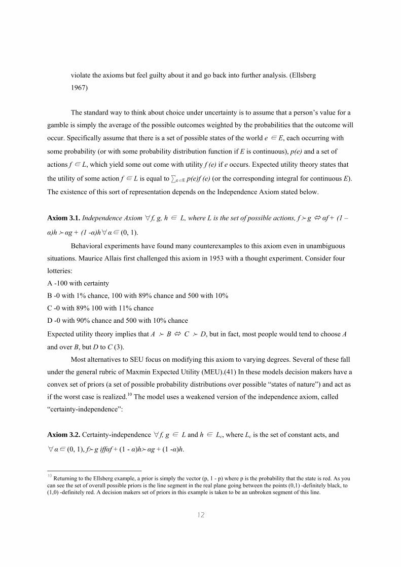
violate the axioms but feel guilty about it and go back into further analysis. (Ellsberg

1967)

The standard way to think about choice under uncertainty is to assume that a person’s value for a

gamble is simply the average of the possible outcomes weighted by the probabilities that the outcome will

occur. Specifically assume that there is a set of possible states of the world e ∈ E, each occurring with

some probability (or with some probability distribution function if E is continuous), p(e) and a set of

actions f ∈ L, which yield some out come with utility f (e) if e occurs. Expected utility theory states that

the utility of some action f ∈ L is equal to ∑e∈E p(e)f (e) (or the corresponding integral for continuous E).

The existence of this sort of representation depends on the Independence Axiom stated below.

Axiom 3.1. Independence Axiom ∀f, g, h ∈ L, where L is the set of possible actions, f f g αf + (1 –

α)h f αg + (1 -α)h∀α∈ (0, 1).

Behavioral experiments have found many counterexamples to this axiom even in unambiguous

situations. Maurice Allais first challenged this axiom in 1953 with a thought experiment. Consider four

lotteries:

A -100 with certainty

B -0 with 1% chance, 100 with 89% chance and 500 with 10%

C -0 with 89% 100 with 11% chance

D -0 with 90% chance and 500 with 10% chance

Expected utility theory implies that A f B C f D, but in fact, most people would tend to choose A

and over B, but D to C (3).

Most alternatives to SEU focus on modifying this axiom to varying degrees. Several of these fall

under the general rubric of Maxmin Expected Utility (MEU).(41) In these models decision makers have a

convex set of priors (a set of possible probability distributions over possible “states of nature”) and act as

if the worst case is realized.10 The model uses a weakened version of the independence axiom, called

“certainty-independence”:

Axiom 3.2. Certainty-independence ∀f, g ∈ L and h ∈ Lc, where Lc is the set of constant acts, and

∀α∈ (0, 1), ff g iffαf + (1 - α)hf αg + (1 -α)h.

10 Returning to the Ellsberg example, a prior is simply the vector (p, 1 - p) where p is the probability that the state is red. As you can see the set of overall possible priors is the line segment in the real plane going between the points (0,1) -definitely black, to (1,0) -definitely red. A decision makers set of priors in this example is taken to be an unbroken segment of this line.

13

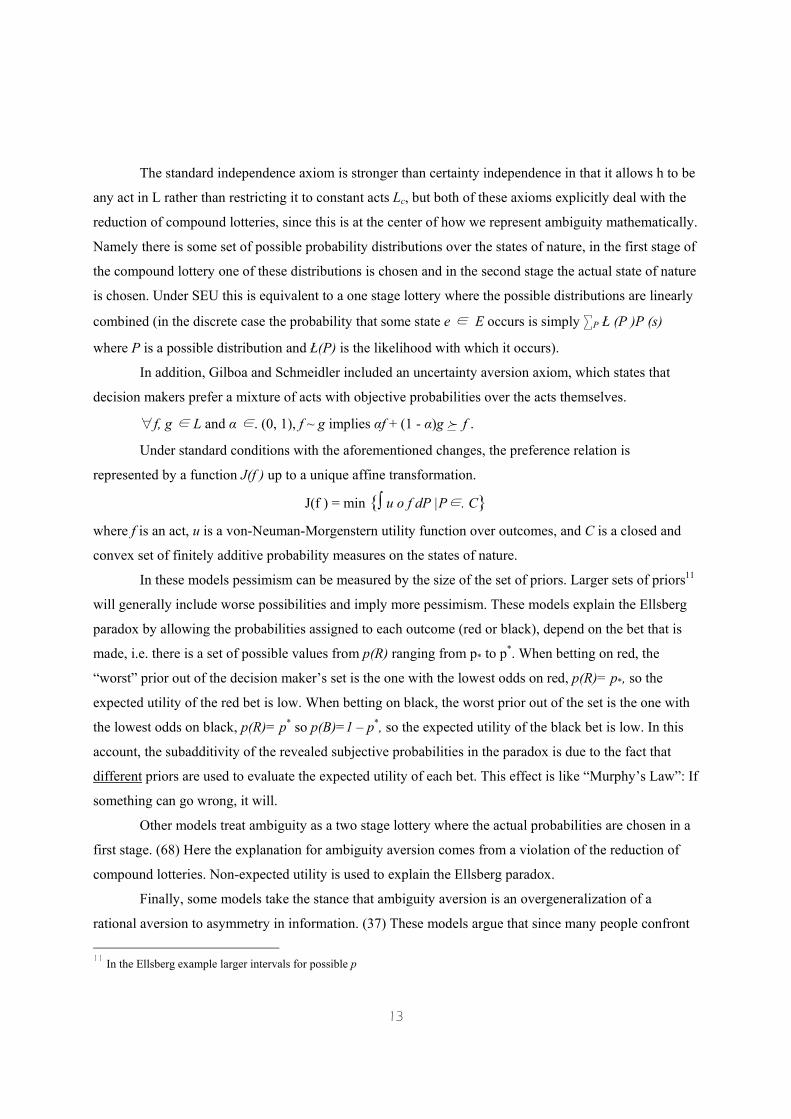
The standard independence axiom is stronger than certainty independence in that it allows h to be

any act in L rather than restricting it to constant acts Lc, but both of these axioms explicitly deal with the

reduction of compound lotteries, since this is at the center of how we represent ambiguity mathematically.

Namely there is some set of possible probability distributions over the states of nature, in the first stage of

the compound lottery one of these distributions is chosen and in the second stage the actual state of nature

is chosen. Under SEU this is equivalent to a one stage lottery where the possible distributions are linearly

combined (in the discrete case the probability that some state e ∈ E occurs is simply ∑P Ł (P )P (s)

where P is a possible distribution and Ł(P) is the likelihood with which it occurs).

In addition, Gilboa and Schmeidler included an uncertainty aversion axiom, which states that

decision makers prefer a mixture of acts with objective probabilities over the acts themselves.

∀f, g ∈ L and α ∈. (0, 1), f ~ g implies αf + (1 - α)g f f .

Under standard conditions with the aforementioned changes, the preference relation is

represented by a function J(f ) up to a unique affine transformation.

J(f ) = min {∫ u ο f dP |P∈. C}

where f is an act, u is a von-Neuman-Morgenstern utility function over outcomes, and C is a closed and

convex set of finitely additive probability measures on the states of nature.

In these models pessimism can be measured by the size of the set of priors. Larger sets of priors11

will generally include worse possibilities and imply more pessimism. These models explain the Ellsberg

paradox by allowing the probabilities assigned to each outcome (red or black), depend on the bet that is

made, i.e. there is a set of possible values from p(R) ranging from p* to p*. When betting on red, the

“worst” prior out of the decision maker’s set is the one with the lowest odds on red, p(R)= p*, so the

expected utility of the red bet is low. When betting on black, the worst prior out of the set is the one with

the lowest odds on black, p(R)= p* so p(B)=1 – p*, so the expected utility of the black bet is low. In this

account, the subadditivity of the revealed subjective probabilities in the paradox is due to the fact that

different priors are used to evaluate the expected utility of each bet. This effect is like “Murphy’s Law”: If

something can go wrong, it will.

Other models treat ambiguity as a two stage lottery where the actual probabilities are chosen in a

first stage. (68) Here the explanation for ambiguity aversion comes from a violation of the reduction of

compound lotteries. Non-expected utility is used to explain the Ellsberg paradox.

Finally, some models take the stance that ambiguity aversion is an overgeneralization of a

rational aversion to asymmetry in information. (37) These models argue that since many people confront

11 In the Ellsberg example larger intervals for possible p

14

incomplete information when they are facing a better informed opponent, they treat the Ellsberg paradox

as if there is asymmetric information (i.e., they act like they are playing a game against a malevolent

experimenter who is trying to trick them). We examine this “hostile opponent” hypothesis with the third

treatment in our study, where they actually play against a better-informed opponent.

At some point in the future, economic theories might specify not only the link between

unobservable factors and observed choices (such as beliefs and bet choices), but also a claim about neural

circuitry that implements observed choices. Reviewing the many theoretical papers on ambiguity, we

found only one suggestion about neural activity, in Raiffa (1963). He writes:

But if certain uncertainties in the problem were in cloudy or fuzzy form, then very often

there was a shifting of gears and no effort at all was made to think deliberately and

reflectively about the problem. Systematic decomposition of the problem was shunned

and an over-all ’seat of the pants’ judgment was made which graphically reflected the

temperament of the decision maker.

Raiffa’s suggestion seems to be that under ambiguity, deliberation and reflection (thought to be activities

in prefrontal cortex) are limited, and a temperamental “seat of the pants” judgment takes over.

Unfortunately, the seat of the pants is not a brain area but we could interpret him more broadly as

suggesting a rapid emotional reaction to ambiguity. Thus, we translate Raiffa’s observation, in neural

terms, as implying a more rapid emotional reaction to ambiguous choices than to risky ones.

3.2. Experimental Design. We explored the neural differences with varying levels of uncertainty by

using a combination of fMRI data and behavioral data from lesion patients. The fMRI study used three

experimental treatments: Bets on card decks (based on the Ellsberg example above); bets

15

FIGURE 1. Sample screens from the experiment. The top-panel conditions are called ambiguous because the subject is missing relevant information that is available in the risk conditions (bottom-panel). Subjects always choose between betting on one of the two options on the left side or taking the certain payoff on the right. (A) Card-deck treatment: Ambiguity is not knowing the exact proportion, risk is knowing the number of cards (indicated by numbers above each deck). (B) Knowledge treatment: Ambiguity is knowing less about the uncertain events (e.g., Tajikistan) relative to risk (e.g., New York City). (C) Hostile opponent treatment: Ambiguity is betting against an opponent who has more information (who drew a three-card sample from the deck) than risk (where the opponent drew no cards from the deck). Bets win if the subject chooses the realized color and opponent chooses the opposite color, if both players choose the same color they take the sure payoff.

on high-and low-knowledge world events; and bets against an informed or uninformed opponent (Fig. 1).

The card deck treatment is a baseline pitting pure risk, where probabilities are known with

certainty, against pure ambiguity. The knowledge treatment uses choices about events and facts, which

fall along a spectrum of uncertainty from risk to ambiguity. From the perspective of the MEU model, the

high-knowledge questions correspond to smaller sets of priors than the low-knowledge question.

The hostile opponent’s treatment offers bets against another person, who is either better-informed

or equally-informed about the contents of an ambiguous deck than the subject. In this condition the

“opponent” draws a sample of cards from an ambiguous deck before making his bet. The subject has the

option of making a simultaneous bet, but this will only count if the subject bets on the opposite color of

the color the informed opponent chose. Since the opponent should always bet on the majority color from

his sample, the subject’s bet will only count when it is on the minority color from a random sample in the

16

deck, i.e. when the subject is more likely to lose than win. This implies that the subject’s expected value

from winning is lower when the opponent is informed.12

Notice that all three treatments have one condition where the subjects are missing some relevant

information relative to the other. We call all these treatments the ambiguous conditions and the other

treatments the risky conditions. Subjects made 24 choices in each treatment between certain amounts of

money and bets on events. The amount of the certain payoff and the bet varied across trials.

In these experiments we allow at 6-8 seconds between trials. This break was necessary to allow

the activations caused by the previous trial to dissipate. We also randomize the length of these intertrial

intervals, because using a fixed interval can create anticipation effects in the seconds just before the new

trial is presented; these effects are diminished by having a random intertrial interval length.

For each treatment, we estimated a general linear model (GLM) using standard regression

techniques. Two primary regressors were used in the GLM, one for the ambiguity trials and one for the

risky trials. The regressors were constructed in the following way: first we created a boxcar regressor

(dummy variable) that was 1 during the risky (ambiguous) trial and 0 elsewhere. These regressors were

then convolved with a “hemodynamic response function”, this function allows us to take into account the

fact that the increase in oxygenated blood to an area of the brain is lagged and the time series has a

distinctive shape. Maximum likelihood estimation was used to fitt:

Bt = ßambAt +ßriskRt + ß0

where {Bt} is the time series for some voxel in the brain13. Voxels with regression coefficients

significantly different from 0 can be said to covary with either risk or ambiguity. We are mostly interested

in which voxels are differentially activated by ambiguity with respect to risk, i.e. voxels where ßamb is

significantly different from ßrisk.

As the experiment was self-paced, the length of the trials varied14. To find areas differentially activated

by ambiguity and risk across all three treatments, a one-way ANOVA of the three conditions was

12 For example, assume that the subject has a prior that the deck will either contain 5 red cards and 15 blue cards or 15 red cards and 5 blue cards. Assume that the opponent draws one card before choosing how to bet, and the opponent always bets on the color that he drew. The subject, having no information about the deck, will bet randomly on red or blue. Suppose the subject chooses to bet on red (without loss of generality). When the deck has 5 red cards and 15 blue cards, the opponent will draw a blue with probability ¾. As a result, the subject will end up betting against the opponent’s blue draw 75% of the time, and winning that bet only ¼ of the time. One-quarter of the time, the opponent draws a red card and bets red, in which case the subject’s red bet does not count (and the subject earns the sure amount c). Therefore, the subject’s expected value, conditional on the deck having 15 blue cards, is ¾ ¼x+ ¼c. The expected value conditional on the deck having 15 red cards is ¾c + ¼ ¾x. Since each of these conditional expected values is equally likely, the overall expected value is c/2 + 3/16 x. When the informed opponent does not have better information, then both subjects bet randomly and the subject’s expected value is c/2 + x/4 (since half the time their colors match and they earn c, and half the time they bet and the subject wins that bet half the time). Comparing the two expected values, there is a small drop in expected value (x/4 - 3/16x = x/16) when betting against the informed opponent. This drop leads to a stricter constraint on when it is rational to take the gamble (x> 8/3c instead of x> 2c). 13 The time series Bt for each voxel went through a high-pass filter and an AR(1) correction. 14 Mean response times were 6.39 secs (ambiguity) and 6.16 secs (risk), and were not significantly different.

17

performed, correcting for non-sphericity, and excluding areas that are significantly different between the

three treatments.

The regressors were anchored to stimulus presentation, i.e. the original dummy variable turns

“on” when the stimulus is presented as opposed to when a decision is made, based on the hypothesis that

the reaction to uncertainty would occur before the decision. We also analyzed the time courses of

activation anchored at both the stimulus onset and the decision time but did not find anything interesting

when compared to the stimulus-to-decision “epoch”.

3.3. Results.

3.3.1. fMRI Study. Areas that were more active during the ambiguous condition relative to the risk

condition are listed in Table 1. These included OFC and amygdala (Fig. 2a & b). Critchley et al found

OFC activation as subjects anticipated information about a financial gain or loss. (25) Our study shows

activity in this area even though there is no feedback during the experiment. More subtly the OFC appears

to be involved in integrating emotional and cognitive information. OFC lesion patients often behave

inappropriately in social situation despite knowledge of what proper behavior entails (10). So the OFC

may be active generally in emotional integration over a wide spectrum of situations.

The amygdala has been specifically implicated in processing information related to fear, e.g.

recognizing frightened faces. (7; 2; 24) We hypothesized that this area would be important for processing

uncertain events since risk and ambiguity aversion could be interpreted as fear of the unknown.15 In

addition the role of the amygdala in reacting to missing information is consistent with evidence of its

involvement in interpersonal evaluations with missing social information, where familiarity modulates

amygdala response. (61) Showing unfamiliar black faces to white subjects elicits amygdala activation

which correlates with the strength of implicit associations between black names and negatively-valenced

words (61). This correlation disappears when the black faces are familiar (e.g., Bill Cosby), which

suggests the amygdala may be partly reacting to ambiguity of the social evaluation of faces; activity

dissipates when faces are familiar and more like risky gambles which have less missing social

information. Similarity of activity in all three fMRI treatments also suggests that aversion to betting on

ambiguous events may be an overgeneralization of a rational aversion to betting against other agents who

are better-informed.

Areas activated during the risk condition relative to ambiguity are listed in Table 2. These include

the dorsal striatum (caudate nucleus) (Fig. 3a), an area that has been implicated in reward prediction. (67;

15 The amygdala is also involved in emotional learning and conditioning, both of which should be relevant in dealing with ambiguous situations (60).

18

58; 48) One earlier study (62) also found differential activation in the caudate during risk relative to

ambiguity using PET.16

Time courses also showed different patterns of activation in the ambiguity > risk and risk >

ambiguity regions indicating two distinct systems at work. Whereas the amygdala and OFC reacted

rapidly at the onset of the trial (Fig. 2c), the dorsal striatum activity built more slowly and peaks after the

decision time (Fig. 3b). Furthermore, these activations are present in all three experimental treatments17

(see Figures 4 and 5).

One simplified way of interpreting this data is to hypothesize that there are two interacting

systems (1) a vigilance system in the amygdala and OFC that responds more rapidly to the stimuli, and

(2) a reward-anticipation system in the striatum that is further downstream. The overall activity

differences in the contrasts indicate that system (2) is more active during risky decisions, which make

sense since in these situations subjects have the information necessary for accurate reward prediction.

Conversely, during ambiguous conditions, the first rapid system (1) appears to be more active, indicating

that it may be reacting to the level of information available (less information during the ambiguous

situations leads to greater vigilance in the form of higher activation levels in the amygdala and OFC).

Both systems are active to varying degrees during risky and ambiguous trials, the difference is one of

degree: as the level of information available to the decision maker rises, activity in system (1) declines

relative more ambiguous situations; the converse is true of system (2).

16 (see the RC-AC image at http://www.econ.umn.edu/ arust/neuroecon.html). 17 Note that it is rational in the hostile opponent’s treatment to discount some of the payoff in the gamble, as the gamble only wins if the better-informed opponent chose the wrong color. The hostile opponent hypothesis is that bets on ambiguous card decks and low-knowledge events, while normatively different than bets against the hostile opponent, are generated by similar neural circuitry. The time courses in the amygdala, OFC, and striatum are similar across all three treatments, consistent with this hypothesis.

19

FIGURE 2. Regions showing greater activation to ambiguity than risk: Random effects analysis of all three treatments revealed regions that are differentially activated in decision making under ambiguity relative to risk (at p . 0.001, uncorrected). These regions include (A) left amygdala, and right amygdala/parahippocampal gyrus, (B) bilateral OFC, and bilateral inferior parietal lobule (Table S2). (C) Mean time courses of amgydala and OFC (time synched to trial onset, dashed vertical lines are mean decision times; error bars are SEM; n=16). Time courses are plotted using the most signi.cant voxel in each cluster.

We measure the degree of ambiguity aversion for each subject and see if this correlates with brain

activity in a between-subjects analysis. The subjects’ utility functions for money are assumed to

20

FIGURE 3. Regions showing greater activation under risk than ambiguity: Random effects analysis of all three treatments revealed brain regions that are differentially activated in decision making under risk. These regions include (A) dorsal striatum, and also precuneus and premotor cortex (Table S3). (B) Mean time courses for risk areas (time synched to trial onset, dashed vertical lines are mean decision times; error bars are SEM; n=16). (C) These dorsal striatal areas were significantly correlated with the expected value of the subjects’ choices in the risk condition of the Card-Deck treatment (red, right), and both risk and ambiguity conditions of the Knowledge treatment (blue, left), p< 0.005. The laterality of these activations is consistent with the fact that language processing tends to occur in the left brain, while more abstract mathematical processing tends to occur in the right brain.

follow a power function u(x, ρ)= xρ, which is conveniently characterized by one parameter and widely

used in empirical estimation of this sort. Subjects are assumed to weight probabilities according to the

function π(p, γ)= pγ. The ρ parameter is interpreted as the risk aversion coefficient, i.e., the curvature of

the utility function. The p parameter is interpreted as the ambiguity aversion coefficient, i.e., how much

do people over(under)-weight probabilities because they are not confident in their judgments. If subjects

over-weight ambiguous probabilities (γ < 1), we characterize them as ambiguity-preferring. If they under-

weight ambiguous probabilities (γ > 1, as in the nonadditive prior view), we characterize them as

ambiguity-averse. If subjects weight probabilities linearly (p =1), we characterize them as ambiguity-

neutral. We assume subjects combine these weighted-probabilities and utilities linearly, so that their

weighted subjective expected utility is U (p, x, γ, ρ)= π (p, γ)u(x, ρ).

The tasks are all binary choices in which subjects either choose a gamble to win x (with

probability p) or 0, or a certain payoff c. For the risky deck, the ratios of the cards are the probabilities.

For the ambiguous decks and all knowledge questions, we assumed p =1/2. If subjective p is different

than 1/2 (e.g., because a subject happens to know a lot about fall temperatures in New York), then

21

subjective probabilities are not held constant across the knowledge trials. This possibility biases our

analysis against finding common regions of activation across treatments, so would

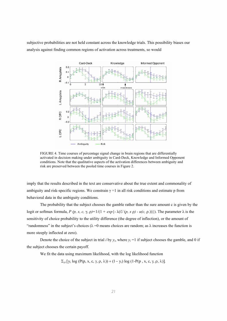
FIGURE 4. Time courses of percentage signal change in brain regions that are differentially activated in decision making under ambiguity in Card-Deck, Knowledge and Informed Opponent conditions. Note that the qualitative aspects of the activation differences between ambiguity and risk are preserved between the pooled time courses in Figure 2.

imply that the results described in the text are conservative about the true extent and commonality of

ambiguity and risk-specific regions. We constrain γ =1 in all risk conditions and estimate p from

behavioral data in the ambiguity conditions.

The probability that the subject chooses the gamble rather than the sure amount c is given by the

logit or softmax formula, P (p, x, c, γ, ρ)=1/(1 + exp{- λ(U (p, x ρ) - u(c, ρ.))}). The parameter λ is the

sensitivity of choice probability to the utility difference (the degree of inflection), or the amount of

“randomness” in the subject’s choices (λ =0 means choices are random; as λ increases the function is

more steeply inflected at zero).

Denote the choice of the subject in trial i by yi, where yi =1 if subject chooses the gamble, and 0 if

the subject chooses the certain payoff.

We fit the data using maximum likelihood, with the log likelihood function

Σyi [yi log (P(p, x, c, γ, ρ, λ)) + (1− yi) log (1-P(p , x, c, γ, ρ, λ)].

22

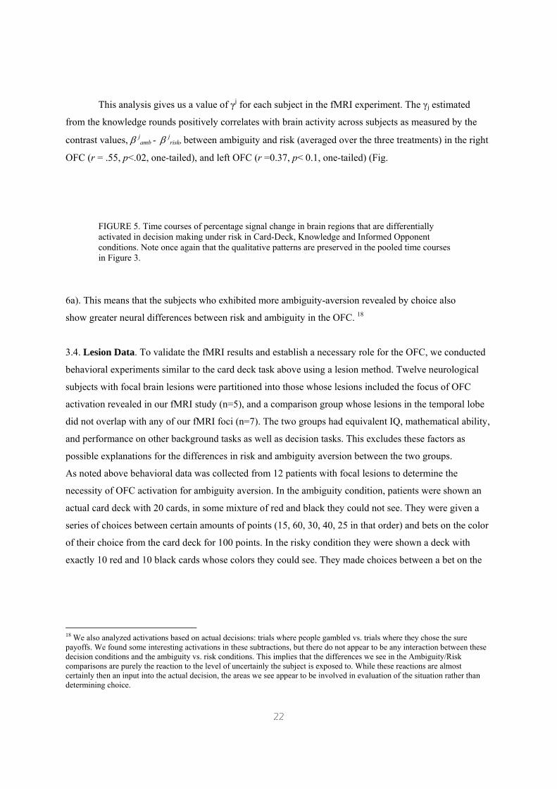
This analysis gives us a value of γj for each subject in the fMRI experiment. The γj estimated

from the knowledge rounds positively correlates with brain activity across subjects as measured by the

contrast values, β jamb - β jrisk, between ambiguity and risk (averaged over the three treatments) in the right

OFC (r = .55, p<.02, one-tailed), and left OFC (r =0.37, p< 0.1, one-tailed) (Fig.

FIGURE 5. Time courses of percentage signal change in brain regions that are differentially activated in decision making under risk in Card-Deck, Knowledge and Informed Opponent conditions. Note once again that the qualitative patterns are preserved in the pooled time courses in Figure 3.

6a). This means that the subjects who exhibited more ambiguity-aversion revealed by choice also

show greater neural differences between risk and ambiguity in the OFC. 18

3.4. Lesion Data. To validate the fMRI results and establish a necessary role for the OFC, we conducted

behavioral experiments similar to the card deck task above using a lesion method. Twelve neurological

subjects with focal brain lesions were partitioned into those whose lesions included the focus of OFC

activation revealed in our fMRI study (n=5), and a comparison group whose lesions in the temporal lobe

did not overlap with any of our fMRI foci (n=7). The two groups had equivalent IQ, mathematical ability,

and performance on other background tasks as well as decision tasks. This excludes these factors as

possible explanations for the differences in risk and ambiguity aversion between the two groups.

As noted above behavioral data was collected from 12 patients with focal lesions to determine the

necessity of OFC activation for ambiguity aversion. In the ambiguity condition, patients were shown an

actual card deck with 20 cards, in some mixture of red and black they could not see. They were given a

series of choices between certain amounts of points (15, 60, 30, 40, 25 in that order) and bets on the color

of their choice from the card deck for 100 points. In the risky condition they were shown a deck with

exactly 10 red and 10 black cards whose colors they could see. They made choices between a bet on the

18 We also analyzed activations based on actual decisions: trials where people gambled vs. trials where they chose the sure payoffs. We found some interesting activations in these subtractions, but there do not appear to be any interaction between these decision conditions and the ambiguity vs. risk conditions. This implies that the differences we see in the Ambiguity/Risk comparisons are purely the reaction to the level of uncertainly the subject is exposed to. While these reactions are almost certainly then an input into the actual decision, the areas we see appear to be involved in evaluation of the situation rather than determining choice.

23

color of their choice from the deck for 100 points, or certain amounts of 30, 60, 15, 40, and 25 (in that

order, see Table 1)19 .

We could estimate ρ and γ for each individual in the fMRI study. We were, however, forced to pool data

within each patient group because there are not enough data points to estimate each patient’s parameter.

The behavioral data were pooled and a bootstrap procedure was used to create 100 pseudosamples with

corresponding (γ, ρ) pairs. Two-dimensional confidence interval analysis of these pairs (Fig. 6b) shows

that frontal patients are risk-and ambiguity-neutral (i.e., the hypothesis that γ =ρ =1 cannot be rejected).

This behavior of frontal patients was significantly different than the damage control group, who were

averse to both risk and ambiguity. The OFClesioned group was therefore abnormally neutral toward

ambiguity (which is, ironically, a hallmark of rationality under SEU).

The parameter γ enables us to link the fMRI and lesion studies. Assume that the frontal patients

would have a right OFC (ROFC) contrast value of zero if they were imaged during these tasks (since all

have ROFC damage). Then we can guess what value of γ the OFC patients might exhibit behaviorally, by

extrapolating correlation between ROFC activity and γ in Figure 6a to the case where there is zero

activity in ROFC. This extrapolation gives a predicted γ = .85. The actual value estimated from the OFC

patients’ behavioral choices is γ = .82, which is reasonably close to the extrapolated prediction.

3.5. Discussion. The two hypothesized systems, amygdala/OFC, and striatum are active in both

ambiguity and risk; the differences in activation between the two are driven by the level of uncertainty in

the different conditions. The fact that we see similar activation patterns for the real-world treatment as the

card-deck treatment supports the hypothesis that risk and ambiguity are in fact points on a spectrum of

uncertainty rather than two completely different entities. The reaction of the amygdala and OFC seems to

be tied to the level of perceived uncertainty. That these areas are also activated by the hostile-opponent

treatment indicates that the reaction to uncertainty is an instance of a more general “vigilance” reaction to

possibly dangerous situations.

An interesting implication of this study is that models of risk and ambiguity that treat the two as

quantitatively instead of qualitatively different may be more neurally and therefore behaviorally accurate.

The current models of risk aversion relying solely on the curvature of the utility function do not allow for

this. The implication that both types of aversion are the result of a direct dampening of activity in the

dorsal striatum, which may well be the internal representation of utility in the brain, could help resolve

19 There are three small differences in this task and the Card-Deck treatment in the fMRI experiment: (1) There were fewer choices in the lesion experiment, due to time constraints in conducting experiments with lesion patients and the need for multiple trials to extract fMRI signal; (2) there was wider range of certain point amounts in the lesion task (in case patients were extremely risk-and ambiguity-averse or -preferring); and (3) due to human subjects restrictions, the lesion task choices were not conducted for actual monetary payments.

24

some of the paradoxes of risk aversion as well as ambiguity aversion, for example the vastly different

expressions of risk over small verses large bets.

The regions implicated in our fMRI experiments and confirmed by behavioral experiments with

lesion patients have been observed in previous studies using different tasks. The striatum-amygdala-OFC

network is well-established in animal and human studies as a system for reward learning, including

probabilistic learning (25). The OFC is highly interconnected with the basolateral amygdala. These

interconnections appear to play vital roles in learning and reversal learning in rats (66).

FIGURE 6. A) Regression of right OFC contrast values on the behavioral measure of ambiguity γ (calibrated from knowledge questions). B) Measures of risk (ρ) and ambiguity (γ) preferences of OFC (n =5) and control group (n =7). The risk neutral line (γ = 1) and the ambiguity neutral line (p = 1) demarcate four quadrants as labeled. Open symbols plot ML estimates of a group-level stochastic choice model (frontals: (γ =0.82, ρ =1.09); lesion controls: (γ =1.23, ρ = 0.74)). Solid symbols represents 100 bootstrapped (γ,ρ) estimates. Ellipses are two-dimensional 90% confidence intervals around the bootstrapped data. Angle of the ellipse reflects correlation between ρ and γ (0.42 for frontal, 0.31 for control). Lateral OFC, in particular, appears to be necessary to change existing associations (57). Our

finding that the OFC is activated as a function of ambiguity, and that its damage reduces sensitivity to

ambiguity, suggest that this structure is a necessary component for reacting to gradations of uncertainty.

25

The idea that ambiguity aversion in card deck and knowledge choices is related to rational aversion to

betting against a better informed opponent (the hostile opponent hypothesis) is supported by similarities

in time courses in the amygdala, OFC, and striatum between all three treatments.

We present evidence that the human brain responds to varying levels of uncertainty, contrary to

many decision theories which regard choices under risk and ambiguity as equivalent. FMRI data suggests

that uncertainty is represented in a system that includes the amygdala and OFC.

Both the amygdala and OFC are known to receive rapid, multi-modal sensory input; both are

bidirectionally connected and known to function together in evaluating the value of stimuli (38); and both

are likely involved in the detection and salient, relevant, and ambiguous stimuli. The latter function has

been hypothesized especially for the amygdala (72; 1). Critically, such a function also provides a reward-

related signal that can motivate behavior, in virtue of the known connections between the amygdala/OFC

and the striatum (5). Under ambiguity, the brain is alerted to the fact that information is missing, that

choices based on the information available therefore carry more unknown (and potentially dangerous)

consequences, and that cognitive and behavioral resources must be mobilized in order to seek out

additional information from the environment.

Understanding the neural basis of choice under uncertainty, in the broader sense including both

risk and ambiguity, is important because it is a fundamental activity at every societal level, from

retirement savings, to insurance pricing, to determining international military policy. These choices vary

not only because of the presence of uncertainty, but the perceived level of uncertainty. Our results suggest

that we pursue a unified model of uncertainty which would treat risk and ambiguity as points on a larger

continuous scale. The knowledge treatment of the experiment further implies that the relevant level of

uncertainty might be a function of mathematically unrelated factors, such as familiarity with related but

irrelevant information.

Finally, economists should care about understanding the neural basis of decision only if the extra

level of detail helps us make predictions that standard economic theories would not make. For example,

the evidence above suggests that the amygdala and OFC participate in evaluating the degree of

uncertainty, generating an aversion to ambiguity, and also signaling a larger anticipated reward from risky

bets to the striatum. Knowing that these particular areas are part of a candidate circuit is most useful for

economics if we know something special about their properties and other functions they perform.

Fortunately, a lot is known about the amygdala’s structure and function. It is rapidly activated by

exposure to fearful stimuli (as briefly as 5-15 milliseconds of exposure to a fearful face (72)).

Furthermore, it is possible that if there are competing stimuli which influence the amygdala, then the OFC

cannot disentangle which stimulus generates the influence. These two properties lead to the following

26

prediction: Suppose the amygdala is stimulated by some fear-inducing stimulus which is independent of

an ambiguous bet, such as anticipation of an impending electric shock a few seconds later. While waiting

for the potential shock, the subject chooses between a sure amount or an ambiguous bet. If the OFC

mistakes the amygdala activity from the shock anticipation for a fear of betting under ambiguity, then the

subject may be more averse to ambiguous bets when a shock is anticipated (compared to control

conditions when there is no shock anticipation). We do not know if this experiment will work; if the OFC

can separate the influence of shock-anticipation fear from ambiguity-aversion-driven fear then the

experiment will not work. But if the experiment does show an effect, then we have a very powerful

challenge to the standard idea in economics of stable preferences. Adding the shock anticipation will have

essentially changed the expressed preference, not because we have truly changed the degree of aversion to

ambiguous bets, but because we used our knowledge of the components of circuitry to trick the OFC into

thinking the amygdala was afraid of the bet rather than afraid of the shock.

This phenomenon could even be incorporated into a theoretical model using standard parts from

the economic theory hardware store. Suppose the amygdala is activated by various state variables (shock

anticipation, fearful faces, ambiguous bets, etc.). The amygdala observes a state variable and sends a

signal to the OFC. (This is like an infant who is crying, but the crying itself does not signal to a concerned

parent what condition – hunger, pain, fatigue – caused the crying.) The OFC gets the signal but does not

observe the state variable. The OFC must then make a decision, such as pricing an ambiguous gamble.

Since the OFC does not know the source of fear, it implements more aversion to ambiguity.

4. CONCLUSION

The goal of neuroeconomics is to ground economic theory in details of how the brain works in

decision making, strategic thinking, and exchange. One way to achieve this is to observe processes and

constructs which are typically considered unobservable, to decide between many theories of behavioral

anomalies like risk aversion, altruistic punishment, and reciprocity. Another likely outcome is that

thinking about brain details will provide a new way of understanding concepts which have been

traditionally left out of economic analysis, like emotion, willpower, habit, and the biological basis of

demand. No one neuroeconomic study will be able to conclusively do either of these things, but by

combining experiments and types of data we may gain insights into behavior that we cannot arrive at by

introspection of behavioral observation.

The study discussed in this paper illustrates both of these goals to varying degrees. First, it allows

us to use neural evidence to discount models of ambiguity that treat is as merely a two stage lottery by

showing that there may be two interacting systems determining the experienced utility of an option, one

responding to the level of information in general and one that uses input from this system to discount the

27

reward of the possible results. Second it suggests a substantially different way to look at risk-aversion.

Considering a more general uncertainty aversion that dampens the utility of a gamble gets allows us to

consider careful models of risk where the context of the gamble is important, something that is very

difficult if we only consider a single universal utility function.

28

29

30

REFERENCES

1. ADAMS, R., GORDON, H., BAIRD, A., AMBADY, N., AND KLECK, R. Effects of gaze on

amygdala sensitivity to anger and fear faces. Science 300, 5625 (Jun 2003), 1536.

2. ADOLPHS, R. Neural systems for recognizing emotion. Curr. Opin. Neurobiol. 12 (2002), 169–177.

3. ALLAIS, M. Le comportement de l’homme rationnel devant le risque: Critique des postulats et

axiomes de l’´ecole am´ericaine. Econometrica 21 (1953), 503–546.

4. AMADI, A. Equity home bias: A disappearing phenomenon. http://ssrn.com/abstract=540662, 2004.

5. AMARAL, D., PRICE, J., PITKANEN, A., AND CARMICHAEL, S. Anatomical organization of the

primate amygdaloid complex. In The Amygdala: Neurobiological Aspects of Emotion, Memory, and

Mental Dysfunction, J. P. Aggleton, Ed. Wiley, New York, 1992.

6. BAYLEY, P. J., FRASCINO, J. C., AND SQUIRE, L. R. Robust habit learning in the absence of

awareness and independent of the medial temporal lobe. Nature 436 (2005), 550–553.

7. BECHARA, A., DAMASIO, H., AND DAMASIO, A. Role of the amygdala in decision-making.

Ann. N.Y. Acad. Sci. 985 (2003), 356–369.

8. BECKER, S., AND BROWNSON, F. What price ambiguity? on the role of ambiguity in decision

making. J. Pol. Econ. 72 (1964), 62–73.

9. BERG, J., DICKHAUT, J., AND MCCABE, K. Trust, reciprocity and social history. Games and

Economic Behavior 10, 1 (1995), 122–142.

10. BERTHOZ, S., ARMONY, J., BLAIR, R., AND DOLAN, R. An fmri study of intentional and

unintentional (embarrassing) violations of social norms. Brain 125 (2002), 1696–1708.

11. BEWLEY, T. Knightian decision theory, part i. Decisions in Economics and Finance 25 (2002), 79–

110.

12. BHATT, M., AND CAMERER, C. F. Self-referential thinking and equilibrium as states of mind in

games: fmri evidence. Games and Economic Behavior 52, 2 (2005), 424–459.

13. BRUNI, L., AND SUGDEN, R. The road not taken: two debates about the role of psychology in

economics. In press.

14. BUSINO, G. Note bibliographique sur le cours. In Vilfredo Pareto. Epstolario. Accademia Nazionale

dei Lincei, Rome, 1964, pp. 1165–1172.

15. CALDER, A. J., KEANE, J., MANES, F., ANTOUN, N., AND YOUNG, A. W. Impaired

recognition and experience of disgust following brain injury. Nature Neuroscience 3 (2000), 1077–

1078.

16. CAMERER, C., AND KARJALAINEN, R. Ambiguity-aversion and non-additive beliefs in non-

cooperative games: Experimental evidence. In Models and Experiments on Risk and Rationality, B.

Munier and M. Machina, Eds. Kluwer Academic Publishers, Dordrecht, 1994, pp. 325–358.

31

17. CAMERER, C., LOEWENSTEIN, G., AND PRELEC, D. Neuroeconomics: How neuroscience can

inform economics. J. Econ. Lit. 43 (2005), 9–63.

18. CAMERER, C., AND WEBER, M. Recent developments in modeling preferences: Uncertainty and

ambiguity. J. Risk Uncert. 5 (1992), 325–370.

19. CAMERER, C. F. Behavioral Game Theory: Experiments in Strategic Interaction. Princeton

University Press, Princeton, 2003.

20. CAMERER, C. F. Behavioral economics. Prepared for the World Congress of the Econometric

Society, 2005.

21. CAMERER, C. F., HO, T.-H., AND CHONG, J. K. A cognitive hierarchy theory of one-shot games.

Quarterly Journal of Economics 119 (2004), 861–898.

22. CHORVAT, T., AND MCCABE, K. Neuroeconomics and rationallity. George Mason University

School of Law: Law and Economics Working Paper Series.

23. COLANDER, D. Neuroeconomics, the hedonimeter, and utility: Some historical links. Middlebury

College, 2005.

24. CRITCHLEY, H., ELLIOT, R., MATHIAS, C., AND DOLAN, R. Neural activity relating to

generation and representation of galvanic sckin conductance responses: A functional magnetic

resonance imaging study. J. Neurosci. 20 (2000), 3033–3040.

25. CRITCHLEY, H., MATHIAS, C., AND DOLAN, R. Neural activity in the human brain relating to

uncertainty and arousal during anticipation. Neuron 29 (2001), 537–545.

26. DE QUERVAIN, D. J.-F., FISCHBACHER, U., TREYER, V., SCHELLHAMMER, M.,

SCHNYDER, U., BUCK, A., AND FEHR, E. The neural basis of altruistic punishment. Science 305

(2004), 1254–1258.

27. DOW, J., AND DACOSTA WERLANG, S. R. Uncertainty aversion, ris aversion and optimal choice

of portfolio. Econometrica 60 (1992), 197–204.

28. DUFF, P. The scottish criminal jury: A very peculiar institution. Law and Contemporary Problems 62

(1999), 173.

29. DUFWENBERG, M., AND GNEEZY, U. Measuring beliefs in an experimental lost wallet game.

Games and Economic Behavior 30 (2000), 163–182.

30. EFMA BASEL MEETINGS PAPER. Patriotism in Your Portfolio (2004).

31. EISENBERGER, N. I., LIEBERMAN, M. D., AND WILLIAMS, K. D. Does rejection hurt? and

fmri study of social exclusion. Science 302 (2003), 290–292.

32. ELLSBERG, D. Risk, ambiguity, and the savage axioms. The Quart. J of Econ. 75, 4 (1961), 643–

669.

32

33. EPSTEIN, L., AND WANG, T. Intertemporal asset-pricing under knightian uncertainty.

Econometrica 62 (1994), 283–322.

34. FOX, C., AND TVERSKY, A. Ambiguity aversion and comparative ignorance. Q. J. Econ. 110

(1995), 585–603.

35. FRENCH, K., AND POTERBA, J. Investor diversi.cation and international equity markets. American

Economic Review 81 (1991), 222–226.

36. FRIEDMAN, M. Essays in Positive Economics. University of Chicago Press, Chicago, 1953.

37. FRISCH, D., AND BARON, J. Ambiguity and rationality. J. Behav. Decision Making 1 (1988), 149–

157.

38. GAFFAN, D., MURRAY, E. A., AND FABRE-THORPE, M. Interaction of the amygdala with the

frontal lobe in reward memory. Eur. J. Neurosci. 5, 7 (Jul 1993), 968–975.

39. GALLAGHER, H. L., JACK, A. I., ROEPSTORFF, A., AND FRITH, C. D. Imaging the intentional

stance in a competitive game. NeuroImage 16 (2002), 814–821.

40. GHIRARDATO, P., AND KATZ, J. Indecistion theory: Explaining selective abstention in multiple

elections. J. Pub. Ec. Theory Forthcoming (2005).

41. GILBOA, I., AND SCHMEIDLER, D. Maxmin expected utility with non-unique prior. J. Math.

Econ. 18 (1989), 141–153.

42. GLIMCHER, P., AND RUSTICHINI, A. Neuroeconomics: The concilience of brain and decision.

Science 306 (2004), 447–452.

43. GRAHAM, J. R., HARVEY, C. R., AND HUANG, H. Investor competence, trading frequency, and

home bias. Available at http://ideas.repec.org/p/nbr/nberwo/11426.html, 2005.

44. GUL, F., AND PESENDORFER, W. The case for mindless economics.

http://www.dklevine.com/archive/refs4784828000000000581.pdf, 2005.

45. JEVONS, W. S. The Theory of Political Economy. Penguin, London, 1871/1970.

46. KAHNEMAN, D., AND TVERSKY, A. Prospect theory: An analysis of decision under risk.

Econometrica 42 (1979), 263–292.

47. KIM, H., AND WHALEN, P. J. A Computational Model of Amygdala-Basal Forebrain-Prefrontal

Cortex Interaction in the Detection and Resolution of Predictive Uncertainty. PhD thesis, University

of Wisconsin -Madison, 2004.

48. KNUTSON, B., ADAMS, C., FONG, G., AND HOMMER, D. Anticipation of monetary reward

selectively recruits nucleus accumbens. J. Neurosci. 21 (2001).

49. KOSFELD, M., HEINRICHS, M., ZAK, P., FISCHBACHER, U., AND FEHR, E. Oxytocin

increases trust in humans. Nature 435 (2005), 673–676.

33

50. LAIBSON, D. Golded eggs and hyperbolic discounting. The Quarterly Journal of Economics 112, 2

(1997), 443–477.

51. LO, K. C. Extensive form games with uncertainty averse players. Games Econ. Behav. 28 (1999),

256–270.

52. MACCRIMMON, K. Desciptive and normative implications of the decision-theory postulates. In

Risk and Uncertainty, K. Borch and J. Mossin, Eds. MacMillan, London, 1968.

53. MCCABE, K., HOUSER, D., RYAN, L., SMITH, V., AND TROUARD, T. A functional imaging

study of cooperation in two-person reciprocal exchange. Proceeding of the NAtional Academy of

Sciences 98 (2001), 11832–11835.

54. MCCLURE, S. M., LAIBSON, D., LOEWENSTEIN, G., AND COHEN, J. D. Separate neural

systems value immediate and delayed monetary rewards. Science 306 (2004), 503–507.

55. MUKERJI, S. Ambiguity aversionand incompleteness of information. Amer. Econ. Rev. 88 (1998),

1207–1231.

56. MUKERJI, S., AND TALLON, J.-M. An overview of economic applications of david schmeidler’s

models of decision making under uncertainty. In Uncertainty in Economic Theory: A collection of

essays in honor of David Schmeidler’s 65th Birthday, I. Gilboa, Ed. Routledge, 2004.

57. O’DOHERTY, J., CRITCHLEY, H., DEICHMANN, R., AND DOLAN, R. Dissociating valence of

outcome from response switching in human orbital and ventral prefrontal cortices. Neurosci. 23

(2003), 7931–7939.

58. O’DOHERTY, J., DAYAN, P., SCHULTS, J., DEICHMANN, R., FRISTON, K., AND DOLAN, R.

Dissociable roles of ventral and dorsal striatum in instrumental conditioning. Science 304 (2004),

452–454.

59. O’DONOGHUE, T., AND RABIN, M. Doing it now or later. American Economic Review 89, 1

(1999), 103–124.

60. PHELPS, E., DELGADO, M., NEARING, K., AND LEDOUX, J. Extinction learning in humans:

Role of the amygdala and vmpfc. Neuron 43 (2004), 897–905.

61. PHELPS, E., O’CONNOR, K., CUNNINGHAM, W., FUNAYAMA, E., GATENBY, J., GORE, J.,

AND BANAJI, M. Performance on indirect measures of race evaluation predicts amygdala activation.

J. Cog. Neuro. 12 (2000), 729–738.

62. RUSTICHINI, A., DICKHAUT, J., GHIRADATO, P., SMITH, K., AND PARDO, J. A brain

imaging study of the choice procedure. Games Econ. Behav. (in press).

63. SANFEY, A. G., RILLING, J. K., ARONSON, J. A., NYSTROM, L. E., AND COHEN, J. D. The

neural basis of economic decision-making in the ultimatum game. Science 300 (2003), 1755–1758.

34

64. SARGENT, T., AND HANSEN, L. Robust control and economic moded uncertainty. Unpublished

Monograph, available at http://homepages.nyu.edu/ ts43/BOOKS/booksframe.htm.

65. SCHMEIDLER, D. Subjective probablity and expected utility without additivity. Econometrica 57

(1989), 571–587.

66. SCHOENBAUM, G., CHIBA, A., AND GALLAGHER, M. Changes in functional connectivity in

orbitofrontal cortex and basolateral amygdala during learning and reversal training. Neuro. 20 (2000),

5179–5189.

67. SCHULTZ, W. Multiple reward signals in the brain. Nat. Rev. Neurosci. 1 (2000), 199–207.

68. SEGAL, U. The ellsberg paradox and risk aversion: An anticipated utility approach. International

Economic Review 28, 1 (1987), 175–202.

69. SIEGEL, J. Stocks for the Long Run, 2 ed. Irwin, New York, 1998.

70. STRONG, N., AND XU, X. Understanding the equity of home bias: evidence from survey data.

Revie of Economics and Statistics 85 (2003), 307–312.

71. WEIGELT, K., AND CAMERER, C. F. Reputation and corporate strategy: a review of recent theory

and implications. Strategic Management Journal 9 (1988), 443–454.

72. WHALEN, P. J. Fear, vigilance and ambiguity: initial neuroimaging studies of the human amygdala.

Curr. Dir. Psychol. Sci. 7, 6 (1998), 177–188.

73. ZAK, P. Neuroeconomics. Philosophical Trasactions of the Royal Society (In press).