
NEURO-FUZZY BASED HYBRID METHOD FOR ... Abstrak Peneutralan pH dianggap sebagai salah satu daripada...
119
NEURO-FUZZY BASED HYBRID METHOD FOR MODELING AND CONTROL OF PH NEUTRALIZATION MOHD FAUZI BIN ZANIL FACULTY OF ENGINEERING UNIVERSITY OF MALAYA KUALA LUMPUR 2012
Transcript of NEURO-FUZZY BASED HYBRID METHOD FOR ... Abstrak Peneutralan pH dianggap sebagai salah satu daripada...

NEURO-FUZZY BASED HYBRID METHOD FOR MODELING AND
CONTROL OF PH NEUTRALIZATION
MOHD FAUZI BIN ZANIL
FACULTY OF ENGINEERING
UNIVERSITY OF MALAYA
KUALA LUMPUR
2012

NEURO-FUZZY BASED HYBRID METHOD FOR MODELING AND
CONTROL OF PH NEUTRALIZATION
MOHD FAUZI BIN ZANIL
DISSERTATION SUBMITTED IN FULFILMENT OF THE
REQUIREMENTS FOR THE DEGREE OF
MASTER OF ENGINEERING SCIENCE
FACULTY OF ENGINEERING
UNIVERSITY OF MALAYA
KUALA LUMPUR

ii
Abstract
The pH neutralization is regarded as one of the fundamental parts of industrial chemical
process. In electrochemical industry for example, heavy metals must be recovered (by
reducing the solubility of the metals) from waste streams by controlling the pH value to
prevent polluting the environment.
The pH neutralization shows strong nonlinear characteristics because of feed condition.
Theoretically, the nonlinear effects for this process come from negative logarithm of
ionic hydrogen, where process dynamic occurs when the hydrogen ions increase or
decrease during neutralization process and because of dynamic nonlinearity called the
‘‘S-shape’’ curve which consists of extreme sensitivity and insensitivity regions.
This study proposes a hybrid model and a Fuzzy Logic controller for an on-line pH
neutralization pilot plant. The model is used to identify the on-line pH neutralization
plant’s characteristics and to improve the Fuzzy Logic controller decision output. The
hybrid model is between neuro-fuzzy (ANFIS) identification technique and first
principle model. The identification technique uses training dataset from experimental
data to map the neutralization response curve from pH equal to 3 to 11. The first
principle model is based on material balances and chemical equilibrium equation.
The objective of the proposed model is to extend the robustness effect in the Fuzzy
Logic controller by predicting the control action based on on-line titrations
characteristics without having to re-design the model if plant undergoes different
conditions. The on-line model validation and controller performance analysis for hybrid

iii
model and Fuzzy Logic controller was conducted and compared. The lowest values of
RMSE (Root Mean Square of Error) and ISE (Integral Square of Error) are desired to
justify the goodness of proposed model and controller respectively.
In the experiment, the hybrid model (in nominal plant condition, RSME = 0.1013 and in
altered plant condition, RMSE = 0.5616) gives best of fit for the on-line neutralization
process. The proposed Fuzzy Logic controller with inverse hybrid model is able to
handle the nonlinearity and robustness issues for the on-line pH neutralization. In set
point tracking analysis, it shows best performance (ISE = 35.032) compared to normal
Fuzzy Logic controller (ISE = 157.652) and PID controller (ISE =195.365). Thus, the
proposed hybrid model and the proposed Fuzzy Logic controller can be used effectively
in on-line/off-line studies of the dynamic behaviour of the pH neutralization pilot plant.

iv
Abstrak
Peneutralan pH dianggap sebagai salah satu daripada bahagian-bahagian asas proses
kimia di industri. Dalam industri elektrokimia sebagai contoh, logam berat mesti
dipisahkan (dengan mengurangkan keterlarutan logam) dari aliran sisa dengan
mengawal nilai pH bagi mencegah pencemaran alam sekitar. Peneutralan pH
menunjukkan ciri-ciri tak linear yang kuat adalah kerana kadar keadaan aliran masukan.
Secara teori, kesan tak linear bagi proses ini datang daripada logaritma negatif ion
Hidrogen, di mana dinamik proses berlaku apabila ion Hidrogen peningkatan atau
penurunan semasa proses peneutralan. Proses ketaklelurusan dinamik ini dipanggil
"bentuk-S" terdiri daripada rantau sensitiviti melampau dan kekurang sensitiv.
Kajian ini mencadangkan satu model hibrid dan pengawal Fuzzy Logic untuk
peneutralan pH secara on-line pada loji perintis. Hybrid model ini digunakan untuk
mengenal pasti ciri-ciri peneutralan pH secara on-linedan model ini dapat meningkatkan
keputusan keluaran pengawal Fuzzy Logic. Model hibrid adalah kombinasi antara
neuro-fuzzy (ANFIS) dan model prinsip pertama.Teknik pengenalan yang
menggunakan dataset latihan daripada data eksperimen adalah bagi tujuan pememetaan
keluk tindak-balas peneutralan pH daripada ph 3 hingga pH 11. Model prinsip yang
pertama adalah berdasarkan persamaan keseimbangan bahan dan persamaan
keseimbangan kimia.
Objektif model yang dicadangkan bertujuan untuk melanjutkan kesan kekukuhan dalam
pengawal Fuzzy Logic. Hal ini dapat dijayakan dengan meramalkan tindakan kawalan
yang bersesuaian berdasarkan ciri-ciri titratan dalam talian tanpa perlu mereka-bentuk
semula model atau pengawal jika loji perintis berubah keadaan yang berbeza.

v
Pengesahan model dalam talian dan analisis prestasi pengawal bagi model hibrid dan
pengawal Fuzzy Logic telah dijalankan dan dibandingkan. Nilai terendah bagi RMSE
(Root Mean Square Error) dan ISE (Integral of Square Error) adalah dikehendaki untuk
menunjukkan kebaikan model yang dicadangkan dan pengawal masing-masing.
Dalam eksperimen, model hibrid (pada keadaan logi nominal, RSME = 0.1013 dan
dalam keadaan logi yang diubah, RMSE = 0.5616) memberikan yang
terbaik yang layak untuk proses peneutralan on-line. Pengawal fuzzy logic dengan
model hibrid songsang yang dicadangkan adalah mampu menangani isu-isu
ketaklelurusan dan kekukuhan bagi peneutralan pH on-line. Dalam analisis pengesanan
titik set, ia menunjukkan prestasi yang terbaik (ISE = 35.032) berbanding pengawal
fuzzy logic yang biasa (ISE = 157.652) dan pengawal PID (ISE = 195.365). Oleh itu,
model hibriddan pengawal fuzzy logic yang dicadangkan boleh digunakan secara
berkesan dalam kajian kelakuan dinamik bagi logi perintis peneutralan pH secara on-
line /off-line.

vi
Acknowledgment
In the Name of Allah, the Beneficial and the Merciful.
First, I am grateful to my supervisor, Professor Ir. Dr. Mohd Azlan Hussain and co-
supervisor, Associate Professor Dr. Rosli Omar for their support and interest during my
postgraduate research.
Indeed, I could not have been able to complete my dissertation work without their
inspiration. I would like to thank the Chemical Engineering Department, University of
Malaya. I am indebted to Dr. Khairi Abdul Wahab and postgraduate classmate, Mr.
Shazzad Hossain at Chemical Engineering Department.
For financial support provided during my postgraduate study, I am grateful to E-Science
Fund and University Malaya Power Energy Dedicated Advanced Centre (UMPEDAC)
for financial support during the candidacy.
Finally, I would like to thank my parents, wife, brother, sisters, and families for their
support.

vii
Table of Contents
Abstract ............................................................................................................................ ii
Acknowledgment ............................................................................................................ vi
Table of Contents .......................................................................................................... vii
List of Figures ................................................................................................................. xi
List of Tables ................................................................................................................ xiii
Nomenclature................................................................................................................ xiv
Chapter 1 : Introduction .............................................................................................. 16
1.1 Research background ................................................................................................ 16
1.2 Problem statement ..................................................................................................... 16
1.2.1 Hybrid modelling and control ................................................................................ 18
1.2.2 On-line pH neutralization control .......................................................................... 19
1.3 The research objectives ............................................................................................. 20
1.4 Research scope .......................................................................................................... 21
Chapter 2 : Literature Review ..................................................................................... 23
2.1 Introduction to process control system ..................................................................... 23
2.1.1 Model and physical process ................................................................................... 25
2.1.2 Controller and advanced controller ........................................................................ 26
2.2 Current study of pH neutralization process ............................................................... 27
2.3 Controller for pH neutralization ................................................................................ 32
2.3.1 PID controller ......................................................................................................... 32

viii
2.3.2 Fuzzy Logic controller ........................................................................................... 33
2.3.3 Mamdani type fuzzy logic controller ..................................................................... 34
2.3.4 Sugeno type fuzzy logic controller ........................................................................ 35
2.3.5 Neural-Network .................................................................................................... 42
2.4 Hybrid system ........................................................................................................... 46
2.4.1 Adaptive Neural Fuzzy Inference System (ANFIS) .............................................. 48
2.4.2 ANFIS architecture ................................................................................................ 49
2.4.3 Inverse ANFIS model ............................................................................................ 51
Chapter 3 : Modelling of pH Neutralization process ................................................. 53
3.1 Model and controller designs considerations ............................................................ 53
3.2 pH neutralization model designs ............................................................................... 54
3.2.1 Mathematical model ............................................................................................... 55
3.2.2 ANFIS model ......................................................................................................... 57
3.2.3 Hybrid ANFIS and mathematical model ............................................................... 62
Chapter 4 : Controllers design for pH neutralization process .................................. 67
4.1 Conventional PID controller design .......................................................................... 67
4.2 Fuzzy logic controller design .................................................................................... 69
4.2.1 Fuzzy Logic control strategy .................................................................................. 70
4.2.2 Selection of input and output membership functions ............................................. 71
4.2.3 Mamdani’s fuzzy inference system design ............................................................ 74
4.2.4 Sugeno’s fuzzy inference system design................................................................ 76
4.3 Fuzzy Logic controller with ANFIS Model .............................................................. 77

ix
4.3.1 ANFIS model design consideration ....................................................................... 77
4.3.2 Inverse ANFIS model design ................................................................................. 78
4.3.3 Inverse hybrid model design .................................................................................. 80
4.3.4 Hybrid Fuzzy Logic Controller design .................................................................. 81
Chapter 5 : The pH neutralization experimental setup ............................................. 83
5.1 Control System Setup ................................................................................................ 83
5.1.1 Pilot plant design consideration ............................................................................. 83
5.1.2 pH neutralization pilot plant................................................................................... 84
5.1.3 pH sensor ................................................................................................................ 86
5.1.4 Control system ....................................................................................................... 88
5.2 Experimental work procedures ................................................................................. 90
5.2.1 Open loop study ..................................................................................................... 90
5.2.2 Closed loop study ................................................................................................... 91
Chapter 6 : Result and Discussion ............................................................................... 92
6.1 Models validation ...................................................................................................... 92
6.1.1 Mathematical model ............................................................................................... 92
6.1.2 ANFIS model ......................................................................................................... 93
6.1.3 Hybrid model and comparative analysis ................................................................ 93
6.2 Controller Tests ......................................................................................................... 96
6.2.1 Set-point tracking: PID controller .......................................................................... 96
6.2.2 Set-point tracking: Fuzzy Logic controller ............................................................ 97
6.2.3 Set-point tracking: Hybrid Fuzzy Logic controller ................................................ 98

x
6.2.4 Disturbance rejection: PID controller .................................................................... 99
6.2.5 Disturbance rejection: Fuzzy Logic controller ..................................................... 100
6.2.6 Disturbance rejection: Hybrid Fuzzy Logic controller ........................................ 101
6.3 Controller performances on Robustness issues ....................................................... 103
Chapter 7 : Conclusion ............................................................................................... 105
7.1 The research novelty ............................................................................................... 105
7.2 Achievement of research objectives........................................................................ 106
7.3 Future work ............................................................................................................. 107
Reference ...................................................................................................................... 108
Appendix A: Programming Code .............................................................................. 112
Appendix B: MATLAB/Simulink Code .................................................................... 118

xi
List of Figures
Figure 2.1: Process Control System type ........................................................................ 24
Figure 2.2: Typical process close-loop in process-control system ................................. 25
Figure 2.3: Fuzzy Logic controller ................................................................................. 39
Figure 2.4: Fuzzy Logic controller operation procedure ................................................ 40
Figure 2.5: Architecture of neural network ..................................................................... 43
Figure 2.6: Synapse operational in single node in hidden layer ..................................... 43
Figure 2.7: Neural network learning architecture ........................................................... 44
Figure 2.8: Typical sequential hybrid of two methods ................................................... 46
Figure 2.9: Typical auxiliary hybrid of two methods ..................................................... 47
Figure 2.10: Typical embedded hybrid of two methods ................................................. 47
Figure 2.11: Sugeno’s type Fuzzy Logic system with polynomial output function ....... 49
Figure 2.12: Equivalent ANFIS architecture to Sugeno’s type Fuzzy Logic system ..... 49
Figure 3.1: Basic design of studied pilot plant ................................................................ 55
Figure 3.2: Input-output dataset for online pH neutralization......................................... 58
Figure 3.3: Sequential input selection for three inputs from 10 candidates .................... 59
Figure 3.4: ANFIS model structure ................................................................................. 60
Figure 3.5: Hybrid model RMSE values with different weight selection ....................... 65
Figure 4.1: PID controller tuning .................................................................................... 68
Figure 4.2: Feedback closed loop system with Fuzzy controller. ................................... 70
Figure 4.3: Graphical illustration of inputs membership function; ................................. 72
Figure 4.4: Membership function design procedure ....................................................... 73
Figure 4.5: Graphical illustration of output membership function “valve” .................... 74
Figure 4.6: Proposed controller in feedback control of pH neutralization plant ............. 77
Figure 4.7: Sequential input selection ............................................................................. 79
Figure 4.8: inverse ANFIS model structure .................................................................... 79
Figure 4.9: Inversed hybrid model structure ................................................................... 80
Figure 4.10: Proposed hybrid controller block diagram ................................................. 81
Figure 4.11: FLC Input membership functions ............................................................... 81
Figure 5.1: Process and instrumentation diagram for pH neutralization ........................ 84
Figure 5.2: Pilot plant for pH neutralization ................................................................... 84

xii
Figure 5.3: Static mixture for acid and base before entering the reactor ........................ 86
Figure 5.4: pH transmitter used in the pilot plant ........................................................... 86
Figure 5.5: Control valves (acid and base) used in the pilot plant .................................. 87
Figure 5.6: Closed-loop structure for on-line study ........................................................ 88
Figure 5.7: Structure of closed-loop block diagram for on-line pH neutralization system
......................................................................................................................................... 89
Figure 6.1: Mathematical model profile of pH neutralization (RMSE = 0.7365) .......... 92
Figure 6.2: Comparison Training Dataset with ANFIS prediction (RMSE = 0.0833) ... 93
Figure 6.3: Dynamic model profiles of pH neutralization at nominal working condition
......................................................................................................................................... 94
Figure 6.4: Nominal working condition profiles for Mathematical, ANFIS, and Hybrid
model ............................................................................................................................... 95
Figure 6.5: Set point tracking by using PID controller ................................................... 96
Figure 6.6: Set point tracking by using Fuzzy logic controller ....................................... 97
Figure 6.7: Set point tracking by using Hybrid Fuzzy Logic controller ......................... 98
Figure 6.8: Disturbance rejection by using PID controller ............................................. 99
Figure 6.9: Disturbance rejection by using Fuzzy Logic controller.............................. 100
Figure 6.10: Disturbance rejection by using Hybrid Fuzzy Logic controller ............... 101
Figure 6.11: Set point tracking result of on-line pH neutralization .............................. 102
Figure 6.12: Robustness study by using Hybrid Fuzzy Logic controller ...................... 103
Figure 6.13: Robustness study by using Hybrid Fuzzy Logic controller ...................... 104

xiii
List of Tables
Table 2.1: Membership functions ................................................................................... 36
Table 2.2: Logical expression used in Fuzzy Logic controller ....................................... 37
Table 2.3: Mamdani defuzzification method type .......................................................... 41
Table 3.1: Nominal operating conditions of pH neutralization....................................... 56
Table 3.2: Eight unique combinations among inputs and output for fuzzy rule-base..... 60
Table 3.3: Optimized coefficients of ANFIS output-function ........................................ 61
Table 4.1: PID tuning parameters ................................................................................... 69
Table 4.2: MF input variables parameter and values. ..................................................... 73
Table 4.3: Mamdani’s output MF: variables parameter and values. ............................... 74
Table 4.4: Sugeno’s output MF: variable parameters and values. .................................. 76
Table 5.1: Mixing tank details ........................................................................................ 85
Table 5.2: Control objectives for set-point tracking regions ........................................... 88
Table 6.1: ISE comparison for set point analysis among the controllers ...................... 102

xiv
Nomenclature
[H+] Concentration of ion hydrogen
[OH-] Concentration of ion hydroxyl
a i (pH) Ionic activity
C Concentration, mol/litre
d(t) Disturbance
e Error between the plant output and set point
F Flow rate, litre/min
f i Function
J Objective function
k Step time
Kd Derivative gain
Ki Integral gain
Kp Proportional gain
Kv Control valve gain, millivolt.min/litre
Kw Water equilibrium, 10 x 10-14
N Total number
O Node
pH Potential of hydrogen
r(t) Set point
rpm Radian per minute
t Time, min
td Time delay, min
Tv Control valve time delay, min
U Control action, millivolt
V Volume, litre
wi Weight
xi Input data
y(t) Output
Greek letters:
α Hybrid weight
μ Input membership function
νR Activity value
ϕ Activation function

xv
Subscripts:
A0 Initial concentration of acid
B0 Initial concentration of base
a Hydrochloric acid
b Sodium hydroxide
Abbreviations:
HCL Hydrochloric acid
ANFIS Adaptive Neuro Fuzzy Inference System
CSTR Continuous stirred tank reactor
fis Fuzzy inference system
FLC Fuzzy logic controller
FLC Fuzzy logic controller
ISE Integral of error
LR Learning rate
MF Membership function
NaOH Sodium hydroxide
N-N Neural Network
PD Proportional derivative
PI Proportional integral
PID Proportional integral derivative
RMSE Root mean square of error

16
Chapter 1 : Introduction
1.1 Research background
The need for control in chemical plant is to ensure the production floor performs
smoothly. The concern of control is to ensure that process-variables like temperature,
pressure and flows are performing at nominal state. The plant behaviours are dynamic in
nature, they can affect other factors such as safety, environmental, and production costs,
if they are not properly controlled.
1.2 Problem statement
The pH neutralization process is widely applied in Chemical Engineering such as in
coagulation-flocculation, oxidation-reduction, solvent extraction, hydrolysis and
electrolysis reaction, power generation, and so on.
In pH neutralization plant, the need for a good controller is of the upmost important.
The pH neutralization is hard to control and model. There are various difficulties when
controlling pH in on-line chemical plants. The difficulties are high nonlinearity effect,
large time delay, unknown composition of mixture, uncertainty conditions, sensitive
control-action at neutralization point and many more.
The pH neutralization shows strong nonlinear characteristics because of feed
components. It is because of ion interactions in mixing tank reactor. In theory, the
nonlinear effects for this process come from negative logarithm of ionic hydrogen. The
process dynamic occurs when the hydrogen ion increases or decreases during
neutralization process.

17
Large time delay is another problem in controlling pH value. This effect is caused when
the mixing vessel for neutralization process is too large. The reaction between acid and
base would take some time before it reaches the desired state. Therefore, the time delay
plays an important role for the success in model design. The proper selection of input-
delay at empirical model design can overcome this problem.
The pH neutralization characteristic responses vary with the ionic strength in acid and
base solution. In general, strong acid and strong base would give different
characteristics compared with weak acid and weak base reaction. In practice, pH plants
are easily exposed to many variations since the compositions in supply solution are not
standard. For instance, in effluent water treatment, treated stream contain inconsistence
ionic strength which gives difficulty to design a general model and control. As a result,
the model and the controller have to be redesigned to fit with the new condition.
The described problems in modelling and control of pH neutralization above would
make developing general model and control impossible. However, many researchers
identified this problem and proposed advanced solutions that improved the control
performance and robustness issue related to on-line pH neutralization. The findings are
mainly on solving robustness issue and eliminate nonlinear barrier in designing
advanced controller (Details on recent study on model and control of pH neutralization
are in “Literature Review” chapter).

18
1.2.1 Hybrid modelling and control
The study examined several models related with pH neutralization characteristics. The
designed models are not necessarily in mathematical equation or single type model. It
can be in graphical block presentation, parametric equations, a combination of different
model techniques or many more. The aim is to design a good model that is used to
improve the advanced controller quality to solve the problem as mentioned before.
A hybrid model is a combination technique between two different methods. In general,
it is like marriage affiliation that cooperates to cover-up the disadvantages between two
models. Thus, we designed a hybrid model, which produced great prediction of pH
value (as shown in “Research Methodology” and “Result” chapters).
The control system used in this study is from a feedback-loop that drives the error of
set-point and process-variable to zero. The important part in this loop is the controller-
element since other elements (final-control-element, measuring-element and process)
are already considered in preliminary pilot plant design. It is the focus of the research
besides model development and on-line implementation.
This study selected a Fuzzy Logic controller as the controller-element in the loop. It is
selected because Fuzzy Logic has the capacity in handling nonlinear issues The
challenge of this controller is that the Fuzzy Logic needed “direct” knowledge about the
controlled plant. Except for this challenge, Fuzzy Logic is a universal controller, which
can be expanded by using other controller mechanics very-well, for instance PID. In this
study, we designed a controller based on Mamdani and Sugeno type fuzzy inference and
the control performances were observed. After comparing the performances, we select
Sugeno type fuzzy inference since it shows a good performance and it has the capacity

19
to combine with the designed hybrid model above (which is described in “Research
Methodology” chapter). As a result, a novel hybrid Fuzzy Logic is proposed with great
extent of controller quality for on-line pH neutralization.
1.2.2 On-line pH neutralization control
The study used a pilot plant to study the pH neutralization process. It consists of a
continuous stirred tank reactor (CSTR) with recycle stream, feed tank for acid and base,
acid and base pipeline, and many more (which is discussed in “Research Methodology”
chapter).
This study carried out on-line control based on feedback loop mentioned before. A
computer managed the complete feedback loop by receiving the process-variable (in
voltage signal) from Measuring Element (pH transmitter), compute the control-action
based on the designed controller, and sends the control-action (in voltage signal) to
Final Element (control-valve) by data acquisition hardware. This cycle is repeated
continuously until the control system stops.
The on-line investigation is far different from the simulation study. It is a real test to
prove the designed controller works and performs in real condition. Not many-advanced
controllers succeed in real implementation. It is because of over specification or under
specification of the control requirements.
In model design, an open loop experiment is carried out. The open loop control is the
same as in feedback loop but the control-action is coming from human command
instead of controller. The acid and base flow rate (input) and pH response (output) are
observed. The dataset for on-line pH neutralization is collected from several input-

20
output variations. This dataset is called training and checking dataset, which is used to
design an empirical model by identification technique as in “Research Methodology”
chapter. The designed model holds if and only if the prediction fits with on-line
validation of pH at pilot plant (with or without disturbance).
1.3 The research objectives
This study is about model and controller design for on-line pH neutralization.
The objectives are:
(1) To design a hybrid pH neutralization model and validate on-line,
The purpose of designing the hybrid model and Fuzzy Logic controller is to get a robust
and a good fit of model that holds the on-line characteristic of pH neutralization. As this
model holds, an advanced controller as well as control-strategies could perform better
compared with inaccurate and un-robust pH neutralization model.
(2) To improve a Fuzzy Logic controller by modified Fuzzy Inference System using
Model Identification technique for on-line pH neutralization.
The design involves a standard Fuzzy Logic control structure and System Identification
by ANFIS method.

21
1.4 Research scope
This study needed fundamentals on process control, Fuzzy Logic and Model
Identification theory. The ideas of fuzzy set theory and Fuzzy Logic are discussed and
detailed discussion on Process Control theory, pH Neutralization, Fuzzy Logic and
Model Identification could be referred to establish literatures (McMillan & Cameron,
2005), (Shinskey, 1997), (Zadeh, 1994), and (Lennart, 2010).
This research focused on the following motives: (1) pH neutralization modelling, (2)
analysis and controller design, (3) and on-line implementation.
Modelling is a technique to design a model that represents ideal conditions of a physical
plant. It describes the physical interactions of model parameters used in the plant. In this
study, the first principle of mass and energy balance from conservation law is used to
get the physical model. The study also examines the other modelling technique,
covering the empirical modelling techniques for pH neutralization, which is neural-
fuzzy model (ANFIS). From these techniques, we designed a hybrid model for on-line
pH neutralization. The selections, justification, and model development is discussed in
several chapters in this dissertation. As the outcome, the hybrid model is obtained and
analysed for controller design purposes.
This study conducted a qualitative and quantitative analysis for Fuzzy Logic controller.
In the quantitative point of view, the analysis covered performance controller for set-
point tracking and load rejection. While for the qualitative measure, offset, overshoot,
and time response is typical criteria for a good quality controller. In general, good
quality controllers could give process-variable response with less overshoot, fast time
response, minimum offset and able to keep the performance for any variation of
disturbance. As this standard follows, the designed controller should perform at the
desire state and within allowable limit without any problem.

22
In overall outline, the dissertation is organized as follows;
Chapter 1 describes an introduction to the study background, problem statement,
hybrid modelling and Fuzzy Logic controller, and on-line implementation of pH
neutralization. This chapter states the objectives and highlights the novelty of the study.
Chapter 2 is dedicated to literature review, which looks at of related work by other
researchers in pH neutralization modelling and control. It starts with reviewing a basic
concept of process control system in pH neutralization. This is followed by recent pH
neutralization study based on ideas, problems, and hybrid mechanic, which have been
successfully implemented in literature. This chapter ends with analysis used by other
researchers on model and controller performances.
Chapter 3 gives a detailed work method of our study. It consists of the models, hybrid
model, and Fuzzy Logic controller design development. Neural fuzzy modelling
(ANFIS) is described in detail. This chapter starts with models and controller design
consideration. Then, it provided the design of a conventional PID (Proportional-
Integral-Derivative) controller, Fuzzy Logic controller, and the proposed hybrid Fuzzy
Logic controller. This chapter also describes the method for conducting analysis for
model and controller performances. The specifications of instrumentation and hardware,
and on-line experimental setup are provided at the end of the chapter.
Chapter 4 caters for model and controller performance results, which are obtained from
simulation and on-line study. The results are mainly on controllability for set-point
tracking and disturbance rejection. The robustness issues are discussed in last
subsection in this chapter.
Chapter 5 discussed the observations of results taken from the previous Result chapter.
The discussion focused on controllability, and observation of quality for the designed
models and controller.
Chapter 6 is to conclude the study objectives, novelty and possible future work.

23
Chapter 2 : Literature Review
This chapter describes relevant issues to achieve research objectives in pH
neutralization. It includes the process introduction, type of controller used, modelling
and controller technique used and analysis method. It covers the pH neutralization
model and control development from simulation to on-line basis.
2.1 Introduction to process control system
Process control terms only apply to chemical engineering automation as in petro-
chemical and others continuous chemical processes (Chu et al., 1998), It differs from
other control engineering applications and yet shares the same theory. In general,
process control is different from other engineering applications because it deals with
process time delays, large time constants, uncertainty, nonlinearity, and un-model
behaviour. Hopgood et al. (2002) has classified process control into three types:
1. Open loop control
2. Feed forward control
3. Feedback (closed loop) control
Before process control and automation, plant operator adjusts the plant parameters
manually (open loop process control, see Figure 2.1a). It may be a straightforward and
easy to use manual control but it becomes problematic for complex unit operations.
Furthermore, its limitation is due to human error and quality of the control action.
Feed forward is a corrective action that gave control action for future response (see
Figure 2.1b).

24
However, process control system in closed loop, promises an automatic control strategy
with less human effort for the plant operator.
Figure 2.1: Process Control System type
(a) Open loop (b) Feed-forward (c) Feedback
Process control system as shown in Figure 2.1c is a feedback closed loop process
control. It has process as unit operation to be controlled, measurements such as
transmitter (process variable) in unit operation, reference, controller, and manipulative
variable (final element) such as opening valve, heating element and so on. The main
objective in process control is to bring the process variable to reference point by tuning
manipulative variable. In many cases, control system has plant output y(t) which
measure in measurement block and compared to reference block as an error e(t). Then,
e(t) is fed into controller block so that controller can calculate control output, u(t),
before final element block decide how much of the manipulated variable should be
used. These processes will continue until the desired reference value is obtained.

25
In theory, process control must have four components to complete close-loop. It is a
process (model or real physical plant), controller, actuator, and sensor. Figure 2.2 shows
a typical block diagram for the close-loop.
Figure 2.2: Typical process close-loop in process-control system
(Coughanowr & LeBlanc, 2008 )
2.1.1 Model and physical process
Model is relatively describing the physical process dynamic behaviour. The depth of
considerations in modelling could present better plant characteristic. In some cases,
good model would make the engineer or researcher more comfortable in implementing
real process plant. However, models are difficult to obtain and normally have limitation
on present the plant characteristic due to unknown relationship, complex system or
hardware limitation. In literature, there are several methods to model the process
system. There are;
1. Physical relationship by considering the conservation of law
2. Empirical relationship by utilizing the heuristically data
3. Parameters approximation from physical relationship and heuristic data
Mathematical derivations of following application are based on physical relationship of
first principle of mass and energy balance. The model represents the process dynamic as
pre attempt to design the controller and implements to online applications. Dynamic
behaviour, can be used to perform a performance analysis for selected plant beforehand
for instance, stability analysis.

26
2.1.2 Controller and advanced controller
Controller is the brain of the process control system. It should have an adequate control
action to maintain and kept the desired process value at the plant.
Controller study in process control engineering has become more attractive topic as
computing technology evolved. Many techniques have been found in literature regard to
process control. This field never becomes saturated topic since there is no absolute
method in control problem and in addition, difference plants have different control
solution. Researcher has disclosed many suggestions, improvement, and finding in
classical to modern method in process control engineering.
Any control system utilizes an advanced controller in control strategy, which above a
classical Proportional, Integral, and Derivative (PID) controller can be classified as
advanced control system. In this study, Fuzzy Logic (FL) is selected as advanced
controller since it inherit classical and modern method in it framework. Fuzzy Logic has
been studied for decade in various fields of studies. In process control, Fuzzy Logic
promises a good solution for modelling and control a chemical process plant. While, the
Fuzzy Logic framework is a linguistic based, make it closed to human knowledge
compared to others control strategy available in literature. In this study, basic Fuzzy
Logic system has been carried out and a novel control strategy used Fuzzy Logic is
proposed. Nevertheless, PID controller is designed for comparing control performance
and effectiveness to propose control system.

27
2.2 Current study of pH neutralization process
In the past decades, several models for pH neutralization were developed from lab to
industrial scale. A rigorous approach to model the pH neutralization has been studied in
controlled stirred tank reactors, by assuming well-mixed tank, isothermal and
electrically neutral solution (McAvoy, 1972) . The model is gained from mass balances
and chemical equilibrium. The modelling approach offered in their work is strong acid
and strong base. Later, the developed model is extended from modelling to control
purposes by Wright and Kravaris (1995). Their work simplified the model derivation by
taking the overall ionic activity in aqueous mixture as a linear first-order equation.
While the logarithm of remain concentration of hydrogen ion (nonlinear affect) is
treated after the linear equation. This approach is valid because Bronsted’s acid-base
idea is followed.
Gustafsson et al. (1995) used Bronsted’s acid-base idea to obtain the pH neutralization
model. Their research encompassed the chemistry of acid-base neutralization model to
be used in control applications. The effects of dissociation constant, ionic strength and
temperature have been considered in their developed model. Additionally, their study is
useful to build nonlinear pH models regardless of acidity-alkalinity level or acid-base
solution consisting of metal complexes and solid. However, in real implementation, pH
neutralization plants are subjected to many unknown ionic activities and compositions,
which may increase the model complexity. On the contrary, the mathematical model
alone is not enough to reproduce real plant performance of certain processes and it is
not accurate for online applications.

28
Recently, many researchers identified pH neutralization model by using advanced
modelling techniques (Akesson et al., 2005; Altinten, 2007; Chaudhuri, 2001; Tan et
al., 2005; Wang & Zhang, 2011). The advanced modelling approach is used to reduce
model development, to include the un-model parameters and to study its complex
behaviour. In addition, the empirical model held by this technique can give an exact
characteristic of modelled process and solve the robustness issue related to on-line pH
neutralization. With evolution of computing technology, achieving the best fit of
empirical model is not impossible.
Many tools can be cooperated using computational algorithm to gain the best empirical
model. For instance, Mwembeshi et al. (2001, 2004) introduced ‘Global First
Principles’ of pH neutralization model which was embedded with feed forward Neural
Networks arrangement intended for networks testing and training .The networks were
trained (Levenberg-Marquardt and heuristic gradient optimization) by using past input-
output in the dataset to emulate the titration characteristic. Apart from that, their Neural
Network models demanded the reaction invariant species, chemical equilibrium, and
electro-neutrality as identical with research by McAvoy (1972). Unfortunately, the
network strategies are usually different for each types of acid-base neutralization
process. Thus, the system will not be robust, as the network has to be redesigned
according to the system being modelled.
On the other hand, Fuzzy Neural approaches were used to model the pH neutralization
characteristic (Nie et al., 1996). Three techniques in fuzzy neural model were proposed.
It included the unsupervised self-organizing counter propagation algorithm, the
supervised self-organizing counter propagation algorithm, and the self-growing adaptive
vector quantization algorithm. The model of two-output variables employed reaction
29
invariant ideas where the prediction represented in the study are the liquid level and pH.
The approaches appear effectively compared with the others especially in modelling
accuracy and it is suitable for real-time applications. However, the fuzzy neural
modelling has certain limit, as it requires personal with expertise in specific computing
skills, knowledge, and capable of developing and regulating the complex model.
Genetic Algorithm approaches have also been used to search for optimized
configuration of Takagi-Sugenno Fuzzy model which is optimized by hybrid learning of
Genetic Algorithm to produce a good model (Tan, et al., 2005). The pH model designed
by Genetic Algorithm optimization which correlates the titration between weak acid and
strong base has numerous advantages (Wang & Zhang, 2011). This Algorithm was used
to get the transposed model (Weiner’s configuration) of the neutralization equation for
titration process. The purpose is to find the nonlinear equation parameter, which
represents the ionic base concentration. However, in the pH neutralization plant, the
base flow rate is typically analogous to the acid flow rate, and may reduce the Genetic
Algorithm ability to fix the estimate parameters in titration curve. Therefore, it may give
interference to the developed model.
Another method to model the pH neutralization is by using Wiener arrangement
(Figueroa et al., 2007; Gomez et al., 2004; Kalafatis et al., 1995).Their models were
structured by designed dynamic linear subsystem in Wiener model and combined the
subsystem with static nonlinear block. The least squares method was used to find the
characteristic for static nonlinear block. The empirical model is characterized by the
acid and base streams as input variables and pH value (denotes in acid and base molar
concentration) as the output variable.

30
In general, artificial intelligent methods are applicable to replicate for ill-defined,
unknown and complex systems (Hussain, 1999). In modelling, this technique is a useful
tool in order to study the characteristic of unknown plant with high degree of model fit
with unpromising robust frameworks. However, a mathematical model is more robust
than empirical model if enough correlation is used, but it is difficult to gain because of
several reasons (Kuttisupakorn et al., 2001).
While in the pH neutralization control, there are many literatures had been established
in implementing advance controller (Goodwin et al., 1982; Graebe et al., 1996),
(Gustafsson, 1984), (Henson & Seborg, 1994; Lu & Tsai, 2007), (Narayanan et al.,
1997), (Sung et al., 1998), (Lee et al., 2001), (Boling et al., 2007), (Figueroa, et al.,
2007) and (Salehi et al., 2009). Apparently, most of them have taken pH neutralization
process as a benchmark to feature those criteria.
Yi and Chung (1995) has introduced systematically design fuzzy controller. This
method is robust compares to design and proven stable since it treat controller as a
universal gain that drive process-variable converge to reference value [1] . It could be
extended to an advance fuzzy logic controller which adapting controller output with
advance method. Like Lyapunov analysis, sliding gain technique in (Saji & Sasi Kumar,
2010), self-tuning gain method in (Meech & Jordon, 1993) and many more.
Galan et al. (2000) have implemented pH neutralization control in real time by using
multi linear model-based control strategies. His succeed to control pH process according
to several linear regions in the pH process with PI controller with scheduling parameter.
It has shown that the conventional PI controller is capable to give a good performance
either in set point tracking or disturbance rejections. The drawback in their method is

31
obtaining the scheduled parameters. These parameters are according to regions and the
conventional PI parameter itself. Usually experience operator easily obtains all of this
parameter.
Min et al. (2006) have expressed their idea by proposing universal learning network
(ULN) algorithm into model predictive controller (MPC) to stabilize pH control scheme
with long time delay. Apart from that, Figueroa et al. (2007) studied on adaptive
controller based on Laguerre-PWL Wiener model. In their research, Laguerre model
was used to represent linear dynamic model while PWL model was implied to describe
non-linear dynamic model. However, throughout their research, they just emphasized on
the system’s stability instead of adaptive controller robustness. Salehi et al. (2009) have
presented a simple fuzzy adaptive controller where the control law was conducted based
on dynamic equations of input-output. In their paper, they also focus on the
performance of set-point tracking and load rejection in the pH neutralization system.
Since they compared proposed fuzzy adaptive controller with conventional PI
controller, their system appeared to be more outperformed compared with PI controller
like previous research. Vale et al. (2010) proposed Model Reference Adaptive
Controller (MRAC) consists of fixed and variable adaptive gain embedded with
Hammerstein-Wiener model. Their MRAC was introduced to improve the effect of dead
zone on actuator by evaluating the process performance via overshoot, settling time, and
Good-chart metric. Despite, some advances, their proposed controller yet had few
weaknesses since they just emphasized on the instrumentation errors instead of
assessing controller’s capability towards servo and regulator problems regardless of the
involvement of process and instrumentation deficiencies.
32
As an alternative control, Wang and Zhang (2011) developed Laguerre-LSSVM Wiener
model which Nonlinear Model Predictive Controller (NMPC) based on strong acid-base
equivalent technique. As referred to identify Laguerre-LSSVM Wiener model, the
performance of set-point tracking was monitored. Mismatch correction term was
embedded in their controller to compensate with the plant-model incompatibility and
unknown disturbances. In their study, they used value of mean absolute errors, mean
squared errors, and sum squared errors to depict the set point tracking errors. Since the
analysis of robustness properties is still be considered as an unsolved problem, therefore
it application on the certain processes in order to maintain the system at a desired steady
state point may not be succeeded.
2.3 Controller for pH neutralization
2.3.1 PID controller
A conventional controller is commonly found in chemical plants and had made great
contributions in process control applications. This controller is based on mathematical
framework with combination of 3 functions: gain error, integral error and derivative
error. The beauty of this controller is that it can be implemented independently of
proportional gain, P controller, gain-integral, PI controller, gain-derivative, PD
controller, or gain-integral-derivative, PID controller. For example, the mathematical
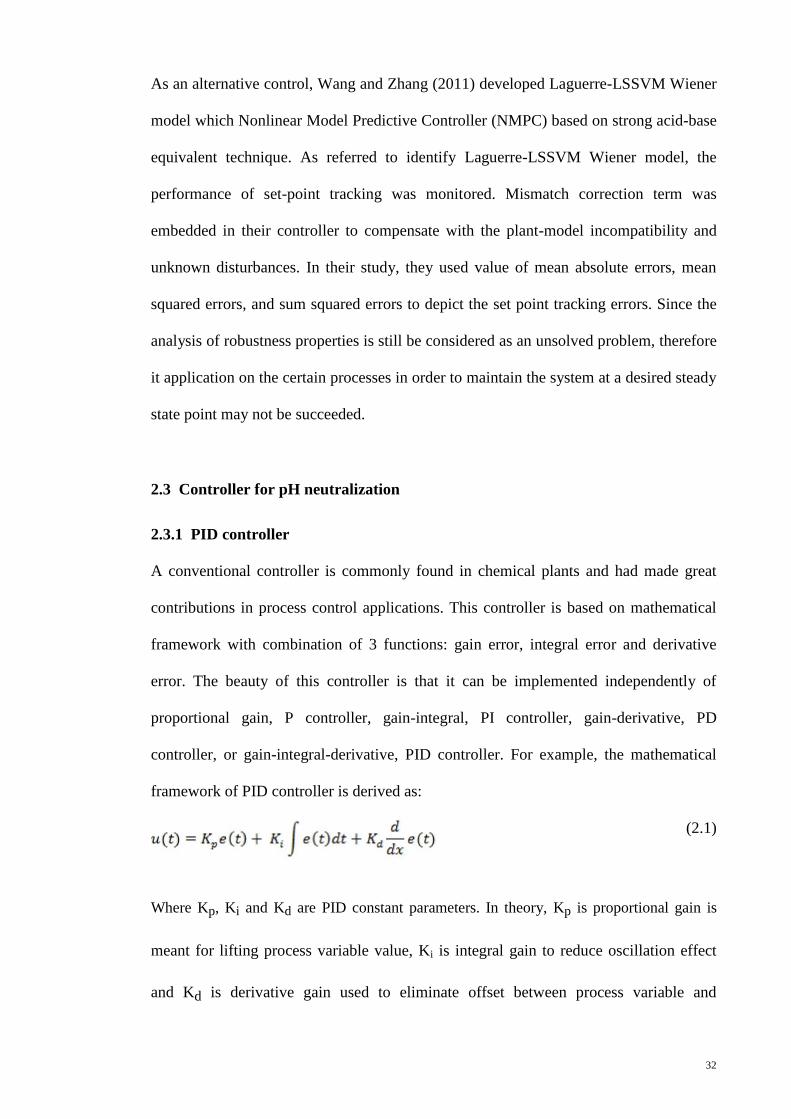
framework of PID controller is derived as:
(2.1)
Where Kp, Ki and Kd are PID constant parameters. In theory, Kp is proportional gain is
meant for lifting process variable value, Ki is integral gain to reduce oscillation effect
and Kd is derivative gain used to eliminate offset between process variable and

33
reference parameter. This combination is one of the earliest control strategy in process
control. It has been tested in many applications and still maintains a good reputation
compared to other controller in literature. A PID controller is commonly used in many
industries nowadays and over 90% of the controllers in chemical industries today are
PID controllers (or at least some form of PID controller like a P or PI controller) .This
approach is often viewed as simple, reliable, and easy to understand. A standard design
method for PID controller can be found in many literatures either from mathematical
formulation or from empirical technique. Establish empirical method like Ziegler-
Nichole can be used to design this controller perfectly. Tuning formulation for PID
parameter also can be found in Cohen-Coon theory.
However, these kinds of controllers have difficulty in handling complex process plant.
This framework is only capable of handling linear process plants, while for nonlinear
system, only at certain region, which has been linearized, could be implemented.
Furthermore, other data except error are ignored because they do not fit into the
mathematical framework in the controller and this valuable information is wasted.
Therefore, the study used advanced controller such as Fuzzy Logic system to control
nonlinear and complex process. Next section described a Fuzzy Logic Controller that
utilizes historical data from the plant and conventional controller it will performs better
control action as in objective control plant.
2.3.2 Fuzzy Logic controller
“As complexity rises, precise statements lose meaning and meaningful statement loses
precision” – Zadeh (1965).
Fuzzy logic controller is widely known among researchers and a lot of findings have
been made in process control applications. The implementation of linguistic variables
like “low” or “high” make fuzzy system favour in many applications either in household
appliances or industrial practice. This controller is used in many ways in control

34
application from simple to complex control system. For instance, Fuzzy Logic was
established ages ago in a washing machine produced by LG, Electrolux and many more.
This application is used to monitor conditions inside the washing machine by using
sensors. By implementing this controller, a machine can adjust setting parameter to
ensure the best performance is achieved. As a result, user can save money by reducing
water and energy as low as possible.
Fuzzy control is established and well documented by Zadeh (1965). Fuzzy Logic system
has inspired researchers and engineers until today. His work is based on formulating a
human language command to a standard set of knowledge based. At initial step, this
fuzzy system requires a set of input and output variables based on the requirement of the
process system known as a membership function. In general, the more variables taken
into the system more precise the controller will be. In contrast, more rules should be
supplied to system and sometime it makes fuzzy system with an abundant of
unnecessary rule. The next step is to determine the type of membership function like
triangular, trapezoidal and many more (see Table 2.1 below for some examples of the
membership function). For example, by using triangular form we can represent large
bounded values normally 0 and 1.
This study designed two types of Fuzzy Logic controller which based on Sugeno and
Mamdani inferences system.
2.3.3 Mamdani type fuzzy logic controller
Mamdani’s type fuzzy inference is the first fuzzy methodology systems establish using
fuzzy set theory. King and Mamdani (1977) has proposed Fuzzy Logic inference to
control steam engine. It has an easy approach to utilize linguistic knowledge in
designing Fuzzy Logic controller. The reasons are that no mathematical equation is
required and it straightforward procedure in mapping knowledge information into a
fuzzy set.

35
2.3.4 Sugeno type fuzzy logic controller
On the other hand, Takagi and Sugeno (1985) , and Sugeno and Kang (1986) proposed a
Sugeno’s fuzzy inference. It’s an equation based and has systematic procedure in fuzzy
design.
Many researchers preferred this fuzzy inference since it can cooperate with
mathematical analysis, adaptive technique, and it is a computational load effectives.
Fuzzy inferences have three similar components between both types above. They are:
1. Membership functions and linguistic variables,
2. Logical operations and
3. Fuzzy rule base, “if-then”.
Membership function (MF) is a linguistic set represented by geometric shape and is
used for a conversion between crisp value and linguistic value. MF is an item inside
input-output variables and it holds properties like name, range, and type. Both type
either Mamdani or Sugeno, used same approaches in defining membership functions
(Emami et al., 2000).
In Fuzzy Logic controller, we can specify as many as membership function in input
variables. However, it will be a burden on controller performance since possible unique
rule is power of number membership function to input variable. Membership functions
for input variables can be selected as in Table 2.1 (Tanaka & Wang, 2002) as shown
below.

36
Table 2.1: Membership functions
Membership Functions Graphical Illustrations
Although there is a lot of membership function types in literature, Table 2.1 shows, the
most commonly found in Fuzzy Logic controller membership functions.
However, Sugeno’s defined fuzzy output variable in mathematical equation form is
different from Mamdani’s approach. In Sugeno’s method, f(x,y) is a polynomial
function in the input variables x and y or constant value. While, Mamdani used same
approaches in defining membership function as in input variables.
Fuzzy logic is known for logical operator like AND, OR and NOT. These operators
actually describe Fuzzy Logic reasoning in general. In Fuzzy Logic controller, this
operator is used as a connector between input and output membership functions. The
purpose of logical expression is to evaluate each membership functions value either 1
(completely true) or 0 (completely false) or range between 0 and 1. For simplicity,
37
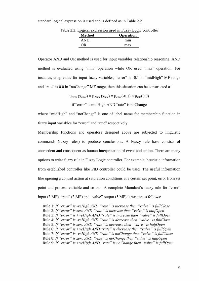
standard logical expression is used and is defined as in Table 2.2.
Table 2.2: Logical expression used in Fuzzy Logic controller
Method Operation
AND min
OR max
Operator AND and OR method is used for input variables relationship reasoning. AND
method is evaluated using “min” operation while OR used “max” operation. For
instance, crisp value for input fuzzy variables, “error” is -0.1 in “midHigh” MF range
and “rate” is 0.0 in “noChange” MF range, then this situation can be constructed as:
µerror (xerror) × µArate (xrate) = µerror(-0.1) × µrate(0.0)
if “error” is midHigh AND “rate” is noChange
where “midHigh” and “noChange” is one of label name for membership function in
fuzzy input variables for “error” and “rate” respectively.
Membership functions and operators designed above are subjected to linguistic
commands (fuzzy rules) to produce conclusions. A Fuzzy rule base consists of
antecedent and consequent as human interpretation of event and action. There are many
options to write fuzzy rule in Fuzzy Logic controller. For example, heuristic information
from established controller like PID controller could be used. The useful information
like opening a control action at saturation conditions at a certain set point, error from set
point and process variable and so on. A complete Mamdani’s fuzzy rule for “error”
input (3 MF), “rate” (3 MF) and “valve” output (5 MF) is written as follows:
Rule 1: If “error” is -veHigh AND “rate” is increase then “valve” is fullClose
Rule 2: If “error” is zero AND “rate” is increase then “valve” is halfOpen
Rule 3: If “error” is +veHigh AND “rate” is increase then “valve” is fullOpen
Rule 4: If “error” is -veHigh AND “rate” is decrease then “valve” is fullClose
Rule 5: If “error” is zero AND “rate” is decrease then “valve” is halfOpen
Rule 6: If “error” is +veHigh AND “rate” is decrease then “valve” is fullOpen
Rule 7: If “error” is -veHigh AND “rate” is noChange then “valve” is fullClose
Rule 8: If “error” is zero AND “rate” is noChange then “valve” is halfOpen
Rule 9: If “error” is +veHigh AND “rate” is noChange then “valve” is fullOpen

38
However, Sugeno’s fuzzy rule can be written as
Rule 1: If “error” is -veHigh AND “rate” is increase then “valve” is f1(x1,x2)
Rule 2: If “error” is zero AND “rate” is increase then “valve” is f2(x 1,x2)
Rule 3: If “error” is +veHigh AND “rate” is increase then “valve” is f3(x 1,x2)
Rule 4: If “error” is -veHigh AND “rate” is decrease then “valve” is f4(x1,x2)
Rule 5: If “error” is zero AND “rate” is decrease then “valve” is f5(x 1,x2)
Rule 6: If “error” is +veHigh AND “rate” is decrease then “valve” is f6(x 1,x2)
Rule 7: If “error” is -veHigh AND “rate” is noChange then “valve” is f7(x1,x2)
Rule 8: If “error” is zero AND “rate” is noChange then “valve” is f8(x 1,x2)
Rule 9: If “error” is +veHigh AND “rate” is noChange then “valve” is f9(x 1,x2)
Where fi(x1,x2) = Ai*x1 + Bi*x2 + Ci and A, B and C are constant parameter in output
functions, fi for i = 1 to 9, while, x1 and x2 is crisp value for error and rate respectively
(Gürocak & de Sam Lazaro, 1994). Unique possible rules that can be generated in both
fuzzy rules are nine since membership functions power to number of inputs.
In process control, Fuzzy Logic system can be used either in process modelling or
process control. In controller perspective, Fuzzy Logic controller is a universal
controller that can be implemented in linear to nonlinear systems. In standard form,
Fuzzy Logic system has four elements as shown in Figure 2.3.
They are:
i. Fuzzification – a process for converting crisp inputs into membership labels in
fuzzy set.
ii. Rule-Base – stored fuzzy rule knowledge in fuzzy set
iii. Inference mechanism – a mapping mechanism for active membership functions
between input, output, and fuzzy rule to produce several conclusions.
iv. Defuzzification – a compilation of active conclusions given by fuzzy inference
system into a single crisp control action.

39
Figure 2.3: Fuzzy Logic controller
In Figure 2.3, a typical Fuzzy Logic controller used in many process control literature is
presented (Filev & Yager, 1994; Maeda & Murakami, 1988; Obut & Ozgen, 2008). In
this study, two inputs and one output are used in our Fuzzy Logic controller and for this
reason; it will be described later in Fuzzy Logic controller design section. Actually, the
number of input and output can be as much as possible depends on control system
requirement. Meanwhile, the Fuzzy Logic controller operation for

40
Mamdani’s type is as follows:
Figure 2.4: Fuzzy Logic controller operation procedure
As seen in Figure 2.4, Fuzzy Logic controller processes the crisp input into control
action as output depending on fuzzy inference defined earlier. The crisp input (x1 and
x2) could trigger any number of rules and gives several conclusions associated with the
membership functions range. Then Fuzzy Logic controller concludes only single crisp
value by defuzzification method. This method indicates a numeric value resulting from
condition in fuzzy inference mechanism and conclusion in rule-base. Defuzzification
represents action taken by controller in individual control loop cycle. Based on

41
Mamdani’s type, there are several defuzzification methods as shown in Table 2.3
(Tanaka & Wang, 2002).
Table 2.3: Mamdani defuzzification method type
Type Mathematical form Graphical form
Centre of
Area
Modified
Centre of
Area
Centre of
Sums
Centre of
Maximum
In Sugeno’s defuzzification method, control action is computed as;
where fi is the output function and wi is the fuzzy rule firing strength for fi that is being
triggered (Tanaka & Wang, 2002). Fuzzy rule firing strength, wi, can be defined as a
combination of fuzzy operator (AND/OR) and input membership functions, µA (A is
error and rate) , and can be written as
wi = AndMethod(µerror(x1), µrate(x2))

42
The motivation on developing the Fuzzy logic controller is because the technique can
give a good performance in controlling complex chemical plant such as fermentation
process, neutralization process and many more. Furthermore, it utilizes human
knowledge rather than mathematical methods, which makes it more close to the system
problem. For this reason, a conventional controller is less attractive than Fuzzy logic
controller because it only satisfies linear process systems and simple plants.
As conclusion, Fuzzy logic control provides a formal methodology for representing,
manipulating, and implementing human’s heuristic knowledge. By implementing this
controller into a process control system, it will minimize error in feedback closed-loop
control system with less overshoot, eliminate offset and reduce oscillation effect.
2.3.5 Neural-Network
Neural network (NN) is an artificial intelligent system replicated from the human brain
neuron concept. McCulloch and Pitts (1943) found neural network concept by
performing mathematical processing of neuron like brain activity. Their concept
represented the activity of individual neurons using simple threshold logic elements, and
showed how interconnected network units could perform the logical operations. Then
Rosenblatt (1962) make a generalization in neuron connection called preceptor, which is
a binary classifier, which map input, x into output, f(x) in artificial neural network
system.
a) Neural network structure
Neural network system consists of several nodes in input layer, hidden layers and
output layer as shown in Figure 2.5 (Nrgaard et al., 2000).
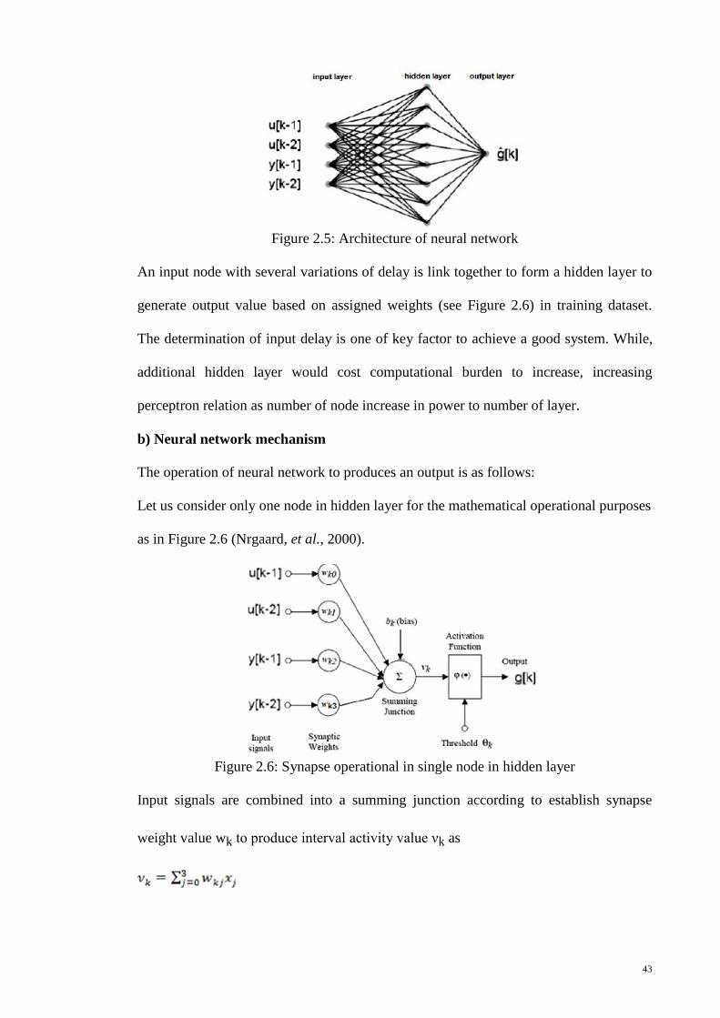
43
Figure 2.5: Architecture of neural network
An input node with several variations of delay is link together to form a hidden layer to
generate output value based on assigned weights (see Figure 2.6) in training dataset.
The determination of input delay is one of key factor to achieve a good system. While,
additional hidden layer would cost computational burden to increase, increasing
perceptron relation as number of node increase in power to number of layer.
b) Neural network mechanism
The operation of neural network to produces an output is as follows:
Let us consider only one node in hidden layer for the mathematical operational purposes
as in Figure 2.6 (Nrgaard, et al., 2000).
Figure 2.6: Synapse operational in single node in hidden layer
Input signals are combined into a summing junction according to establish synapse
weight value wk to produce interval activity value νk as

44
Finally, the output, g[k] is evaluated by some activation function, φ with value of νk
and bias, bk as shows
A threshold function θk could be introduced as an enhancement to the activation
function. The resulting value, g[k] is an input to the output layer to produce final output,
of neural network system and the mathematical operation repeat as explained ĝ[k]
before.
As seen above, every neuron (node) consists of established weight like biological
neuron in human brain. This weight is the so called information of action in the input
system. Thus, training neural network system using input-output dataset is required to
establish weight values to match process system. Additional parameters like desired
output dj and error ej are required to be implemented inside neural network architecture
as shown in Figure 2.7 (Nrgaard, et al., 2000).
Figure 2.7: Neural network learning architecture
Learning operation is to determine wk at every synaptic weight and it can be described
as follows

45
Where, w’jk is previous synapse weight, learning rate (LR), ej is an error between
desired and output value and Xi is input data into neural network. The mechanism of
neural network learning is known as back propagation method and it is the simplest
among available methods in the literature. Detailed information regarding to operational
neural network and training, can be found in open neural network literature.
c) Neural network in control system
Neural network has a great influence in the process control field. Like Fuzzy Logic
system, the framework does not require mathematical representation on process system
as described above. The capability of neural network has excited many researchers in
especially in nonlinear behaviour, time variant problem, and noisy conditions. A
promising performance of accuracy is the key factor why network is most favoured
among other AI systems. A lot of literature can be found regarding neural network
either in process modelling or in control engineering. This technique has benefited
many applications especially in Chemical Engineering field. Hussain (1999) provided
an extensive review of the various applications utilizing neural network technique. In
that article, neural networks are categorized under three major control schemes; inverse
model based control, predictive control and adaptive control methods.
Hussain and Kershenbaum (1999) have succeeded in implementing a neural network
control system for a chemical reactor both in simulation and experiment based. In their
finding, neural network give outstanding performances compared to conventional
control system.

46
2.4 Hybrid system
The hybrid system is a combination of more than one technology used to obtain a
problem solution. It designed to reduce a particular technology limitation and inherit its
advantages. In theory, the hybrid maybe classified into several categories as sequential,
auxiliary, and embedded hybrids (Rajasekaran & Pai, 2004). These classified hybrids
are described based on the interaction of technologies.
The most common interaction between the technologies is using sequential hybrid. The
interaction between first and second technology is a queue-based solution as shown in
Figure 2.8 below. The sub-solution from first technology is transferred to the second
technology, which produces the final solution to the problem.
Figure 2.8: Typical sequential hybrid of two methods
Auxiliary hybrid as in Figure 2.9 is another way to combine two technologies. The
interaction is divided into two parts, which is primary and secondary technology. The
secondary (technology B) is providing an additional sub-solution while a primary
technology is working to produce the final output. This hybrid technique is used
commonly for adaptive control strategy. The controller is being supported by an
approximate algorithm to produce a sub-solution that gives suggestion, while the
controller produces final output for control action.

47
Figure 2.9: Typical auxiliary hybrid of two methods
While, embedded hybrid simultaneously produces sub-solution and the final solution is
managed by technology desired most. This mechanism can be found in the most soft-
computing method where in the method structure is composed of many sub-methods
that gave sub-solution before the final output is compute. Neural-Network, Fuzzy Logic
is one of the soft-computing tools used hardly in this hybrid. The perceptron (for
Neural-Network) or the fuzzy inference (for Fuzzy Logic) is a sub-method which
produces the sub-solution while the fuzzy inference compute the final output by
considering the neuron weight (for Neural-Network) and fuzziness input (for Fuzzy
Logic) in to the summation equation.
Figure 2.10: Typical embedded hybrid of two methods

48
2.4.1 Adaptive Neural Fuzzy Inference System (ANFIS)
ANFIS is a mixture of soft-computing tool between Neural-Network and Fuzzy Logic.
The technology behind this controller is mainly from the Fuzzy Logic system and the
Neural-Network tools for optimizing the configuration of the fuzzy inference system.
ANFIS can be classified as auxiliary hybrid since it uses primary and secondary hybrid.
ANFIS technique has been introduced by Jang (1993) by using Sugeno’s fuzzy system
with neural network method.
Sugeno’s Fuzzy Logic system has the ability to implement mathematical equations in
output function while it embraces all Fuzzy Logic system ability like mapping
nonlinearity, uncertainty and variation over time in complex plant behaviour and fuzzy
knowledge can be obtained from human experience. However, Fuzzy Logic controller
has it drawback. For instance, it is difficult to determine the exact fuzzy rule
relationship and membership functions as complexities of the plant increased.
Furthermore, an extensive effort is needed in describing system behaviour since more
rules are needed to tune accordingly for a good Fuzzy Logic controller.
For neural networks, to find appropriate input and output relationship (perceptron) of
the process is difficult since neural network inner framework is a “black-box” in nature.
In online implementation, neural network is the most expensive cost solution compared
to other technologies. It requires many data in regard to the process, and data used must
represent plant dynamics, and if not, this technique will have trouble in predicting
output. Besides, effective neural network structure is sometime hard to construct when
dealing with a complex system.

49
Thus, a combination of fuzzy system and neural network can improved the problems
related in each technology. Although the main framework of ANFIS is Fuzzy Logic, but
the configuration of Sugeno’s fuzzy inference is prepared by neural network technique.
The neural network technique can be used as a learning mechanism in input and output
dataset. The learning knowledge could be utilized to generate a Fuzzy Logic rules and
membership functions, which conventional Fuzzy Logic may took extra work.
Indirectly, development activity of Fuzzy Logic controller for complex is reduced
significantly.
2.4.2 ANFIS architecture
In general ANFIS architecture has the same components as Sugeno’ type Fuzzy Logic
system with polynomial output function fi(x,y) of input variables, x, y where i is the
number of fuzzy rules used as shown in Figure 2.11 (André Jones et al., 1986).
Figure 2.11: Sugeno’s type Fuzzy Logic system with polynomial output function
Figure 2.12: Equivalent ANFIS architecture to Sugeno’s type Fuzzy Logic system

50
The ANFIS architecture follows the feed forward neural network and is trained using a
supervised learning mechanism. The learning objective is to find the consequent
equation parameters that fit input-output dataset. As shown in Figure 2.16, fis structure
has 5 working layers as briefly described below:
1. Input layer
2. “Inputmf” layer
3. Rule layer
4. “Outputmf” layer
5. Output layer
Layer 1: Input layer – is used to convert crisp value of x and y to label as used in input
membership function. The output of this node, O1 is
O1,I = µAi(x) for i = 1,2 and O1,j = µBj-2 (y) for j =3,4
As described in Chapter 3, input membership function can be selected from several
types (Refer to Table 4.2).
Layer 2: “Inputmf” layer – is used to calculate the weight, wi of relationship
membership functions. The output of this node is relationship weight between input x
and y.
Layer 3: Rule layer – is used to combine consequent action with input relationship. As
from previous layer, this layer works to combine several active rules in fuzzy inference
system and gives output, O3, as total average weight.

51
Layer 4: “Outputmf” layer – is used as an adaptive platform to adjust consequent output
parameter in ANFIS framework. The output, O4, from this node performs consequent
action in each active fuzzy rule.
Layer 5: is used to compute overall output function to final output in ANFIS system
As described above, layer in ANFIS has similar working structure as neural network in
designing fuzzy inference system. The adaptive mechanism works to adjust consequent
constant parameter within several iterations by reducing error between overall ANFIS
output and supplied output data set. Thus, any fitting mechanism can be used to find
consequence parameters, for instance, gradient descent, least squares method, genetic
algorithm, particle swarm or hybrid between those techniques.
2.4.3 Inverse ANFIS model
An accurate technique in connecting the input and output for a process plant is a major
attraction in the ANFIS research. ANFIS is an attractive solution where it allows human
knowledge to be used automatically to determine the control action, u for conventional
Fuzzy Logic controllers. ANFIS provides satisfactory results in dynamic mapping
process plant and this technology can be used in the control plants at any desired set
point. In this study, the ANFIS model is designed to give appropriate control action for
fuzzy logic controller based on the inverse model response where the input and output
relations at online dataset is reversed.

52
Initially, input and output dataset are prepared in open loop plant. In process plant
model identification using ANFIS, input data is a manipulating variable, u and the
output is process variable, y. ANFIS model then is validated in real time to guarantee
the trained model could predict the process variable, y for any given inputs, u. In order
to design an inverse model controller, the dataset is inversed by changing the input
output orientation, for instance, input dataset for ANFIS controller is taken from output
dataset of model, and output dataset for ANFIS controller is from input model dataset.
By doing this inversed dataset, the controller would predict control action, u for any
desired process variable in process control system.

53
Chapter 3 : Modelling of pH
Neutralization process
3.1 Model and controller designs considerations
It is important to specifying control objectives and design considerations beforehand
because it would give a systematic optimized design approach.
The interested parameters are like rise-time, overshoot, and tracking specifications. In
this study, the controller objectives are to achieve less overshoot, fastest rise time, less
oscillation, and reduced robustness affects. To achieve the objectives, several technical
ideas are considered.
First, designed controller must be able to operate for nonlinear process behaviour. This
is very crucial consideration for selected a nonlinear controller. In “Literature review”
chapter, we listed several recent controllers that were used in pH neutralization control-
system. Fuzzy Logic controller is selected since it has the capacity to deal with
nonlinear process behaviour. Detailed description will be given in the next section of
this chapter. The concerned of nonlinearity for pH neutralization is at the set point of
interchange regions. This is because the need of the control action is different. In
neutralization region, a very small control action is required while requiring a large
control action at acid and base regions. This need will give a problem to linear
controllers like PID controller but not for Fuzzy Logic controller.

54
Second, the designed controller must be able to reduce the un-design factor due to aged
plants or altered parameters. This consideration is an optional for many controlled plant
engineers since the controller could be redesigned according to new working
parameters. However, it will be non-economic for the production floor to shut-down and
redesign the controller. Therefore, the designed controller must be able to increase
robustness due to un-design factors as mentions above.
The success of a robust controller is related to the plant dynamic accuracy. Next, model
accuracy is another aspect to achieve in the controller objectives. The designed model
must be able to give accurate prediction of on-line pH value during control system
implementation (at nominal or different working conditions). The robust controller
depends on the accuracy of this model. It is importance to improve the robustness in
Fuzzy Logic controller. Hence, hybrid model is introduced to give accurate model for
on-line prediction.
Other considerations will be discussed in the following sections.
3.2 pH neutralization model designs
This study developed a hybrid model from first principle mathematical model and
Fuzzy Logic model with Neural Network mechanism. The study propose a hybrid
mechanic, which managing the models contribution to achieve best agreement in
dataset. The study designed a pH neutralization model based on Figure 3.1. In the
mixing tank, strong acid (HCl) flow rate and strong base (NaOH) flow rate are mixed
which produced a dynamic behaviour in pH characteristic. The study is to predict the
pH value for this problem by using hybrid modelling.

55
Figure 3.1: Basic design of studied pilot plant
3.2.1 Mathematical model
The mathematical model for pH neutralization process is based on material balances
and chemical equilibrium equation. The model follows McAvoy (1972) and Wright et
al. (1991) works. The mathematical model based is obtained from strong acid
(Hydrochloric) and strong base (Sodium Hydroxide) reaction according to Figure 3.1.
Assumptions for the model are instantaneous reaction, well-mixed, constant-density
mixture, and no formation of solids during experiment. Unsteady-state kinetic model
for pH neutralization is written as in Eq.3.1 below. Where Vr is tank volume, Fa is acid
flow rate, Fb is base flow rate, CA0 and CB0 is a concentration for acid and
base respectively.
(3.1)
(3.2)
Gustafsson and Waller (1983) define Eq.3.2 as the overall-total-ionic-concentration in
mixed tank. The ai(pH) is identified for strong acid as -1, and strong base as +1
(Wright et al., 1991). Thus, x is the remained ionic concentration in the mixture when
acid and base is neutralized where xi is an ionic concentration of reactants.

56
In aqueous solution, mixture of ion hydrogen and Hydroxide is electrically neutral.
Therefore, electro-neutrality and water-equilibrium theories is used to express
electrolyte disassociations (Eq. 3.3) by considering the system is in aqueous solution,
isothermal reaction at temperature 27 oC, and water equilibrium constant, Kw at
1×10-14
(3.3)
Then, kinetic model from Eq. 3.1 can be updated based on hydrogen concentration as
in Eq.3.4.
(3.4)
Eq. 3.4 is a nonhomogeneous and nonlinear differential equation. A numerical tool like
Eular or Runge-Kutta method can be used to solve this equation. The complete pH
neutralization model is gained after solving Eq.3.4 and used that solved value at time, t
into Eq.3.5 in which pH value is calculated by taking the logarithm of hydrogen
concentration, as below:
pHm(t;Fa,Fb) = - log10([H+]) (3.5)
The inputs force that is affecting the pH characteristic is mainly because of the inlet
flow rate. Therefore, in this model, acid (Fa) and base (Fb) flow rates are inputs-signal,
and pH value is the output-signal for the model while the rest are constants. The
nominal operating parameters are referred to in Table 3.1 (Ishak et al., 2001).
Table 3.1: Nominal operating conditions of pH neutralization
Parameter Symbol Value Unit
Acid flow rate Fa 3.5 ± 0.1 litre/min
Base flow rate Fb (5 to 13) ±0.1 litre/min
Initial condition of HCl CAo 0.003 mol/litre
Initial condition of NaOH CBo 0.003 mol/litre
Volume of mixing tank Vr 100 litre
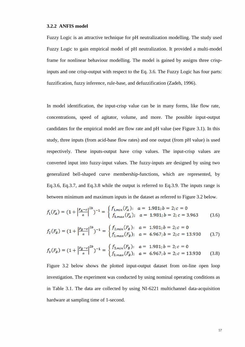
57
3.2.2 ANFIS model
Fuzzy Logic is an attractive technique for pH neutralization modelling. The study used
Fuzzy Logic to gain empirical model of pH neutralization. It provided a multi-model
frame for nonlinear behaviour modelling. The model is gained by assigns three crisp-
inputs and one crisp-output with respect to the Eq. 3.6. The Fuzzy Logic has four parts:
fuzzification, fuzzy inference, rule-base, and defuzzification (Zadeh, 1996).
In model identification, the input-crisp value can be in many forms, like flow rate,
concentrations, speed of agitator, volume, and more. The possible input-output
candidates for the empirical model are flow rate and pH value (see Figure 3.1). In this
study, three inputs (from acid-base flow rates) and one output (from pH value) is used
respectively. These inputs-output have crisp values. The input-crisp values are
converted input into fuzzy-input values. The fuzzy-inputs are designed by using two
generalized bell-shaped curve membership-functions, which are represented, by
Eq.3.6, Eq.3.7, and Eq.3.8 while the output is referred to Eq.3.9. The inputs range is
between minimum and maximum inputs in the dataset as referred to Figure 3.2 below.
(3.6)
(3.7)
(3.8)
Figure 3.2 below shows the plotted input-output dataset from on-line open loop
investigation. The experiment was conducted by using nominal operating conditions as
in Table 3.1. The data are collected by using NI-6221 multichannel data-acquisition
hardware at sampling time of 1-second.
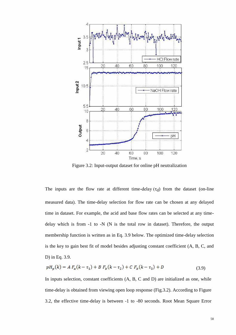
58
Figure 3.2: Input-output dataset for online pH neutralization
The inputs are the flow rate at different time-delay (τd) from the dataset (on-line
measured data). The time-delay selection for flow rate can be chosen at any delayed
time in dataset. For example, the acid and base flow rates can be selected at any time-
delay which is from -1 to -N (N is the total row in dataset). Therefore, the output
membership function is written as in Eq. 3.9 below. The optimized time-delay selection
is the key to gain best fit of model besides adjusting constant coefficient (A, B, C, and
D) in Eq. 3.9.
(3.9)
In inputs selection, constant coefficients (A, B, C and D) are initialized as one, while
time-delay is obtained from viewing open loop response (Fig.3.2). According to Figure
3.2, the effective time-delay is between -1 to -80 seconds. Root Mean Square Error

59
(RMSE) is used as objective function (Eq.3.10 below) to compare the predicted pH
value for ten different time-delay candidates for three inputs.
(3.10)
Where pHr(k) is on-line pH value in dataset from k = 1,2,3 to N, which N is total
number in dataset. The chosen time-delay for τ1 and τ2 (as in Eq. 3.9) is at -72th
and -
73th
seconds respectively for Fb, and for τ3 is at -40th
seconds for Fa. These three inputs
combination gives the lowest value (RMSE = 0.2459) according to Figure 3.3, which
gives the best fit of real data in dataset.
Figure 3.3: Sequential input selection for three inputs from 10 candidates
The rule-base for the model is composed by taking maximum relationship among three
inputs. The rule-base is eight unique logical combinations that are from 3 inputs and
two membership functions (23). The rules are listed as in Table 3.2.

60
Table 3.2: Eight unique combinations among inputs and output for fuzzy rule-base
AND Input2 is f2,min(FB-72) AND Input2 is f2,max (FB-72)
AND Input3 is f3,min(FB-73) AND Input3 is f3,min(FB-73)
If Input1 is f1,min(FA-40) Rule#1 : then output is pH1(k) Rule#2 : then output is pH2(k)
If Input1is f1,max(FA-40) Rule#3 : then output is pH3(k) Rule#4 : then output is pH4(k)
AND Input2 is f2,min (FB-72) AND Input2 is f2,max (FB-72)
AND Input3 is f3,max(FB-73) AND Input3 is f3,max(FB-73)
If Input1is f1,min(FA-40) Rule#5 : then output is pH5(k) Rule#6 : then output is pH6(k)
If Input1is f1,max(FA-40) Rule#7 : then output is pH7(k) Rule#8 : then output is pH8(k)
The fuzzy-output is linear functions consisting of fuzzy-input membership function.
Eq.13 can be elaborated to eight different cases as Eq.3.11
(3.11)
where i = 1,2 to 8
The coefficient function (Ai, Bi, Ci and Di) are the gains that are needed to be optimized for
best fit of pH neutralization dataset. The complete construction of fuzzy model can be
seen at Figure 3.4, which have three parts (input, rule, and output) as describes in Fuzzy
Logic.
Figure 3.4: ANFIS model structure

61
Figure 3.4 shows likeness to ideas in Neural-Network (N-N) architecture (see Section
2.3.4). In N-N, input-signals are combined at summing junction and the node output
(internal-activity value) is calculated by multiplying the synapse weight value for each
signal respectively. In neuro-fuzzy case, synapse weight is the coefficient (Ai, Bi, Ci,
and Di) while the summing junction is at Eq.15 which combines the active rule-base
with the synapse weight at each fuzzy-inputs to produce a crisp output-value (pHp(k)).
As in Neural-Network identification, neuro-fuzzy have to train the synapse weight
with the on-line dataset (Figure 3.2). Least-square method (learning algorithm) is used
to get the optimized synapse weight (Ai, Bi, Ci, and Di) by iteratively reducing the
cost of objective function (Eq.14) for entire fuzzy-structure (Table 3.3Table 3.3)
Table 3.3: Optimized coefficients of ANFIS output-function
i Ai Bi Ci Di
1 0.3524 0.5574 0.03086 0.167
2 1.073 0.06756 -0.006016 -0.1915
3 -0.05421 1.057 -0.5296 0.9288
4 1.337 0.4237 0.3674 -9.853
5 0.8138 -0.4955 0.4823 4.041
6 1.255 0.1555 -0.2992 0.7469
7 0.7408 0.2627 0.0578 0.1502
8 0.1921 0.7397 0.05951 -0.2554
The final layer (control output) gives a value by summing all conclusion values. It
is described as
(3.12)

62
3.2.3 Hybrid ANFIS and mathematical model
A hybrid is also known as a combination of several techniques. This study used two
different techniques, which is a combination of mathematical model and empirical
model. Lennart (2010) classified the hybrid model as in “slated grey” colour analogy,
with a combination of first principle model (“pure white”) and soft computing model
(“black”).
Let us consider the dynamic continuous time mathematical model and empirical model
as in Eq.3.5 and Eq.3.12 respectively as below.
(3.13)
(3.14)
The mathematical model (Eq.3.13) is a typical physical first order continuous time
domain model which presenting Eq.3.5. Next, Eq.3.14 is an empirical model
constructed by historical dataset based on a modelled plant that present 3.12. Both
models have different mechanics in predicting the response of the plant. Mostly,
Eq.3.13 represents a theoretical formulation and Eq.3.14 is on identification from best
fit of dataset. This study proposes a hybrid mechanic that can combine both methods
and give better dataset agreement compared to standalone model. This study proposes a
two hybrid mechanics which suitable for combining the mathematical and empirical
model.
First is a parallel hybrid that is managed by hybrid weight, α as in Eq.3. The
summation of output weight is always equal to one if and only if α is in range of zero
to one.
(3.15)

63
The yh1(t) is output for hybrid model from combination of Eq.3.13 and Eq.3.14. The
structure is simple and fast. The hybrid weight (α) can be a constant or function, which
the value, leading the prediction toward the theoretical idea or training model. Thus, it
has a capacity of predicting the process-output value within its robustness limitation.
Second, the proposed hybrid structure is constructed by using model performance
weight of individual model. The hybrid model output is calculated as in Eq.3.16 where
the individual output is evaluated according to their performance weight, ω.
(3.16)
The structure above is for combining several models. Every ith
model has been
assigned to a performance weight (ωi) that can be a constant or a function. Eq.3.16 is
more flexible in managing the output contribution because the summation of weight
can be greater that one.
The proposed hybrid structures above can be treated as a static or dynamic equation
depending on its weight. Static equation is from a constant weight while, the dynamic
equation is depended on the functions used. The function can be implemented from on
dynamic equation. Furthermore, proposed hybrid structure can used as on-line adapting
gain for adaptive controller studies. However, the adapting mechanism requires
additional algorithms to perform a dynamic adjustment in on-line basis.
The individual models have several advantages and disadvantages. The ANFIS model
is used to predict the pH value based on the real plant characteristics, while the
mathematical pH model is used to calculate the theoretical pH values. ANFIS duplicate
the dynamics of a pH plant, which depends on training dataset (Figure 3.2). The motive
of introducing the mathematical and ANFIS model is to give better pH value

64
prediction. Subsequently, the hybrid model would extent the robust properties from
nominal working condition. The variations are acid and base concentrations, reactor
volume, mixing agitator speed, unknown compositions, and many more during on-line
implementation.
The hybrid models (Eq.3.17 and Eq.3.18) for pH neutralization are designed by
combining Eq.3.5 and Eq.3.12. Both models are considered in discreet time domain
which sampling time (h) is one second as in dataset (Figure 3.2).
(3.17)
or
(3.18)
Where, for two models, the weight can be written as
and
Thus, the hybrid model design can be seen as
(3.18)
Weight (α) is proportion to each model to predict the output. As mention, the weight can
be selected from a constant number or function. Figure 5 indicates the influence strength
between mathematical and neuro-fuzzy model. The RMSE for hybrid model increased
with increments of the weight (α). This correlation shows that the hybrid model is
influenced by both models, which at nominal condition, neuro-fuzzy model gives better
prediction (less RMSE), compared with the mathematical model (high RMSE).

65
Figure 3.5: Hybrid model RMSE values with different weight selection
The weight (α) equal to zero means that the hybrid model is completely influenced by
neuro-fuzzy model, while the weight when
is equal to one means that the hybrid model is totally influenced by the mathematical
model. These two cases give a correlation to decide the best weight at a particular time
for hybrid model to achieve lowest RMSE. Thus, the weight is selected from time to
time resulting in a dynamic weight profile. Eq. 3.19 is used to assign the dynamic
weight as a function of absolute error from two models (Math and Neuro-fuzzy) since
absolute error shows the magnitude of error deviated from the on-line dataset.
As conclusion, the hybrid model predicts pH value based on performance of
mathematical and neuro-fuzzy model. Selecting best weight from each model will give
good prediction of hybrid model with lowest RMSE. In nominal working condition, the
lowest weight is preferred since neuro-fuzzy model predicts better than mathematical
model. However, when working at new condition, neuro-fuzzy may not perform well.
(3.19)

66
Then, a right weight, is used to compensate for the neuro-fuzzy limitation.
Therefore, the dynamic weight (Eq.19) could select the appropriate weight, which
calculates by deviation magnitude from on-line dataset with models output.

67
Chapter 4 : Controllers design for pH
neutralization process
4.1 Conventional PID controller design
Conventional PID controller has standard mathematical expression. It is a combination
of Proportional action, Integral action and Derivative action as in Eq. 4.1. As describe in
Literature Review section as,
(4.1)
The PID controller design has many methods to follow. This study used industrial
practical method for controlling pH at 7. Since PID controller is only for linear
processes, therefore the design configuration only works around pH 7.

68
The design is follows;
Figure 4.1: PID controller tuning

69
The PID controller has been tuned according to on-line control performance by using
step in Figure 4.1. The tuning parameter can be obtained as in Table 4.1. The
methodologies of conducting those controllers tuning are not described in details. One
can found in many literatures about those tuning method.
Table 4.1: PID tuning parameters
PID controller P I D
Try and error tuning 0.002 12 5
Ziegler-Nichole Tuning
Cohen-coon Tuning
4.2 Fuzzy logic controller design
Fuzzy Logic (Fuzzy Logic) controller design and analysis is discussed in this section.
Fuzzy Logic Controller is described as a decision-making system that works in the
linguistics framework. Fuzzy Logic was been introduced by (Zadeh, 1965), a founder of
fuzzy set theory. In daily activities, fuzzy logic has been practised idea without realizing
it. In conventional fuzzy system, fuzziness has average of 0 to 1. However, in Fuzzy
Logic controller, it has ranges from 0 to 1 and it has systematic approaches that different
from conventional fuzzy idea.
Fuzzy Logic system has a framework called fuzzy inference system (fis) based on
Zadeh fuzzy set. It is a fuzzy methodology for mapping linguistic knowledge into fuzzy
set systems. In Fuzzy Logic controller, fis framework is used to map input signal into
linguistic labels such as “error”, “rate” etc. and evaluate output label depend to
consequent action into crisp value know as control action. Fuzzy Logic system used
human experience information, as knowledge regarding open loop characteristic on pH
modelling from previous section.

70
4.2.1 Fuzzy Logic control strategy
Feedback control strategy is desired for all applications control system in this study. In
feedback loop control (in Figure 4.2), error variable is normally used as a Fuzzy Logic
input. This variable is an essential parameter for guiding the controller to achieve the
desired set point. In theory, “error” is defined as difference between reference value, r(t)
to process variable value, e(t) = r(t) – y(t).
Figure 4.2: Feedback closed loop system with Fuzzy controller.
In addition, error could be extended into rate of error. Since human understand literally
how fast error changes from certain point to another point, rate of error (“rate”) is
another state of Fuzzy Logic input that is interesting to study in the feedback control
system. Label “rate” is defined as change of error in time, rate (t) = d/dt [e(t)]. It is also
known as a gradient of error; either error is increasing or decreasing from previous
state. Thus, these terminologies like “error “and “rate” are used in this strategy. Then,
input label for the Fuzzy Logic controller is chosen as “error” and “rate”.
While Fuzzy Logic controller output (u) can be from any state variables like current,
voltage, flow rate, heat supplied and many more, but it should be related to manipulated
variable in control system. The opening-valve as controller output (manipulated
variables) is used since the opening is a function of flow rate in pH neutralization
control system. In the pilot plant, opening-valve depends on voltage supplied into a
valve transducer. It will convert the voltage to air pressure in psi. Range o to 10miliVolt
is applied for 0% open to 100% open respectively. Therefore, voltage is selected as
output state in Fuzzy Logic controller by using “valve” label.

71
4.2.2 Selection of input and output membership functions
Feedback control system is applied in this study, then “error” is the first item in Fuzzy
Logic controller. The error signal is the same as input in PID controller and for Fuzzy
Logic controller; error is mapped into linguistic variables like “zero”, “negative” and
“positive” for minimal number of fuzzy membership. Three labels are sufficient to map
all bounded error signal from control system. While second input is “rate”. It could be
label as “increased”, “noChange” and “decreased” minimally. However, number of
label (membership) in first input (error) and second input (rate) could be more that
suggested number. It could give more computational load but smooth controller
performance.
The output from Fuzzy Logic controller (“valve”) is divided into 5 labels (membership)
which is “closed”, “smallOpen”, “midOpen”, “largeOpen”and “FullOpen”. It is because
flow rate value (litre/min) between each labels (example: “closed” and “smallOpen”)
has almost no significant difference.
Design of Fuzzy Logic controller is begun by letting data set, Ai and crisp value, xi
(“error”, “rate” and “valve”) into control system. In classical mathematical form, it
might be expressed as:
Aerror
= (xerror
| -1< xerror
< 1) , Arate
= (xrate
| -1< xrate
< 1) and Avalve
= (xvalve
| 0< xvalve
< 10).
However, in fuzzy inference system, data set Ai has an extension to classical data set
which includes each crisp value xi into MF equations for all elements in Ai. This
membership function equations map each element in Xi (Xi is crisp value for all ranges
in MF) into membership value between 0 and 1 as shown below:
Aerror = (xerror, µAerror (xerror) | xerror ∈ Xerror)
Arate = (xrate, µArate (xrate) | xrate ∈ Xrate) and
Avalve =
(xvalve, µAvalve (xvalve) | xvalve ∈ Xvalve).

72
where µAi is MF equation of label represented by a geometrical shape. As initial design,
triangular shape as input MF is used to convert crisp input value by using function
below (µAerror (xerror),µArate (xrate)):
Where a, b, c is triangular shape parameters and i denote as “error” and “rate”. All
graphical MF shape and parameter for inputs variable can be obtained below (Figure 4.3
and Table 4.2) respectively. Triangular shape is favoured initially, because it easy to
construct and gives good performance.
(a)
(b)
Figure 4.3: Graphical illustration of inputs membership function;
(a) input variable “error” (b) input variable “rate”

73
Table 4.2: MF input variables parameter and values.
Name i = “error” i = “rate”
Range Min: -0.5; Max: 0.5 Min: -0.1; Max: 0.1
No Name a b c Name a b c
1 -veHigh -0.8 -0.5 -0.1 increase -0.18 -0.1 -0.02
2 -veMid -0.2 -0.1 0 noChange -0.08 0 0.08
3 Zero -0.01 0 0.01 decrease 0.02 0.1 0.18
4 +veMid 0 0.1 0.2
5 +veHigh 0.2 0.5 0.8
Input “error” contains 5 MF functions where “-veHigh” and “+veHigh” are catered to
cover up error value if pH values reference change from 6 to 8 or vice versa. “-veMid”
and “+veMid” is for converting error value in small scale. While at “Zero” label, the
controller output value should be maintained because the crisp value at moment shows
that the Fuzzy Logic controller has achieved the control objective. On the other hand,
only 3 MF are required for input “rate”. It is minimal number of action since basic rate
can be either increase, decrease or no change.
Figure 4.4 shows the procedure to design the MF as described above.
Figure 4.4: Membership function design procedure
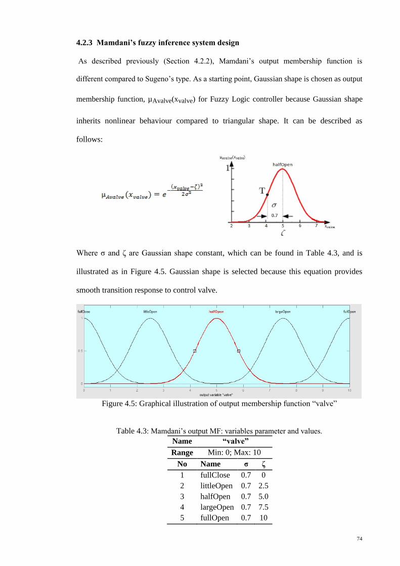
74
4.2.3 Mamdani’s fuzzy inference system design
As described previously (Section 4.2.2), Mamdani’s output membership function is
different compared to Sugeno’s type. As a starting point, Gaussian shape is chosen as output
membership function, µAvalve(xvalve) for Fuzzy Logic controller because Gaussian shape
inherits nonlinear behaviour compared to triangular shape. It can be described as
follows:
Where σ and ζ are Gaussian shape constant, which can be found in Table 4.3, and is
illustrated as in Figure 4.5. Gaussian shape is selected because this equation provides
smooth transition response to control valve.
Figure 4.5: Graphical illustration of output membership function “valve”
Table 4.3: Mamdani’s output MF: variables parameter and values.
Name “valve”
Range Min: 0; Max: 10
No Name σ ζ
1 fullClose 0.7 0
2 littleOpen 0.7 2.5
3 halfOpen 0.7 5.0
4 largeOpen 0.7 7.5
5 fullOpen 0.7 10

75
In pH neutralization control case study, the final element of the control system is control
valve and it ranges between 0 to 10 millivolt crisp inputs value. As in a real-plant,
interval of 2 millivolt is significant opening different for base flow rate to take action.
For instance, 2.1milivolt has no significant change in base flow rate compared to
4milivolt. The next step for Fuzzy Logic controller design is to construct the control
command rules based on input and output MF defined earlier. Fuzzy rules for
Mamdani’s inference system are:
Rule 1: If “error” is -veHigh AND “rate” is increase then “valve” is fullClose
Rule 2: If “error” is zero AND “rate” is increase then “valve” is halfOpen
Rule 3: If “error” is +veHigh AND “rate” is increase then “valve” is fullOpen
Rule 4: If “error” is -veHigh AND “rate” is decrease then “valve” is fullClose
Rule 5: If “error” is zero AND “rate” is decrease then “valve” is halfOpen
Rule 6: If “error” is +veHigh AND “rate” is decrease then “valve” is fullOpen
Rule 7: If “error” is -veHigh AND “rate” is noChange then “valve” is fullClose
Rule 8: If “error” is zero AND “rate” is noChange then “valve” is halfOpen
Rule 9: If “error” is +veHigh AND “rate” is noChange then “valve” is fullOpen
In the list of fuzzy rules above, Rule #8 is the most important since it guaranties the
Fuzzy Logic controller to meet the desired control objective. Determination of the fuzzy
rules can be hard for a new plant but it is easy for an established plant since stationary
state and dynamic response of the plant are available during plant operation. At the pilot
plant, to achieve stationary state (error is zero and rate in not change), flow rate of
NaOH must be the same as HCl flow rate, since both concentration is the same at feed
storage tank. Rule #8 only caters at stationary state with maintain reference and process
variable value.
The rest of fuzzy rules listed above is to drive the process variable (pH) to the desired
reference point. It has two conditions when process variable is below (error is positive)
and above (error is negative) reference value. When error is positive, the mixing tank
requires more NaOH so the action is to increase the opening valve. Another case when
error is negative, the valve opening has to reduce in order to lessen the pH value in tank.

76
4.2.4 Sugeno’s fuzzy inference system design
The designed fuzzy inference system for Sugenno’s method is described in this sub-
section. As continuity from the previous Fuzzy Logic controller design, there are no
changes in input and output definition. As mentioned (Section 4.2.2), Sugenno’s fuzzy
inference for output membership functions has a different approached. Recall that,
Fuzzy Logic controller has five output labels, “closed”, “smallOpen”, “midOpen”,
“largeOpen”and “FullOpen”. In Mamdani’s fuzzy inference, those labels are
represented by geometrical functions. For simplicity, a constant value is used for
Sugeno’s fuzzy inference instead of mathematical equations. In this study, the
designed parameter for Sugenno’s type fuzzy inference can be found in Table 4.4
below.
Table 4.4: Sugeno’s output MF: variable parameters and values.
Name “valve”
Range Min: 0; Max: 10
No Name Value
1 fullClose 0
2 littleOpen 2.5
3 halfOpen 5.0
4 largeOpen 7.5
5 fullOpen 10
Next step after membership design is constructing the fuzzy rule base. Since Mamdani’s
inference has been designed earlier and the process is same, thus the relation for rule
before can be used to complete the fuzzy inference design for Sugenno’s type. The rules
are:
Rule 1: If “error” is -veHigh AND “rate” is increase then “valve” is 0.0
Rule 2: If “error” is zero AND “rate” is increase then “valve” is 5.0
Rule 3: If “error” is +veHigh AND “rate” is increase then “valve” is 7.5
Rule 4: If “error” is -veHigh AND “rate” is decrease then “valve” is 0.0
Rule 5: If “error” is zero AND “rate” is decrease then “valve” is 5.0
Rule 6: If “error” is +veHigh AND “rate” is decrease then “valve” is 10.0
Rule 7: If “error” is -veHigh AND “rate” is noChange then “valve” is 0.0
Rule 8: If “error” is zero AND “rate” is noChange then “valve” is 5.0
Rule 9: If “error” is +veHigh AND “rate” is noChange then “valve” is 10.0

77
4.3 Fuzzy Logic controller with ANFIS Model
4.3.1 ANFIS model design consideration
The motive to implement ANFIS in control system is to increase the quality of Fuzzy
Logic controller.
It can be achieved by using a hybrid technique between model identification and Fuzzy
Logic controller. The inverse mathematical model and inverse ANFIS model is used.
The interaction between these two techniques is auxiliary hybrid (as in Literature
review chapter Section 2.3.4). In this hybrid, the primary technique (Fuzzy Logic
controller) works to produce control-action by using sub-solution from secondary
technique (inverse ANFIS model). The Fuzzy Logic controller is extended by adjusting
the output membership function with sub-solution from inverse ANFIS model. Figure
4.6 shows the close-loop block diagram where inversed hybrid model is supplying the
suggested control action to the Fuzzy Logic controller.
Figure 4.6: Proposed controller in feedback control of pH neutralization plant

78
4.3.2 Inverse ANFIS model design
Fuzzy Logic with combination of ANFIS is an attractive technique to model pH
neutralization. It is because it provides a multi-model framework for modelling
nonlinear behaviour at different pH neutralization regions.
This subsection is an extended step after ANFIS model identification as described at
previous sub-section. The inverse ANFIS model is designed by using same input-output
dataset as in model identification. However, input and output orientation in the dataset
is inversed where the input is pH value and the output is control action. As a result,
ANFIS produces an inverse behaviour of titration curve.
ANFIS training procedure is carried out as usual in ANFIS model identification. The
ANFIS architecture with three inputs and one output is desired to cover control action
dynamics during process control. The inputs are pH values at two different delays and
previous control action at time b is another input variable. While, the output of this
inversed ANFIS model is a predicted control action in millivolt.
Three input groups are chosen for ANFIS model which group no. 1 and 2 are for
previous output value, y(t-1), y(t-2),y(t-3) and y(t-4) and input no 3 is for control valve
input signal u(t-1), u(t-2), u(t-3) to u(t-6). After input is identified, 10 input candidates
are trained and checked by comparing selected delays with input-output dataset for
three iterations and best-fit RMSE for three inputs are known. Delay selection of inputs
is based on lowest root mean square error (RMSE) within three input groups as shown
in Figure 4.7.

79
Figure 4.7: Sequential input selection
Selected inputs are y(t-1), y(t-3), u(t-1) with RMSE training = 0.2255 and RMSE
checking = 0.2729. Inversed ANFIS model as shown in Figure 4.8 has five components
consisting of three input variables, two membership functions in each variable, and
eight unique possible combinations of fuzzy rules, consequent output equation, and
output variable.
Figure 4.8: inverse ANFIS model structure

80
4.3.3 Inverse hybrid model design
The design used a combination of inversed model from first principle and ANFIS.
Hybrid structure below is in a parallel configuration which is known as embedded
hybrid as shown in Figure 4.9. The inversed ANFIS model is used to estimate control
action for a pH value of real plant and inversed pH model is for calculation of control
action of pH value as theoretical basis. ANFIS has capabilities to replicate the dynamics
of inverse pH plant. By introducing mathematical model parallel to the ANFIS, the
inversed model will be more robust in choosing different acid flow rate during
offline/online process control investigation. Furthermore, additional variations like
concentration of acid/base and reactor volume could be captured in the proposed
controller.
On the other hand, hybrid weight α is introduced for managing output contribution of
each model. The range of 0 to 1 for α is used to determine which model contributes
more to the hybrid model. A key success to this model depends on ANFIS prediction
value and hybrid weight, α, parameter as described.
Figure 4.9: Inversed hybrid model structure

81
4.3.4 Hybrid Fuzzy Logic Controller design
Intelligent controller that is being proposed in this study composed of hybrid inversed
model and Sugeno’s Fuzzy Logic controller as shown in Figure 4.10. Auxiliary hybrid
is used to combine both techniques to produce a hybrid intelligent controller that has
ability to adapt and react within allowable plant modification and disturbance.
Figure 4.10: Proposed hybrid controller block diagram
Sugeno’s Fuzzy Logic controller used in this study consists of one input and one output
system. Input membership has three membership functions, which is a minimum
membership function that can be used for feedback loop control strategy.
Figure 4.11: FLC Input membership functions

82
Figure 4.11 shows the input MF (error) label and value used in Sugeno’s Fuzzy Logic
controller while, output variable is a constant value and is labelled as “open”, “good”
and “close” respectively. Open and close can easily be selected since it a boundary of
control action. However, “good” condition depends on steady state of the process when
error is zero. Hybrid inversed model is acted would give a prediction of “good” value at
particular time within a specific control system conditions.

83
Chapter 5 : The pH neutralization
experimental setup
5.1 Control System Setup
5.1.1 Pilot plant design consideration
A good pilot plant design is important to achieve good control performance. In pH
neutralization, to reduce time delay is important since this would create instability in
model and control system. The time delay may be present at process time delay (tank
size), delivery of reagent (acid and base), and measurement device (at pH electrode).
These delays can be minimized if pilot plant is designed properly.
Another importance issue is sensitivity of the final-element (control valve). This is
because at neutralization region it needs a very small control action that require small
amount of reagent to pass through control valve. The proper control valve selection
during pilot plant design could give better quality of control performance.
Next, the environmental issue regarding the pilot plant effluent. The effluent from this
plant must be treated before it passes through to public drain.

84
5.1.2 pH neutralization pilot plant
The neutralization pilot plant is located at Chemical Engineering Department,
University of Malaya. Figure 5.1, show process, and instrument diagram which
illustrate the experimental setup.
Figure 5.1: Process and instrumentation diagram for pH neutralization
It has 500-liter holdup capacity in mixing a rector and 200-liter initial feed supply for
acid and base (Figure 5.2).
Figure 5.2: Pilot plant for pH neutralization

85
The mixing tank design and layout is important as described in Figure 5.1. Our tank has
two inlets flow and four outlets located in the tank. The mixing tank has a recycle
stream which provides a well-mix solution. The outlets stream is mainly to the
discharge the mixture in the tank. One located at the bottom of the tank for
maintenances purpose while the rest located at the side of the reactor vertically. The
height of holdup volume in the reactor is depending on the vertical outlet. The outlets
diameter is much bigger than the inlet diameter so it can guaranty that the height is
always constant at desired level.
The experiment used 100-liter as a holdup volume. It is desired at this level since the
recommendation to have a good mixing condition is when liquid depth is equal to tank
diameter. The reason is to minimize the traveling distant for reagents from the inlet. The
retention time for 100-liter is 7 min that is calculated from volume divided by the flow
rate. In normal practice for liquid-liquid reaction without solid formation, the retention
time (dead time) is from 5 to 20 minutes (McMillan & Cameron, 2005).
The high-speed axial mixing propeller is used at 25 rads per minute (rpm). It is to
reduce the dead time effect and enough to break the fluid inside the tank. So that the
reagent goes to the bottom of the tank since the pH electrode is located at the bottom of
the tank. The dead time td, is 0.32min gained from holdup volume divided by the
summation of inlet flow rate and agitator pumping capacity as shown below.
Table 5.1: Mixing tank details
Parameter Value Unit
Diameter 100 cm
Height 500 cm
Impeller speed 25 RPM
Impeller diameter 9 cm
Baffle 4
Impeller 3 blades butterfly type
Flow rate 9 - 14 Litre/min

86
At the tank, static mixer (Figure 5.3) is installed. The purpose of this mixer is to reduce
dead time delay caused resident time distribution. In literature, the static mixture
reduces 80% of resident time (McMillan & Cameron, 2005).
Figure 5.3: Static mixture for acid and base before entering the reactor
5.1.3 pH sensor
The pH value is measured by pH electrode. The pH value is obtained when pH-sensitive
glass having contact with the aqueous solution. Nerst equation is used to calculate the
potential energy generated from the exchange of hydrogen ion (proton) between
hydronium ions in aqueous solutions.
The pH electrode used is from EUTECH instrument hardware. It is located at the
bottom of the reactor tank. As in Figure 5.4, pH value is obtained inside the mixing
solution, which reduced transportation lag.
Figure 5.4: pH transmitter used in the pilot plant

87
The sensor location is important for pH neutralization control system. It should be
located at most representative, reliable, and fastest measurement. In our experimental
setup, it is located at close to the exit pipe line of the mixing reactor. In this case, the pH
electrode can measure the pH value and the reagent has sufficient time to completely
mix before discharge so that it will increase the controller and model performance.
5.1.4 Control valve
The range-ability for final element is most importance. It determines the controller
performance since pH neutralization has non-sensitive and sensitive control action. In
literature for normal strong acid and base, metering pump should in ratio 20:1 to 200:1
for control action over flow rate (McMillan & Cameron, 2005). In addition, linear valve
characteristic is preferred and using smart digital positioner is recommended.
Figure 5.5: Control valves (acid and base) used in the pilot plant
In the experiment, two units of control valve are used as in Figure 5.5. Both control
valves used is pneumatic type, which require air to open and to close. The transducer is
located near the control valve to convert the control action from millivolt to psig.

88
5.1.4 Control system
The set point change is important. The pH response depends on the regions in titration
curve. Local linear behaviour would be expected if the set point at the flat portion of the
regions. However, the nonlinear controller must be used if the set point is located at two
different regions due to sensitive and non-sensitive control action.
Figure 5.6: Closed-loop structure for on-line study
The tracking specifications depend on process plant requirement as in Table 5.2.
Table 5.2: Control objectives for set-point tracking regions
pH neutralization region Process variable Tracking range
Acid pH 4.5 to 6.5
Neutralization pH 6.5 to 7.5
Base pH 7.5 to 10.5
As in Table 5.2 above, pH neutralization control system, range between 6.5 and 7.5 is
desired since neutralization point is within this range.
The controller in feedback control system is to reduce error between plant and reference
value. Figure 5.7 below shows a control system strategy used in this study.

89
Figure 5.7: Structure of closed-loop block diagram for on-line pH neutralization system

90
5.2 Experimental work procedures
5.2.1 Open loop study
The focus of this section is to describe the steps that being carried out in open loop
experiment. The dynamic profile of neutralization can be obtained through these steps.
The experiment starts with preparing the feed tank as in nominal operating condition
(Refer Table 3.1). At this step, there are no flows for both input streams. It can be done
by sending 0 milivolt to the control valves through control system user interface. On the
other hand, the mixing reactor has to be maintained at 25 rpm agitation speed and
recycle pump is switching on. The open loop study should begin with pH value of 3
(same pH value as in HCL feed tank) and it end at pH of 11 (same pH value as in NaOH
feed tank).
Next, open the HCL stream line control valve about 10% opening. This valve will give
the mixing reactor in acid condition. After sometime, gives step change input of 0 to
100% opening to NaOH stream line control valve. This step will increase the pH value
in mixing reactor. Observe and monitor the pH changes by plotting a real time signal by
using software interface in computer. The open loop study finish when pH value in
reactor saturated.
This open loop procedure has to be repeated at different input step change according to
objective of the investigation. The need to repeat this procedure is must if the data is
used as a training dataset in modelling identification.

91
5.2.2 Closed loop study
As discussed previously, closed loop study is a feedback control system. It has a
complete control system block and it objective is to bring the present value to a desire
set-point value. The objective can be achieved by design the controller appropriately
according to the pH neutralization plant condition and control strategy used.
The procedure in this section can be used for a several closed loop control system
investigations which is carried out in this research. At preliminary step, the plant should
be in a close loop mode and plant condition should be at nominal condition (refer Table
3.1). This step can be checked by verifying the signal at the control panel with the
computer interface. Firstly, bring the mixing reactor at saturation pH value by setting a
set-point block at user interface. Next, the study performs a controller investigation like
servo (set-point change) and regulatory (disturbance rejection) case study.
For servo case, acid stream line control valve should be maintained as in Table 3.1. The
reason is because, for a servo case, we need to see the effect of set-point change only
and by maintaining the flow rate of acid, the deviation of disturbance is equal to zero.
The servo case starts with several set-point changes as described earlier.
For regulatory case, it start when pH value for the mixing reactor at saturation. The
disturbance should be introduced at this state. In this study, the disturbance can be
introduced by changing the acid flow rates differ from the nominal condition.
This study ended by obtains the real-time profiles.

92
Chapter 6 : Result and Discussion
6.1 Models validation
6.1.1 Mathematical model
The mathematical model derived gives “s-shape” curve, which is determined by
logarithm function. In Figure 6.1, the designed mathematical model produced a
characteristic of pH neutralization. It shows the model is nonlinear with several
dynamic regions. At first region (pH < 6), slow response is observed while very fast
response at second region (6<pH<8). At third region, slow response is detected and the
pH is saturated at pH 9.6.
Figure 6.1: Mathematical model profile of pH neutralization (RMSE = 0.7365)
The profile draws a theoretical boundary along the titration curve (same dataset as in
neuro-fuzzy model). Figure 6.1 shows that the mathematical model is able to give pH
value with RMSE = 0.7365. The model using on-line data (signal from acid-base flow
rate) is fed into the model equation. The deviation of theoretical profile with real
experimental profile maybe cause of the assumption made in theory development. It

93
shows an offset but it enough to show the profile is in sigmoidal curve which is basic
theory of strong acid and strong base neutralization.
6.1.2 ANFIS model
The on-line dataset was obtained by fixing the acid flow rate at (5.0 ± 0.1) litre/min and
introducing a step change from (0 to 13.0±0.1) litre/min flow rate for the base in input
flow rate. The signal was channelled to the fuzzy logic block, which contained the
ANFIS configuration, and the pH profile was recorded. At nominal working condition,
neuro-fuzzy model gives best prediction for on-line dataset with RMSE = 0.0833. It
indicates that the model is capable to predict the pH value if same condition is used as
in ANFIS training. Figure 6.2 shows that the neuro-fuzzy model is held at trained
condition.
Figure 6.2: Comparison Training Dataset with ANFIS prediction (RMSE = 0.0833)
6.1.3 Hybrid model and comparative analysis
By using both model output predictions, the hybrid model is implemented by taking the
weight with an initial value of 0.6. This shows that the hybrid model has a 40%
influence from neuro-fuzzy model and 60% from mathematical model and gives a

94
RMSE of 0.4446 (Figure 6.3).
Figure 6.3: Dynamic model profiles of pH neutralization at nominal working condition
However, the hybrid model with dynamic weight is the best model, which produced a
RMSE of 0.1013 as in Figure 6.4. The weight is always changing depending on
magnitude of models error. The on-line data signal was channelled to mathematical
model equation and neuro-fuzzy model framework. The profile was observed and at
normal working condition, neuro-fuzzy model is accurate compared to mathematical
model. Thus, the dynamic weight value is always less than 50%, which showed that the
hybrid model was influenced by the neuro-fuzzy model.

95
Figure 6.4: Nominal working condition profiles for Mathematical, ANFIS, and Hybrid
model

96
6.2 Controller Tests
The controllability is the most common criteria for analysis of controller performance.
In continuous time application, controllability is known as the capability for a designed
controller to reach a reference point from one point to another and hold the point when
disturbance occur. Thus, it is necessary to conclude that designed controller is able to
drive (Set point Tracking) and maintain (Disturbance rejection) process variable in
control system at desired point.
6.2.1 Set-point tracking: PID controller
The result in Figure 6.5 shows that PID controller is able to track the pH value at pH 6
and 7 but not at pH 8. Large overshoot occurred in the system before system reached
steady state. Time response for pH to settle down from step change of 6 to 7 is around
150 seconds.
Figure 6.5: Set point tracking by using PID controller

97
In Figure 6.5 above, the control action value is stable at neutralization region (pH = 7)
and acid region (pH = 6) but not at base region (pH = 8). At base region, controller is
not stable since it varies from minimum to maximum. At this region process variable
produces continuous oscillation with increment decay ratio. Acid flow rate is remaining
constant with small magnitude of noise. According to Figure 6.5, the control action at
steady state is 5 millivolt.
6.2.2 Set-point tracking: Fuzzy Logic controller
The controllability for set point tracking of controller is tested in pH neutralization
range 6.5 to 7.5. Pilot plant is maintained at pH before applying a unit step 7.5, 6.5 and
7.0 for reference value. As shown in Figure 6.6, Fuzzy Logic controller can track the
step change of pH from 7 to 7.5. The medium overshoot occurs and decay ratio is
reduced until process-variable (pH) reaches steady state.
Figure 6.6: Set point tracking by using Fuzzy logic controller
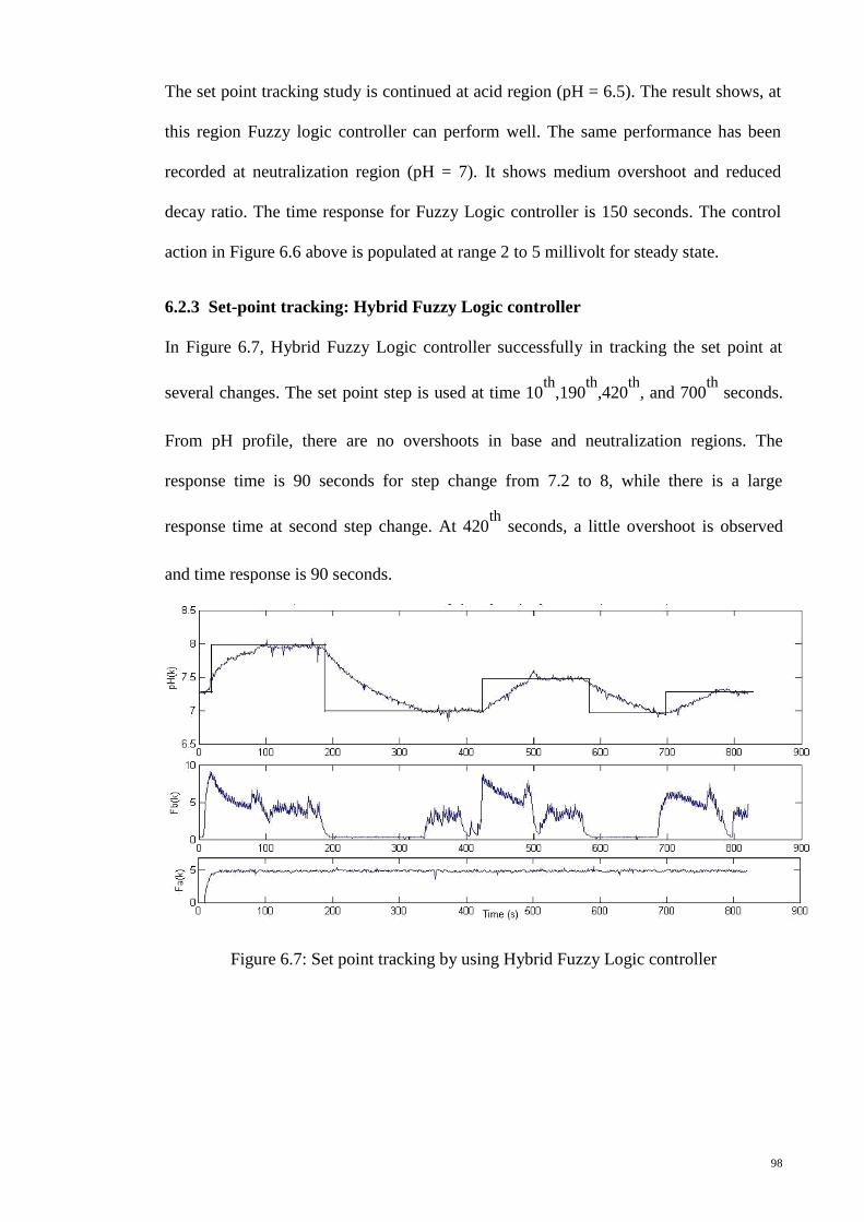
98
The set point tracking study is continued at acid region (pH = 6.5). The result shows, at
this region Fuzzy logic controller can perform well. The same performance has been
recorded at neutralization region (pH = 7). It shows medium overshoot and reduced
decay ratio. The time response for Fuzzy Logic controller is 150 seconds. The control
action in Figure 6.6 above is populated at range 2 to 5 millivolt for steady state.
6.2.3 Set-point tracking: Hybrid Fuzzy Logic controller
In Figure 6.7, Hybrid Fuzzy Logic controller successfully in tracking the set point at
several changes. The set point step is used at time 10th
,190th
,420th
, and 700th
seconds.
From pH profile, there are no overshoots in base and neutralization regions. The
response time is 90 seconds for step change from 7.2 to 8, while there is a large
response time at second step change. At 420th
seconds, a little overshoot is observed
and time response is 90 seconds.
Figure 6.7: Set point tracking by using Hybrid Fuzzy Logic controller

99
6.2.4 Disturbance rejection: PID controller
In Figure 6.8, the disturbance occurs at time 1480 seconds following increment in step
change for acid flow rate. The increment is from 5.7 to 8.3 litre/min. This disturbance
produces a change in process-variable (pH). At this time pH value drops by 0.1. The
PID controller gives the corrective action to compensate for the disturbance by
increasing the flow rate of base from 2.8 to 4.6 litre/min.
Figure 6.8: Disturbance rejection by using PID controller
The corrective action is carried out but it fail to bring the pH at 7 until the acid flow rate
returned at initial condition (5.7 litre/min).

100
6.2.5 Disturbance rejection: Fuzzy Logic controller
In Figure 6.9, the disturbance has occurred at several time span. First, the disturbance at
time 150th
, 240th
,300th
, 360th
, and 540th
seconds. The disturbance changes are in range
of 1.5 to 6 litre/min. The process variable is maintained by Fuzzy Logic controller,
which gives immediate corrective action. There is no change in the pH profile after
disturbance is introduced.
Figure 6.9: Disturbance rejection by using Fuzzy Logic controller
In Figure 6.9, Fuzzy Logic generates more frequent control action to reject the
disturbance. It gives the flow rate not stable and keeps changing from time to time. The
control action produce flow rates in range of 1.5 to 5.8 litre/min while the flow rate of
base at 0.5 to 3.8 litre/min.

101
6.2.6 Disturbance rejection: Hybrid Fuzzy Logic controller
Figure 6.10 shows, disturbance occurred once at time 40th
second. The large step
change disturbance from 5.7 to 11 litre/min is observed. The process-variable show
decrease oscillation which lead the system to steady state.
Figure 6.10: Disturbance rejection by using Hybrid Fuzzy Logic controller
In Figure 6.10, the flow rate of base is in range 4.7 litre/min. The large response time is
detected for Hybrid Fuzzy Logic controller to reject the disturbance affect.

102
6.2.7 Set-point tracking comparison
The controllability for set point tracking of controller is tested in pH neutralization
range 6.5 to 7. This range is identified as the most challenging in pH neutralization
process. As shown in Figure 6.11, all controllers succeed to reach desired set point. PID
controller has largest overshoot and fastest time response compared to others controller
followed by Fuzzy Logic and Hybrid Fuzzy Logic controller.
Figure 6.11: Set point tracking result of on-line pH neutralization
Integral Square Error (ISE) is used to find the goodness of the controllers above. The
lower the ISE number shows that controller is better compared to other controllers.
Table 6.1 shows that Hybrid Fuzzy Logic Controller has lowest ISE number which
mean it this controller produces less error at achieving the set point 7.
Table 6.1: ISE comparison for set point analysis among the controllers
Controller ISE
PID Controller 195.365
Fuzzy Logic Controller 157.652
Hybrid Fuzzy Logic Controller 35.032

103
6.3 Controller performances on Robustness issues
In Figure 6.12 below, the process-variable drops drastically after adding 1M HCl into
the reacting tank at time 1710th
seconds. The pH value drops from steady state (pH = 7)
to pH 6.3. The Hybrid Fuzzy Logic controller is able to give the corrective action to
compensate for the sudden change in the reactor.
Figure 6.12: Robustness study by using Hybrid Fuzzy Logic controller
(Altered effect in mixing reactor by adding 5ml HCL 1M)
In Figure 6.12, shows the increments of control action due to a sudden drop of reactor
concentration. It goes back to 5 millivolt which a previous steady state control action. In
Figure 6.13, the problem happens when the controlled stream became clogged. At the
first attempt, the clog start at 10% and the Hybrid Fuzzy Logic controller give
maximum control action to control valve but it fails to bring up the process-variable. It
is because the amount of NaOH entering the mixing reactor is not enough to

104
compensate for the HCl composition in the tank. The second attempt is to open at 50%
of the NaOH pipeline. At this time, the Hybrid Fuzzy Logic controller succeeds to bring
the pH value up to the desired set point with little overshoots. However, there is a delay
detected at initial corrective action at time 2465th
to 2472th seconds. It is due to the
large amount of HCL composition that populated the mixing tank due to the previous
attempt.
Figure 6.13: Robustness study by using Hybrid Fuzzy Logic controller
(Equipment failure at controlled stream)

105
Chapter 7 : Conclusion
7.1 The research novelty
The research novelties that this study proposed are:
(1) Hybrid technique of physical and empirical model
First, the proposed model of pH neutralization has been produced from first principle
and Adaptive Neural Fuzzy Inference System (ANFIS). The mechanic behind this
hybrid is in “Research Methodology” chapter. In general, this hybrid is a combination
of two output-models, which predicts the pH value. The novelty is mainly to manage the
individual output-model. The hybrid model has been validated with on-line pH
neutralization experiment and has shown a good fit (at nominal or altered conditions).
(2) The adjustment at output membership-function for Sugenno’s fuzzy inference by
introducing inverse hybrid model in Fuzzy Logic controller.
Second, this study proposed the improvement on robustness issues (in altered plant
condition) in Fuzzy Logic controller. The study improved Sugenno’s fuzzy inference
arrangement, which changed the output membership-function. The adjustment has been
made by substituting the normal output (constant or linear-function) with inverse model
prediction (model is from previous finding above). The details of the adjustment are
described in the “Research Methodology” chapter. By performing this adjustment, the
Fuzzy Logic controller is more robust when carrying out the on-line control for pH
neutralization plant. The adjusted Fuzzy Logic controller performed well compared
with conventional and Fuzzy Logic controller (with or without robustness variations).

106
7.2 Achievement of research objectives
1. The hybrid model has been obtained in this study.
The hybrid model was applied to full-scale reaction of strong acid and strong base in a
pH neutralization plant. Parallel type was the selected hybrid model structure. Online
performance analysis was conducted and compared. A mathematical model pH system
was compared with an ANFIS model pH system. A hybrid model was investigated
through several hybrid weight values α. ANFIS model alone is an insufficient
representation of pH dynamics if plant parameters is altered. Mathematical model alone
cannot best predict real pH value. The hybrid model, which combines the advantages of
the two models and meets the study objectives, is proposed. With dynamic weight
algorithm, it gives the best fit and can be used effectively in online/offline studies of
dynamic behaviour of plant pH neutralization system.
2. The Fuzzy Logic controller has been improved by inverse hybrid model.
A novel Hybrid Fuzzy Logic controller is proposed as the best advanced controller for a
nonlinear pH neutralization process control system. It is a blending between empirical
method and mathematical algorithm and this mechanism improved Sugeno type Fuzzy
Logic for robustness problem. The results have shown that it is more superior to the
other controllers (PID and Fuzzy Logic controller) in handling set point tracking and
disturbance rejection. The proposed controller has promising potential for other
nonlinear control system applications like polymerization, fermentation and many more.

107
7.3 Future work
The study can be extended for
1. Model and controller stability analysis
2. Apply proposed hybrid model and fuzzy logic controller to other nonlinear
processes
3. Improve the pilot plant design and instrument so that more advanced controllers
could be investigated
4. Implement the control system for real applications, for example, use real
wastewater instead of using standard acid and base.
5. Software interface since the control system is depended solely on
MATLAB/Simulink.

108
Reference
Akesson, B. M., Toivonen, H. T., Waller, J. B., & Nystrom, R. H. (2005). Neural
network approximation of a nonlinear model predictive controller applied to a
pH neutralization process. Computers & Chemical Engineering, 29(2), 323-335.
Altinten, A. (2007). Generalized predictive control applied to a pH neutralization
process. Computers & Chemical Engineering, 31(10), 1199-1204.
André Jones, Arnold Kaufmann, & Zimmermann, H.-J. (1986). Fuzzy Sets Theory and
Applications: Springer.
Boling, J. M., Seborg, D. E., & Hespanha, J. P. (2007). Multi-model adaptive control of
a simulated pH neutralization process. Control Engineering Practice, 15(6),
663-672.
Chaudhuri, U. R. (2001). Inferential model for pH control. Journal of Scientific &
Industrial Research, 60(7), 586-590.
Chu, J., Su, H., Gao, F., & Wu, J. (1998). Process control: Art or practice. Annual
Reviews in Control, 22, 59-72.
Coughanowr, & LeBlanc. (2008 ). Process Systems Analysis and Control.
Emami, M. R., Goldenberg, A. A., & Türksen, I. B. (2000). Fuzzy-logic control of
dynamic systems: from modeling to design. Engineering Applications of
Artificial Intelligence, 13(1), 47-69.
Figueroa, J. L., Cousseau, J. E., Werner, S., & Laakso, T. (2007). Adaptive control of a
Wiener type system: application of a pH Neutralization reactor. International
Journal of Control, 80(2), 231-240.
Filev, D. P., & Yager, R. R. (1994). On the analysis of fuzzy logic controllers. Fuzzy
Sets and Systems, 68(1), 39-66.
Galan, O., Romagnoli, J. A., & Palazoglu, A. (2000). Robust H-infinity control of
nonlinear plants based on multi-linear models: an application to a bench-scale
pH neutralization reactor. Chemical Engineering Science, 55(20), 4435-4450.
Gomez, J. C., Jutan, A., & Baeyens, E. (2004). Wiener model identification and
predictive control of a pH neutralisation process. Iee Proceedings-Control
Theory and Applications, 151(3), 329-338.
Goodwin, G. C., Mcinnis, B., & Long, R. S. (1982). Adaptive-Control Algorithms for
Wastewater-Treatment and Ph Neutralization. Optimal Control Applications &
Methods, 3(4), 443-459.
Graebe, S. F., Seron, M. M., & Goodwin, G. C. (1996). Nonlinear tracking and input
disturbance rejection with application to pH control. Journal of Process Control,
6(2-3), 195-202.
Gürocak, H. B., & de Sam Lazaro, A. (1994). A fine tuning method for fuzzy logic rule
bases. Fuzzy Sets and Systems, 67(2), 147-161.
Gustafsson, T. K. (1984). Adaptive Methods for Linear and Nonlinear Control of Ph.
Abstracts of Papers of the American Chemical Society, 187(Apr), 90-Inde.
Gustafsson, T. K., Skrifvars, B. O., Sandstrom, K. V., & Waller, K. V. (1995).
Modeling of Ph for Control. Industrial & Engineering Chemistry Research,
34(3), 820-827.
Gustafsson, T. K., & Waller, K. V. (1983). Dynamic Modeling and Reaction Invariant
Control of Ph. Chemical Engineering Science, 38(3), 389-398.

109
Henson, M. A., & Seborg, D. E. (1994). Adaptive nonlinear control of a pH
neutralization process. Control Systems Technology, IEEE Transactions on,
2(3), 169-182.
Hopgood, A. A., Goodyear, A., Nolle, L., Picton, P. D., & Braithwaite, N. S. (2002).
Automated control of an actively compensated Langmuir probe system using
simulated annealing. Knowledge-Based Systems, 15(5-6), 349-354.
Hussain, M. A. (1999). Review of the applications of neural networks in chemical
process control - simulation and online implementation. Artificial Intelligence in
Engineering, 13(1), 55-68.
Hussain, M. A., & Kershenbaum, L. S. (1999). Simulation and experimental
implementation of a neural-network-based internal-model control strategy on a
reactor system. Chemical Engineering Communications, 172, 151-169.
Ishak, A. A., M.A.Hussain, & E.Elkanzi. (2001). Modeling and control studies of
wastewater neutralization process. Paper presented at the Brunei International
Conference on Engineering & Technology, Bandar Seri Begawan.
Jang, J. S. R. (1993). Anfis - Adaptive-Network-Based Fuzzy Inference System. Ieee
Transactions on Systems Man and Cybernetics, 23(3), 665-685.
Kalafatis, A., Arifin, N., Wang, L., & Cluett, W. R. (1995). A new approach to the
identification of pH processes based on the Wiener model. Chemical
Engineering Science, 50(23), 3693-3701. doi: 10.1016/0009-2509(95)00214-p
King, P. J., & Mamdani, E. H. (1977). The application of fuzzy control systems to
industrial processes. Automatica, 13(3), 235-242.
Kuttisupakorn, P., Hussain, M. A., & Petcherdask, J. (2001). Studies on the use of
neural networks in nonlinear control strategies. Journal of Chemical
Engineering of Japan, 34(4), 453-465.
Lee, T. C., Yang, D. R., Lee, K. S., & Yoon, T. W. (2001). Indirect adaptive
backstepping control of a pH neutralization process based on recursive
prediction error method for combined state and parameter estimation. Industrial
& Engineering Chemistry Research, 40(19), 4102-4110.
Lennart, L. (2010). Perspectives on system identification. Annual Reviews in Control,
34(1), 1-12. doi: 10.1016/j.arcontrol.2009.12.001
Lu, C. H., & Tsai, C. C. (2007). Generalized predictive control using recurrent fuzzy
neural networks for industrial processes. Journal of Process Control, 17(1), 83-
92. doi: 10.1016/j.jprocont.2006.08.003
Maeda, M., & Murakami, S. (1988). A Design for a Fuzzy-Logic Controller.
Information Sciences, 45(2), 315-330.
McAvoy. (1972). Dynamics of pH in controlled stirred tank reactor. Ind. Engng Chem.
Process. Des. Develop, 11(1972), 68-70.
McCulloch, W. S., & Pitts, W. H. (1943). A Logical Calculus of the Ideas Immanent in
Nervous Activity. Bulletin of Mathematical Biophysics, 7, , 115-133.
McMillan, G. K., & Cameron, R. A. (2005). Advanced pH Measurement and Control
(3rd Edition): ISA.
Meech, J. A., & Jordon, L. A. (1993). Development of a self-tuning fuzzy logic
controller. Minerals Engineering, 6(2), 119-131.
Min, H., Bing, H., & Wei, G. (2006). Process control of pH neutralization based on
adaptive algorithm of universal learning network. Journal of Process Control,
16(1), 1-7.
Mwembeshi, M. M., Kent, C. A., & Salhi, S. (2001). An approach to robust and flexible
modelling and control of pH in reactors. Chemical Engineering Research &
Design, 79(A3), 323-334.

110
Mwembeshi, M. M., Kent, C. A., & Salhi, S. (2004). Flexible on-line modeling and
control of pH in waste neutralization reactors. Chemical Engineering &
Technology, 27(2), 130-138.
Narayanan, N. R. L., Krishnaswamy, P. R., & Rangaiah, G. P. (1997). An adaptive
internal model control strategy for pH neutralization. Chemical Engineering
Science, 52(18), 3067-3074.
Nie, J. H., Loh, A. P., & Hang, C. C. (1996). Modeling pH neutralization processes
using fuzzy-neural approaches. Fuzzy Sets and Systems, 78(1), 5-22.
Nrgaard, M., Ravn, O. E., Poulsen, N. K., & Hansen, L. K. (2000). Neural Networks for
Modelling and Control of Dynamic Systems: A Practitioner's Handbook:
Springer-Verlag New York, Inc.
Obut, S., & Ozgen, C. (2008). Online identification and control of pH in a neutralization
system. Industrial & Engineering Chemistry Research, 47(13), 4394-4404.
Rajasekaran, S., & Pai, G. A. V. (2004). Neural Networks, Fuzzy Logic and Genetic
Algorithms: Synthesis and Applications: PHI Learning Pvt. Ltd.
Rosenblatt, F. (1962). Principles of Neurodynamics Spartan. New York.
Saji, K. S., & Sasi Kumar, M. (2010, 7-9 Oct. 2010). Fuzzy Sliding Mode Control for a
pH process. Paper presented at the Communication Control and Computing
Technologies (ICCCCT), 2010 IEEE International Conference on.
Salehi, S., Shahrokhi, M., & Nejati, A. (2009). Adaptive nonlinear control of PH
neutralization processes using fuzzy approximators. Control Engineering
Practice, 17(11), 1329-1337.
Shinskey, G. (1997). Successfully controlling pH by minimizing dynamic gain -
Guidelines for designing a controllable process. Chemical Processing, 60(6), 64-
64.
Sugeno, M., & Kang, G. (1986). Fuzzy modeling andcontrol of multilayer incinerator.
Fuzzy Sets and Systems, 18, , 329-346.
Sung, S. W., Lee, I. B., Choi, J. Y., & Lee, J. (1998). Adaptive control for pH systems.
Chemical Engineering Science, 53(10), 1941-1953.
Takagi, T., & Sugeno, M. (1985). Fuzzy identication of systems and its application to
modeling and control. IEEE Transactions on Systems, Man, and Cybernetics,
15(1), 116-132.
Tan, W. W., Lu, F., Loh, A. P., & Tan, K. C. (2005). Modeling and control of a pilot pH
plant using genetic algorithm. Engineering Applications of Artificial
Intelligence, 18(4), 485-494. doi: DOI: 10.1016/j.engappai.2004.11.006
Tanaka, K., & Wang, H. O. (2002). Fuzzy Control Systems Design and Analysis: A
Linear Matrix Inequality Approach: John Wiley \\& Sons, Inc.
Vale, M. R. B. G., Fonseca, D. G. V., Pereira, K. R. C., Maitelli, A. L., Araujo, F. M.
U., & Casillo, D. S. S. (2010, 4-7 July 2010). Model Reference Adaptive Control
with inverse compensation applied to a pH plant. Paper presented at the
Industrial Electronics (ISIE), 2010 IEEE International Symposium on.
Wang, Q. C., & Zhang, J. Z. (2011). Wiener model identification and nonlinear model
predictive control of a pH neutralization process based on Laguerre filters and
least squares support vector machines. Journal of Zhejiang University-Science
C-Computers & Electronics, 12(1), 25-35.
Wright et al., R. A. W., M. Soroush and C. Kravaris. (1991). Strong acid equivalent
control of pH process. Ind. Engng Chem. Res, 30(1991), 2437-2443.
Wright, R. A., & Kravaris, C. (1995, 21-23 Jun 1995). On-line identification and
nonlinear control of an industrial pH process. Paper presented at the American
Control Conference, 1995. Proceedings of the.
Yi, S. Y., & Chung, M. J. (1995). Systematic design and stability analysis of a fuzzy
logic controller. Fuzzy Sets and Systems, 72(3), 271-298.

111
Zadeh. (1965). Fuzzy sets. Information and control, 8(3), 338-353.
Zadeh. (1994). The Role of Fuzzy-Logic in Modeling, Identification and Control.
Modeling Identification and Control, 15(3), 191-203.
Zadeh. (1996). The roles of fuzzy logic and soft computing in the conception, design
and deployment of intelligent systems. Bt Technology Journal, 14(4), 32-36.

112
Appendix A: Programming Code
File Name: ANFISMethod.m %% ANFIS method for pH model identification
%% Load traning
Dataset run
'PrepTrnDataset' trn_data = trndata(:,:); %from load
'PrepChkDataSet.m' chk_data = trn_data;
%% Select proper inputs to the model run 'InputSelection' %% Generate training ANFIS
Matrix %to prediction pH ss = 0.01;
ss_dec_rate =
0.5;
ss_inc_rate =
1.5; %Final dataset for training data trn_data = trndata(:, [input_index,
size(trndata,2)]); chk_data = trndata(:,
[input_index, size(trndata,2)]); % generate FIS matrix
in_fismat =
genfis1(trn_data); [trn_out_fismat trn_error step_size chk_out_fismat chk_error] =
...
anfis(trn_data, in_fismat, [1 nan ss ss_dec_rate
ss_inc_rate], ...
nan, chk_data, 1); %% Show result outTrn_pH = evalfis(trndata(:,input_index),
trn_out_fismat); index = 1:length(outTrn_pH); plot(index, trndata(:, size(trndata,2)), '-', index,
outTrn_pH, '.'); rmse = norm(outTrn_pH(index)-
trndata(index,size(trndata,2)))/... sqrt(length(index));
title(['Training Data (Solid Line) & ANFIS Prediction (Dots)
with RMSE = '...
num2str(rmse)]);
xlabel('Time Index');

113
ylabel(''); File Name: PrepTrnDataSet.m
%% ANFIS method for pH model
identification %PART I:
TrnDataset
%% load TrnDataSet
%% Check Time delay trndata_n = length(TrnDataSet);
subplot(3,1,1);plot(TrnDataSet(1:trndata_n
,1))
subplot(3,1,2);plot(TrnDataSet(1:trndata_n
,2))
subplot(3,1,3);plot(TrnDataSet(1:trndata_n
,3)) %% %1 output : pH pH =
TrnDataSet(:,3);
output = pH; %10 inputs : Fa(k-a),Fa(k-b),Fa(k-c),Fa(k-d),Fa(k-
e), & % Fb(k-m),Fa(k-n),Fa(k-p),Fa(k-q),Fa(k-r) input1 = [0; ...
TrnDataSet(1:trndata_n-1,1)]; input2 = [0; 0; 0; 0; 0; 0; 0; 0; 0; 0;...
0; 0; 0; 0; 0; 0; 0; 0; 0; 0;... 0; 0; 0; 0; 0; 0; 0; 0; 0; 0;... 0; 0; 0; 0; 0; 0; 0; 0; 0; 0;... TrnDataSet(1:trndata_n-40,1)];
input3 = [0; 0; 0; 0; 0; 0; 0; 0; 0; 0;... 0; 0; 0; 0; 0; 0; 0; 0; 0; 0;... 0; 0; 0; 0; 0; 0; 0; 0; 0; 0;... 0; 0; 0; 0; 0; 0; 0; 0; 0; 0;... 0; 0; 0; 0; 0; 0; 0; 0; 0; 0;... TrnDataSet(1:trndata_n-50,1)];
input4 = [0; 0; 0; 0; 0; 0; 0; 0; 0; 0;... 0; 0; 0; 0; 0; 0; 0; 0; 0; 0;... 0; 0; 0; 0; 0; 0; 0; 0; 0; 0;... 0; 0; 0; 0; 0; 0; 0; 0; 0; 0;... 0; 0; 0; 0; 0; 0; 0; 0; 0; 0;... 0; 0; 0; 0; 0; 0; 0; 0; 0; 0;... TrnDataSet(1:trndata_n-60,1)];
input5 =[0; 0; 0; 0; 0; 0; 0; 0; 0; 0;... 0; 0; 0; 0; 0; 0; 0; 0; 0; 0;... 0; 0; 0; 0; 0; 0; 0; 0; 0; 0;... 0; 0; 0; 0; 0; 0; 0; 0; 0; 0;... 0; 0; 0; 0; 0; 0; 0; 0; 0; 0;... 0; 0; 0; 0; 0; 0; 0; 0; 0; 0;... 0; 0; 0; 0; 0; 0; 0; 0; 0; 0;... TrnDataSet(1:trndata_n-70,1)];
input6 = [0; 0; 0; 0; 0; 0; 0; 0; 0; 0;... 0; 0; 0; 0; 0; 0; 0; 0; 0; 0; ... 0; 0; 0; 0; 0; 0; 0; 0; 0; 0; ... 0; 0; 0; 0; 0; 0; 0; 0; 0; 0; ... 0; 0; 0; 0; 0; 0; 0; 0; 0; 0; ...
114
0; 0; 0; 0; 0; 0; 0; 0; 0; 0; ...
TrnDataSet(1:trndata_n-60,2)]; input7 = [0; 0; 0; 0; 0; 0; 0; 0; 0; 0; ...
0; 0; 0; 0; 0; 0; 0; 0; 0; 0; ... 0; 0; 0; 0; 0; 0; 0; 0; 0; 0; ... 0; 0; 0; 0; 0; 0; 0; 0; 0; 0; ... 0; 0; 0; 0; 0; 0; 0; 0; 0; 0; ... 0; 0; 0; 0; 0; 0; 0; 0; 0; 0; ... 0; 0; 0; 0; 0; 0; 0; 0; 0; 0; ... TrnDataSet(1:trndata_n-70,2)];
input8 = [0; 0; 0; 0; 0; 0; 0; 0; 0; 0; ... 0; 0; 0; 0; 0; 0; 0; 0; 0; 0; ... 0; 0; 0; 0; 0; 0; 0; 0; 0; 0; ... 0; 0; 0; 0; 0; 0; 0; 0; 0; 0; ... 0; 0; 0; 0; 0; 0; 0; 0; 0; 0; ... 0; 0; 0; 0; 0; 0; 0; 0; 0; 0; ... 0; 0; 0; 0; 0; 0; 0; 0; 0; 0; ... 0; 0; 0; TrnDataSet(1:trndata_n-73,2)];
input9 = [0; 0; 0; 0; 0; 0; 0; 0; 0; 0; ... 0; 0; 0; 0; 0; 0; 0; 0; 0; 0; ... 0; 0; 0; 0; 0; 0; 0; 0; 0; 0; ... 0; 0; 0; 0; 0; 0; 0; 0; 0; 0; ... 0; 0; 0; 0; 0; 0; 0; 0; 0; 0; ... 0; 0; 0; 0; 0; 0; 0; 0; 0; 0; ... 0; 0; 0; 0; 0; 0; 0; 0; 0; 0; ... 0; 0; 0; 0; 0; 0; 0; 0; 0; 0; ... 0; 0; TrnDataSet(1:trndata_n-82,2)];
input10 = [0; 0; 0; 0; 0; 0; 0; 0; 0; 0;... 0; 0; 0; 0; 0; 0; 0; 0; 0; 0;... 0; 0; 0; 0; 0; 0; 0; 0; 0; 0;... 0; 0; 0; 0; 0; 0; 0; 0; 0; 0;... 0; 0; 0; 0; 0; 0; 0; 0; 0; 0;... 0; 0; 0; 0; 0; 0; 0; 0; 0; 0;... 0; 0; 0; 0; 0; 0; 0; 0; 0; 0;... 0; 0; 0; 0; 0; 0; 0; 0; 0; 0;... 0; 0; 0; 0; 0; 0; 0; 0; 0; 0;... 0; 0; 0; 0; 0; 0; 0; 0; 0; 0;... 0;0;TrnDataSet(1:trndata_n-102,2)];
input = [input1 input2 input3 input4 input5...
input6 input7 input8 input9 input10]; trndata = [input
output]; trndata(1:6,
:) = []; input_name1 = 'Fa(k-1)';
input_name2 = 'Fa(k-
40)'; input_name3 =
'Fa(k-50)'; input_name4
= 'Fa(k-60)';
input_name5 = 'Fa(k-
70)'; input_name6 =
'Fb(k-72)'; input_name7
= 'Fb(k-73)';

115
input_name8 = 'Fb(k-
74)'; input_name9 =
'Fb(k-82)'; input_name10
= 'Fb(k-102)'; File Name: InputSelection.m %% To use ANFIS we need to select the input.
% That is, to determine which variables should be the
input to the model.
% We used 10 inputs candidate; and the output is pH(k) % Input selection is selected by sequential forward
search
% to optimize the Root Mean Square Error (RMSE). %NOTE: we can use other method like Exhaustive search, GA, PSO,
and % other optimization tools
input_name = str2mat(input_name1,input_name2,input_name3,... input_name4,input_name5,input_name6,input_name7,...
input_name8,input_name9,input_name10); [input_index, elapsed_time] = seqsrch(3, trn_data,
chk_data, input_name); fprintf('\nElapsed time = %f\n',
elapsed_time); winH1 = gcf; % Group the selected input group1 = [1 2 3 4]; % y(k-a), y(k-b), y(k-c), y(k-d) group2 = [1 2 3 4]; % y(k-m), y(k-n), y(k-p), y(k-q)
group3 = [5 6 7 8 9 10]; % u(k-1) through y(k-6) anfis_n = 6*length(group3);
index = zeros(anfis_n, 3);
trn_error = zeros(anfis_n,
1); chk_error =
zeros(anfis_n, 1);
% ======= Training
options mf_n =
3; mf_type =
'gbellmf';%
epoch_n = 1; ss = 0.1;
ss_dec_rate =
0.5;
ss_inc_rate =
1.5;
% ====== Train ANFIS with different input variables
fprintf('\nTrain %d ANFIS models, each with 3 inputs
selected from 10 candidates...\n\n',... anfis
_n);
model =
1;

116
for i=1:length(group1), for
j=i+1:length(group2
), for
k=1:length(group3), in1 = deblank(input_name(group1(i),
:)); in2 =
deblank(input_name(group2(j), :));
in3 = deblank(input_name(group3(k),
:));
index(model, :) = [group1(i) group2(j) group3(k)];
trn_data = trndata(:, [group1(i) group2(j) group3(k)
... size(trndata,2)]);
chk_data = trndata(:, [group1(i) group2(j) group3(k)
... size(trndata,2)]);
in_fismat = genfis1(trn_data, mf_n, mf_type);
[trn_out_fismat t_err step_size chk_out_fismat c_err]
= ...
anfis(trn_data, in_fismat, ... [epoch_n nan ss ss_dec_rate ss_inc_rate],
... [0 0 0 0], chk_data,
1); trn_error(model) =
min(t_err);
chk_error(model) =
min(c_err); fprintf('ANFIS model = %d: %s %s %s', model, in1,
in2, in3);
fprintf(' --> trn=%.4f,',
trn_error(model)); fprintf(' chk=%.4f',
chk_error(model)); fprintf('\n'); model = model+1;
end end
end
% ====== Reordering according to
training error [a b] =
sort(trn_error);
b = flipud(b); % List according to decreasing trn error
trn_error = trn_error(b);
chk_error =
chk_error(b); index =
index(b, :); % ====== Display training and checking errors x =
(1:anfis_n)';
subplot(2,1,1
); plot(x, trn_error, '-', x, chk_error, '-', ...
x, trn_error, 'o', x, chk_error,

117
'*'); tmp = x(:, ones(1, 3))'; X = tmp(:); tmp = [zeros(anfis_n, 1) max(trn_error, chk_error)
nan*ones(anfis_n, 1)]'; Y = tmp(:);
hold on;
plot(X, Y,
'g'); hold
off; axis([1 anfis_n -inf
inf]); set(gca,
'xticklabel', []); % ====== Add text of input
variables for k = 1:anfis_n,
text(x(k), 0, ... [input_name(index(k,1), :) ' ' ...
input_name(index(k,2), :) ' ' ... input_name(index(k,3), :)]);
end h = findobj(gcf, 'type', 'text'); set(h, 'rot', 90, 'fontsize', 11, 'hori', 'right'); drawnow % ====== Generate
input_index [a b] =
min(trn_error);
input_index = index(b,:);
title('Training (Circles) and Checking (Asterisks)
Errors'); ylabel('RMSE');

118
Appendix B: MATLAB/Simulink
1. Pilot Plant Data Acquisition Block Diagram
2. Collecting Online Dataset
sizeFb = size(Fb.signals.values(:,:,:),3);
for i = 1:sizeFb
time(i) = i;
CVa(i) = Cv_acid.signals.values(i);
CVb(i) = Cv_base.signals.values(i);
FaData(i) = Fa.signals.values(:,:,i);
FbData(i) = Fb.signals.values(:,:,i);
pHData(i) = pH1.signals.values(:,:,i);
end
Dataset = horzcat(FaData',FbData',pHData');


