Neural Net Stock Trend Predictor - SJSU Computer Science ...The Designated Project Committee...

Neural Net Stock Trend Predictor

A Project Presented to

The Faculty of the Department of Computer Science

San Jose State University

In Partial Fulfillment of the Requirements

Of the Degree

Master of Science

By

Sonal Kabra

May 2017

!i

© 2017

Sonal Kabra

ALL RIGHTS RESERVED

!ii

The Designated Project Committee Approves the Master’s Project Titled

Neural Net Stock Trend Predictor

by

Sonal Kabra

APPROVED FOR THE DEPARTMENT OF COMPUTER SCIENCE

SAN JOSE STATE UNIVERSITY

May 2017

___________________________________________________________________

Dr. Chris Pollett, Department of Computer Science Date

___________________________________________________________________

Dr. Robert Chun, Department of Computer Science Date

___________________________________________________________________

Mr. Paul Thienprasit, Cisco Date

APPROVED FOR THE UNIVERSITY

__________________________________________________________________

Associate Dean Office of Graduate Studies and Research Date

!iii

ACKNOWLEDGEMENT

This work is devoted to my husband whose trust in my capacities and unremitting

support motivates and stimulates me each and every day of my life. I want to thank

my project advisor, Dr. Chris Pollett, for his persisting patience and steady guidance

all through this project. I also, likewise, want to extend my gratitude to the board of

committee members, Dr. Robert Chun and Mr. Paul Thienprasit, for their

recommendations and time.

!iv

Abstract

This report analyzes new and existing stock market prediction techniques. Traditional

technical analysis was combined with various machine-learning approaches such as

artificial neural networks, k-nearest neighbors, and decision trees. Experiments we

conducted show that technical analysis together with machine learning can be used

to profitably direct an investor’s trading decisions. We are measuring the profitability

of experiments by calculating the percentage weekly return for each stock entity

under study. Our algorithms and simulations are developed using Python. The

technical analysis methodology combined with machine learning algorithms show

promising results which we discuss in this report.

!v

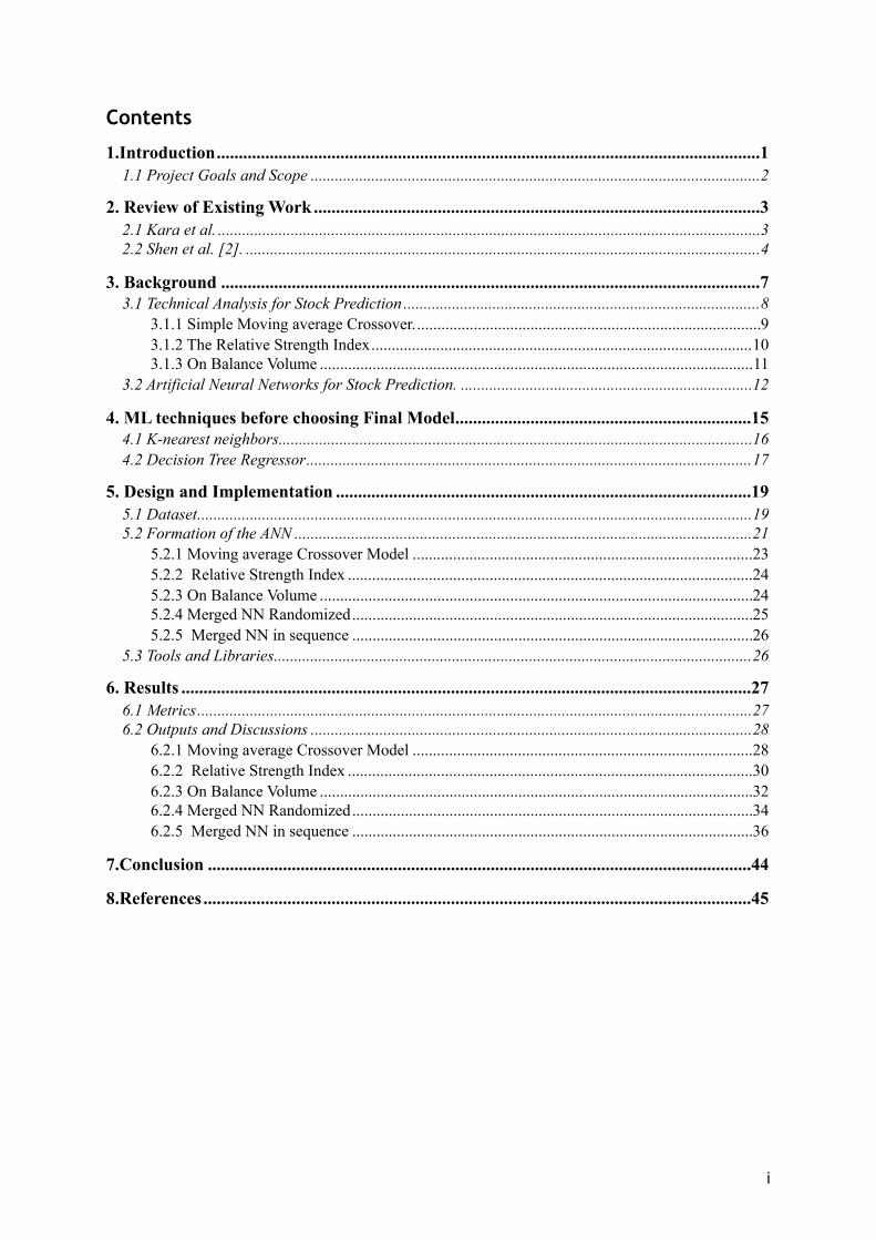
Contents

1.Introduction 1 ...........................................................................................................................1.1 Project Goals and Scope 2 ...............................................................................................................

2. Review of Existing Work 3 .....................................................................................................2.1 Kara et al. 3 ......................................................................................................................................2.2 Shen et al. [2]. 4 ...............................................................................................................................

3. Background 7 ..........................................................................................................................3.1 Technical Analysis for Stock Prediction 8 ........................................................................................ 3.1.1 Simple Moving average Crossover. 9 ..................................................................................... 3.1.2 The Relative Strength Index 10 .............................................................................................. 3.1.3 On Balance Volume 11 ...........................................................................................................3.2 Artificial Neural Networks for Stock Prediction. 12 ........................................................................

4. ML techniques before choosing Final Model 15 ...................................................................4.1 K-nearest neighbors. 16 ....................................................................................................................4.2 Decision Tree Regressor 17 ..............................................................................................................

5. Design and Implementation 19 ..............................................................................................5.1 Dataset 19 .........................................................................................................................................5.2 Formation of the ANN 21 ................................................................................................................. 5.2.1 Moving average Crossover Model 23 .................................................................................... 5.2.2 Relative Strength Index 24 .................................................................................................... 5.2.3 On Balance Volume 24 ........................................................................................................... 5.2.4 Merged NN Randomized 25 ................................................................................................... 5.2.5 Merged NN in sequence 26 ...................................................................................................5.3 Tools and Libraries 26 ......................................................................................................................

6. Results 27 .................................................................................................................................6.1 Metrics 27 .........................................................................................................................................6.2 Outputs and Discussions 28 ............................................................................................................. 6.2.1 Moving average Crossover Model 28 .................................................................................... 6.2.2 Relative Strength Index 30 .................................................................................................... 6.2.3 On Balance Volume 32 ........................................................................................................... 6.2.4 Merged NN Randomized 34 ................................................................................................... 6.2.5 Merged NN in sequence 36 ...................................................................................................

7.Conclusion 44 ...........................................................................................................................

8.References 45 ............................................................................................................................

!i

LIST OF FIGURES

1. Simple Moving Average Crossover vs. Price..................................................11

2. RSI vs. Price ..................................................................................................12

3. ANN Diagram .................................................................................................14

4. KNN Output ....................................................................................................18

5. Decision Tree output ......................................................................................19

6. Merged artificial neural network......................................................................26

7. Moving average crossover Model weekly output............................................30

8. RSI weekly output...........................................................................................32

9. OBV Model weekly output...............................................................................34

10.Merged NN Randomized Model weekly output...............................................36

11. Merged NN in Sequence Model weekly output...............................................38

!ii

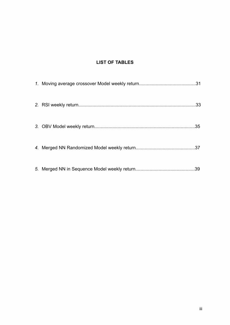
LIST OF TABLES

1. Moving average crossover Model weekly return............................................31

2. RSI weekly return...........................................................................................33

3. OBV Model weekly return..............................................................................35

4. Merged NN Randomized Model weekly return..............................................37

5. Merged NN in Sequence Model weekly return..............................................39

!iii

Chapter 1

Introduction

Since the beginning of the stock market in 1817 in the United States, its accurate

prediction has been a goal of investors. Every day millions of dollars are invested in

the stock exchange, and behind each dollar is a trader hoping to earn a profit in one

way or another. The stock market offers the promise of monetary returns if a trader

can accurately predict market trends and fluctuations. So it is not a big surprise that

the stock market makes its way into the public consciousness each time it

misbehaves, i.e., it fails to be predictable. The 2008 stock market crash was followed

by a surge of movies and documentaries. If there was a common theme among

those movies and documentaries, it was that a few individuals were able to foresee

the impending crash. Maybe a superior technique for stock market forecast would

help with comparable occasions in the future.

A stock market is the most critical aspect of any country's economy. It is one of the

most powerful ways for a nation’s companies to build capital and also a great

investment tool for investors as well as ordinary people [3][4][5]. The most crucial

problem for the prediction of stocks is its dependency on a high number of market

variables. There are multiple political, environmental, and financial factors, which can

influence stock prices on a global scale. For example, the political stability of a nation

can directly influence the stock prices in world economy. However, the impact is

limited to only those companies which are directly or indirectly related to the

!iv

concerned variable in some way. Because of all these challenges, researchers have

had to invent different techniques to predict the stock market correctly. The financial

sector is an appropriate platform for the utilization of numerous artificial intelligence

technologies. The consistency of the stock exchange has perpetually been

questioned in economic studies. Despite that, the challenge of stock anticipation is

so appealing because even an iota of improvement can increase benefit by a huge

amount of dollars for these institutions and traders.

1.1 Project Goals and Scope

To predict the market for their clients or themselves, financial institutions or individual

traders have created plenty of proprietary models, but it has been rare to achieve

even more-than-average returns on an investment consistently. Stock market

prediction is a secretive and experimental art and only a limited number of people

who have succeeded in mastering this art will share what strategies they have

designed. Stock market investments are never easy, because of the high volatility

and the dynamic nature of stock market variables.

Keeping all these variables in mind, we have designed a tool, the "Neural Net Stock

Trend Predictor", as a part of the project. The primary goal of this tool is to utilize

available academic understanding and develop an approach to predict stock market

movement and indicate whether the stock under study should be -- Bought, Neutral,

or Sold to generate profit. This tool makes predictions only for the following week.

In this report, Chapter 2 presents a review of existing work done in this field. Chapter

3 contains multiple concepts and definitions of the project. Chapter 4 includes other

machine learning techniques implemented before choosing the neural network as a

!v

model for this project. Chapter 5 describes the different design and implementation

techniques used. Chapter 6 discusses the result obtained by the implementation

discussed in Chapter 3. Chapter 7 presents the conclusion. The report ends with

references in Chapter 8.

!vi

Chapter 2

Review of Existing Work

This chapter reviews existing academic literature regarding predicting the stock

market. It will look at the technical analysis methods and the machine learning

methods used and implemented till date.

2.1 Kara et al. [1]

This article uses the Artificial Neural Network (ANN) and the Support Vector Machine

(SVM) for the prediction of direction of stock price index movement. The author used

the ISE National 100 Index for the dataset and traded on the Istanbul Stock

Exchange.

The tool has achieved up to 75.74% accuracy in this prediction model.

It uses a total of 10 technical analysis indicators:

1. Simple 10-day moving average

2. Larry Williams R%

3. Relative Strength Index

4. Momentum

5. Commodity Channel Index

6. Stochastic D%

7. Weighted 10-day moving average

8. Accumulation Distribution Oscillator

9. Moving Average Convergence Divergence

10.Stochastic K%

!vii

The values of the above technical indicators are calculated based on daily stock

prices. The author has combined these results with the daily price movement

direction. Two models experiment with this data- the first model is a neural network

with an accuracy of 75.74% and the second one is the SVM with an accuracy of

71.52%.

In our research, instead of combining all the technical indicators together for the

training of neural net, the artificial neural network will test each technical indicator.

2.2 Shen et al. [2].

This paper predicts the movement in American stock exchange and the Dow Jones

Industrial Average. It uses various financial products like FTSE index price, Oil price,

DAX index price, and the EURO/USD exchange rate for it. The author uses the

movement predicted by these financial products and the machine learning

techniques to forecast the stock market. The author claims an accuracy of 77.6% for

the Dow Jones specifically.

It compares two models - a Support Vector Machine and a Multiple Additive

Regression Tree. The tool claims an accuracy of 74.4% with the support vector

machine model.

Apart from the machine learning techniques mentioned above, plenty of other

models and theories have been put forward for consideration. Each method has its

own pros and cons. Random Walk Hypothesis theory suggests that the stock data

follows a random pattern; therefore it can never be predicted. [6].

!viii

On the other side, many individuals are convinced of the fact that market pursues a

trend and hence, can be predicted; if one studies and observes it for an extended

period of the time, the stock price can then be predicted.

Most of the researchers use historical stock data for prediction. This data usually

contains information like the opening and closing prices, highest and the lowest

prices of the day, etc. The values generated are because of the transaction of the

stock entity in the market.

A famous quote from Fama, 1965 is, “To what extent can the history of a common

stock’s price be used to make meaningful predictions concerning the future price of

the stock?” [3] This question can effectively be applied to the working of ANN.

For many years, various traditional and statistical methods have been used to predict

the stock market. The traditional methods like linear regression, time series analysis,

and chaos theory were popular [9]. But because of the unpredictability of the stock

market, these methods were only partially successful [10].

More modern soft computing techniques such as neural networks, fuzzy systems,

regression, and classification have been proposed to solve this forecasting problem

as they can capture the non-linearity of the data more efficiently. [11][12][5]

Apart from the above work, multiple types of research propose the technical analysis

indicators as one of the most efficient and effective tools in identifying a trend and

predict prices of the stock market for the near future [7][8].

With the advancement of innovation and science, numerous new scientific and

technological strategies have been suggested for stock value forecasting for, e.g.,

Genetic Algorithm, or Neural Networks, etc.[13][8].

!ix

Certain data trends such as the prediction of the stock market prices are nonlinear in

nature. To generalize and learn from such nonlinear patterns, ANN can be used as

proven from the various papers mentioned above. ANN also allows a certain degree

of deviation in the input and output values as the network automatically adjust to the

data pattern. Thus, ANN provides a better and more efficient way to generalize the

trends compared to other methods. [14]

In all of the above techniques, the basis of predictions of the stocks is either via the

models based on various algorithms or through technical analysis of data. Most of

the above techniques try to obtain the same result, which is to forecast whether

stock prices will either rise or fall.

In our research, instead of predicting Up/Down signals, it will predict stock trade

signals, namely “Buy, Sell or Neutral” for the next week.

!x

Chapter 3

Background

Any entity in the stock market will have five main data features associated with it:

1. ‘Open’: Stock entity's opening price for the day.

2. ‘High’: Stock entity's highest price for the day.

3. ‘Low’: Stock entity's lowest price for the day.

4. ‘Close’: Stock entity's closing price for the day.

5. ‘Volume’: The quantity of stocks exchanged on the day

Throughout the project, all of the features developed using technical analysis

indicators will be calculated based on the above data.

To earn profit from investing in the stocks is the most challenging task for any

investor. The investor can be any individual either from the inside or outside of the

business sector [15].

Most of the investors follow two analytical methods to select which stock to buy,

neutral or sell and when [7][15]:

1. Fundamental analysis:

This analytical method studies and reports company’s fundamental factors such as

balance sheets, profit, and loss, along with various ratios like price to earning (P/E),

price to book value (P/BV), price to earning growth, and earnings per share (EPS). It

assesses the economic health of the company and evaluates its market perspective.

These factors help to find the current value of the company and predict the future

profits thus helping the investors to find the stocks worth investing.

!xi

2. Technical analysis:

This method reports essential features of any stock entity like the opening price,

volume, etc. It does not try to identify the value of the particular stock object. This

approach uses various charts overlapping each other and essential features, and

with the help of tools, it identifies the patterns that can suggest future uptrend or

downtrend activity of the stock.

Some automatic stock trading systems take advantage of both the above-mentioned

analytical methods while other focus on only one method.

3.1 Technical Analysis for Stock Prediction

Technical Analysis is simple, instinctive and a very easy to learn technique for any

individual. It uses multiple charts plotted on the top of each other. By analyzing them,

one can grasp the subsequent market movement. This method is very effective for

short-term trading. Since this analysis utilizes the historical information of the stock, it

can easily generate signals for short-term fluctuations by using the recurring patterns

and trends within the stock data features for the predictions.

As in our research, the stock signals generated are for the next week. Therefore, we

will consider technical analysis for stock prediction instead of fundamental analysis.

By observing the money flow, momentum, and volatility, technical analysis

supplements in confirmation of trends or patterns of the stock.

Technical analysis indicators are of two types: the leading and lagging indicator. The

leading indicator precedes the stock price movement, while the lagging indicator

follows the stock price movement. The leading indicator generates the signal before

any new trend or reversal may occur. The lagging indicators will generate the signal

later. [7]

!xii

For current research, we are going to consider both types of technical indicators.

The basic idea is to acquire the stock price historical data of S&P 500 index

companies. Later on, we pre-process the data and build the features based on the

input data. The features are three technical indicators: Simple moving average for 5-

Day and 10-Day, Relative Strength Index and On Balance Volume.

3.1.1. Simple Moving Averages(SMA) Crossover

The most common lagging indicator technique is a simple moving average. An N-

period SMA calculated is the mean of the preceding N periods' price. [7]

! [7]

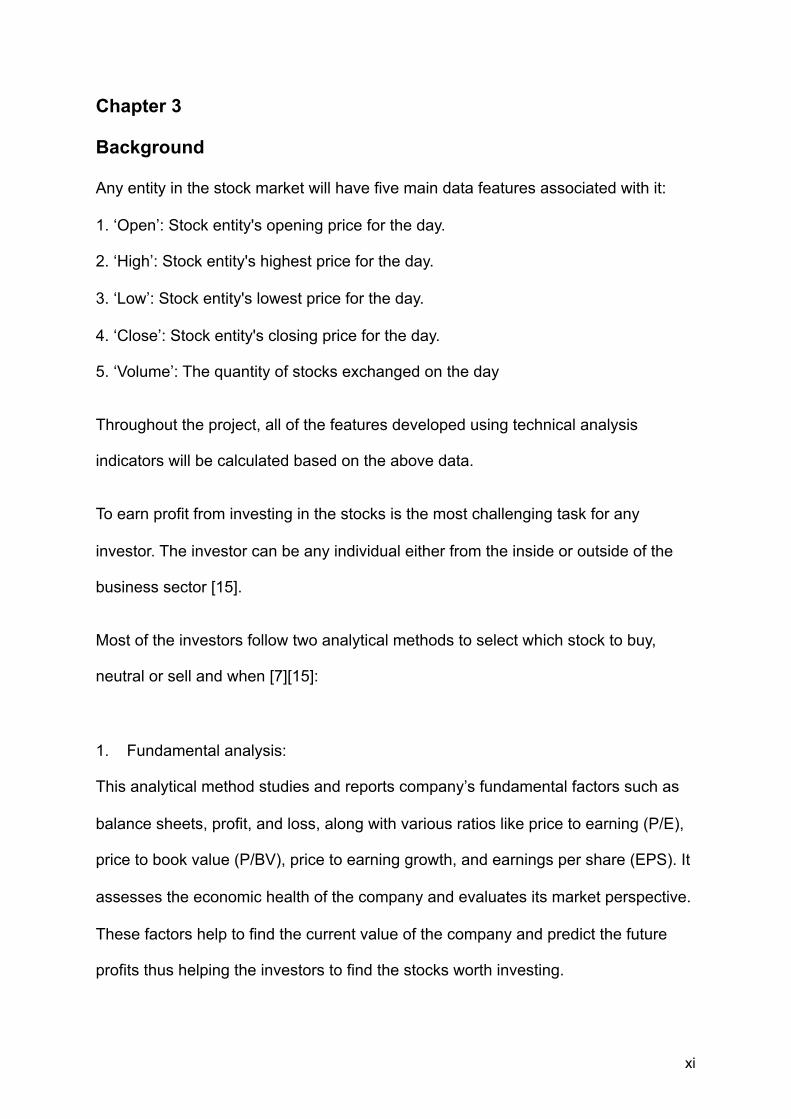
In this research, 5-days SMA and 10-day SMA crossover strategies are used for the

stock prediction. When a short period (5-days) SMA crosses over a long period (10-

day) SMA, then it signals to buy. Similarly, when a short period (5-days) SMA falls

below a long period (10-day) SMA, then it signals to sell. The demonstration of this

strategy can be seen in the following figure.

From the figure 1, it shows that the moving average crossover follows the trend in

price movement.

!xiii

!

Fig1. Simple Moving Average Crossover vs. Price

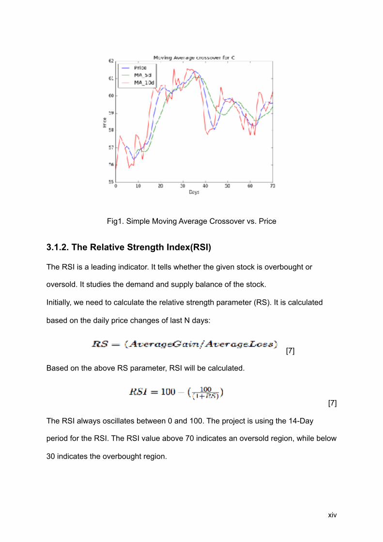
3.1.2. The Relative Strength Index(RSI)

The RSI is a leading indicator. It tells whether the given stock is overbought or

oversold. It studies the demand and supply balance of the stock.

Initially, we need to calculate the relative strength parameter (RS). It is calculated

based on the daily price changes of last N days:

! [7]

Based on the above RS parameter, RSI will be calculated.

! [7]

The RSI always oscillates between 0 and 100. The project is using the 14-Day

period for the RSI. The RSI value above 70 indicates an oversold region, while below

30 indicates the overbought region.

!xiv

Whenever the stock reaches in the overbought region, it crosses the line down. Thus

generating the downtrend and then the sell signal is triggered. Similarly, if the stock

is in the oversold region, it crosses the oversold line up and triggers buy signal.

The following figure explains this phenomenon:

!

Fig 2. RSI vs. Price

3.1.3. On-Balance Volume (OBV)

OBV is a volume-based momentum indicator. Volume is the most important stock

data feature. It focuses on how it can affect stock's price and its momentum. It is

used to find the buying and selling trend of the stock. It calculates the positive and

negative flow of the volume on its price.

The value for OBV can be calculated as follows.

!xv

If the current closing price is more than the previous close price:

!

If the current closing price falls below the previous close price:

!

Else it will just assign the previous OBV to current OBV.

This indicator demonstrates that the volume precedes the price of the stock. For,

e.g., if the OBV is following the same trend as that of the price in the same direction

then the trend of the stock will be same. If the OBV moves against the price trend,

then it signals that the current trend is weakening and might reverse.

3.2 Artificial Neural Networks for Stock Prediction

ANNs are the computational models utilizing programming systems to replicate the

behavior and adapt the features of biological neural systems. [18]

ANN has tens, hundreds or thousands of artificial neurons just like a human brain

has neuron nodes. The artificial neuron has an input unit, which receive inputs from

the environment. This neuron will be fired on the specific condition, and it will

transmit the signal to the connected neurons. Figure 3 represents an artificial

neuron.

A numerical positive and negative relates to every neuron to either restrain or

energize the input with each connection to the artificial neuron. An activation function

controls the termination of an artificial neuron. The artificial neuron gathers the

approaching signals by processing its input signal as an operator with associated

!xvi

weights. These input signals now serve as input to the activation function, which

computes the output signal of artificial neurons. [19]

Fig. 3: ANN [19]

ANN stands out amongst the most well known classification algorithms, as it caters a

high-efficiency prescient model within complex information. There are three essential

layers in the ANN model. [15]

1. Input Layer: This layer comprises of nodes or all input features in the training

set. These nodes impart all the input data into hidden layers.

2. Hidden Layer: This layer comprises of a node responsible for processing and

learning of data from the input layer, alluded as perceptron.

3. Output Layer: This layer comprises of a class node, computed mostly by

sigmoid function or any other activation function. Outer layer sends

information straight to a PC gadget or a mechanical control system.

ANN consolidates two working stages - the first stage is the period of learning and

the second phase is the period of recall. The known historical data sets train the

signal in both input and output layers in the learning stage. The weight acquired is

utilized in the recall stage.

!xvii

Using neural systems to model and forecast the course of stock market returns has

been the subject of recent factual and theoretical examinations by scholastics and

professionals. [16] ANNs can perceive and learn related patterns amongst input

values and respective real target values. As the nature of the stock market is

complex and volatile, ANNs can be chosen to unravel the mystery of the stock

market as they have the ability to deduce the result from unpredicted data, mostly for

dynamic systems that change in real time.

!xviii

Chapter 4

ML techniques before final model

Whenever any human invests in stocks, he/she tries to study the past data to find the

similar pattern. This project uses K-nearest neighbor and the Decision tree machine

learning regression techniques to follow the same trend by predicting just using

historical data. Both of these techniques are useful in capturing past data and

predicting based on that.

By using those techniques, we are predicting the closing price of the same day.

The input data for both methods are past year data. The main features are open,

high, low and volume.

To enhance the predicting capabilities for these AI techniques, we used the Bagging

Regressor ensemble method. Ensemble methods are the type of learning algorithm

that learn by creating classifiers or multiple models based on past data and then

classifying new data either by voting, bagging or boosting. Preliminary work uses the

Bagging Ensemble method and it will help us to create multiple models from the

original dataset.

The best parameters for both ML techniques are computed using grid search

algorithm. It tunes the hyper-parameters by using cross-validation. Cross-validation

is a technique for creating validation datasets from the given training data set. Once

the model trains on the remaining dataset, the validation datasets then test the

model. Thus, this helps to avoid the overfitting problem.

!xix

4.1 K-nearest neighbor

KNN algorithm defines a correlation between prediction values and objects. There is

a prediction value associated with each object. The algorithm states that the

prediction values are similar for the objects that are in close proximity of each other.

Thus, we can assume that the prediction values will be almost equal for such

objects. [20]

The KNN is an instance-based learning algorithm. It calculates the closest distance

of the data points, and uses this value to figure out the category of the new vector in

the training data set. During the training phase of the algorithm, the entire feature

space gets divided into different regions. For each input data point, the distance from

the input data is calculated. This distance is then used to categorize the point to a

particular category. The data points with similar contents map to the same region in

the feature space. [21]

The output after running the stock prediction using KNN for CISCO, and Facebook is

as shown in the following figure:

It is evident from the figure that KNN has a high error range for both stocks with

tuned parameters and the predictions are completely off from the right prices. Thus,

a k-nearest neighbor is not a very potent stock price predictor.

!xx

!

Fig. 4 K-NN output

4.2 Decision Tree Regressor

Decision trees divide the information into small gatherings based on maximizing

information gain. In this way, these gatherings catch the historical stock data and

anticipate information that is similar to this data.

The decision trees learn the details of the training set based on the height of the tree

set. Thus, if the maximum height of the tree is set to a large value, then there is the

risk of considering the noise along with the training data. This pattern is called

overfitting.

The aim of this process is to generate a model that will help figure out the final value

based on the rules deduced from the data features.

The output after running the stock prediction using Decision Tree regressor for the

Google stock is as shown in the following figure:

!xxi

!

Fig. 5 Decision Tree Output

The actual close value for GOOG is 750.50, while it’s predicted value is 745.21. The

error range is reduced with decision tree, but the predicted value is still not effective.

!xxii

Chapter 5

Design and implementation

The design and implementation process of Artificial Neural Networks consists of four

steps. These steps explain the implementation process and how ANNs are divided

into the different stages of the design.

The initial step is to choose the data that will be used in neural networks. This

information would be used for processing during the various phases of ANN.

The second step is to tweak the quantity of hidden nodes utilized inside ANN.

The third step involves optimizing the time window that used in the input phase.

The final step involves making an informed decision by selecting the best network

out of all the networks tested.

5.1 Dataset

For this project, the S&P 500 market is selected as a representative of the stock

market. S&P 500 is an index of 500 large-cap American stocks. S&P 500 companies

are widely known & are pioneers in their sectors. This market blankets a diverse set

of multinational corporations such as Apple, Citigroup, and MacDonald thus

commonly used as a representation of the entire US stock market

Collecting the Datasets

Various websites have the functional capabilities to provide daily historical stock

data. Some companies like Google and Yahoo have financial websites that allow the

!xxiii

user to gain access and download excel sheets, which contain the previous stock

data for a company which is a useful feature and very helpful when the user wants to

gather information about a particular company. However, such websites are not

useful when the user wants to access stock data of multiple companies, which can

lead to large data gathering.

To solve this issue, Quandl is used. Quandl is available at no cost for users to use. It

provides an excellent alternate to Google and Yahoo websites. Quandl hosts large

amounts of datasets, which is focused specifically on the stock market data. Google

and Yahoo back this data up. However, Quandl maintains it.

Quandl also enables the users to access this database with the help of a small

python library that it provides.

The python Quandl API allows users to query historical stock prices from databases.

Thus can be asked each time while running the program to gather the stocks of

companies in the S&P 500. This project trains ANN model on 1000 days of inventory

data.

Data Preprocessing

All the features (technical indicators and stock details) in the data set are not in

similar range. Features such as the volume of the stocks apply more impact to

prediction compared to smaller values in the data set, like the stock price. Hence, it

is advised to consider all the features in the dataset at the same scale.

Normalizing data sets can minimize the fluctuation and noise associated with the

data.

!xxiv

The values in datasets are normalized in the range of [-1,1]. For that

Sklearn.MinMaxScaler() library function is used. Sklearn is a simple and efficient tool

for data mining and data analysis.

The transformation is:

!

Here, min is -1 and max is 1.

5.2 Formation of the ANN

The ANN used in this project comprised of one input layer, two hidden layers, and

one output layer. To improve the accuracy of the prediction and catch more patterns,

multiple hidden layers can be chosen. Therefore, two hidden layers are preferred.

Input Layer

The product of the number of features in the dataset series and the window size

gives the number of neurons used in the layer of entry. The window size is the

duration in days.

The input signals in the layer of entry are technical indicators and the closing price of

stock. The number of these input signals changes from twenty to thirty contingent

upon the number of technical indicators picked.

!xxv

Hidden Layer

The total neurons in the hidden layer are obtained through experimental results. The

broad spectrum from n/2 to 4n formula is used, where n is some neurons in the input

layer. The number of 2n neurons is somewhat more efficient for this problem. The

activation function chosen for this layer was tanh.

Output Layer

The number of the prediction classes defines the output layer neurons. The chosen

activation function is sigmoid.

Training Algorithm

The back propagation algorithm can be used to adjust the weight values in the

reverse direction. This algorithm makes use of a computed output error to (or

“intending to”) adjust weights. To figure out the value of output error, a forward

propagation phase needs to be completed before the process is started. During the

process of forward propagation, the activation function is used. This enables the

activation of the neurons. The RProp (Resilient Propagation) algorithm was chosen

because several works from the literature indicate that it performs better than the

standard back propagation in different contexts.

However, the two principal issues can arise in the network system: overfitting and

underfitting. In case, the network fails to generalize the data and tries to memorize

the training data, it leads to the issue of overfitting. When the system fails to follow

the data provided, the network goes into a state of underfitting.

!xxvi

The data is partitioned into the training (70% of the dataset), the validation (20%)

data set, and test (10%) data set to avoid overfitting and uderfitting.

ANN uses the training data set that is provided to find a generic pattern between

input and output values. The validation data set provided to the network enables it to

figure out if the training data follows the correct pattern. The test data set makes sure

that the prediction quality that is produced by ANN follows the norm as per the

training set.

Testing Dataset

The 100 data points are randomly held from the generated dataset. The neural net is

trained on around 800 stock data points, and later tested on 100.

Following are neural network architectures developed during this project:

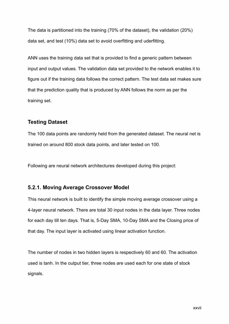
5.2.1. Moving Average Crossover Model

This neural network is built to identify the simple moving average crossover using a

4-layer neural network. There are total 30 input nodes in the data layer. Three nodes

for each day till ten days. That is, 5-Day SMA, 10-Day SMA and the Closing price of

that day. The input layer is activated using linear activation function.

The number of nodes in two hidden layers is respectively 60 and 60. The activation

used is tanh. In the output tier, three nodes are used each for one state of stock

signals.

!xxvii

5.2.2 RSI Model

This neural network is built to identify the demand and supply effect using the

relative strength index using the 4-layer neural network. There are total 20 input

nodes in the data layer. Two nodes for each day till ten days, which is a 14-Day RSI

and Closing price of that day. The data layer is activated using linear activation

function.


used is tanh. In the output level, three nodes are used each for one state of stock

signals.

5.2.3 OBV Model

This neural network is built to identify the buying and selling trend using On Balance

Volume index using the 4-layer neural network. There are total 30 input nodes in the

data layer. Three nodes for each day till ten days. The nodes are on balance volume

of the day, Volume of the day and Closing price of that day. The input layer is

activated using linear activation function.


used is tanh. In the output tier, three nodes are used each for one state of stock

signals.

5.2.4 Merged NN Randomized

For this experiment, modules mentioned above are merged into the final layer of the

neural network as shown in the following figure. The whole architecture is trained

!xxviii

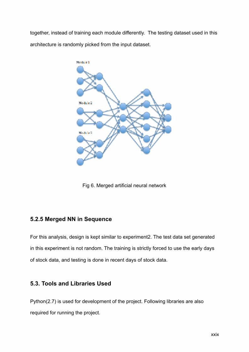
together, instead of training each module differently. The testing dataset used in this

architecture is randomly picked from the input dataset.

!

Fig 6. Merged artificial neural network

5.2.5 Merged NN in Sequence

For this analysis, design is kept similar to experiment2. The test data set generated

in this experiment is not random. The training is strictly forced to use the early days

of stock data, and testing is done in recent days of stock data.

5.3. Tools and Libraries Used

Python(2.7) is used for development of the project. Following libraries are also

required for running the project.

!xxix

● Keras (Neural Network Library)

● Sklearn (Machine learning and data analysis library)

● Numpy (for mathematical calculations)

● Matplotlib (Plotting the results)

● Quandl API (Stock data)

● Pandas (storing stock data structure)

!xxx

Chapter 6

Results

6.1 Metrics

As this is a multi-classification problem ("Buy," "Sell," or "Neutral"), the accuracy

metric used is a confusion matrix. Accuracy defined is the number of correctly

classified points in comparison to the total number classifications made. The neural

net model implemented in the course of this project experiments on following stocks

to collect results: Apple (AAPL), Citi Groups (C), Caterpillar (CAT), Exxon Electronics

(XOM), Home Depot (HD), McDonald's (MCD).

Evaluation Measurement

Accuracy will be calculated as:

!

Where,

True_Buy = all the true positives values of buy

True_Sell = all the true positive values of sell

True_neutral = all the true positives values of neutral

!xxxi

Based on the above formula, accuracy & standard deviation is computed for each

experiment & displayed in following format [accuracy% [standard deviation%]]. As

the research is generating buy, hold and sell signals, the false classified hold signal

will not affect the stock investor adversely. Hence we will consider the ratio of true

positive (buy and sell) and false negative (buy and sell). The ratio is written below

the confusion matrix for each stock.

Normalized percentage weekly return

To find out the profitability of the proposed models, normalized percentage weekly

return is calculated using the following formula:

!

6.2 Outputs and Discussions

6.2.1 Moving average crossover Model

! !

!xxxii

AAPL [Acc.42.60%(5.16%)] 1.23

CAT [Acc.40.90%(6.16%)] 1.42

! !

! !

Fig. 7: Moving average crossover Model Output

Discussion:

After observing the ratio of the true positive (buy and sell) and the false negative

(buy and sell) of stock's confusion matrix for the above model, the model is doing

relatively good for all the stocks, as the ratio is above 1 for all of them. The

normalized percentage weekly return values are given in TABLE 1.

!xxxiii

C [Acc. 47.00%(4.16%)] 2.72

MCD [Acc. 36.40%(7%)] 1.31

XOM [Acc.34.80%(3.76%)] 3.71

AAPL [Acc.42.60%(5.16%)] 1.23

Table 1: Moving average crossover Model weekly return

From the above table, the standard risk-free rate of weekly return is 0.035%. For

this model, all but the HD is giving good return, though with some risk. Thus, this

model is doing relatively good.

6.2.2 RSI model

! !

Stocks Percentage weekly return

AAPL 0.066%

MCD 0.088%

XOM 0.076%

CAT 0.104%

C 0.1%

HD 0.012%

!xxxiv

AAPL [Acc. 47.80%(6.14%)] 1.34

CAT [Acc.37.40%(6.41%)] 1.87

! !

! !

Fig. 8: RSI Model

Output

Discussion:



relatively good for only 4 of the total stocks. The normalized percentage weekly

return values are given in TABLE 2.

!xxxv

HD [Acc.37.40%(9.71%)] 1.30

C [Acc.47.00% (9.8%)] 2.13

MCD [Acc.36%(1.67%)] 1.32

XOM [Acc.29.60%(8.16%)] 0.71

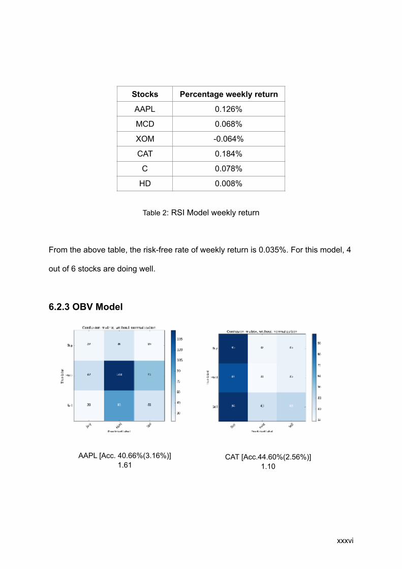
Table 2: RSI Model weekly return

From the above table, the risk-free rate of weekly return is 0.035%. For this model, 4

out of 6 stocks are doing well.

6.2.3 OBV Model

! !


AAPL 0.126%

MCD 0.068%

XOM -0.064%

CAT 0.184%

C 0.078%

HD 0.008%

!xxxvi

AAPL [Acc. 40.66%(3.16%)] 1.61

CAT [Acc.44.60%(2.56%)] 1.10

! !

! !

Fig. 9: OBV Model Output

Discussion:





!xxxvii

HD [Acc. 34.20%(1.16%)] 0.77

C [Acc. 46.80%(4.58%)] 1.16

MCD [Acc.30.40%(5.16%)] 0.98 XOM [Acc. 33.60%(5.60%)]

0.97

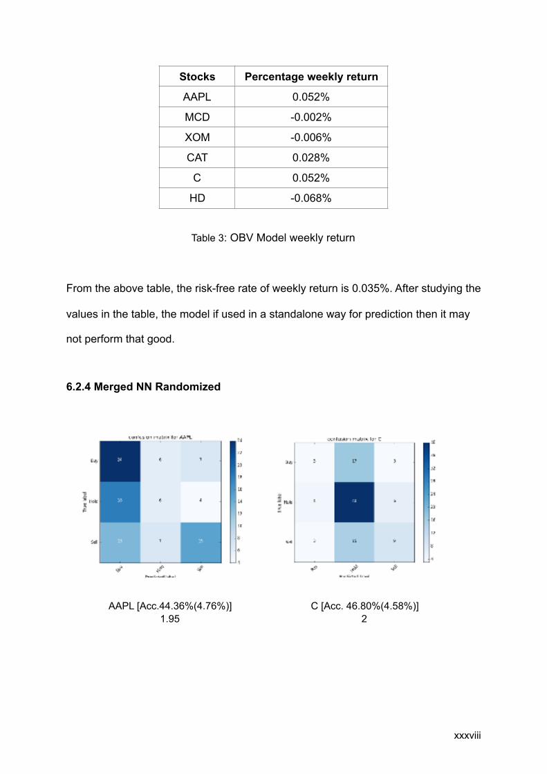
Table 3: OBV Model weekly return

From the above table, the risk-free rate of weekly return is 0.035%. After studying the

values in the table, the model if used in a standalone way for prediction then it may

not perform that good.

6.2.4 Merged NN Randomized

! !


AAPL 0.052%

MCD -0.002%

XOM -0.006%

CAT 0.028%

C 0.052%

HD -0.068%

!xxxviii

AAPL [Acc.44.36%(4.76%)] 1.95

C [Acc. 46.80%(4.58%)] 2

! !

Fig. 10: Merged NN Randomized Model Output

Discussion:





!xxxix

CAT [Acc.44.36%(4.76%)] 8.5

XOM [Acc.44.36%(4.76%)] 0.92

HD [Acc.34.26%(1.76%)] 0.90

MCD [Acc.33.36%(2.89%)] 1.42

Table 4: Merged NN Randomized Model weekly return

From the above table, the risk-free rate of weekly return is 0.035%. For this model, 4

out of 6 stocks are doing well

6.2.5 Merged NN in Sequence

! !


AAPL 0.19%

MCD 0.06%

XOM -0.001%

CAT 0.15%

C 0.06%

HD -0.03%

!xl

CAT [Acc.37.53%(3.72%)] 1.21

XOM [Acc.32.62%(2.46%)] 1.09

! !

! !

Fig. 11: Merged NN Sequence Model Output

Discussion:





!xli

HD [Acc.30.12%(2.36%)] 0.1

AAPL[Acc.26.22%(5.88%)] 0.22

C [Acc.31.62%(5.66%)] 0.9

MCD [Acc.29.62%(4.45%)] 0.1

Table 5: Merged NN Sequence Model weekly return

From the above table, it is evident that the moving average crossover model may

give positive returns from an investment. Also, after observing the ratio of the true

positive (buy and sell) and the false negative (buy and sell) of stock's confusion

matrix for the above model and values in the table, this model is not that efficient.

If the ratio of true positive to false negative is greater than one, the model behaves

relatively well and the investment may generate profit. If the ratio is less than zero,

the model results may be below average, and investment incurs a loss. It is evident

that sometimes model performs below average in real-world simulations. From the

confusion matrix results for the above simulations, Merged Model Randomized still

gives better results than the Merged Model in Sequence. If we consider only moving

average crossover model, then that model gives more returns than the rest of them.

Therefore, for future development one can surely use Moving average crossover

model as the starting base for prediction. Following section explains why some

models sometimes may perform poorly.


AAPL -0.38%

MCD -0.36%

XOM 0.001%

CAT 0.184%

C -0.01%

HD -0.18%

!xlii

Model Complexity

Model complexity is the measure of the set of hypotheses produced by a model. This

speculation is a guess that is made by design regarding the relationship between

dependent variable and input features. The complex nature of the model is directly

proportional to some hypotheses it can produce; larger the number more is the

complexity. Also, these hypothesize sets do not necessarily overlap. A model with

lesser complexity can provide better hypothesizes compared to the model belonging

to higher complexity. The same case is happening with ANN.

Generating good results using artificial neural network (ANN) architecture is very

challenging. Large number variables need to be configured and fine-tuned to get

expected results. It is a consuming task since one needs to decide many things like

agents to be included, the configuration of these agents, some hidden layers and the

nodes in each one of them. One additionally needs to analyze momentum

parameters and proper values of the learning rate to be used in back-propagation

algorithm. To thoroughly test such a large number of factors physically by

experimentation is nearly impossible since every variable adds another

measurement to the search space of possible ANN arrangements thus builds it

exponentially.

Training Data

Assume the complex nature of proposed models is workable, yet now perhaps the

issue can emerge because of the amount of training data that is available.

!xliii

The dataset used for training and testing above models had also been tested on

around 6,000 samples. These samples span for around 20 years. Even with this

amount of data, the model was performing poorly. This conclusion might be because

the stock markets are so unpredictable that they may require more information.

Market Noise

An analyst opinion is an expectation of a specific research firm on a specific stock.

For example, a substantial venture inquires about the company, for instance,

Samsung may issue a supposition on Apple stock. They may redesign or minimize

their assessments of capital execution and prescribe purchasing or offering the stock

at the present cost. The model does not know how the market may shift to reflect

analyst opinions. Numerous comparative traders may read these analyst feelings

before the market opens and are prepared to put in their requests when the market

opens quickly.

It is, hence, conceivable that the flag our model predicts may not relate to the cost of

the stock as it might have effectively moved to reflect expert sentiments and are no

longer significant. The calculation, for this situation, is adequately exchanging of the

insufficient data.

There are other sources of predicting value like to use the movement of assets

related to the S&P 500. Rather than foreseeing in light of yesterday's costs, the

model should anticipate given value changes in assets exchanged.

If above factors can predict the price trend, then the model built should be able to

utilize them.

!xliv

For above experiments, Buy signals strength is more accurate compared to Neutral

and Sell outputs. Utilizing the Buy flag and disregarding the Neutral and Sell signals

from the model, a time-based leave methodology can be actualized concentrating

fundamentally on a holding period and optionally on gainfulness. Utilizing the time-

based exit strategy, the model can set a precise measurement of time to be in a

trade. If set to two months, the model will leave two months in the wake of entering

the trade.

Using the Buy signal from the model and constraining the holding time to one week,

the algorithm implemented above can yield profitable results. Table 1 & 2 show the

percentage profit generated if the time-based exit strategy is carried out with Buy

signal strength.

With Sell & Neutral signals, the model can be used to implement Max Loss exit

strategy. The essential rule is if a trade plunges to a specific measure of indicated

loss, the model ought to exit the trade. There are two conventional approaches to

mechanize this sort of exit methodology: Stop Loss Orders and Stop Limit Orders.

Stop Loss Order: A request put with an agent to sell a security when it achieves a

specific cost

Example:

Suppose that given a Neutral flag, the model holds 100 shares of Apple Inc Stock

(Ticker: AAPL) at the cost of $25.00 per share. Presently, let us set that value, the

Max Loss on AAPL is to 10%. For this situation, the model can then instantly put in a

stop loss order at 10% beneath the value paid for AAPL, which, for this situation,

would be for $22.50. If AAPL somehow happened to drop in cost to $22.50, it would

!xlv

naturally trigger a request to sell the stock in the open market. By utilizing a stop loss

order, you can monitor your misfortunes and inside your hazard resilience.

!xlvi

Chapter 7

Conclusion

The most broadly utilized technical analysis methods demonstrated promising

outcomes in the investigations completed. A human using a technical indicator still

needs to make decisions based on experiences with trends for that indicator. We

have investigated a machine learning approach to capture this decision component

of using such an indicator.

It might have been expected that given the between correlation technical indicators

and the values of a stock that our results would have been a more positive. However,

just as humans have difficulties using indicators to accurately predict stocks, our

models also had to work to achieve results.

Machine learning methods offer the promise of discovering new metrics and/or

combinations of metrics from technical analysis, which do outperform the simple

technical analysis methods. However, our results showed that some of the more

complicated combinations of models actually underperform when compared to

neural networks based on a single indicator. This might be an overfit issue as the

size of the neural network is too large for the amount of data and nonlinear mapping

from input to output is over-complicated to converge rapidly. The moving average

crossover model it is showed the best results among the models we considered and

it can definitely be used it as a starting point for future research.

!xlvii

References

1. Yakup Kara, Melek Acar Boyacioglu, and Ömer Kaan Baykan. Predicting

direction of stock price index movement using artificial neural networks and

support vector machines: The sample of the Istanbul Stock Exchange. Expert

systems with Applications, 38(5):5311–5319, 2011.

2. Shunrong Shen, Haomiao Jiang, and Tongda Zhang. Stock market fore-

casting using machine learning algorithms, 2012.

3. E. F. Fama, K. R. French, "Common risk factors in the returns on stocks and

bonds", Journal of financial economics, vol. 33, no. 1, pp. 356, 1993.

4. D. G. McMillan, "Stock return dividend growth and consumption growth

predictability across markets and time: Implications for stock price

movement", International Review of Financial Analysis, vol. 35, pp. 90101,

2014.

5. M. Billah, S. Waheed and A. Hanifa, "Stock market prediction using an

improved training algorithm of neural network," 2016 2nd International

Conference on Electrical, Computer & Telecommunication Engineering

(ICECTE), Rajshahi, 2016, pp. 1-4.

6. M. D. Godfrey, C. W. Granger, and O. Morgenstern, "The random-walk

hypothesis of stock market behavioral," Kyklos, vol. 17, no. 1, pp. 1-30, 1964.

7. J. Murphy, "Technical analysis of the financial markets, prentice hall, London,"

1998

!xlviii

8. A. A. Bhat and S. S. Kamath, "Automated stock price prediction and trading

framework for Nifty intraday trading," 2013 Fourth International Conference on

Computing, Communications and Networking Technologies (ICCCNT),

Tiruchengode, 2013, pp. 1-6.

9. M. H. Pesaran, A. Timmermann, "Predictability of stock returns: Robustness

and economic significance", The Journal of Finance, vol. 50, no. 4, pp.

12011228, 1995

10.D. Avramov, "Stock return predictability and model uncertainty", Journal of

Financial Economics, vol. 64, no. 3, pp. 423458, 2002.

11. W. Lertyingyod and N. Benjamas, "Stock price trend prediction using Artificial

Neural Network techniques: Case study: Thailand stock exchange," 2016

International Computer Science and Engineering Conference (ICSEC),

Chiang Mai, 2016, pp. 1-6.

12.F. Andrade de Oliveira, L. Enrique Zárate, M. de Azevedo Reis and C. Neri

Nobre, "The use of artificial neural networks in the analysis and prediction of

stock prices," 2011 IEEE International Conference on Systems, Man, and

Cybernetics, Anchorage, AK, 2011, pp. 2151-2155.

13.Q. Mingyue, L. Cheng and S. Yu, "Application of the Artificial Neural Network

in Predicting the Direction of Stock Market Index," 2016 10th International

Conference on Complex, Intelligent, and Software Intensive Systems (CISIS),

Fukuoka, 2016, pp. 219-223

14.C. S. Vui, G. K. Soon, C. K. On, R. Alfred and P. Anthony, "A review of stock

market prediction with Artificial neural network (ANN)," 2013 IEEE

International Conference on Control System, Computing and Engineering,

Mindeb, 2013, pp. 477-482.

!xlix

15.W. Lertyingyod and N. Benjamas, "Stock price trend prediction using Artificial

Neural Network techniques: Case study: Thailand stock exchange," 2016

International Computer Science and Engineering Conference (ICSEC),

Chiang Mai, 2016, pp. 1-6.

16.Xiaohua Wang, P. K. H. Phua and Weidong Lin, "Stock market prediction

using neural networks: Does trading volume help in short-term prediction?,"

Proceedings of the International Joint Conference on Neural Networks, 2003.,

2003, pp. 2438-2442 vol.4.

17.K. Abhishek, A. Khairwa, T. Pratap and S. Prakash, "A stock market prediction

model using Artificial Neural Network," Computing Communication &

Networking Technologies (ICCCNT), 2012 Third International Conference on,

Coimbatore, 2012, pp. 1-5.]

18. R. E. Uhrig, Introduction to artificial neural networks, Proceedings of the 1995

IEEE IECON 21st International Conference on, vol. 1, pp.33- 37 vol. 1, 1995.

19.J. Zupan, Introduction to Artificial Neural Network (ANN) Methods: What They

Are and How to Use Them, Acta Chimica Slov, 41-327, 1994.

20.Predict the trend of stock prices using machine learning techniques a Seyed

Enayatolah Alavi, bHasanali Sinaei, c Elham Afsharirad

!l

Neural Net Stock Trend Predictor - SJSU Computer Science ...The Designated Project Committee...

Documents

Transcript of Neural Net Stock Trend Predictor - SJSU Computer Science ...The Designated Project Committee...