Network Design Methods Report - U.S. Fish and Wildlife Service
53
1 Determining Mitigation Needs for NiSource Natural Gas Transmission Facilities ‐ Implementation of the Multi‐Species Habitat Conservation Plan (MSHCP) Section 6 Cooperative Endangered Species Conservation Fund Grant (IDFW Subtask 1.3) Prepared by The Conservation Fund DECEMBER 2010 Network Design Methods Report
Transcript of Network Design Methods Report - U.S. Fish and Wildlife Service
1
Determining Mitigation Needs for NiSource Natural Gas Transmission Facilities ‐ Implementation of the Multi‐Species Habitat Conservation
Plan (MSHCP)
Section 6 Cooperative Endangered Species Conservation Fund Grant (IDFW Subtask 1.3)
Prepared by The Conservation Fund DECEMBER 2010
Network Design Methods Report

2
Network Design Methods Report
Table of Contents Network Design Methods ....................................................................................................................................................... 3
Green Infrastructure Network and Mitigation Planning Process Overview ........................................................................... 7
References ............................................................................................................................................................................ 11
Focal Species Analysis for Green Infrastructure Network Design Protocol .......................................................................... 12
Maxent Modeling of Mature Hardwood Forest ................................................................................................................... 28
Kentucky ............................................................................................................................................................................ 28
Ohio ................................................................................................................................................................................... 33
Pennsylvania ..................................................................................................................................................................... 41
Tennessee ......................................................................................................................................................................... 47

3
Network Design Methods The purpose of this report is to help decision makers, such as state officials and GIS technical staff, understand the steps taken in creating the Green Infrastructure Network for the NiSource MSHCP. For reference purposes, reports outlining the modeling of mature hardwood forests have been included, as well as the list of focal species and their thresholds that were reviewed for potential use in the project. It is anticipated that this report will serve as a convenient desk reference on Green Infrastructure and assist state officials in their current and future conservation planning initiatives. Green Infrastructure is technically defined as “a strategically planned and managed network of natural lands, working landscapes, and other open spaces that conserve ecosystem values and functions and provide associated benefits to human populations” (Benedict, McMahon 2006). Green infrastructure is a well established planning method that recognizes that limited resources are available to identify and protect the lands most suitable for conservation, and that competing interests, needs and opportunities must be evaluated to develop the most efficient and effective land conservation strategies. The green infrastructure approach has been utilized by numerous states and local communities within the NiSource service area (Weber, Wolf & Sloan, 2006; The Conservation Fund 2010). Green Infrastructure offers a conceptual approach for identifying mitigation opportunities at an ecosystem level. The Fund’s green infrastructure network prepared for this particular project extends well beyond NiSource’s 15,414 mile network to encompass the adjacent counties, ecoregions, and watershed units within the 14‐state area. Utilizing a green infrastructure approach provides NiSource, USFWS and the states a robust planning method to integrate species habitat mitigation within the context of an interconnected network of lands and waters, providing multiple benefits across the entire range of NiSource’s natural gas pipeline transmission activities. Such an approach will also ensure that a consistent methodology is used to determine selection of mitigation. The methodology employed in this process was accepted by the 14 participating states. The green infrastructure network was not used to determine how much mitigation should occur in response to a take, but rather, will be used to guide the types and locations for such mitigation opportunities at an ecosystem level. Green Infrastructure is based on the well‐established principles of landscape ecology and conservation biology (Forman and Godron, 1986; Ehrlich and Mooney, 1983). The network consists of core areas, corridors, and hubs that provide essential habitat to endangered and threatened species and that link to broader natural functions and processes at the ecosystem scale. Core areas contain well‐functioning natural ecosystems, and provide high‐quality habitat for native plants and animals that meet a minimum size threshold based on landscape conditions (see diagram). These are the nucleus of the green infrastructure network. Corridors are linear features that link core areas in order to allow animal and plant propagule movement between them with the goal of creating viable and persistent metapopulations. The landscape between core areas is assessed for its linkage potential, and conduits and barriers to wildlife and seed movement are identified. Corridor umbrella species can include reptiles, amphibians, fish, and mammals, depending on the type of linkage. Hubs are aggregations of core areas, other habitat, and other natural land, divided by major roads or gaps that meet a minimum size threshold based on landscape conditions. Hubs are intended to be large enough to support populations of
4
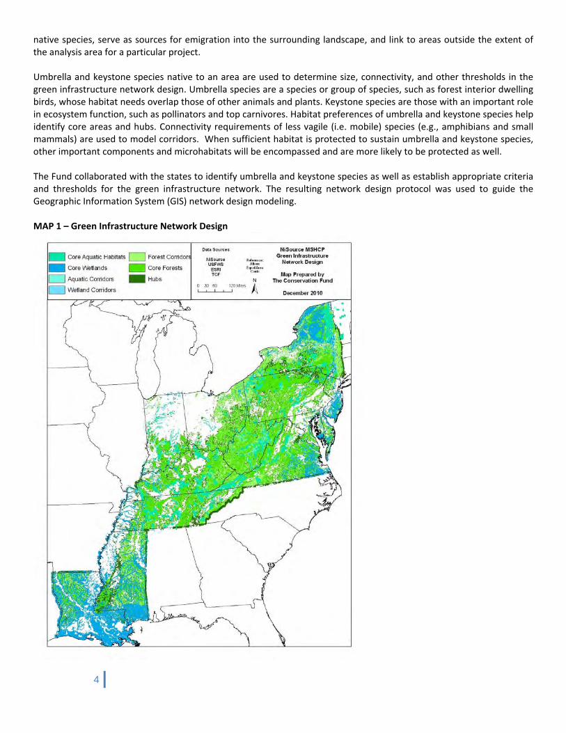
native species, serve as sources for emigration into the surrounding landscape, and link to areas outside the extent of the analysis area for a particular project. Umbrella and keystone species native to an area are used to determine size, connectivity, and other thresholds in the green infrastructure network design. Umbrella species are a species or group of species, such as forest interior dwelling birds, whose habitat needs overlap those of other animals and plants. Keystone species are those with an important role in ecosystem function, such as pollinators and top carnivores. Habitat preferences of umbrella and keystone species help identify core areas and hubs. Connectivity requirements of less vagile (i.e. mobile) species (e.g., amphibians and small mammals) are used to model corridors. When sufficient habitat is protected to sustain umbrella and keystone species, other important components and microhabitats will be encompassed and are more likely to be protected as well. The Fund collaborated with the states to identify umbrella and keystone species as well as establish appropriate criteria and thresholds for the green infrastructure network. The resulting network design protocol was used to guide the Geographic Information System (GIS) network design modeling. MAP 1 – Green Infrastructure Network Design

5
Green Infrastructure Network Design Elements The Fund collaborated with the states on the selection of core habitats for the 14‐state area. For this project, forests, wetlands, and aquatic systems were selected given the landscape characteristics of the area. Cave and karst systems also were analyzed, but mostly were addressed through species modeling work completed for the Indiana Bat (Myotis sodalis) and Madison Cave Isopod (Antrolana lira). Mapping these core habitats helped visualize an interconnected network of forests, wetlands, and aquatic systems where mitigation projects could be strategically implemented to meet the requirements of the MSHCP that also advanced other conservation objectives. Core Forests are contiguous areas of relatively undisturbed, mature forest with a minimum size threshold based on landscape conditions. For a current green infrastructure project ongoing in Maryland, core forest areas had to include forest blocks with at least 247 acres (100 hectares) of mature interior deciduous or mixed forest habitat that provided habitat for a majority of forest interior dwelling birds in the study area. Core Wetlands are contiguous natural areas with relatively undisturbed wetlands that meet a minimum size threshold based on landscape conditions. For a recent green infrastructure project in Delaware, core wetland areas had to be at least 25 acres (10 hectares) in size and include habitat for umbrella species dependent upon riparian forest (Louisiana waterthrush, wood turtle), forested wetlands (Prothonotary warbler), wetland‐forest complexes (amphibians, turtles), and/or marsh (Least bittern). Core Aquatic Systems contain a threshold amount of relatively unimpaired streams based on landscape conditions plus associated riparian forest and wetlands. Umbrella species for aquatic systems often include fish, mussels, and benthic macroinvertebrates. For a recent green infrastructure project in Delaware, core aquatic systems had to contain at least a kilometer of streams with minimal impacts from channelization, dams, and road culverts. These core areas were combined with corridor and hub areas to create a characterized green infrastructure network map that shows the overlap of the core habitats. Core areas are not mutually exclusive. In fact, the overlap of core areas demonstrates locations where protection of natural systems will likely benefit numerous species that may be dependent on multiple landscape types throughout their life cycle.

6
MAP 2 ‐ Characterized Green Infrastructure Network
7
Green Infrastructure Network and Mitigation Planning Process Overview This overview provided a detailed look at the green infrastructure methods, assumptions and critical feedback from state agencies during the planning process. One of the first adjustments to the project was the study area. While the MSHCP study area is 14 states, over time it became clear that the amount of pipeline in North Carolina was minimal, and the list of species covered by the MSHCP did not warrant a green infrastructure approach. The formal study area for the green infrastructure network was reduced to 13 states, with North Carolina involved on a consultation basis. Between October and December 2008, the Fund completed 12 focus group meetings. Over 116 state agency staff and other stakeholders participated in the focus group meetings providing valuable information. Following a short presentation on the green infrastructure design method, the Fund staff distributed a six‐page feedback form to solicit information on current species distribution, current research and fieldwork, and species that were no longer present within the state. Participants were also asked for comments on focal species, criteria and thresholds for core areas for forest, wetlands, aquatics, and karst landscape types. Similar questions were listed for feedback on assumptions for the delineation of wildlife corridors. Participants were requested to comment on the extent of the proposed study area for the green infrastructure network. The feedback forms were designed to obtain precise information that would be delivered in a useful manner to the Fund design team and reduce the possibilities of misunderstandings. Facilitators carefully guided participants through each section of the feedback forms to make sure that terms where understood and the concepts were well illustrated and to pause for any questions. Participants made extensive comments on all aspects of the green infrastructure effort. Next, participants were asked to review a GIS data quality assessment report and a bibliography of state planning documents. Participants were asked to add missing GIS layers or planning documents that were in development so that these products could be incorporated into the NiSource planning effort. The Fund transcribed and analyzed the input provided at the state focus group meetings. During this period, the Fund staff continued to contact individual focus group participants to obtain additional GIS layers, scientific literature, or clarification of comments made on the input forms. On February 3, 2009, the Fund sent a follow‐up note to the state points of contact, updating staff officials on the activities since the focus group meetings. A general project time line was provided to state officials on the expected delivery of the green infrastructure protocol. The protocol document defines scales, establishes criteria and thresholds, identifies keystone/umbrella species, and outlines green infrastructure network elements (e.g. core forests, core wetlands, core aquatic systems, core cave/karst systems, hubs, corridors). On May 12, 2009, the Fund sent the state points of contact a sample or preliminary draft protocol for review and comment. The Fund received comments from state officials from Indiana and Virginia on the preliminary draft green infrastructure protocol. Based on feedback from focus group meetings from the spring and the review of the preliminary draft green infrastructure network protocol, the Fund staff created a comprehensive draft protocol, also known as a Network Design Package, for each state. The Network Design Package explained in detail how the green infrastructure network would be created, how it may be adjusted to fit particular state needs, how it interfaces with other state programs, and how it will relate to the upcoming task of identifying and characterizing potential mitigation opportunities for the NiSource MSHCP. The network design methods included approaches that will be standardized across the study area and those that will be state‐specific. The draft protocol features: (1) a comprehensive bibliography of relevant planning documents for each state, (2) tailored

8
information for each state on how the GI network relates to current state planning initiatives, including the State Wildlife Action Plan, and (3) a preview of the upcoming mitigation site report and decision support framework task. The heart of the Network Design Package was the network methods section that described, in an outline form and with a series of spreadsheets, the steps in designing core areas, hubs and corridors for each state. To create the outline, the Fund staff conducted an extensive literature review of all NiSource take species as well as focal species for each eco‐system and landscape feature. In addition, the Fund researched the species recommended as focal species by state officials from the earlier state meetings in 2008. By March 2009, a master species spreadsheet was created highlighting over 314 animal species and their home ranges, minimum preserve size, dispersal distance, separation distance for suitable habitat, separation distance for unsuitable habitat, descriptions of dispersal barriers and dispersal conduits and whether the species was a prime candidate to serve as either an indicator or keystone species. A similar worksheet was created for nine plant species as well. Species that were determined to be appropriate focal species were analyzed further in worksheets summarizing their habitat needs and thresholds for core areas, hubs and corridors. These spreadsheets provide invaluable information for state agencies, as they have great use beyond the NiSource Green Infrastructure Network. As state agencies attempt to update their Wildlife Action Plan or address the impact of climate change, the focal species spread sheets provide a great starting point for additional modeling and planning work. In addition, within the Network Methods section was a summary of GIS models that would be used including maximum entropy (Maxent – Dudik, Phillips, and Schapire, 2008), functional connectivity (FunConn ‐ Theobald, Norman, and Sherburne, 2006), and least cost path. Maxent is a machine learning technique that can be used to predict the geographic distribution of animal or plant species or other entities of interest (Phillips, Anderson, and Schapire, 2006). Maxent compares a set of samples from a distribution over a defined space, such as recorded locations of a particular species, to a set of features, such as relevant environmental variables, over that same space. The FunConn modeling toolbox for ArcGIS™ provides a spatial context for wildlife species, using graph theory approaches to define functional habitat patches and landscape connectivity. Included in the report was a trial run of a Maxent model and FunConn model of the Indiana Bat (Myotis sodalis) for the Upper Wabash River Watershed in Indiana. On July 2, 2009, the Fund sent the first draft protocol document to the state of Indiana. Throughout July, each state point of contact received the tailored Network Design Protocol for review, and comments were provided to the Fund between July and September 2009. The process for modeling the 13‐state green infrastructure network was complex and lengthy. Many details of the modeling processes and assumptions are covered in the Green Infrastructure Network Protocol document that was generated and tailored for each state. A summary of the focal species analysis completed for the green infrastructure network design protocol is provided at the end of this summary report. The following narrative highlights major steps within the overall project timeline. Starting in the spring of 2010, the Fund staff identified core areas, hubs and corridors of the green infrastructure network. Staff divided the landscape into forest, wetland and aquatic systems, and identified core areas and corridors in each system. The wetland core areas were completed in May 2010, and associated wetland corridors were delineated in August 2010. Staff relied on the National Land Cover Database’s wetland classes, as this was the only data consistently available across all 13 states. Based on peer‐reviewed literature on habitat needs of focal species, wetlands that were greater than or equal to 370 acres (150 hectares) were selected as core wetland areas. Wetland connectors were manually identified using National Hydrographic Data (NHD) in three NHD regions (2, 5, and 6). Staff added the stream valleys and riparian cover along these connector streams to identify wetland corridors. Modeling work on the forest core areas was begun in March 2010 and completed in September 2010 for the 13‐state study area. The Fund used the “National Green Infrastructure Assessment” developed by the United States Environmental Protection Agency (EPA). This assessment uses a morphological spatial patter analysis (MSPA) to identify hubs and links. The Fund used the assessment GIS layer on forest cores as a foundation, building upon this work and extending its usefulness. To provide an ecological context for the analysis, the Fund extracted forest cores from the

9
National GI Assessment using ecoregions as a template. The Fund examined many different ecoregions across the 13‐state area. The largest ecoregion within the network was the Interior Plateau – covering 43,033 square miles and the smallest ecoregion was the Mississippi River Alluvial Plain, which covers 1,029 square miles. Next, the Fund examined the peer‐reviewed literature on focal species, and with feedback from state officials, created a matrix of focal species with acreage thresholds matched to both state boundaries and ecoregions. By using ecoregion boundaries, the Fund was able to cross reference each ecoregion to a suite of focal species and consequentially to a size threshold needed to sustain a viable population of those species. These thresholds indicate the minimal forest acreage that can accommodate the needs of many forest‐dependent species. A caveat on the interpretation of focal species thresholds is that this method is an attempt to broadly characterize a landscape and does not mean that these species actually occupy these forest core areas. Focal species thresholds are board indicators, providing general clues as to ecoregion habitat quality and viability. The Fund was unable to obtain sufficient focal species location data to perform Maxent modeling, but the core focal species and habitat associations were part of the network design goals. Several examples of the use of focal species thresholds may help illustrate the value of the effort. For the Western Allegheny Plateau, the fourth largest ecoregion covering 31,445 square miles, the Fund selected a suite of five bird species with a minimum acreage threshold of between 24 to 37 acres to outline core areas for scrub and early successional forests. Several ecoregions shared focal species. A suite of 16 birds, including the Scarlet Tanager, Oven Bird and Kentucky Warbler, was used to characterize mature broadleaf forests across eight ecoregions. Patches selected were above 247 acres (100 hectares) and optimal forest block size was 9,889 acres (4,000 hectares). The Fund provided “value added” to the EPA National GI Assessment, enhancing its overall quality by incorporating species thresholds to select the suitable forest core areas. In September 2010, the Fund began using a least cost path model to identify optimal connections between core forest areas, preferring intervening forest and avoiding urban areas and roads. Due to the large 13 state‐study area and complexity of the model, more than two months was required to identify least cost paths to connect core forest. As least cost path models provide simple linear connection between core areas, additional time was required to provide buffers for these linear features to a proper size to serve as wildlife corridors. Forest corridors were at least 656 feet (200 meters) wide, based on interior forest bird requirements and a study that showed that corridors greater than 656 feet (200 meters) wide generally had less than 10% exotic invasive plants. A width of 984 feet (300 meters) was preferable. Aquatic core areas were completed in August 2010 with stream corridors outlined in September. Staff ran four different iterations of core streams, adjusting the methodology each time to improve model output. The Fund identified catchments containing freshwater mussels, which are generally sensitive to flow stability and water quality. Staff added brook trout streams with a Population Integrity score of 10 or greater, using Trout Unlimited’s Conservation Success Index. In addition, state specific priority layers were used such as Kentucky’s Priority Watersheds for Conservation of Imperiled Fishes and Mussels, Tennessee’s Aquatic Priority Habitat, New Jersey’s mussel streams from its Landscape 3.0 planning process, native brook trout streams in West Virginia, and catchments containing viable populations of Nashville Crayfish (Orconectes shoupi). The Fund discarded catchments with less than 5% impervious cover. This threshold captured 99% of the freshwater mussel occurrences in the Ohio River drainage. Stream segments with acid mine drainage, impoundments, channelized, or classified as intermittent streams, were also removed. Finally, core streams had to run at least 6.2 miles (10km) with suitable conditions, as described above. Concurrent to the analysis on core areas, the Fund modeled hubs for the overall green infrastructure network. Hubs are large contiguous blocks of land that contain core areas. Hubs are intended to be large enough to support populations of native species, and serve as sources for emigration by species into the surrounding landscape, as well as providing other ecosystem services like clean air, water, and recreation opportunities. Frequently hubs include working lands such as commercial timber lands and farmlands, and require a collaborative approach to conservation success. As hubs provide

10
a protective buffer around core areas, a critical step in creating the hubs was buffering the core forest, wetland and stream areas to include edge transitions and protection from disturbances and pollution. Next, staff added modeled Indiana bat summer habitat, Indiana bat hibernacula plus a 10 mile buffer, modeled mussel stream reaches plus a 328‐foot buffer (100 meters), modeled Nashville crayfish reaches plus a 328‐foot buffer, modeled Madison cave isopod (Antrolana lira) habitat in Virginia, known Madison cave isopod locations in West Virginia, and occupied Louisiana black bear (Ursus americanus luteolus) habitat. The Fund also added rare species and community occurrences from state Natural Heritage Programs and applied a 328‐foot buffer to these locations. Staff also included state priority areas like Large Forest Tracts (>1,000 acres) in Kentucky (although these would also be included in core forest), NY Natural Heritage Important Areas, NY Important Bird Areas, Ohio caves, TN Natural Areas, and TN Very High or High Priority aquatic, terrestrial, and subterranean habitat. The Fund modeled occurrences of mature broadleaf forest for part of the study area. In the eastern United States, mature hardwood forest provides habitat for many species of native flora and fauna, but is much less common now than historically. We performed pilot modeling in Charles County, Maryland, where we compared fine‐scale geographic data available locally to coarse‐scale data available nationally. As expected, a model constructed with the best locally available data, including LiDAR‐derived canopy height and fine‐scale soil maps, outperformed a model constructed with nationally consistent data. However, the model using national data nevertheless accurately identified most mature hardwood forest sites and excluded most young forest. We then applied the coarse‐scale approach to four states: Pennsylvania, Ohio, Kentucky, and Tennessee. Average test AUC (area under the receiver operating curve) based on 10 replicates varied from 0.76 to 0.80 when comparing mature hardwood forest locations to general forest locations. The maximum training or test sensitivity plus specificity threshold, depending on the state, captured 78‐79% of positive locations while rejecting 74‐81% of negative locations, and covered 5‐9% of the states. Next, staff removed developed and barren land, along with major roads. Finally, staff removed tendrils and small patches less than 247 acres (100 hectares). The final hubs were then compared to state‐specific analogues in Delaware and Maryland to assess the modeling accuracy. Because the NiSource hubs utilized GIS layers common to the entire 13‐state study area there were not as many hubs as the state specific green infrastructure plans had highlighted since those smaller scale plans utilized more detailed data and in‐depth analyses. However, as the size of the hubs increased, there was a greater level of agreement between state level plans and the NiSource green infrastructure network on hubs, confirming integrity and accuracy of the analysis. In late September 2010, the Fund planning team met in North Carolina to integrate the last state agency comments into the decision trees. At this time, the process for characterizing the green infrastructure network was discussed. As green infrastructure networks are vast, additional analysis often is needed to prioritize areas within the network, so that the high quality or most vulnerable resources are conserved first. The green infrastructure network is a collection of many different parts, and the network characterization focuses on prioritizing the areas of the network that serve the greatest number of different benefits. For example, a network section that was a core aquatic area, served as a corridor and was part of a hub would be a higher priority in the network than would a section that was just a hub. The network characterization results were included in the decision trees to help decision makers compare the value of projects within the green infrastructure network.

11
References Benedict, M.A. and E.T. McMahon. 2006. Green Infrastructure: Linking Landscapes and Communities. Island Press, Washington, DC. 299 pp. Conservation Fund, The. 2010. Projects: Mid‐Atlantic, Southeast, Midwest. Green Infrastructure.net. In, http://www.greeninfrastructure.net/projects Dudik, M., S. Phillips, and R. Schapire. 2008. Maxent, Version 3.2.19. http://www.cs.princeton.edu/~schapire/Maxent/ Ehrlich, P. R. and H. A. Mooney. 1983. Extinction, substitution, and ecosystem services. BioScience. 33(4):248‐254 Forman, R. T. T. and M. Godron. 1986. Landscape Ecology. John Wiley and Sons, New York, NY. 619 pp. Phillips, Steven J., Robert P. Anderson, and Robert E. Schapire. 2006. Maximum entropy modeling of species geographic distributions. Ecological Modelling, 190:231‐259. Spatial Ecology. 2010. Hawth’s Tools for ArcGIS. http://www.spatialecology.com/htools/overview.php Theobald, D. M., J. B. Norman, and M. R. Sherburne. 2006. ArcGIS tools for functional connectivity modeling. Natural Resource Ecology Laboratory, Colorado State University, Fort Collins, CO. http://www.nrel.colostate.edu/projects/starmap/funconn_index.htm Weber, T., J. Wolf, and A. Sloan. 2006. Maryland’s green infrastructure assessment: development of a comprehensive approach to land conservation. Landscape and Urban Planning. 77:94‐110.
12
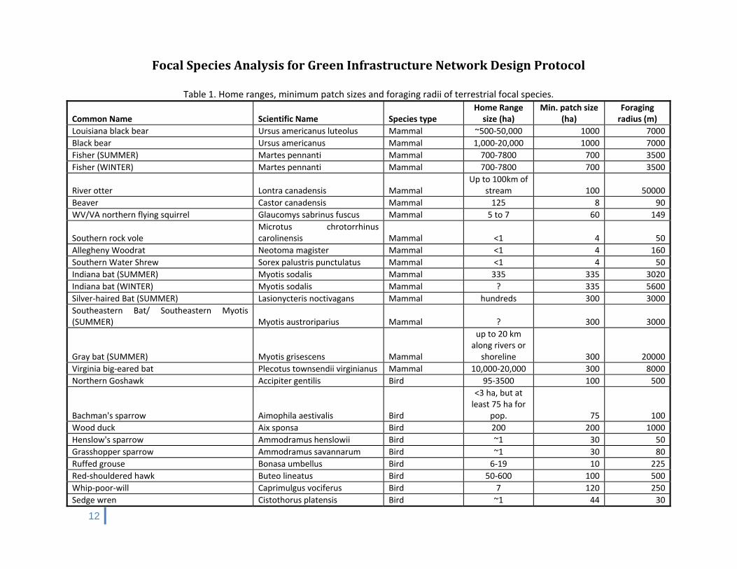
Focal Species Analysis for Green Infrastructure Network Design Protocol
Table 1. Home ranges, minimum patch sizes and foraging radii of terrestrial focal species.
Common Name Scientific Name Species type Home Range size (ha)
Min. patch size (ha)
Foraging radius (m)
Louisiana black bear Ursus americanus luteolus Mammal ~500‐50,000 1000 7000
Black bear Ursus americanus Mammal 1,000‐20,000 1000 7000
Fisher (SUMMER) Martes pennanti Mammal 700‐7800 700 3500
Fisher (WINTER) Martes pennanti Mammal 700‐7800 700 3500
River otter Lontra canadensis MammalUp to 100km of
stream 100 50000
Beaver Castor canadensis Mammal 125 8 90
WV/VA northern flying squirrel Glaucomys sabrinus fuscus Mammal 5 to 7 60 149
Southern rock vole Microtus chrotorrhinus carolinensis Mammal <1 4 50
Allegheny Woodrat Neotoma magister Mammal <1 4 160
Southern Water Shrew Sorex palustris punctulatus Mammal <1 4 50
Indiana bat (SUMMER) Myotis sodalis Mammal 335 335 3020
Indiana bat (WINTER) Myotis sodalis Mammal ? 335 5600
Silver‐haired Bat (SUMMER) Lasionycteris noctivagans Mammal hundreds 300 3000
Southeastern Bat/ Southeastern Myotis (SUMMER) Myotis austroriparius Mammal ? 300 3000
Gray bat (SUMMER) Myotis grisescens Mammal
up to 20 km along rivers or
shoreline 300 20000
Virginia big‐eared bat Plecotus townsendii virginianus Mammal 10,000‐20,000 300 8000
Northern Goshawk Accipiter gentilis Bird 95‐3500 100 500
Bachman's sparrow Aimophila aestivalis Bird
<3 ha, but at least 75 ha for
pop. 75 100
Wood duck Aix sponsa Bird 200 200 1000
Henslow's sparrow Ammodramus henslowii Bird ~1 30 50
Grasshopper sparrow Ammodramus savannarum Bird ~1 30 80
Ruffed grouse Bonasa umbellus Bird 6‐19 10 225
Red‐shouldered hawk Buteo lineatus Bird 50‐600 100 500
Whip‐poor‐will Caprimulgus vociferus Bird 7 120 250
Sedge wren Cistothorus platensis Bird ~1 44 30

13
Common Name Scientific Name Species type Home Range size (ha)
Min. patch size (ha)
Foraging radius (m)
Black‐throated blue warbler Dendroica caerulescens Bird 2 1100 90
Cerulean warbler Dendroica cerulea Bird 1‐2
4000 (but may be >250‐3000
in MD or >1600 in TN) 60
Prairie warbler Dendroica discolor Bird ~1 10 70
Yellow warbler Dendroica petechia Bird <1 4 50
Pine warbler Dendroica pinus Bird ~1 30 60
Acadian flycatcher Empidonax virescens Bird 2‐3 38 90
Worm‐eating warbler Helmitheros vermivorum Bird 2‐5 300 120
Black‐necked stilt Himantopus mexicanus Bird 10‐60 10 400
Wood thrush Hylocichla mustelina Bird 1‐3 100 90
Yellow‐breasted chat Icteria virens Bird 1‐3 5 90
Least bittern Ixobrychus exilis Bird 1 5 60
Kentucky warbler Oporornis formosus Bird 1 130 60
Northern parula Parula americana Bird <1 100 60
Savannah sparrow Passerculus sandwichensis Bird 0.05 to 1.25 100 60
Red cockaded woodpecker Picoides borealis Bird 15‐225 40 850
Prothonotary warbler Protonotaria citrea Bird <1 100 60
King rail Rallus elegans Bird0.4 to 3.6 ha (breeding) 60 100
American woodcock Scolopax minor Bird 71 100? 230
Ovenbird Seiurus aurocapilla Bird 1‐2 100 70
Louisiana waterthrush Seiurus motacilla Bird 2.5 100 90
Barred owl Strix varia Bird 86‐369 100 1000
Eastern meadowlark Sturnella magna Bird 3 8 100
Golden‐winged warbler Vermivora chrysoptera Bird 1‐2 10 80
Blue‐winged warbler Vermivora pinus Bird 1 1 60
Yellow‐throated vireo Vireo flavifrons Bird 1.5 100 70
White‐eyed vireo Vireo griseus Bird 1‐2 28 80
Hooded warbler Wilsonia citrina Bird 0.75 200 50
Bog turtle Glyptemys muhlenbergii Reptile 0.2‐1.3 <1 60
Spotted turtle Clemmys guttata Reptile 2 to 3 3.5 300
Wood turtle Glyptemys insculpta Reptile<2 km along streams 28 900
Timber Rattlesnake Crotalus horridus Reptile 200 4000 3600
Copperbelly watersnake Nerodia erythrogaster neglecta Reptile 20 200 250
14
Common Name Scientific Name Species type Home Range size (ha)
Min. patch size (ha)
Foraging radius (m)
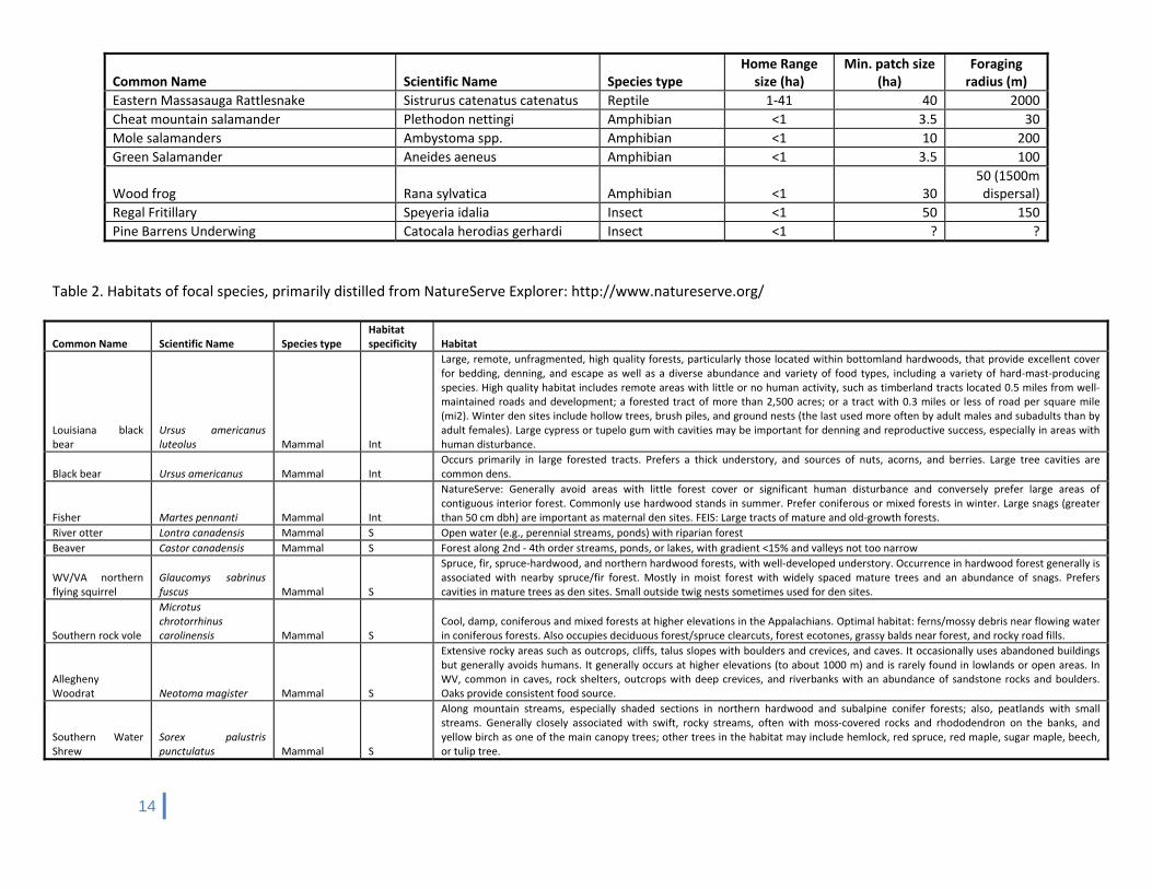
Eastern Massasauga Rattlesnake Sistrurus catenatus catenatus Reptile 1‐41 40 2000
Cheat mountain salamander Plethodon nettingi Amphibian <1 3.5 30
Mole salamanders Ambystoma spp. Amphibian <1 10 200
Green Salamander Aneides aeneus Amphibian <1 3.5 100
Wood frog Rana sylvatica Amphibian <1 30 50 (1500m dispersal)
Regal Fritillary Speyeria idalia Insect <1 50 150
Pine Barrens Underwing Catocala herodias gerhardi Insect <1 ? ?
Table 2. Habitats of focal species, primarily distilled from NatureServe Explorer: http://www.natureserve.org/
Common Name Scientific Name Species type Habitat specificity Habitat
Louisiana black bear
Ursus americanus luteolus Mammal Int
Large, remote, unfragmented, high quality forests, particularly those located within bottomland hardwoods, that provide excellent cover for bedding, denning, and escape as well as a diverse abundance and variety of food types, including a variety of hard‐mast‐producing species. High quality habitat includes remote areas with little or no human activity, such as timberland tracts located 0.5 miles from well‐maintained roads and development; a forested tract of more than 2,500 acres; or a tract with 0.3 miles or less of road per square mile (mi2). Winter den sites include hollow trees, brush piles, and ground nests (the last used more often by adult males and subadults than by adult females). Large cypress or tupelo gum with cavities may be important for denning and reproductive success, especially in areas with human disturbance.
Black bear Ursus americanus Mammal Int Occurs primarily in large forested tracts. Prefers a thick understory, and sources of nuts, acorns, and berries. Large tree cavities are common dens.
Fisher Martes pennanti Mammal Int
NatureServe: Generally avoid areas with little forest cover or significant human disturbance and conversely prefer large areas of contiguous interior forest. Commonly use hardwood stands in summer. Prefer coniferous or mixed forests in winter. Large snags (greater than 50 cm dbh) are important as maternal den sites. FEIS: Large tracts of mature and old‐growth forests.
River otter Lontra canadensis Mammal S Open water (e.g., perennial streams, ponds) with riparian forest
Beaver Castor canadensis Mammal S Forest along 2nd ‐ 4th order streams, ponds, or lakes, with gradient <15% and valleys not too narrow
WV/VA northern flying squirrel
Glaucomys sabrinus fuscus Mammal S
Spruce, fir, spruce‐hardwood, and northern hardwood forests, with well‐developed understory. Occurrence in hardwood forest generally is associated with nearby spruce/fir forest. Mostly in moist forest with widely spaced mature trees and an abundance of snags. Prefers cavities in mature trees as den sites. Small outside twig nests sometimes used for den sites.
Southern rock vole
Microtus chrotorrhinus carolinensis Mammal S
Cool, damp, coniferous and mixed forests at higher elevations in the Appalachians. Optimal habitat: ferns/mossy debris near flowing water in coniferous forests. Also occupies deciduous forest/spruce clearcuts, forest ecotones, grassy balds near forest, and rocky road fills.
Allegheny Woodrat Neotoma magister Mammal S
Extensive rocky areas such as outcrops, cliffs, talus slopes with boulders and crevices, and caves. It occasionally uses abandoned buildings but generally avoids humans. It generally occurs at higher elevations (to about 1000 m) and is rarely found in lowlands or open areas. In WV, common in caves, rock shelters, outcrops with deep crevices, and riverbanks with an abundance of sandstone rocks and boulders. Oaks provide consistent food source.
Southern Water Shrew
Sorex palustris punctulatus Mammal S
Along mountain streams, especially shaded sections in northern hardwood and subalpine conifer forests; also, peatlands with small streams. Generally closely associated with swift, rocky streams, often with moss‐covered rocks and rhododendron on the banks, and yellow birch as one of the main canopy trees; other trees in the habitat may include hemlock, red spruce, red maple, sugar maple, beech, or tulip tree.
15
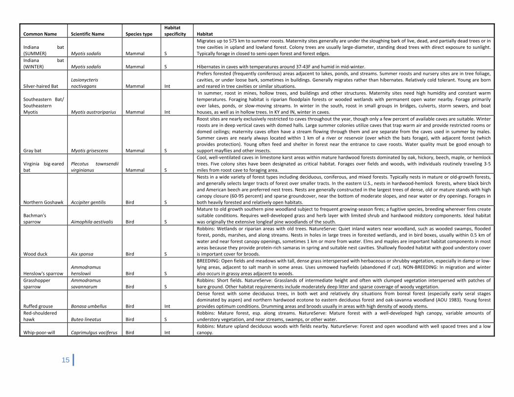
Common Name Scientific Name Species type Habitat specificity Habitat
Indiana bat (SUMMER) Myotis sodalis Mammal S
Migrates up to 575 km to summer roosts. Maternity sites generally are under the sloughing bark of live, dead, and partially dead trees or in tree cavities in upland and lowland forest. Colony trees are usually large‐diameter, standing dead trees with direct exposure to sunlight. Typically forage in closed to semi‐open forest and forest edges.
Indiana bat (WINTER) Myotis sodalis Mammal S Hibernates in caves with temperatures around 37‐43F and humid in mid‐winter.
Silver‐haired Bat Lasionycteris noctivagans Mammal Int
Prefers forested (frequently coniferous) areas adjacent to lakes, ponds, and streams. Summer roosts and nursery sites are in tree foliage, cavities, or under loose bark, sometimes in buildings. Generally migrates rather than hibernates. Relatively cold tolerant. Young are born and reared in tree cavities or similar situations.
Southeastern Bat/ Southeastern Myotis Myotis austroriparius Mammal Int
In summer, roost in mines, hollow trees, and buildings and other structures. Maternity sites need high humidity and constant warm temperatures. Foraging habitat is riparian floodplain forests or wooded wetlands with permanent open water nearby. Forage primarily over lakes, ponds, or slow‐moving streams. In winter in the south, roost in small groups in bridges, culverts, storm sewers, and boat houses, as well as in hollow trees. In KY and IN, winter in caves.
Gray bat Myotis grisescens Mammal S
Roost sites are nearly exclusively restricted to caves throughout the year, though only a few percent of available caves are suitable. Winter roosts are in deep vertical caves with domed halls. Large summer colonies utilize caves that trap warm air and provide restricted rooms or domed ceilings; maternity caves often have a stream flowing through them and are separate from the caves used in summer by males. Summer caves are nearly always located within 1 km of a river or reservoir (over which the bats forage), with adjacent forest (which provides protection). Young often feed and shelter in forest near the entrance to cave roosts. Water quality must be good enough to support mayflies and other insects.
Virginia big‐eared bat
Plecotus townsendii virginianus Mammal S
Cool, well‐ventilated caves in limestone karst areas within mature hardwood forests dominated by oak, hickory, beech, maple, or hemlock trees. Five colony sites have been designated as critical habitat. Forages over fields and woods, with individuals routinely traveling 3‐5 miles from roost cave to foraging area.
Northern Goshawk Accipiter gentilis Bird S
Nests in a wide variety of forest types including deciduous, coniferous, and mixed forests. Typically nests in mature or old‐growth forests, and generally selects larger tracts of forest over smaller tracts. In the eastern U.S., nests in hardwood‐hemlock forests, where black birch and American beech are preferred nest trees. Nests are generally constructed in the largest trees of dense, old or mature stands with high canopy closure (60‐95 percent) and sparse groundcover, near the bottom of moderate slopes, and near water or dry openings. Forages in both heavily forested and relatively open habitats.
Bachman's sparrow Aimophila aestivalis Bird S
Mature to old growth southern pine woodland subject to frequent growing‐season fires; a fugitive species, breeding wherever fires create suitable conditions. Requires well‐developed grass and herb layer with limited shrub and hardwood midstory components. Ideal habitat was originally the extensive longleaf pine woodlands of the south.
Wood duck Aix sponsa Bird S
Robbins: Wetlands or riparian areas with old trees. NatureServe: Quiet inland waters near woodland, such as wooded swamps, flooded forest, ponds, marshes, and along streams. Nests in holes in large trees in forested wetlands, and in bird boxes, usually within 0.5 km of water and near forest canopy openings, sometimes 1 km or more from water. Elms and maples are important habitat components in most areas because they provide protein‐rich samaras in spring and suitable nest cavities. Shallowly flooded habitat with good understory cover is important cover for broods.
Henslow's sparrow Ammodramus henslowii Bird S
BREEDING: Open fields and meadows with tall, dense grass interspersed with herbaceous or shrubby vegetation, especially in damp or low‐lying areas, adjacent to salt marsh in some areas. Uses unmowed hayfields (abandoned if cut). NON‐BREEDING: In migration and winter also occurs in grassy areas adjacent to woods.
Grasshopper sparrow
Ammodramus savannarum Bird S
Robbins: Short fields. NatureServe: Grasslands of intermediate height and often with clumped vegetation interspersed with patches of bare ground. Other habitat requirements include moderately deep litter and sparse coverage of woody vegetation.
Ruffed grouse Bonasa umbellus Bird Int
Dense forest with some deciduous trees, in both wet and relatively dry situations from boreal forest (especially early seral stages dominated by aspen) and northern hardwood ecotone to eastern deciduous forest and oak‐savanna woodland (AOU 1983). Young forest provides optimum conditions. Drumming areas and broods usually in areas with high density of woody stems.
Red‐shouldered hawk Buteo lineatus Bird S
Robbins: Mature forest, esp. along streams. NatureServe: Mature forest with a well‐developed high canopy, variable amounts of understory vegetation, and near streams, swamps, or other water.
Whip‐poor‐will Caprimulgus vociferus Bird Int Robbins: Mature upland deciduous woods with fields nearby. NatureServe: Forest and open woodland with well spaced trees and a low canopy.

16
Common Name Scientific Name Species type Habitat specificity Habitat
Sedge wren Cistothorus platensis Bird Int
Grasslands and savanna, especially where wet or boggy; sedge marshes; moist meadows with scattered low bushes; upland margins of ponds and marshes; coastal brackish marshes of cordgrass, herbs, and low shrubs. Avoids cattail marshes. Preferred habitats in tidewater areas in MD consisted of switchgrass meadows along the inner margins of tidal marshes. In the Allegheny Mountains of MD, sedge meadows in boreal bogs were usually occupied, whereas orchard grass pastures and hayfields were used at upland sites elsewhere in the state.
Black‐throated blue warbler
Dendroica caerulescens Bird S Large areas of interior forest, with dense, well‐developed shrub layer
Cerulean warbler Dendroica cerulea Bird S Large tracts of mature, semi‐open deciduous interior forest, particularly in floodplains or other mesic conditions. In MD, rarely nests in forest <250 ha; in TN, not found in forest <1600 ha. TN DNR: not found within 1/4 mile of clearcut.
Prairie warbler Dendroica discolor Bird Int Scrub‐shrub or early successional forest
Yellow warbler Dendroica petechia Bird G Open scrub, second‐growth woodland, thickets, farmlands and gardens, especially near water. (note: IN and OH focal species only)
Pine warbler Dendroica pinus Bird S Highest densities in pine forest at least 40 years old
Acadian flycatcher Empidonax virescens Bird S
Robbins: Interior, mature riparian forest. NatureServe: Moist deciduous forests, primarily mature, with a moderate understory, generally near a stream. Requires a high dense canopy and an open understory. Tends to be scarce or absent in small forest tracts, unless the tract is near a larger forested area. Floodplain forests must be >400‐500 feet wide for nesting.
Worm‐eating warbler
Helmitheros vermivorum Bird S
Robbins: Large (>150 ha) blocks of upland deciduous forest. B&T: mature forest. NatureServe: Well‐drained upland deciduous forest with understory patches of mountain laurel or other shrubs, drier portions of stream swamps with an understory of mountain laurel, deciduous woods near streams; almost always associated with hillsides. Most abundant in mature woods but also may be in young and medium‐aged stands.
Black‐necked stilt Himantopus mexicanus Bird Int Nests along shallow water of ponds, lakes, swamps, or lagoons.
Wood thrush Hylocichla mustelina Bird Int
Deciduous or mixed forests with a dense tree canopy and a fairly well‐developed deciduous understory, especially where moist. Bottomlands and other rich hardwood forests are prime habitats. Also frequents pine forests with a deciduous understory and well‐wooded residential areas. Thickets and early successional woodland generally not suitable. Vulnerable to edge predators and cowbirds. Nest survival positively correlated with forest area, interior forest area, and % forest within 2 km.
Yellow‐breasted chat Icteria virens Bird S
Early successional shrub‐scrub. “Although chats will tolerate moderate amounts of grass and other herbaceous plant cover, a considerable amount of dense woody vegetation in the shrub/sapling successional stage must be present. These conditions generally develop from clear‐cutting within two years, but abandoned agricultural fields often take several years to reach a shrub/young tree dominated successional stage. With either situation, the shrubland habitat created persists no longer than five‐ten years. Shrubland habitats typically have a good diversity of wildlife due to the mix of grasses, herbs, small trees, and shrubs. However, once the canopy closes and the growing space becomes dominated by trees, the habitat is no longer suitable for chats. In clear‐cut situations, where all the trees are of equal age, this phase occurs when the canopy reaches approximately three meters in height.” (Esley)
Least bittern Ixobrychus exilis Bird S Unimpaired marsh at least 5 contiguous ha, with 30m upland buffer
Kentucky warbler Oporornis formosus Bird S
Robbins: Large blocks of mature, diverse, deciduous forest with a heavy shrub layer. NatureServe: Rich, moist deciduous forest; bottomland hardwoods and woods near streams are ideal as long as they have a dense hardwood understory. Being a ground‐nester, requires well‐developed ground cover, and a thick understory is essential. Occurs in stands of various ages but is most common in medium‐aged forests.
Northern parula Parula americana Bird S
Bushman and Therres (1988): mature interior forest (>100 m from edge). Robbins: Large blocks of mature floodplain or moist forest. NatureServe: Primarily a riparian species associated with epiphytic growth. Found in open deciduous, coniferous, or mixed forest, woodland, floodplain and swamp forest. Prefers mature forest but also occurs in young deciduous woods. Favors woods with a very dense understory of saplings and shrubs near slow or non‐flowing water; canopy may range from poorly developed to mainly closed.
Savannah sparrow Passerculus sandwichensis Bird Int
Habitat with short to intermediate vegetation height, intermediate vegetation density, and a well developed litter layer. These preferred habitats cover a wide range of vegetation types, including coastal salt marshes, sedge bogs, grassy meadows, and native prairie.
Red cockaded woodpecker Picoides borealis Bird S
Open, mature pine woodlands, rarely deciduous or mixed pine‐hardwoods located near pine woodlands. Optimal habitat is characterized as a broad savanna with a scattered overstory of large pines and a dense groundcover containing a diversity of grass, forb, and shrub species. Midstory vegetation is sparse or absent. The open, park‐like characteristic of the habitat is maintained by low intensity fires, which occurred historically during the growing season at intervals of about 1‐10 years.
17
Common Name Scientific Name Species type Habitat specificity Habitat
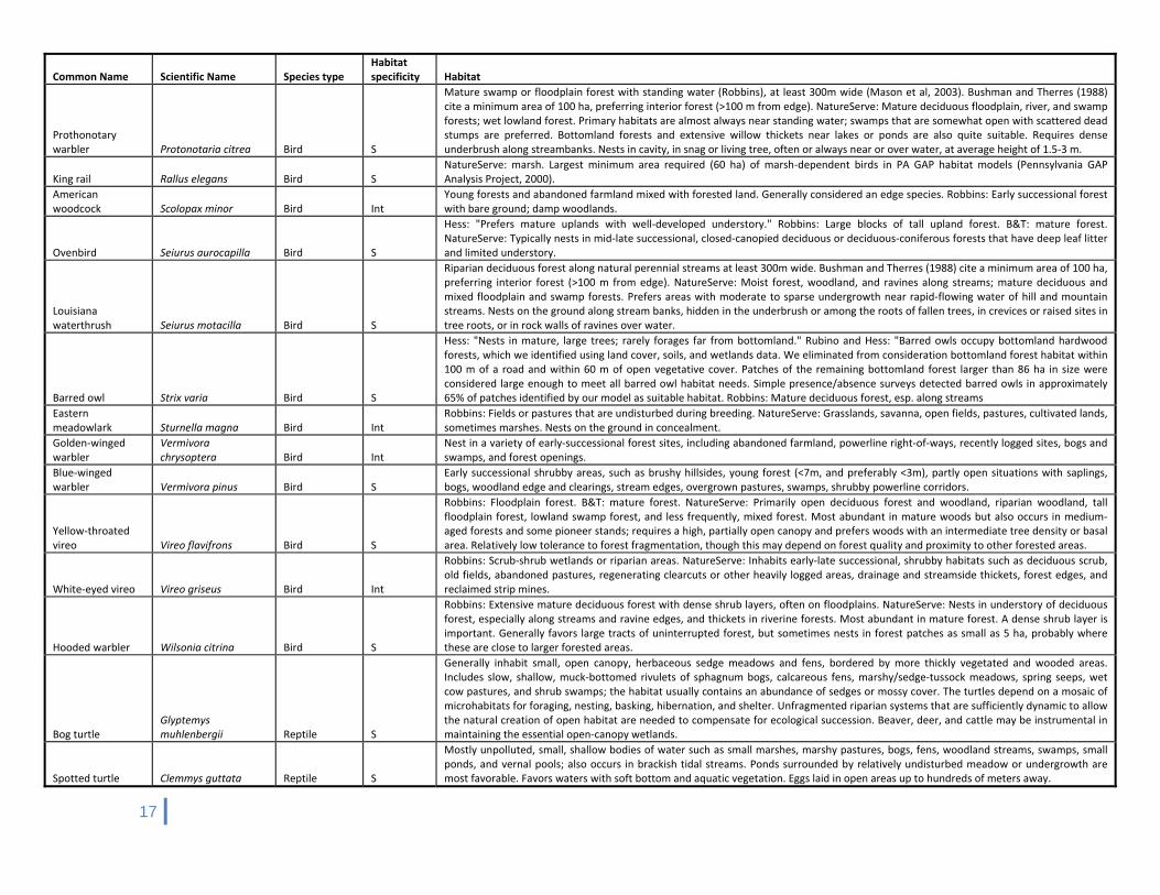
Prothonotary warbler Protonotaria citrea Bird S
Mature swamp or floodplain forest with standing water (Robbins), at least 300m wide (Mason et al, 2003). Bushman and Therres (1988) cite a minimum area of 100 ha, preferring interior forest (>100 m from edge). NatureServe: Mature deciduous floodplain, river, and swamp forests; wet lowland forest. Primary habitats are almost always near standing water; swamps that are somewhat open with scattered dead stumps are preferred. Bottomland forests and extensive willow thickets near lakes or ponds are also quite suitable. Requires dense underbrush along streambanks. Nests in cavity, in snag or living tree, often or always near or over water, at average height of 1.5‐3 m.
King rail Rallus elegans Bird S NatureServe: marsh. Largest minimum area required (60 ha) of marsh‐dependent birds in PA GAP habitat models (Pennsylvania GAP Analysis Project, 2000).
American woodcock Scolopax minor Bird Int
Young forests and abandoned farmland mixed with forested land. Generally considered an edge species. Robbins: Early successional forest with bare ground; damp woodlands.
Ovenbird Seiurus aurocapilla Bird S
Hess: "Prefers mature uplands with well‐developed understory." Robbins: Large blocks of tall upland forest. B&T: mature forest. NatureServe: Typically nests in mid‐late successional, closed‐canopied deciduous or deciduous‐coniferous forests that have deep leaf litter and limited understory.
Louisiana waterthrush Seiurus motacilla Bird S
Riparian deciduous forest along natural perennial streams at least 300m wide. Bushman and Therres (1988) cite a minimum area of 100 ha, preferring interior forest (>100 m from edge). NatureServe: Moist forest, woodland, and ravines along streams; mature deciduous and mixed floodplain and swamp forests. Prefers areas with moderate to sparse undergrowth near rapid‐flowing water of hill and mountain streams. Nests on the ground along stream banks, hidden in the underbrush or among the roots of fallen trees, in crevices or raised sites in tree roots, or in rock walls of ravines over water.
Barred owl Strix varia Bird S
Hess: "Nests in mature, large trees; rarely forages far from bottomland." Rubino and Hess: "Barred owls occupy bottomland hardwood forests, which we identified using land cover, soils, and wetlands data. We eliminated from consideration bottomland forest habitat within 100 m of a road and within 60 m of open vegetative cover. Patches of the remaining bottomland forest larger than 86 ha in size were considered large enough to meet all barred owl habitat needs. Simple presence/absence surveys detected barred owls in approximately 65% of patches identified by our model as suitable habitat. Robbins: Mature deciduous forest, esp. along streams
Eastern meadowlark Sturnella magna Bird Int
Robbins: Fields or pastures that are undisturbed during breeding. NatureServe: Grasslands, savanna, open fields, pastures, cultivated lands, sometimes marshes. Nests on the ground in concealment.
Golden‐winged warbler
Vermivora chrysoptera Bird Int
Nest in a variety of early‐successional forest sites, including abandoned farmland, powerline right‐of‐ways, recently logged sites, bogs and swamps, and forest openings.
Blue‐winged warbler Vermivora pinus Bird S
Early successional shrubby areas, such as brushy hillsides, young forest (<7m, and preferably <3m), partly open situations with saplings, bogs, woodland edge and clearings, stream edges, overgrown pastures, swamps, shrubby powerline corridors.
Yellow‐throated vireo Vireo flavifrons Bird S
Robbins: Floodplain forest. B&T: mature forest. NatureServe: Primarily open deciduous forest and woodland, riparian woodland, tall floodplain forest, lowland swamp forest, and less frequently, mixed forest. Most abundant in mature woods but also occurs in medium‐aged forests and some pioneer stands; requires a high, partially open canopy and prefers woods with an intermediate tree density or basal area. Relatively low tolerance to forest fragmentation, though this may depend on forest quality and proximity to other forested areas.
White‐eyed vireo Vireo griseus Bird Int
Robbins: Scrub‐shrub wetlands or riparian areas. NatureServe: Inhabits early‐late successional, shrubby habitats such as deciduous scrub, old fields, abandoned pastures, regenerating clearcuts or other heavily logged areas, drainage and streamside thickets, forest edges, and reclaimed strip mines.
Hooded warbler Wilsonia citrina Bird S
Robbins: Extensive mature deciduous forest with dense shrub layers, often on floodplains. NatureServe: Nests in understory of deciduous forest, especially along streams and ravine edges, and thickets in riverine forests. Most abundant in mature forest. A dense shrub layer is important. Generally favors large tracts of uninterrupted forest, but sometimes nests in forest patches as small as 5 ha, probably where these are close to larger forested areas.
Bog turtle Glyptemys muhlenbergii Reptile S
Generally inhabit small, open canopy, herbaceous sedge meadows and fens, bordered by more thickly vegetated and wooded areas. Includes slow, shallow, muck‐bottomed rivulets of sphagnum bogs, calcareous fens, marshy/sedge‐tussock meadows, spring seeps, wet cow pastures, and shrub swamps; the habitat usually contains an abundance of sedges or mossy cover. The turtles depend on a mosaic of microhabitats for foraging, nesting, basking, hibernation, and shelter. Unfragmented riparian systems that are sufficiently dynamic to allow the natural creation of open habitat are needed to compensate for ecological succession. Beaver, deer, and cattle may be instrumental in maintaining the essential open‐canopy wetlands.
Spotted turtle Clemmys guttata Reptile S
Mostly unpolluted, small, shallow bodies of water such as small marshes, marshy pastures, bogs, fens, woodland streams, swamps, small ponds, and vernal pools; also occurs in brackish tidal streams. Ponds surrounded by relatively undisturbed meadow or undergrowth are most favorable. Favors waters with soft bottom and aquatic vegetation. Eggs laid in open areas up to hundreds of meters away.
18
Common Name Scientific Name Species type Habitat specificity Habitat
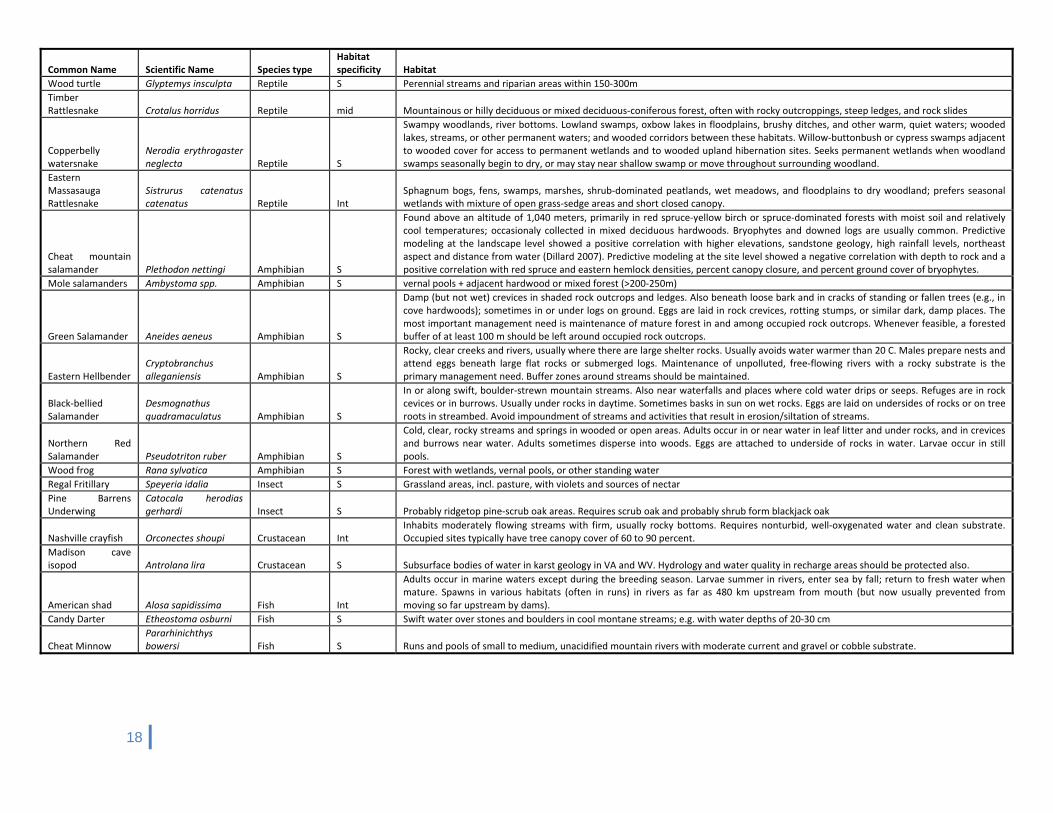
Wood turtle Glyptemys insculpta Reptile S Perennial streams and riparian areas within 150‐300m
Timber Rattlesnake Crotalus horridus Reptile mid Mountainous or hilly deciduous or mixed deciduous‐coniferous forest, often with rocky outcroppings, steep ledges, and rock slides
Copperbelly watersnake
Nerodia erythrogaster neglecta Reptile S
Swampy woodlands, river bottoms. Lowland swamps, oxbow lakes in floodplains, brushy ditches, and other warm, quiet waters; wooded lakes, streams, or other permanent waters; and wooded corridors between these habitats. Willow‐buttonbush or cypress swamps adjacent to wooded cover for access to permanent wetlands and to wooded upland hibernation sites. Seeks permanent wetlands when woodland swamps seasonally begin to dry, or may stay near shallow swamp or move throughout surrounding woodland.
Eastern Massasauga Rattlesnake
Sistrurus catenatus catenatus Reptile Int
Sphagnum bogs, fens, swamps, marshes, shrub‐dominated peatlands, wet meadows, and floodplains to dry woodland; prefers seasonal wetlands with mixture of open grass‐sedge areas and short closed canopy.
Cheat mountain salamander Plethodon nettingi Amphibian S
Found above an altitude of 1,040 meters, primarily in red spruce‐yellow birch or spruce‐dominated forests with moist soil and relatively cool temperatures; occasionaly collected in mixed deciduous hardwoods. Bryophytes and downed logs are usually common. Predictive modeling at the landscape level showed a positive correlation with higher elevations, sandstone geology, high rainfall levels, northeast aspect and distance from water (Dillard 2007). Predictive modeling at the site level showed a negative correlation with depth to rock and a positive correlation with red spruce and eastern hemlock densities, percent canopy closure, and percent ground cover of bryophytes.
Mole salamanders Ambystoma spp. Amphibian S vernal pools + adjacent hardwood or mixed forest (>200‐250m)
Green Salamander Aneides aeneus Amphibian S
Damp (but not wet) crevices in shaded rock outcrops and ledges. Also beneath loose bark and in cracks of standing or fallen trees (e.g., in cove hardwoods); sometimes in or under logs on ground. Eggs are laid in rock crevices, rotting stumps, or similar dark, damp places. The most important management need is maintenance of mature forest in and among occupied rock outcrops. Whenever feasible, a forested buffer of at least 100 m should be left around occupied rock outcrops.
Eastern Hellbender Cryptobranchus alleganiensis Amphibian S
Rocky, clear creeks and rivers, usually where there are large shelter rocks. Usually avoids water warmer than 20 C. Males prepare nests and attend eggs beneath large flat rocks or submerged logs. Maintenance of unpolluted, free‐flowing rivers with a rocky substrate is the primary management need. Buffer zones around streams should be maintained.
Black‐bellied Salamander
Desmognathus quadramaculatus Amphibian S
In or along swift, boulder‐strewn mountain streams. Also near waterfalls and places where cold water drips or seeps. Refuges are in rock cevices or in burrows. Usually under rocks in daytime. Sometimes basks in sun on wet rocks. Eggs are laid on undersides of rocks or on tree roots in streambed. Avoid impoundment of streams and activities that result in erosion/siltation of streams.
Northern Red Salamander Pseudotriton ruber Amphibian S
Cold, clear, rocky streams and springs in wooded or open areas. Adults occur in or near water in leaf litter and under rocks, and in crevices and burrows near water. Adults sometimes disperse into woods. Eggs are attached to underside of rocks in water. Larvae occur in still pools.
Wood frog Rana sylvatica Amphibian S Forest with wetlands, vernal pools, or other standing water
Regal Fritillary Speyeria idalia Insect S Grassland areas, incl. pasture, with violets and sources of nectar
Pine Barrens Underwing
Catocala herodias gerhardi Insect S Probably ridgetop pine‐scrub oak areas. Requires scrub oak and probably shrub form blackjack oak
Nashville crayfish Orconectes shoupi Crustacean Int Inhabits moderately flowing streams with firm, usually rocky bottoms. Requires nonturbid, well‐oxygenated water and clean substrate. Occupied sites typically have tree canopy cover of 60 to 90 percent.
Madison cave isopod Antrolana lira Crustacean S Subsurface bodies of water in karst geology in VA and WV. Hydrology and water quality in recharge areas should be protected also.
American shad Alosa sapidissima Fish Int
Adults occur in marine waters except during the breeding season. Larvae summer in rivers, enter sea by fall; return to fresh water when mature. Spawns in various habitats (often in runs) in rivers as far as 480 km upstream from mouth (but now usually prevented from moving so far upstream by dams).
Candy Darter Etheostoma osburni Fish S Swift water over stones and boulders in cool montane streams; e.g. with water depths of 20‐30 cm
Cheat Minnow Pararhinichthys bowersi Fish S Runs and pools of small to medium, unacidified mountain rivers with moderate current and gravel or cobble substrate.
19
Common Name Scientific Name Species type Habitat specificity Habitat
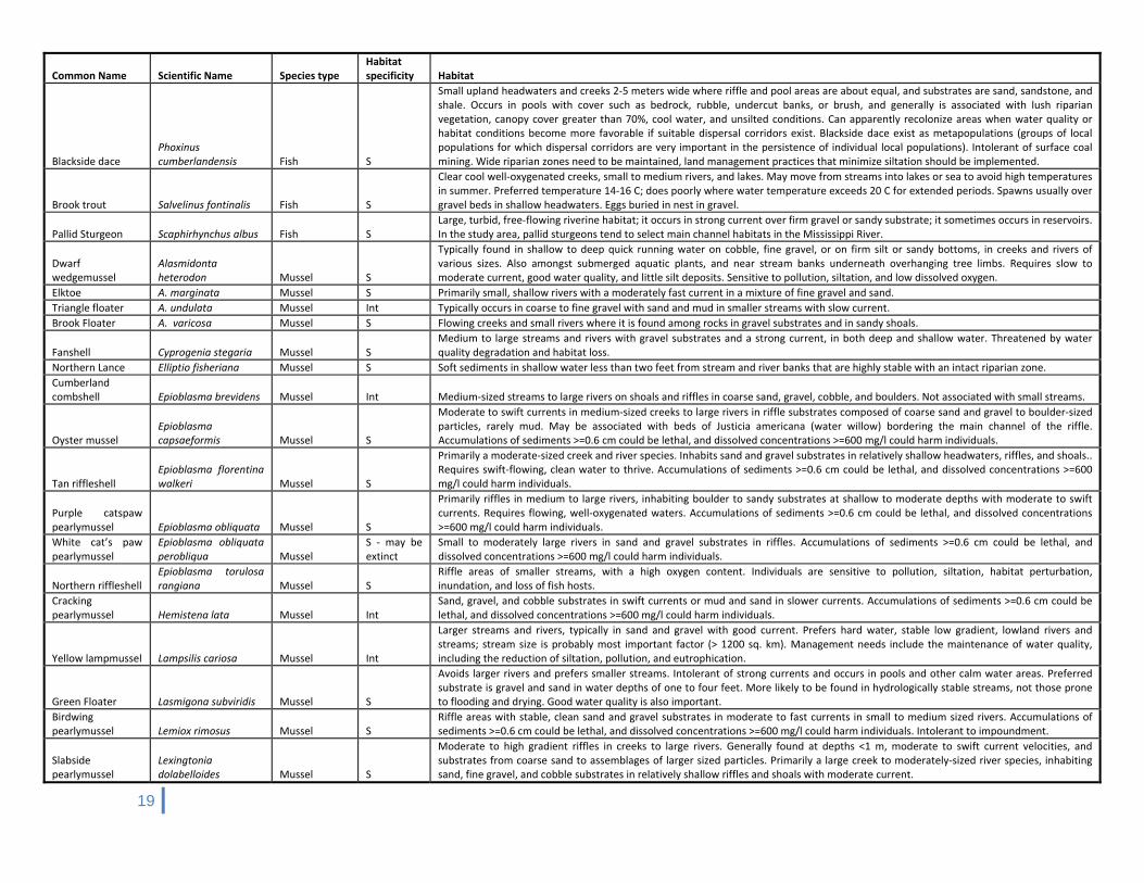
Blackside dace Phoxinus cumberlandensis Fish S
Small upland headwaters and creeks 2‐5 meters wide where riffle and pool areas are about equal, and substrates are sand, sandstone, and shale. Occurs in pools with cover such as bedrock, rubble, undercut banks, or brush, and generally is associated with lush riparian vegetation, canopy cover greater than 70%, cool water, and unsilted conditions. Can apparently recolonize areas when water quality or habitat conditions become more favorable if suitable dispersal corridors exist. Blackside dace exist as metapopulations (groups of local populations for which dispersal corridors are very important in the persistence of individual local populations). Intolerant of surface coal mining. Wide riparian zones need to be maintained, land management practices that minimize siltation should be implemented.
Brook trout Salvelinus fontinalis Fish S
Clear cool well‐oxygenated creeks, small to medium rivers, and lakes. May move from streams into lakes or sea to avoid high temperatures in summer. Preferred temperature 14‐16 C; does poorly where water temperature exceeds 20 C for extended periods. Spawns usually over gravel beds in shallow headwaters. Eggs buried in nest in gravel.
Pallid Sturgeon Scaphirhynchus albus Fish S Large, turbid, free‐flowing riverine habitat; it occurs in strong current over firm gravel or sandy substrate; it sometimes occurs in reservoirs. In the study area, pallid sturgeons tend to select main channel habitats in the Mississippi River.
Dwarf wedgemussel
Alasmidonta heterodon Mussel S
Typically found in shallow to deep quick running water on cobble, fine gravel, or on firm silt or sandy bottoms, in creeks and rivers of various sizes. Also amongst submerged aquatic plants, and near stream banks underneath overhanging tree limbs. Requires slow to moderate current, good water quality, and little silt deposits. Sensitive to pollution, siltation, and low dissolved oxygen.
Elktoe A. marginata Mussel S Primarily small, shallow rivers with a moderately fast current in a mixture of fine gravel and sand.
Triangle floater A. undulata Mussel Int Typically occurs in coarse to fine gravel with sand and mud in smaller streams with slow current.
Brook Floater A. varicosa Mussel S Flowing creeks and small rivers where it is found among rocks in gravel substrates and in sandy shoals.
Fanshell Cyprogenia stegaria Mussel S Medium to large streams and rivers with gravel substrates and a strong current, in both deep and shallow water. Threatened by water quality degradation and habitat loss.
Northern Lance Elliptio fisheriana Mussel S Soft sediments in shallow water less than two feet from stream and river banks that are highly stable with an intact riparian zone.
Cumberland combshell Epioblasma brevidens Mussel Int Medium‐sized streams to large rivers on shoals and riffles in coarse sand, gravel, cobble, and boulders. Not associated with small streams.
Oyster mussel Epioblasma capsaeformis Mussel S
Moderate to swift currents in medium‐sized creeks to large rivers in riffle substrates composed of coarse sand and gravel to boulder‐sized particles, rarely mud. May be associated with beds of Justicia americana (water willow) bordering the main channel of the riffle. Accumulations of sediments >=0.6 cm could be lethal, and dissolved concentrations >=600 mg/l could harm individuals.
Tan riffleshell Epioblasma florentina walkeri Mussel S
Primarily a moderate‐sized creek and river species. Inhabits sand and gravel substrates in relatively shallow headwaters, riffles, and shoals.. Requires swift‐flowing, clean water to thrive. Accumulations of sediments >=0.6 cm could be lethal, and dissolved concentrations >=600 mg/l could harm individuals.
Purple catspaw pearlymussel Epioblasma obliquata Mussel S
Primarily riffles in medium to large rivers, inhabiting boulder to sandy substrates at shallow to moderate depths with moderate to swift currents. Requires flowing, well‐oxygenated waters. Accumulations of sediments >=0.6 cm could be lethal, and dissolved concentrations >=600 mg/l could harm individuals.
White cat’s paw pearlymussel
Epioblasma obliquata perobliqua Mussel
S ‐ may be extinct
Small to moderately large rivers in sand and gravel substrates in riffles. Accumulations of sediments >=0.6 cm could be lethal, and dissolved concentrations >=600 mg/l could harm individuals.
Northern riffleshell Epioblasma torulosa rangiana Mussel S
Riffle areas of smaller streams, with a high oxygen content. Individuals are sensitive to pollution, siltation, habitat perturbation, inundation, and loss of fish hosts.
Cracking pearlymussel Hemistena lata Mussel Int
Sand, gravel, and cobble substrates in swift currents or mud and sand in slower currents. Accumulations of sediments >=0.6 cm could be lethal, and dissolved concentrations >=600 mg/l could harm individuals.
Yellow lampmussel Lampsilis cariosa Mussel Int
Larger streams and rivers, typically in sand and gravel with good current. Prefers hard water, stable low gradient, lowland rivers and streams; stream size is probably most important factor (> 1200 sq. km). Management needs include the maintenance of water quality, including the reduction of siltation, pollution, and eutrophication.
Green Floater Lasmigona subviridis Mussel S
Avoids larger rivers and prefers smaller streams. Intolerant of strong currents and occurs in pools and other calm water areas. Preferred substrate is gravel and sand in water depths of one to four feet. More likely to be found in hydrologically stable streams, not those prone to flooding and drying. Good water quality is also important.
Birdwing pearlymussel Lemiox rimosus Mussel S
Riffle areas with stable, clean sand and gravel substrates in moderate to fast currents in small to medium sized rivers. Accumulations of sediments >=0.6 cm could be lethal, and dissolved concentrations >=600 mg/l could harm individuals. Intolerant to impoundment.
Slabside pearlymussel
Lexingtonia dolabelloides Mussel S
Moderate to high gradient riffles in creeks to large rivers. Generally found at depths <1 m, moderate to swift current velocities, and substrates from coarse sand to assemblages of larger sized particles. Primarily a large creek to moderately‐sized river species, inhabiting sand, fine gravel, and cobble substrates in relatively shallow riffles and shoals with moderate current.
20
Common Name Scientific Name Species type Habitat specificity Habitat
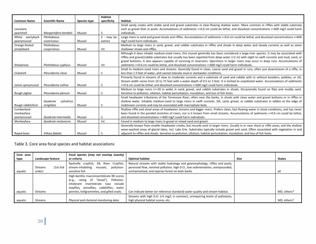
Louisiana pearlshell Margaritifera hembeli Mussel S
Small sandy creeks with stable sand and gravel substrates in clear‐flowing shallow water. More common in riffles with stable substrata such as gravel than in pools. Accumulations of sediments >=0.6 cm could be lethal, and dissolved concentrations >=600 mg/l could harm individuals.
White wartyback pearlymussel
Plethobasus cicatricosus Mussel
S ‐ may be extinct
Large rivers in sand and gravel shoals and riffles. Accumulations of sediments >=0.6 cm could be lethal, and dissolved concentrations >=600 mg/l could harm individuals.
Orange‐footed pimpleback
Plethobasus cooperianus Mussel Int
Medium to large rivers in sand, gravel, and cobble substrates in riffles and shoals in deep water and steady currents as well as some shallower shoals and riffles.
Sheepnose Plethobasus cyphyus Mussel Int
Although it does inhabit medium‐sized rivers, this mussel generally has been considered a large‐river species. It may be associated with riffles and gravel/cobble substrates but usually has been reported from deep water (>2 m) with slight to swift currents and mud, sand, or gravel bottoms. It also appears capable of surviving in reservoirs. Specimens in larger rivers may occur in deep runs. Accumulations of sediments >=0.6 cm could be lethal, and dissolved concentrations >=600 mg/l could harm individuals.
Clubshell Pleurobema clava Mussel S Small to medium‐sized rivers and streams. Generally found in clean, coarse sand and gravel in runs, often just downstream of a riffle, in less than 1.5 feet of water, and cannot tolerate mud or slackwater conditions.
James spinymussel Pleurobema collina Mussel S
Primarily found in streams of slow to moderate currents and a substrate of sand and cobble with or without boulders, pebbles, or silt. Stream width varies from 10 to 75 feet with a water depth of 0.5 to 3 feet. It is limited to unpolluted water. Accumulations of sediments >=0.6 cm could be lethal, and dissolved concentrations >=600 mg/l could harm individuals.
Rough pigtoe Pleurobema plenum Mussel S Medium to large rivers (>=20 m wide) in sand, gravel, and cobble substrates in shoals. Occasionally found on flats and muddy sand. Sensitive to pollution, siltation, habitat perturbation, inundation, and loss of fish hosts.
Rough rabbitsfoot Quadrula cylindrica strigillata Mussel S
Small headwater tributaries of the Tennessee River, often near the banks, in shoals with clean water and gravel bottoms or in riffles in shallow water. Inhabits medium‐sized to large rivers in swift currents. Silt, sand, gravel, or cobble substrates in eddies at the edge of midstream currents and may be associated with macrophyte beds.
Cumberland monkeyface pearlymussel Quadrula intermedia Mussel S
Shallow riffle and shoal areas of headwater streams and bigger rivers. Prefers clean, fast‐flowing water in shoal conditions, and has never been found in the ponded stretches of rivers, nor is it known from small streams. Accumulations of sediments >=0.6 cm could be lethal, and dissolved concentrations >=600 mg/l could harm individuals.
Monkeyface Quadrula metanevra Mussel Int Found in medium to large rivers in gravel or mixed sand and gravel.
Rayed bean Villosa fabalis Mussel S
Generally known from smaller headwater creeks, but records exist in larger rivers. Usually in or near shoal or riffle areas, and the shallow wave‐washed areas of glacial lakes, incl. Lake Erie. Substrates typically include gravel and sand. Often associated with vegetation in and adjacent to riffles and shoals. Sensitive to pollution, siltation, habitat perturbation, inundation, and loss of fish hosts.
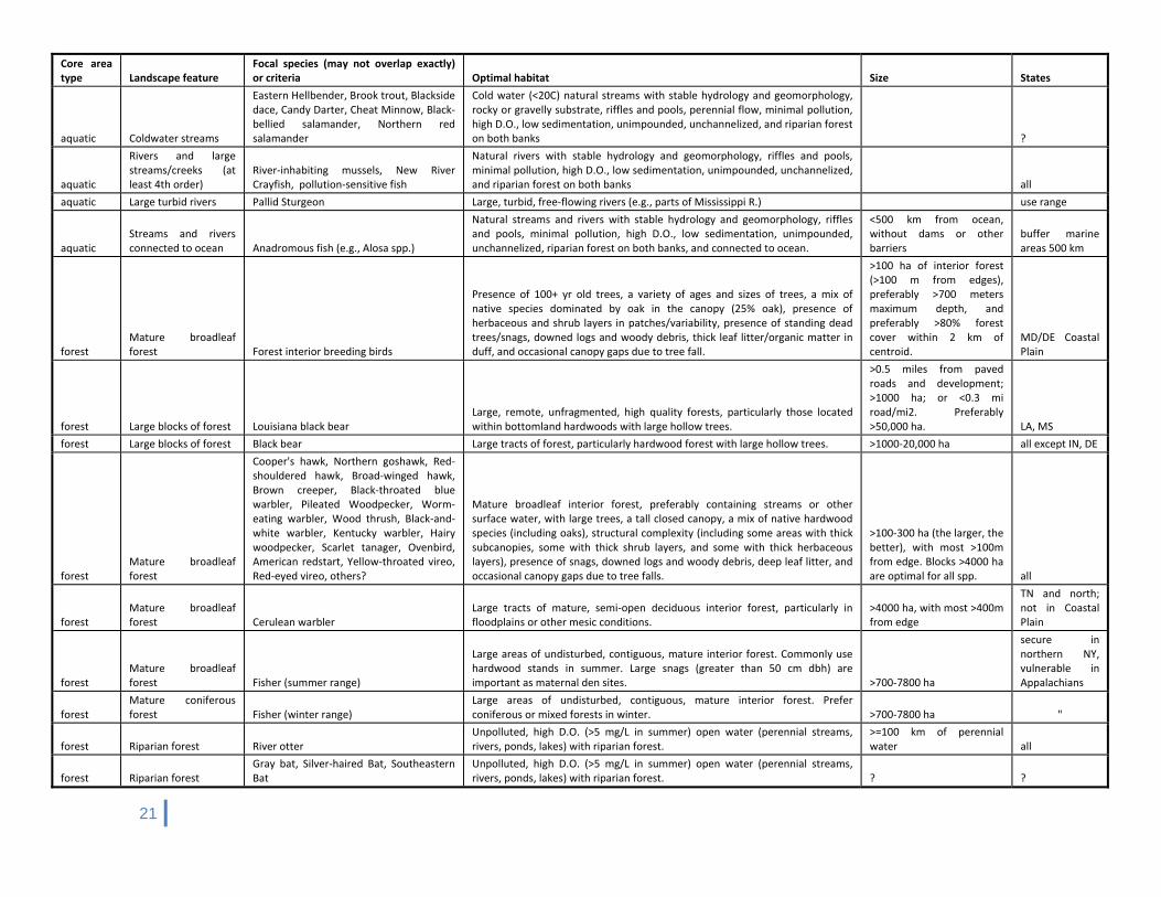
Table 3. Core area focal species and habitat associations Core area type Landscape feature
Focal species (may not overlap exactly) or criteria Optimal habitat Size States
aquatic Streams (1st‐3rd order)
Nashville crayfish, Elk River Crayfish, stream‐inhabiting mussels, pollution‐sensitive fish
Natural streams with stable hydrology and geomorphology, riffles and pools, perennial flow, minimal pollution, high D.O., low sedimentation, unimpounded, unchannelized, and riparian forest on both banks all
aquatic Streams
High benthic macroinvertebrate IBI scores (e.g., rating of "Good"). Pollution‐intolerant invertebrate taxa include mayflies, stoneflies, caddisflies, water pennies, hellgrammites, and gilled snails. Can indicate better (or reference standard) water quality and stream habitat. MD, others?
aquatic Streams Physical and chemical monitoring data Streams with high D.O. (>5 mg/L in summer), unimpairing levels of pollutants, high physical habitat scores, etc. MD, others?
21
Core area type Landscape feature
Focal species (may not overlap exactly) or criteria Optimal habitat Size States
aquatic Coldwater streams
Eastern Hellbender, Brook trout, Blackside dace, Candy Darter, Cheat Minnow, Black‐bellied salamander, Northern red salamander
Cold water (<20C) natural streams with stable hydrology and geomorphology, rocky or gravelly substrate, riffles and pools, perennial flow, minimal pollution, high D.O., low sedimentation, unimpounded, unchannelized, and riparian forest on both banks ?
aquatic
Rivers and large streams/creeks (at least 4th order)
River‐inhabiting mussels, New River Crayfish, pollution‐sensitive fish
Natural rivers with stable hydrology and geomorphology, riffles and pools, minimal pollution, high D.O., low sedimentation, unimpounded, unchannelized, and riparian forest on both banks all
aquatic Large turbid rivers Pallid Sturgeon Large, turbid, free‐flowing rivers (e.g., parts of Mississippi R.) use range
aquatic Streams and rivers connected to ocean Anadromous fish (e.g., Alosa spp.)
Natural streams and rivers with stable hydrology and geomorphology, riffles and pools, minimal pollution, high D.O., low sedimentation, unimpounded, unchannelized, riparian forest on both banks, and connected to ocean.
<500 km from ocean, without dams or other barriers
buffer marine areas 500 km
forest Mature broadleaf forest Forest interior breeding birds
Presence of 100+ yr old trees, a variety of ages and sizes of trees, a mix of native species dominated by oak in the canopy (25% oak), presence of herbaceous and shrub layers in patches/variability, presence of standing dead trees/snags, downed logs and woody debris, thick leaf litter/organic matter in duff, and occasional canopy gaps due to tree fall.
>100 ha of interior forest (>100 m from edges), preferably >700 meters maximum depth, and preferably >80% forest cover within 2 km of centroid.
MD/DE Coastal Plain
forest Large blocks of forest Louisiana black bear Large, remote, unfragmented, high quality forests, particularly those located within bottomland hardwoods with large hollow trees.
>0.5 miles from paved roads and development; >1000 ha; or <0.3 mi road/mi2. Preferably >50,000 ha. LA, MS
forest Large blocks of forest Black bear Large tracts of forest, particularly hardwood forest with large hollow trees. >1000‐20,000 ha all except IN, DE
forest Mature broadleaf forest
Cooper's hawk, Northern goshawk, Red‐shouldered hawk, Broad‐winged hawk, Brown creeper, Black‐throated blue warbler, Pileated Woodpecker, Worm‐eating warbler, Wood thrush, Black‐and‐white warbler, Kentucky warbler, Hairy woodpecker, Scarlet tanager, Ovenbird, American redstart, Yellow‐throated vireo, Red‐eyed vireo, others?
Mature broadleaf interior forest, preferably containing streams or other surface water, with large trees, a tall closed canopy, a mix of native hardwood species (including oaks), structural complexity (including some areas with thick subcanopies, some with thick shrub layers, and some with thick herbaceous layers), presence of snags, downed logs and woody debris, deep leaf litter, and occasional canopy gaps due to tree falls.
>100‐300 ha (the larger, the better), with most >100m from edge. Blocks >4000 ha are optimal for all spp. all
forest Mature broadleaf forest Cerulean warbler
Large tracts of mature, semi‐open deciduous interior forest, particularly in floodplains or other mesic conditions.
>4000 ha, with most >400m from edge
TN and north; not in Coastal Plain
forest Mature broadleaf forest Fisher (summer range)
Large areas of undisturbed, contiguous, mature interior forest. Commonly use hardwood stands in summer. Large snags (greater than 50 cm dbh) are important as maternal den sites. >700‐7800 ha
secure in northern NY, vulnerable in Appalachians
forest Mature coniferous forest Fisher (winter range)
Large areas of undisturbed, contiguous, mature interior forest. Prefer coniferous or mixed forests in winter. >700‐7800 ha "
forest Riparian forest River otter Unpolluted, high D.O. (>5 mg/L in summer) open water (perennial streams, rivers, ponds, lakes) with riparian forest.
>=100 km of perennial water all
forest Riparian forest Gray bat, Silver‐haired Bat, Southeastern Bat
Unpolluted, high D.O. (>5 mg/L in summer) open water (perennial streams, rivers, ponds, lakes) with riparian forest. ? ?
22
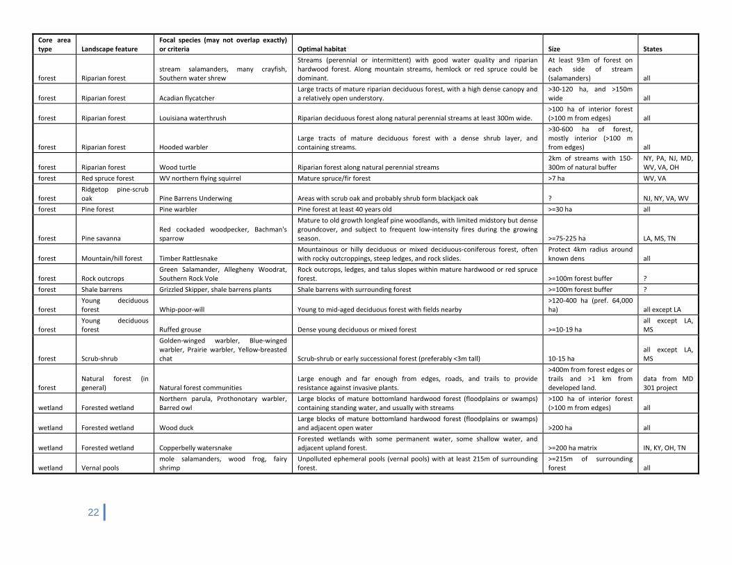
Core area type Landscape feature
Focal species (may not overlap exactly) or criteria Optimal habitat Size States
forest Riparian forest stream salamanders, many crayfish, Southern water shrew
Streams (perennial or intermittent) with good water quality and riparian hardwood forest. Along mountain streams, hemlock or red spruce could be dominant.
At least 93m of forest on each side of stream (salamanders) all
forest Riparian forest Acadian flycatcher Large tracts of mature riparian deciduous forest, with a high dense canopy and a relatively open understory.
>30‐120 ha, and >150m wide all
forest Riparian forest Louisiana waterthrush Riparian deciduous forest along natural perennial streams at least 300m wide. >100 ha of interior forest (>100 m from edges) all
forest Riparian forest Hooded warbler Large tracts of mature deciduous forest with a dense shrub layer, and containing streams.
>30‐600 ha of forest, mostly interior (>100 m from edges) all
forest Riparian forest Wood turtle Riparian forest along natural perennial streams 2km of streams with 150‐300m of natural buffer
NY, PA, NJ, MD, WV, VA, OH
forest Red spruce forest WV northern flying squirrel Mature spruce/fir forest >7 ha WV, VA
forest Ridgetop pine‐scrub oak Pine Barrens Underwing Areas with scrub oak and probably shrub form blackjack oak ? NJ, NY, VA, WV
forest Pine forest Pine warbler Pine forest at least 40 years old >=30 ha all
forest Pine savanna Red cockaded woodpecker, Bachman's sparrow
Mature to old growth longleaf pine woodlands, with limited midstory but dense groundcover, and subject to frequent low‐intensity fires during the growing season. >=75‐225 ha LA, MS, TN
forest Mountain/hill forest Timber Rattlesnake Mountainous or hilly deciduous or mixed deciduous‐coniferous forest, often with rocky outcroppings, steep ledges, and rock slides.
Protect 4km radius around known dens all
forest Rock outcrops Green Salamander, Allegheny Woodrat, Southern Rock Vole
Rock outcrops, ledges, and talus slopes within mature hardwood or red spruce forest. >=100m forest buffer ?
forest Shale barrens Grizzled Skipper, shale barrens plants Shale barrens with surrounding forest >=100m forest buffer ?
forest Young deciduous forest Whip‐poor‐will Young to mid‐aged deciduous forest with fields nearby
>120‐400 ha (pref. 64,000 ha) all except LA
forest Young deciduous forest Ruffed grouse Dense young deciduous or mixed forest >=10‐19 ha
all except LA, MS
forest Scrub‐shrub
Golden‐winged warbler, Blue‐winged warbler, Prairie warbler, Yellow‐breasted chat Scrub‐shrub or early successional forest (preferably <3m tall) 10‐15 ha
all except LA, MS
forest Natural forest (in general) Natural forest communities
Large enough and far enough from edges, roads, and trails to provide resistance against invasive plants.
>400m from forest edges or trails and >1 km from developed land.
data from MD 301 project
wetland Forested wetland Northern parula, Prothonotary warbler, Barred owl
Large blocks of mature bottomland hardwood forest (floodplains or swamps) containing standing water, and usually with streams
>100 ha of interior forest (>100 m from edges) all
wetland Forested wetland Wood duck Large blocks of mature bottomland hardwood forest (floodplains or swamps) and adjacent open water >200 ha all
wetland Forested wetland Copperbelly watersnake Forested wetlands with some permanent water, some shallow water, and adjacent upland forest. >=200 ha matrix IN, KY, OH, TN
wetland Vernal pools mole salamanders, wood frog, fairy shrimp
Unpolluted ephemeral pools (vernal pools) with at least 215m of surrounding forest.
>=215m of surrounding forest all
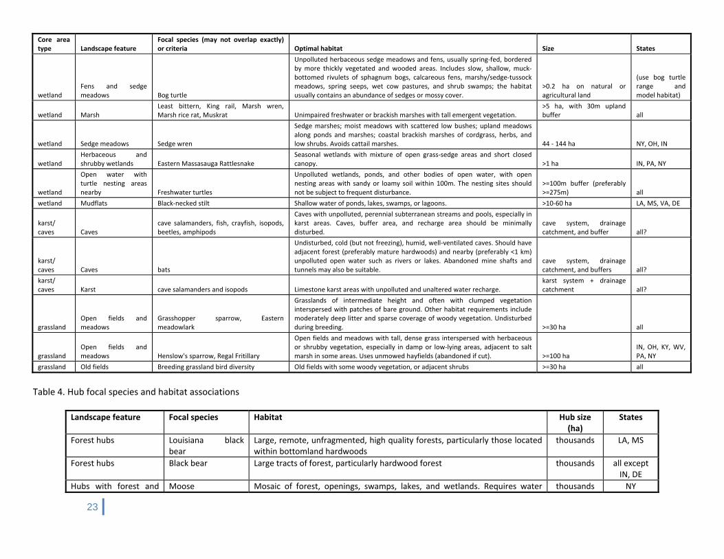
23
Core area type Landscape feature
Focal species (may not overlap exactly) or criteria Optimal habitat Size States
wetland Fens and sedge meadows Bog turtle
Unpolluted herbaceous sedge meadows and fens, usually spring‐fed, bordered by more thickly vegetated and wooded areas. Includes slow, shallow, muck‐bottomed rivulets of sphagnum bogs, calcareous fens, marshy/sedge‐tussock meadows, spring seeps, wet cow pastures, and shrub swamps; the habitat usually contains an abundance of sedges or mossy cover.
>0.2 ha on natural or agricultural land
(use bog turtle range and model habitat)
wetland Marsh Least bittern, King rail, Marsh wren, Marsh rice rat, Muskrat Unimpaired freshwater or brackish marshes with tall emergent vegetation.
>5 ha, with 30m upland buffer all
wetland Sedge meadows Sedge wren
Sedge marshes; moist meadows with scattered low bushes; upland meadows along ponds and marshes; coastal brackish marshes of cordgrass, herbs, and low shrubs. Avoids cattail marshes. 44 ‐ 144 ha NY, OH, IN
wetland Herbaceous and shrubby wetlands Eastern Massasauga Rattlesnake
Seasonal wetlands with mixture of open grass‐sedge areas and short closed canopy. >1 ha IN, PA, NY
wetland
Open water with turtle nesting areas nearby Freshwater turtles
Unpolluted wetlands, ponds, and other bodies of open water, with open nesting areas with sandy or loamy soil within 100m. The nesting sites should not be subject to frequent disturbance.
>=100m buffer (preferably >=275m) all
wetland Mudflats Black‐necked stilt Shallow water of ponds, lakes, swamps, or lagoons. >10‐60 ha LA, MS, VA, DE
karst/ caves Caves
cave salamanders, fish, crayfish, isopods, beetles, amphipods
Caves with unpolluted, perennial subterranean streams and pools, especially in karst areas. Caves, buffer area, and recharge area should be minimally disturbed.
cave system, drainage catchment, and buffer all?
karst/ caves Caves bats
Undisturbed, cold (but not freezing), humid, well‐ventilated caves. Should have adjacent forest (preferably mature hardwoods) and nearby (preferably <1 km) unpolluted open water such as rivers or lakes. Abandoned mine shafts and tunnels may also be suitable.
cave system, drainage catchment, and buffers all?
karst/ caves Karst cave salamanders and isopods Limestone karst areas with unpolluted and unaltered water recharge.
karst system + drainage catchment all?
grassland Open fields and meadows
Grasshopper sparrow, Eastern meadowlark
Grasslands of intermediate height and often with clumped vegetation interspersed with patches of bare ground. Other habitat requirements include moderately deep litter and sparse coverage of woody vegetation. Undisturbed during breeding. >=30 ha all
grassland Open fields and meadows Henslow's sparrow, Regal Fritillary
Open fields and meadows with tall, dense grass interspersed with herbaceous or shrubby vegetation, especially in damp or low‐lying areas, adjacent to salt marsh in some areas. Uses unmowed hayfields (abandoned if cut). >=100 ha
IN, OH, KY, WV, PA, NY
grassland Old fields Breeding grassland bird diversity Old fields with some woody vegetation, or adjacent shrubs >=30 ha all
Table 4. Hub focal species and habitat associations
Landscape feature Focal species Habitat Hub size (ha)
States
Forest hubs Louisiana black bear
Large, remote, unfragmented, high quality forests, particularly those located within bottomland hardwoods
thousands LA, MS
Forest hubs Black bear Large tracts of forest, particularly hardwood forest thousands all except IN, DE
Hubs with forest and Moose Mosaic of forest, openings, swamps, lakes, and wetlands. Requires water thousands NY
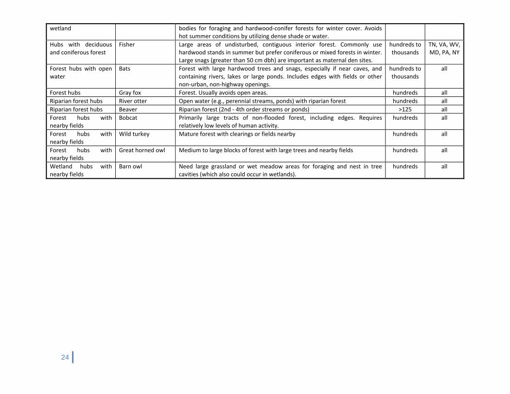
24
wetland bodies for foraging and hardwood‐conifer forests for winter cover. Avoids hot summer conditions by utilizing dense shade or water.
Hubs with deciduous and coniferous forest
Fisher Large areas of undisturbed, contiguous interior forest. Commonly use hardwood stands in summer but prefer coniferous or mixed forests in winter. Large snags (greater than 50 cm dbh) are important as maternal den sites.
hundreds to thousands
TN, VA, WV, MD, PA, NY
Forest hubs with open water
Bats Forest with large hardwood trees and snags, especially if near caves, and containing rivers, lakes or large ponds. Includes edges with fields or other non‐urban, non‐highway openings.
hundreds to thousands
all
Forest hubs Gray fox Forest. Usually avoids open areas. hundreds all
Riparian forest hubs River otter Open water (e.g., perennial streams, ponds) with riparian forest hundreds all
Riparian forest hubs Beaver Riparian forest (2nd ‐ 4th order streams or ponds) >125 all
Forest hubs with nearby fields
Bobcat Primarily large tracts of non‐flooded forest, including edges. Requires relatively low levels of human activity.
hundreds all
Forest hubs with nearby fields
Wild turkey Mature forest with clearings or fields nearby hundreds all
Forest hubs with nearby fields
Great horned owl Medium to large blocks of forest with large trees and nearby fields hundreds all
Wetland hubs with nearby fields
Barn owl Need large grassland or wet meadow areas for foraging and nest in tree cavities (which also could occur in wetlands).
hundreds all
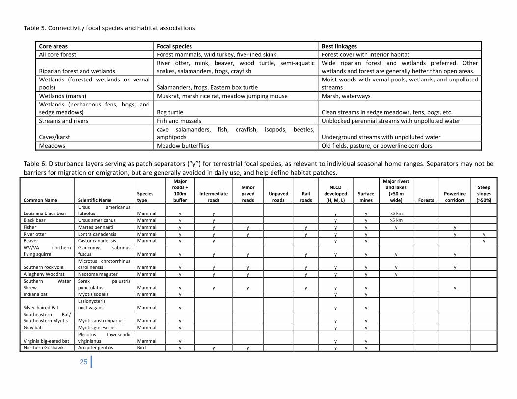
25
Table 5. Connectivity focal species and habitat associations
Core areas Focal species Best linkages
All core forest Forest mammals, wild turkey, five‐lined skink Forest cover with interior habitat
Riparian forest and wetlands River otter, mink, beaver, wood turtle, semi‐aquatic snakes, salamanders, frogs, crayfish
Wide riparian forest and wetlands preferred. Other wetlands and forest are generally better than open areas.
Wetlands (forested wetlands or vernal pools) Salamanders, frogs, Eastern box turtle
Moist woods with vernal pools, wetlands, and unpolluted streams
Wetlands (marsh) Muskrat, marsh rice rat, meadow jumping mouse Marsh, waterways
Wetlands (herbaceous fens, bogs, and sedge meadows) Bog turtle Clean streams in sedge meadows, fens, bogs, etc.
Streams and rivers Fish and mussels Unblocked perennial streams with unpolluted water
Caves/karst cave salamanders, fish, crayfish, isopods, beetles, amphipods Underground streams with unpolluted water
Meadows Meadow butterflies Old fields, pasture, or powerline corridors
Table 6. Disturbance layers serving as patch separators (“y”) for terrestrial focal species, as relevant to individual seasonal home ranges. Separators may not be barriers for migration or emigration, but are generally avoided in daily use, and help define habitat patches.
Common Name Scientific Name Species type
Major roads + 100m buffer
Intermediate roads
Minor paved roads
Unpaved roads
Rail roads
NLCD developed (H, M, L)
Surface mines
Major rivers and lakes (>50 m wide) Forests
Powerline corridors
Steep slopes (>50%)
Louisiana black bear Ursus americanus luteolus Mammal y y y y >5 km
Black bear Ursus americanus Mammal y y y y >5 km
Fisher Martes pennanti Mammal y y y y y y y y
River otter Lontra canadensis Mammal y y y y y y y y
Beaver Castor canadensis Mammal y y y y y
WV/VA northern flying squirrel
Glaucomys sabrinus fuscus Mammal y y y y y y y y
Southern rock vole Microtus chrotorrhinus carolinensis Mammal y y y y y y y y
Allegheny Woodrat Neotoma magister Mammal y y y y y y y
Southern Water Shrew
Sorex palustris punctulatus Mammal y y y y y y y
Indiana bat Myotis sodalis Mammal y y y
Silver‐haired Bat Lasionycteris noctivagans Mammal y y y
Southeastern Bat/ Southeastern Myotis Myotis austroriparius Mammal y y y
Gray bat Myotis grisescens Mammal y y y
Virginia big‐eared bat Plecotus townsendii virginianus Mammal y y y
Northern Goshawk Accipiter gentilis Bird y y y y y
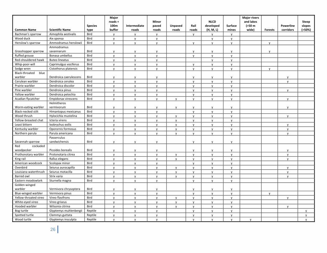
26
Common Name Scientific Name Species type
Major roads + 100m buffer
Intermediate roads
Minor paved roads
Unpaved roads
Rail roads
NLCD developed (H, M, L)
Surface mines
Major rivers and lakes (>50 m wide) Forests
Powerline corridors
Steep slopes (>50%)
Bachman's sparrow Aimophila aestivalis Bird y y y y y y
Wood duck Aix sponsa Bird y y y y y
Henslow's sparrow Ammodramus henslowii Bird y y y y y y y
Grasshopper sparrow Ammodramus savannarum Bird y y y y y y y
Ruffed grouse Bonasa umbellus Bird y y y y y y
Red‐shouldered hawk Buteo lineatus Bird y y y y y
Whip‐poor‐will Caprimulgus vociferus Bird y y y y y y
Sedge wren Cistothorus platensis Bird y y y y y y y
Black‐throated blue warbler Dendroica caerulescens Bird y y y y y y y
Cerulean warbler Dendroica cerulea Bird y y y y y y y
Prairie warbler Dendroica discolor Bird y y y y y y
Pine warbler Dendroica pinus Bird y y y y y y y
Yellow warbler Dendroica petechia Bird y y y y y y
Acadian flycatcher Empidonax virescens Bird y y y y y y y y
Worm‐eating warbler Helmitheros vermivorum Bird y y y y y y y y
Black‐necked stilt Himantopus mexicanus Bird y y y y y y
Wood thrush Hylocichla mustelina Bird y y y y y y y y
Yellow‐breasted chat Icteria virens Bird y y y y y y y
Least bittern Ixobrychus exilis Bird y y y y y y y y
Kentucky warbler Oporornis formosus Bird y y y y y y y y
Northern parula Parula americana Bird y y y y y y y y
Savannah sparrow Passerculus sandwichensis Bird y y y y y y
Red cockaded woodpecker Picoides borealis Bird y y y y y y y
Prothonotary warbler Protonotaria citrea Bird y y y y y y y y
King rail Rallus elegans Bird y y y y y y y y
American woodcock Scolopax minor Bird y y y y y y
Ovenbird Seiurus aurocapilla Bird y y y y y y y y
Louisiana waterthrush Seiurus motacilla Bird y y y y y y y y
Barred owl Strix varia Bird y y y y y y y y
Eastern meadowlark Sturnella magna Bird y y y y y y
Golden‐winged warbler Vermivora chrysoptera Bird y y y y y y
Blue‐winged warbler Vermivora pinus Bird y y y y y y y
Yellow‐throated vireo Vireo flavifrons Bird y y y y y y y y
White‐eyed vireo Vireo griseus Bird y y y y y y y
Hooded warbler Wilsonia citrina Bird y y y y y y y y
Bog turtle Glyptemys muhlenbergii Reptile y y y y y y y
Spotted turtle Clemmys guttata Reptile y y y y y y y
Wood turtle Glyptemys insculpta Reptile y y y y y y y y
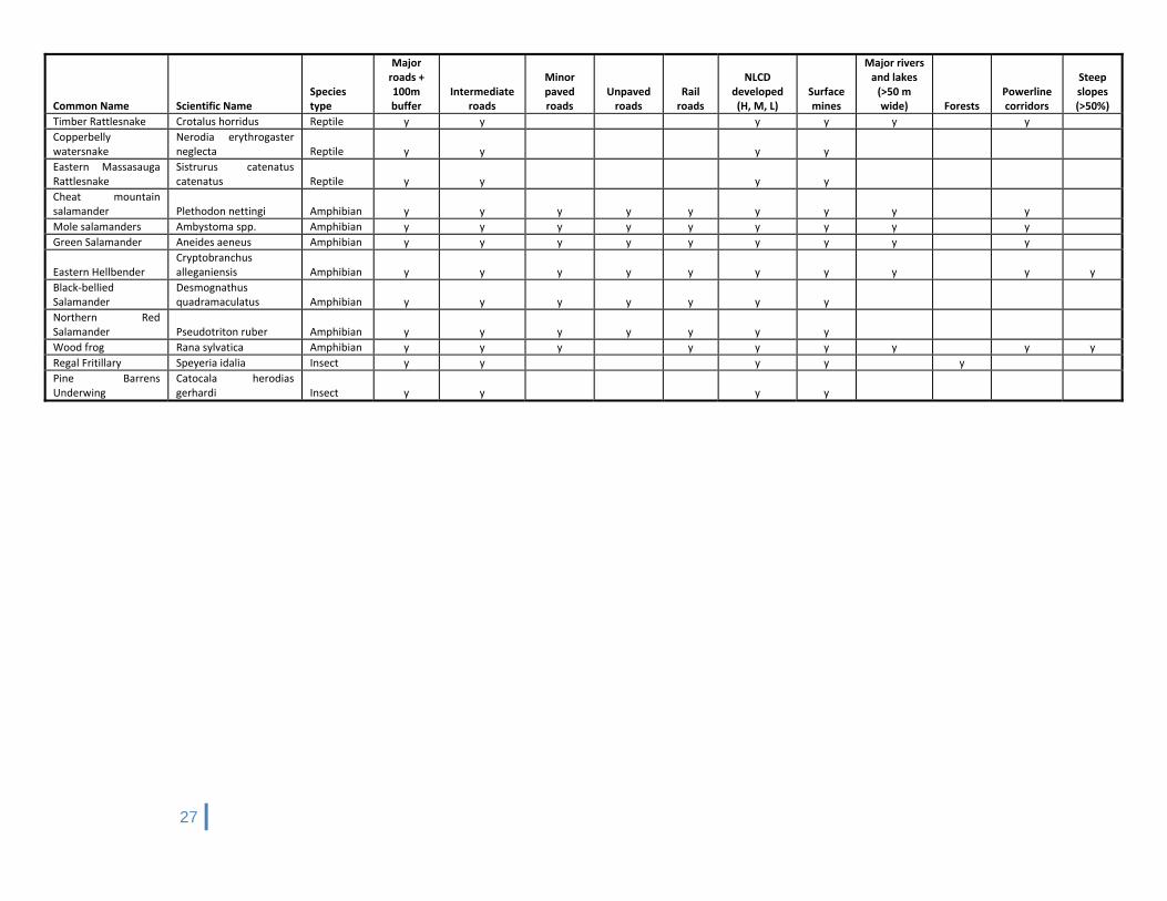
27
Common Name Scientific Name Species type
Major roads + 100m buffer
Intermediate roads
Minor paved roads
Unpaved roads
Rail roads
NLCD developed (H, M, L)
Surface mines
Major rivers and lakes (>50 m wide) Forests
Powerline corridors
Steep slopes (>50%)
Timber Rattlesnake Crotalus horridus Reptile y y y y y y
Copperbelly watersnake
Nerodia erythrogaster neglecta Reptile y y y y
Eastern Massasauga Rattlesnake
Sistrurus catenatus catenatus Reptile y y y y
Cheat mountain salamander Plethodon nettingi Amphibian y y y y y y y y y
Mole salamanders Ambystoma spp. Amphibian y y y y y y y y y
Green Salamander Aneides aeneus Amphibian y y y y y y y y y
Eastern Hellbender Cryptobranchus alleganiensis Amphibian y y y y y y y y y y
Black‐bellied Salamander
Desmognathus quadramaculatus Amphibian y y y y y y y
Northern Red Salamander Pseudotriton ruber Amphibian y y y y y y y
Wood frog Rana sylvatica Amphibian y y y y y y y y y
Regal Fritillary Speyeria idalia Insect y y y y y
Pine Barrens Underwing
Catocala herodias gerhardi Insect y y y y
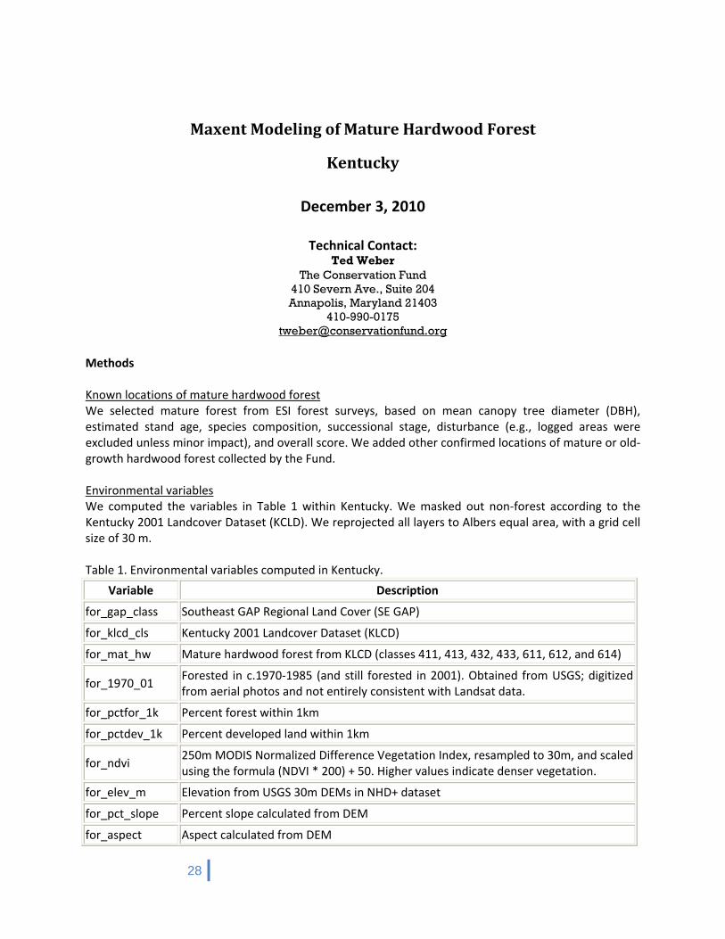
28
Maxent Modeling of Mature Hardwood Forest
Kentucky
December 3, 2010
Technical Contact: Ted Weber
The Conservation Fund 410 Severn Ave., Suite 204 Annapolis, Maryland 21403
410-990-0175 [email protected]
Methods Known locations of mature hardwood forest We selected mature forest from ESI forest surveys, based on mean canopy tree diameter (DBH), estimated stand age, species composition, successional stage, disturbance (e.g., logged areas were excluded unless minor impact), and overall score. We added other confirmed locations of mature or old‐growth hardwood forest collected by the Fund. Environmental variables We computed the variables in Table 1 within Kentucky. We masked out non‐forest according to the Kentucky 2001 Landcover Dataset (KCLD). We reprojected all layers to Albers equal area, with a grid cell size of 30 m. Table 1. Environmental variables computed in Kentucky.
Variable Description
for_gap_class Southeast GAP Regional Land Cover (SE GAP)
for_klcd_cls Kentucky 2001 Landcover Dataset (KLCD)
for_mat_hw Mature hardwood forest from KLCD (classes 411, 413, 432, 433, 611, 612, and 614)
for_1970_01 Forested in c.1970‐1985 (and still forested in 2001). Obtained from USGS; digitized from aerial photos and not entirely consistent with Landsat data.
for_pctfor_1k Percent forest within 1km
for_pctdev_1k Percent developed land within 1km
for_ndvi 250m MODIS Normalized Difference Vegetation Index, resampled to 30m, and scaled using the formula (NDVI * 200) + 50. Higher values indicate denser vegetation.
for_elev_m Elevation from USGS 30m DEMs in NHD+ dataset
for_pct_slope Percent slope calculated from DEM
for_aspect Aspect calculated from DEM

29
for_lg_tpi Topographic position index calculated in a 2010 m radius
for_sm_tpi Topographic position index calculated in a 510 m radius
for_landform Landform classification
for_max_temp7 Maximum July temperature (C x 10) from ClimateSource (1971‐2000 average; ~400 m resolution)
for_min_temp7 Minimum July temperature (C x 10) from ClimateSource (1971‐2000 average; ~400 m resolution)
for_meantemp7 Mean July temperature (C x 10) from ClimateSource (1971‐2000 average; ~400 m resolution)
for_precip_7 Mean July rainfall (mm) from ClimateSource (1971‐2000 average; ~400 m resolution)
for_solar_ins June insolation, calculated from 30m DEMs and latitude
for_dist_strm Distance to nearest stream (m)
Maxent model We used 10‐fold cross‐validation, which split the sample into ten different sets of 51‐52 training samples and 5‐6 test samples. We set parameters as follows:
Output format = logistic
Use all possible variable relationships (linear, quadratic, product, threshold, and hinge)
Regularization multiplier = 1
Maximum number of background points = 10,000
Crossvalidate with 10 replicates
Add samples to background
Extrapolate
Do clamping
Maximum number of iterations = 500
Convergence threshold = 0.00001 We also ran Maxent with the same data and parameters, except with automatically selected variable relationships based on the number of sample points. Spatial application We converted Maxent ASCII output to a floating point grid:
Arc: asciigrid mature_hardwood_forest_avg.asc flt_mat_hw float We multiplied this by 100 and took the integer value:
Grid: mature_hw_avg = int(flt_mat_hw * 100) We selected the Maxent threshold that captured the highest proportion of test points, while covering the least area of forest. Generally, this corresponds to the maximum test sensitivity plus specificity. We only considered thresholds with p<0.05. We reclassified the Maxent grid to a binary format (1 = above the threshold; 0 = below), and smoothed this by removing isolated areas <1 ac and filling holes <1 ac. We converted the resultant grid (KY_mature_hw) to a shapefile (KY_mature_hardwood_forest_from_Maxent.shp). Results
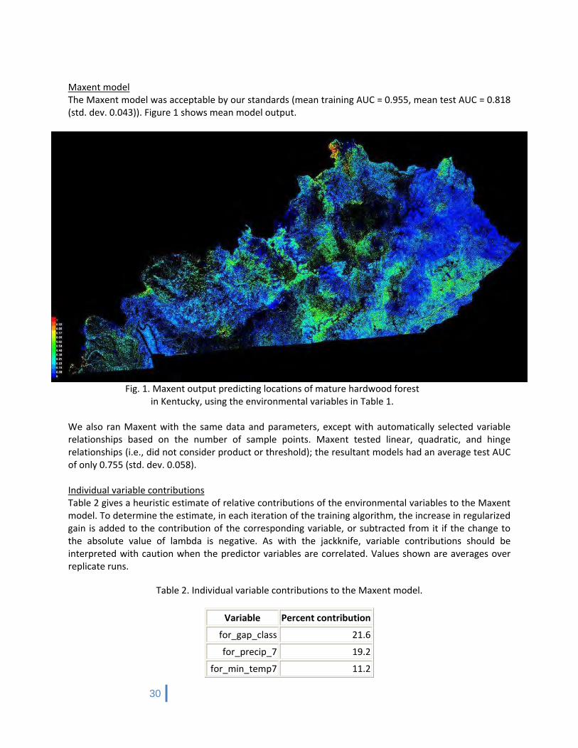
30
Maxent model The Maxent model was acceptable by our standards (mean training AUC = 0.955, mean test AUC = 0.818 (std. dev. 0.043)). Figure 1 shows mean model output.
Fig. 1. Maxent output predicting locations of mature hardwood forest in Kentucky, using the environmental variables in Table 1.
We also ran Maxent with the same data and parameters, except with automatically selected variable relationships based on the number of sample points. Maxent tested linear, quadratic, and hinge relationships (i.e., did not consider product or threshold); the resultant models had an average test AUC of only 0.755 (std. dev. 0.058). Individual variable contributions Table 2 gives a heuristic estimate of relative contributions of the environmental variables to the Maxent model. To determine the estimate, in each iteration of the training algorithm, the increase in regularized gain is added to the contribution of the corresponding variable, or subtracted from it if the change to the absolute value of lambda is negative. As with the jackknife, variable contributions should be interpreted with caution when the predictor variables are correlated. Values shown are averages over replicate runs.
Table 2. Individual variable contributions to the Maxent model.
Variable Percent contribution
for_gap_class 21.6
for_precip_7 19.2
for_min_temp7 11.2
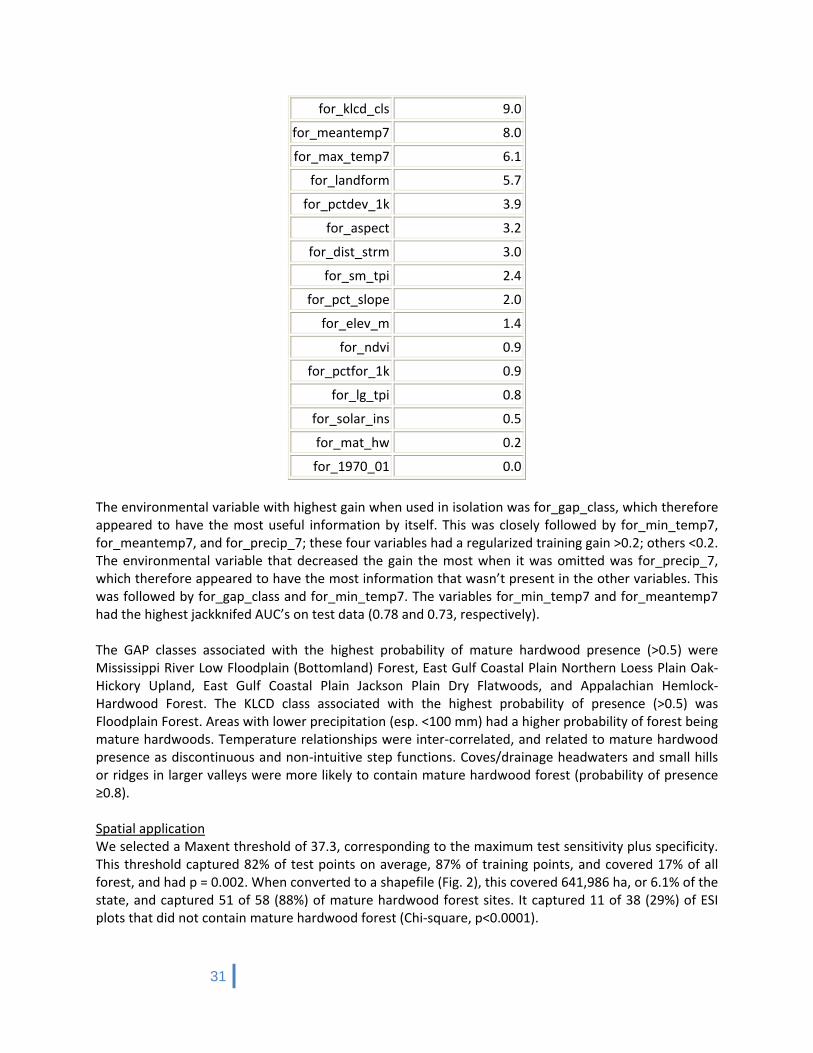
31
for_klcd_cls 9.0
for_meantemp7 8.0
for_max_temp7 6.1
for_landform 5.7
for_pctdev_1k 3.9
for_aspect 3.2
for_dist_strm 3.0
for_sm_tpi 2.4
for_pct_slope 2.0
for_elev_m 1.4
for_ndvi 0.9
for_pctfor_1k 0.9
for_lg_tpi 0.8
for_solar_ins 0.5
for_mat_hw 0.2
for_1970_01 0.0
The environmental variable with highest gain when used in isolation was for_gap_class, which therefore appeared to have the most useful information by itself. This was closely followed by for_min_temp7, for_meantemp7, and for_precip_7; these four variables had a regularized training gain >0.2; others <0.2. The environmental variable that decreased the gain the most when it was omitted was for_precip_7, which therefore appeared to have the most information that wasn’t present in the other variables. This was followed by for_gap_class and for_min_temp7. The variables for_min_temp7 and for_meantemp7 had the highest jackknifed AUC’s on test data (0.78 and 0.73, respectively). The GAP classes associated with the highest probability of mature hardwood presence (>0.5) were Mississippi River Low Floodplain (Bottomland) Forest, East Gulf Coastal Plain Northern Loess Plain Oak‐Hickory Upland, East Gulf Coastal Plain Jackson Plain Dry Flatwoods, and Appalachian Hemlock‐Hardwood Forest. The KLCD class associated with the highest probability of presence (>0.5) was Floodplain Forest. Areas with lower precipitation (esp. <100 mm) had a higher probability of forest being mature hardwoods. Temperature relationships were inter‐correlated, and related to mature hardwood presence as discontinuous and non‐intuitive step functions. Coves/drainage headwaters and small hills or ridges in larger valleys were more likely to contain mature hardwood forest (probability of presence ≥0.8). Spatial application We selected a Maxent threshold of 37.3, corresponding to the maximum test sensitivity plus specificity. This threshold captured 82% of test points on average, 87% of training points, and covered 17% of all forest, and had p = 0.002. When converted to a shapefile (Fig. 2), this covered 641,986 ha, or 6.1% of the state, and captured 51 of 58 (88%) of mature hardwood forest sites. It captured 11 of 38 (29%) of ESI plots that did not contain mature hardwood forest (Chi‐square, p<0.0001).
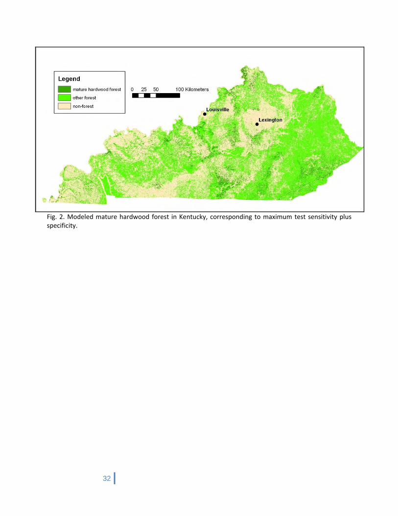
32
Fig. 2. Modeled mature hardwood forest in Kentucky, corresponding to maximum test sensitivity plus specificity.

33
Maxent Modeling of Mature Hardwood Forest
Ohio
December 3, 2010
Technical Contact: Ted Weber
The Conservation Fund 410 Severn Ave., Suite 204 Annapolis, Maryland 21403
410-990-0175 [email protected]
Methods Known locations of mature hardwood forest We selected mature forest from ESI forest surveys, based on mean canopy tree diameter (DBH), estimated stand age, species composition, successional stage, disturbance (e.g., logged areas were excluded unless minor impact), and overall score. Two points were missing coordinates and had to be omitted. We added other confirmed locations of mature or old‐growth hardwood forest collected by the Fund. From Wayne National Forest (WNF) stand data, we selected 36 mature hardwood forest stands according to stand descriptions and remarks. We only selected stands that clearly identified this in all fields, and did not select any stands that had been thinned or otherwise cut. We used aerial photos from ESRI (ESRI_Imagery_World_2D) to identify points in the center of these stands and surrounded by trees with large crown diameters. We omitted stands that had been logged or were small (e.g., road islands). We selected two points in some large stands, arriving at a total of 42 points. The above collections of forest data were restricted primarily to the southern half of the state, geographically biasing the model. We therefore added 11 points in northern Ohio in locations identified by Davis (2003) as old growth hardwood forest but had not been visited as part of this project, nor were in WNF. As with the WNF data, we used ESRI aerial photos to identify points in the center of these woods and surrounded by trees with large crown diameters. The subsequent distribution of 123 mature hardwood forest points and 30 non‐mature forest points more closely resembled a distribution of 153 randomly selected forest points (using Hawth’s Tools), than the distribution without them. We compared model results with and without the additional locations. Environmental variables We computed the variables in Table 1 within Ohio. We masked out non‐forest according to the 2001 National Land Cover Dataset (NLCD). We reprojected all layers to Albers equal area, with a grid cell size of 30 m. Table 1. Environmental variables computed in Ohio.

34
Variable Description
for_nlcd_cls Land cover classification from 2001 NLCD
for_gap_class Classified vegetation in 1999‐2002, from Ohio State Gap Analysis Project
for_1970_01 Forested in c.1970‐1985 (and still forested in 2001). Obtained from USGS; digitized from aerial photos and not entirely consistent with Landsat data.
for_pctfor_1k Percent forest within 1km
for_pctdev_1k Percent developed land within 1km
for_ndvi 250m MODIS Normalized Difference Vegetation Index, resampled to 30m, and scaled using the formula (NDVI * 200) + 50. Higher values indicate denser vegetation.
for_elev_m Elevation from USGS 30m DEMs in NHD+ dataset
for_pct_slope Percent slope calculated from DEM
for_aspect Aspect calculated from DEM
for_lg_tpi Topographic position index calculated in a 2010 m radius
for_sm_tpi Topographic position index calculated in a 510 m radius
for_landform Landform classification
for_max_temp7 Maximum July temperature from ClimateSource
for_min_temp7 Minimum July temperature from ClimateSource
for_meantemp7 Mean July temperature from ClimateSource
for_precip_7 Mean July rainfall from ClimateSource
for_insolat June insolation, calculated from 30m DEMs and latitude
for_dist_strm Distance to nearest stream (m)
Maxent model We used 10‐fold cross‐validation, which split the sample into ten different sets of 108‐109 training samples and 12‐13 test samples with the added northern points, and 99‐100 training samples and 11‐12 test samples without them. We set parameters as follows: • Output format = logistic • Use all possible variable relationships (linear, quadratic, product, threshold, and hinge) • Regularization multiplier = 1 • Maximum number of background points = 10,000 • Crossvalidate with 10 replicates • Add samples to background • Extrapolate • Do clamping • Maximum number of iterations = 500 • Convergence threshold = 0.00001 Spatial application We converted Maxent ASCII output to a floating point grid:
Arc: asciigrid mature_hardwood_forest_avg.asc flt_mat_hw float We multiplied this by 100 and took the integer value:

35
Grid: mature_hw_avg = int(flt_mat_hw * 100) We selected the Maxent threshold that captured the highest proportion of test points, while covering the least area of forest. Generally, this corresponds to the maximum test sensitivity plus specificity. We only considered thresholds with p<0.05. We reclassified the Maxent grid to a binary format (1 = above the threshold; 0 = below), and smoothed this by removing isolated areas <1 ac and filling holes <1 ac. We converted the resultant grid (OH_mature_hw) to a shapefile (OH_mature_hardwood_forest_from_Maxent.shp). Results Maxent model The Maxent model with the added northern points had a mean training AUC = 0.952, mean test AUC = 0.866 (std. dev. 0.029)). The Maxent model without the added northern points had a mean training AUC = 0.958, mean test AUC = 0.868 (std. dev. 0.049)). Figure 1 shows mean model output for all points. We preferred the model with all points even though the AUC was slightly (<1%) lower, because variance was much lower, and more northern mature forest locations corresponded to high Maxent predictions.
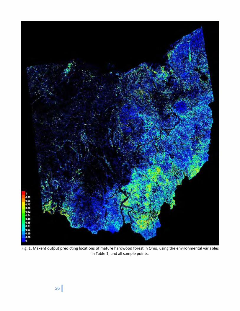
36
Fig. 1. Maxent output predicting locations of mature hardwood forest in Ohio, using the environmental variables
in Table 1, and all sample points.

37
Individual variable contributions Table 2 gives a heuristic estimate of relative contributions of the environmental variables to the Maxent model using all points. To determine the estimate, in each iteration of the training algorithm, the increase in regularized gain was added to the contribution of the corresponding variable, or subtracted from it if the change to the absolute value of lambda was negative. Variable contributions should be interpreted with caution. Values shown are averages over replicate runs.
Table 2. Individual variable contributions to the Maxent model.
Variable Percent contribution
for_1970_01 21.2
for_min_temp7 12.6
for_pctfor_1k 11.0
for_elev_m 10.0
for_ndvi 9.0
for_gap_class 5.8
for_max_temp7 5.3
for_precip_7 5.0
for_meantemp7 4.1
for_landform 3.0
for_sm_tpi 2.7
for_aspect 2.5
for_lg_tpi 1.8
for_pct_slope 1.8
for_pctdev_1k 1.4
for_dist_strm 1.4
for_insolat 1.2
for_nlcd_cls 0.2
The environmental variable with the highest training gain when used in isolation was for_1970_01, which therefore appeared to have the most useful information by itself. This was followed by for_min_temp7, for_pctfor_1k, for_ndvi, and for_gap_class (gain >0.2). The environmental variable that decreased the training gain the most when it was omitted was for_pctfor_1k, which therefore appeared to have the most information that wasn’t present in the other variables. This was followed by for_min_temp7. Only the variable for_min_temp7 had a jackknifed AUC >0.7 on test data. The variables for_ndvi, for_max_temp7, for_gap_class, for_elev_m, for_1970_01, and for_pctfor_1k had an AUC between 0.65 and 0.70. Table 3 lists the values associated with higher probabilities of mature hardwood forest presence, for variables that contributed >5% to the model. Variables were inter‐related, and combined in a variety of ways to create the model. Table 3. Values associated with higher probabilities of mature hardwood forest presence, for variables that contributed >5% to the model.
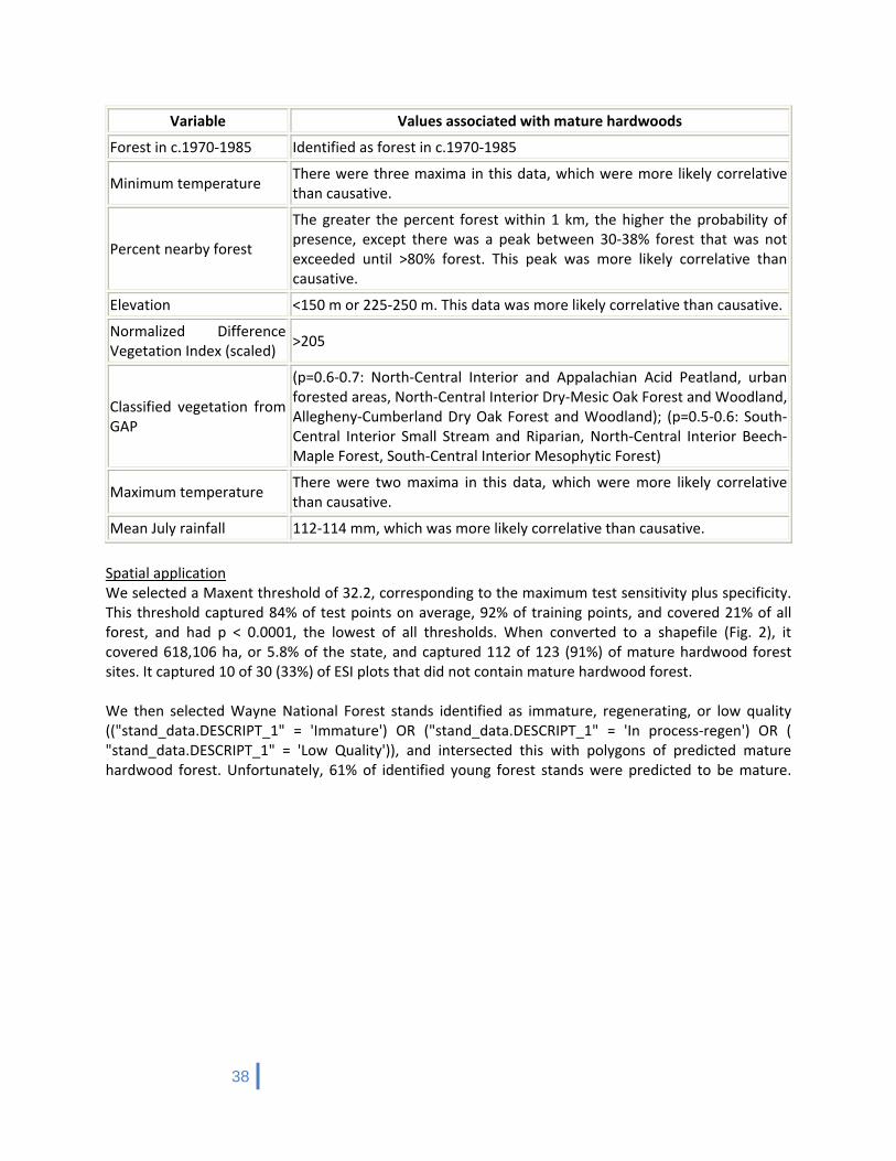
38
Variable Values associated with mature hardwoods
Forest in c.1970‐1985 Identified as forest in c.1970‐1985
Minimum temperature There were three maxima in this data, which were more likely correlative than causative.
Percent nearby forest
The greater the percent forest within 1 km, the higher the probability of presence, except there was a peak between 30‐38% forest that was not exceeded until >80% forest. This peak was more likely correlative than causative.
Elevation <150 m or 225‐250 m. This data was more likely correlative than causative.
Normalized Difference Vegetation Index (scaled)
>205
Classified vegetation from GAP
(p=0.6‐0.7: North‐Central Interior and Appalachian Acid Peatland, urban forested areas, North‐Central Interior Dry‐Mesic Oak Forest and Woodland, Allegheny‐Cumberland Dry Oak Forest and Woodland); (p=0.5‐0.6: South‐Central Interior Small Stream and Riparian, North‐Central Interior Beech‐Maple Forest, South‐Central Interior Mesophytic Forest)
Maximum temperature There were two maxima in this data, which were more likely correlative than causative.
Mean July rainfall 112‐114 mm, which was more likely correlative than causative.
Spatial application We selected a Maxent threshold of 32.2, corresponding to the maximum test sensitivity plus specificity. This threshold captured 84% of test points on average, 92% of training points, and covered 21% of all forest, and had p < 0.0001, the lowest of all thresholds. When converted to a shapefile (Fig. 2), it covered 618,106 ha, or 5.8% of the state, and captured 112 of 123 (91%) of mature hardwood forest sites. It captured 10 of 30 (33%) of ESI plots that did not contain mature hardwood forest. We then selected Wayne National Forest stands identified as immature, regenerating, or low quality (("stand_data.DESCRIPT_1" = 'Immature') OR ("stand_data.DESCRIPT_1" = 'In process‐regen') OR ( "stand_data.DESCRIPT_1" = 'Low Quality')), and intersected this with polygons of predicted mature hardwood forest. Unfortunately, 61% of identified young forest stands were predicted to be mature.
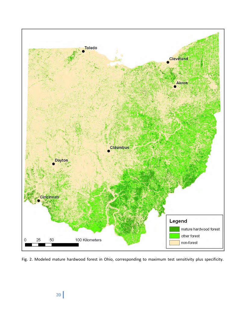
39
Fig. 2. Modeled mature hardwood forest in Ohio, corresponding to maximum test sensitivity plus specificity.

40
References Davis, M. B. 2003. Old growth in the East: a survey; revised edition. Appalachia‐Science in the Public Interest, Mount Vernon, KY. 273 pp.
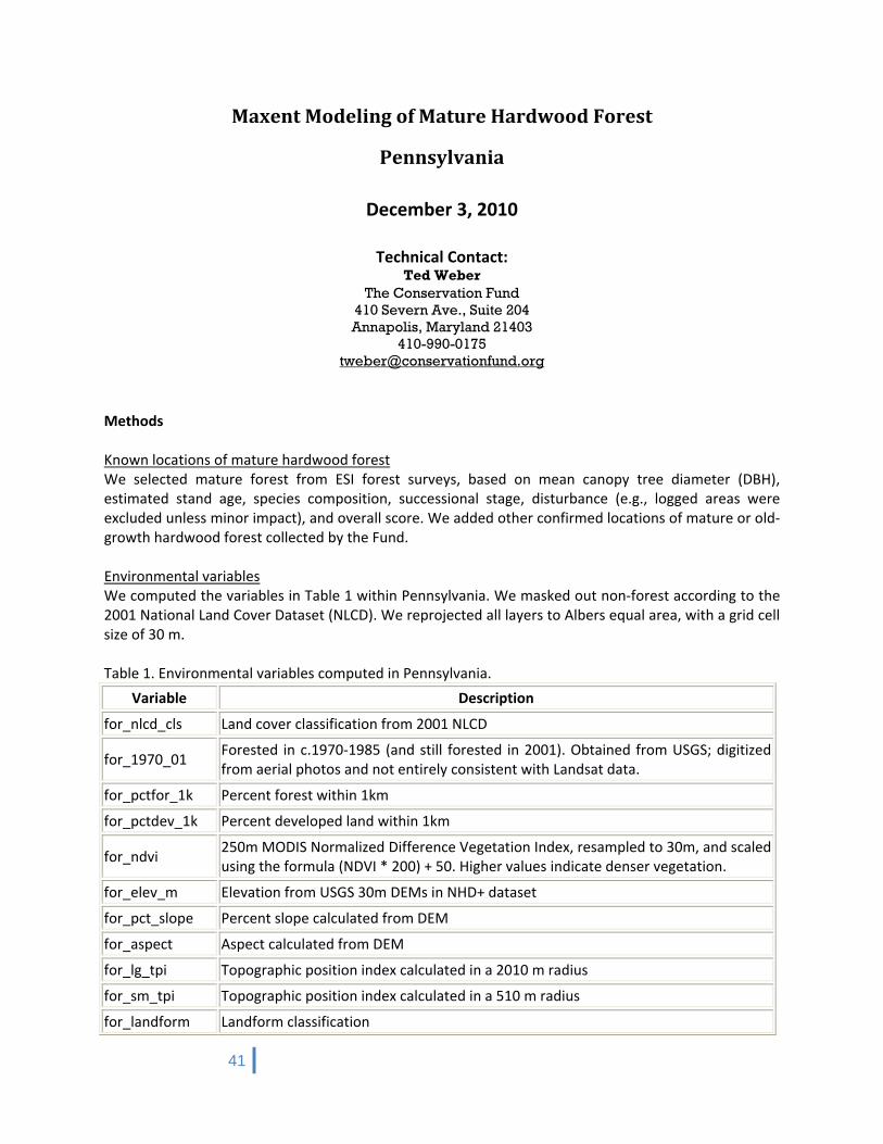
41
Maxent Modeling of Mature Hardwood Forest
Pennsylvania
December 3, 2010
Technical Contact: Ted Weber
The Conservation Fund 410 Severn Ave., Suite 204 Annapolis, Maryland 21403
410-990-0175 [email protected]
Methods Known locations of mature hardwood forest We selected mature forest from ESI forest surveys, based on mean canopy tree diameter (DBH), estimated stand age, species composition, successional stage, disturbance (e.g., logged areas were excluded unless minor impact), and overall score. We added other confirmed locations of mature or old‐growth hardwood forest collected by the Fund. Environmental variables We computed the variables in Table 1 within Pennsylvania. We masked out non‐forest according to the 2001 National Land Cover Dataset (NLCD). We reprojected all layers to Albers equal area, with a grid cell size of 30 m. Table 1. Environmental variables computed in Pennsylvania.
Variable Description
for_nlcd_cls Land cover classification from 2001 NLCD
for_1970_01 Forested in c.1970‐1985 (and still forested in 2001). Obtained from USGS; digitized from aerial photos and not entirely consistent with Landsat data.
for_pctfor_1k Percent forest within 1km
for_pctdev_1k Percent developed land within 1km
for_ndvi 250m MODIS Normalized Difference Vegetation Index, resampled to 30m, and scaled using the formula (NDVI * 200) + 50. Higher values indicate denser vegetation.
for_elev_m Elevation from USGS 30m DEMs in NHD+ dataset
for_pct_slope Percent slope calculated from DEM
for_aspect Aspect calculated from DEM
for_lg_tpi Topographic position index calculated in a 2010 m radius
for_sm_tpi Topographic position index calculated in a 510 m radius
for_landform Landform classification

42
for_max_temp7 Maximum July temperature from ClimateSource
for_min_temp7 Minimum July temperature from ClimateSource
for_meantemp7 Mean July temperature from ClimateSource
for_precip_7 Mean July rainfall from ClimateSource
for_insolat June insolation, calculated from 30m DEMs and latitude
for_dist_strm Distance to nearest stream (m)
Maxent model We used 10‐fold cross‐validation, which split the sample into ten different sets of 80‐81 training samples and 8‐9 test samples. We set parameters as follows: • Output format = logistic • Use all possible variable relationships (linear, quadratic, product, threshold, and hinge) • Regularization multiplier = 1 • Maximum number of background points = 10,000 • Crossvalidate with 10 replicates • Add samples to background • Extrapolate • Do clamping • Maximum number of iterations = 500 • Convergence threshold = 0.00001 Spatial application We converted Maxent ASCII output to a floating point grid:
Arc: asciigrid mature_hardwood_forest_avg.asc flt_mat_hw float We multiplied this by 100 and took the integer value:
Grid: mature_hw_avg = int(flt_mat_hw * 100) We selected the Maxent threshold that captured the highest proportion of test points, while covering the least area of forest. Generally, this corresponds to the maximum test sensitivity plus specificity. We only considered thresholds with p<0.05. We reclassified the Maxent grid to a binary format (1 = above the threshold; 0 = below), and smoothed this by removing isolated areas <1 ac and filling holes <1 ac. We converted the resultant grid (PA_mature_hw) to a shapefile (PA_mature_hardwood_forest_from_Maxent.shp). Results Maxent model The Maxent model had a mean training AUC = 0.908, mean test AUC = 0.802 (std. dev. 0.071)). Figure 1 shows mean model output.

43
Fig. 1. Maxent output predicting locations of mature hardwood forest in Pennsylvania, using the environmental variables in Table 1.

44
Individual variable contributions Table 2 gives a heuristic estimate of relative contributions of the environmental variables to the Maxent model. To determine the estimate, in each iteration of the training algorithm, the increase in regularized gain was added to the contribution of the corresponding variable, or subtracted from it if the change to the absolute value of lambda was negative. Variable contributions should be interpreted with caution. Values shown are averages over replicate runs.
Table 2. Individual variable contributions to the Maxent model.
Variable Percent contribution
for_pctfor_1k 27.1
for_1970_01 11.3
for_dist_strm 10.7
for_lg_tpi 9.1
for_min_temp7 6.1
for_max_temp7 5.6
for_insolat 4.9
for_sm_tpi 4.4
for_precip_7 4.4
for_ndvi 3.5
for_pctdev_1k 2.9
for_meantemp7 2.3
for_elev_m 2.3
for_landform 2.0
for_nlcd_cls 1.8
for_aspect 1.1
for_pct_slope 0.8
The environmental variable with the highest training gain when used in isolation was for_pctfor_1k, which therefore appeared to have the most useful information by itself. This was followed by for_lg_tpi, for_1970_01, and for_ndvi (gain >0.15). The environmental variable that decreased the training gain the most when it was omitted was for_pctfor_1k, which therefore appeared to have the most information that wasn't present in the other variables. Only the variable for_pctfor_1k had a jackknifed AUC >0.65 on test data. Table 3 lists the values associated with higher probabilities of mature hardwood forest presence, for variables that contributed >5% to the model. Variables were inter‐related, and combined in a variety of ways to create the model.
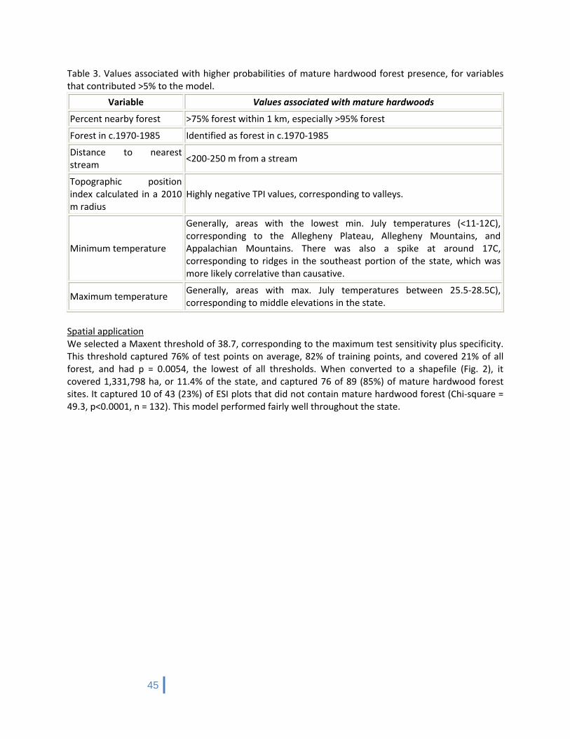
45
Table 3. Values associated with higher probabilities of mature hardwood forest presence, for variables that contributed >5% to the model.
Variable Values associated with mature hardwoods
Percent nearby forest >75% forest within 1 km, especially >95% forest
Forest in c.1970‐1985 Identified as forest in c.1970‐1985
Distance to nearest stream
<200‐250 m from a stream
Topographic position index calculated in a 2010 m radius
Highly negative TPI values, corresponding to valleys.
Minimum temperature
Generally, areas with the lowest min. July temperatures (<11‐12C), corresponding to the Allegheny Plateau, Allegheny Mountains, and Appalachian Mountains. There was also a spike at around 17C, corresponding to ridges in the southeast portion of the state, which was more likely correlative than causative.
Maximum temperature Generally, areas with max. July temperatures between 25.5‐28.5C), corresponding to middle elevations in the state.
Spatial application We selected a Maxent threshold of 38.7, corresponding to the maximum test sensitivity plus specificity. This threshold captured 76% of test points on average, 82% of training points, and covered 21% of all forest, and had p = 0.0054, the lowest of all thresholds. When converted to a shapefile (Fig. 2), it covered 1,331,798 ha, or 11.4% of the state, and captured 76 of 89 (85%) of mature hardwood forest sites. It captured 10 of 43 (23%) of ESI plots that did not contain mature hardwood forest (Chi‐square = 49.3, p<0.0001, n = 132). This model performed fairly well throughout the state.
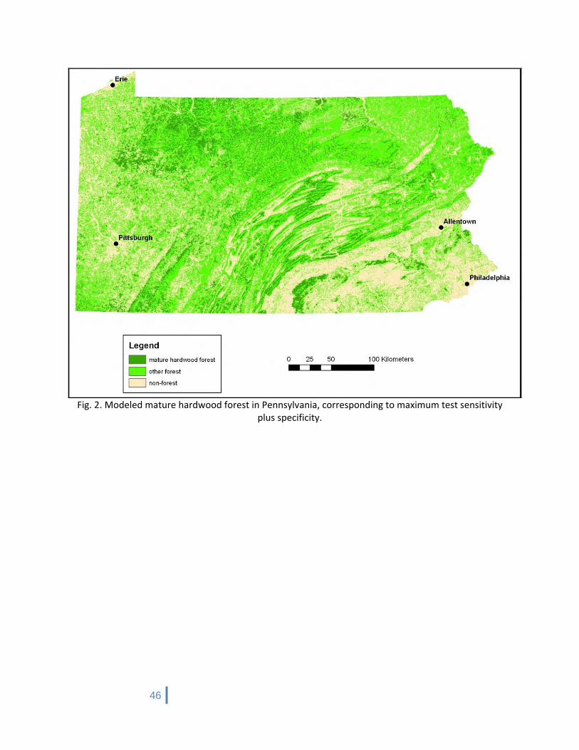
46
Fig. 2. Modeled mature hardwood forest in Pennsylvania, corresponding to maximum test sensitivity
plus specificity.
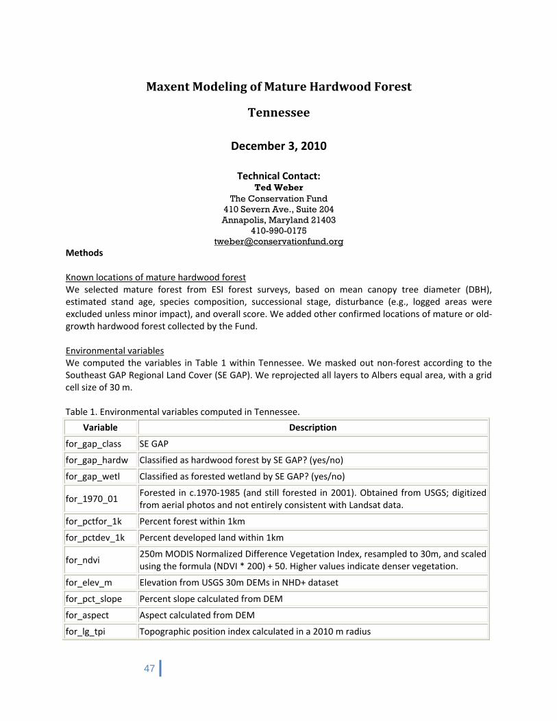
47
Maxent Modeling of Mature Hardwood Forest
Tennessee
December 3, 2010
Technical Contact: Ted Weber
The Conservation Fund 410 Severn Ave., Suite 204 Annapolis, Maryland 21403
410-990-0175 [email protected]
Methods Known locations of mature hardwood forest We selected mature forest from ESI forest surveys, based on mean canopy tree diameter (DBH), estimated stand age, species composition, successional stage, disturbance (e.g., logged areas were excluded unless minor impact), and overall score. We added other confirmed locations of mature or old‐growth hardwood forest collected by the Fund. Environmental variables We computed the variables in Table 1 within Tennessee. We masked out non‐forest according to the Southeast GAP Regional Land Cover (SE GAP). We reprojected all layers to Albers equal area, with a grid cell size of 30 m. Table 1. Environmental variables computed in Tennessee.
Variable Description
for_gap_class SE GAP
for_gap_hardw Classified as hardwood forest by SE GAP? (yes/no)
for_gap_wetl Classified as forested wetland by SE GAP? (yes/no)
for_1970_01 Forested in c.1970‐1985 (and still forested in 2001). Obtained from USGS; digitized from aerial photos and not entirely consistent with Landsat data.
for_pctfor_1k Percent forest within 1km
for_pctdev_1k Percent developed land within 1km
for_ndvi 250m MODIS Normalized Difference Vegetation Index, resampled to 30m, and scaled using the formula (NDVI * 200) + 50. Higher values indicate denser vegetation.
for_elev_m Elevation from USGS 30m DEMs in NHD+ dataset
for_pct_slope Percent slope calculated from DEM
for_aspect Aspect calculated from DEM
for_lg_tpi Topographic position index calculated in a 2010 m radius

48
for_sm_tpi Topographic position index calculated in a 510 m radius
for_landform Landform classification
for_max_temp7 Maximum July temperature from ClimateSource
for_min_temp7 Minimum July temperature from ClimateSource
for_meantemp7 Mean July temperature from ClimateSource
for_july_rain Mean July rainfall from ClimateSource
for_insolat June insolation, calculated from 30m DEMs and latitude
for_dist_strm Distance to nearest stream (m)
An earlier model included state geology data, but this was too coarse relative to the other data, so we omitted it. Earlier models also had incorrect coordinates for point #72, but this was corrected. Maxent model We used 10‐fold cross‐validation, which split the sample into ten different sets of 61‐62 training samples and 6‐7 test samples. We set parameters as follows: • Output format = logistic • Use all possible variable relationships (linear, quadratic, product, threshold, and hinge) • Regularization multiplier = 1 • Maximum number of background points = 10,000 • Crossvalidate with 10 replicates • Add samples to background • Extrapolate • Do clamping • Maximum number of iterations = 500 • Convergence threshold = 0.00001 We ran three alternative models. The first used the parameters listed above. The second used the same data and parameters, except with automatically selected variable relationships based on the number of sample points. The third used all possible variable relationships, but a regularization multiplier = 3. Spatial application We converted Maxent ASCII output to a floating point grid:
Arc: asciigrid mature_hardwood_forest_avg.asc flt_mat_hw float We multiplied this by 100 and took the integer value:
Grid: mature_hw_avg = int(flt_mat_hw * 100) We selected the Maxent threshold that captured the highest proportion of test points, while covering the least area of forest. Generally, this corresponds to the maximum test sensitivity plus specificity. We only considered thresholds with p<0.05. We reclassified the Maxent grid to a binary format (1 = above the threshold; 0 = below), and smoothed this by removing isolated areas <1 ac and filling holes <1 ac. We converted the resultant grid (TN_mature_hw) to a shapefile (TN_mature_hardwood_forest_from_Maxent.shp). Results

49
Maxent model The Maxent model using all possible variable relationships and a regularization multiplier = 1 had the best predictivity (mean training AUC = 0.955, mean test AUC = 0.799 (std. dev. 0.089)). Figure 1 shows mean model output. The second Maxent model, with automatically selected variable relationships based on the number of sample points, was less satisfactory. Maxent tested linear, quadratic, and hinge relationships (i.e., did not consider product or threshold); the resultant model had an average training AUC of 0.892 and test AUC of 0.786 (std. dev. 0.081). The third model, using all possible variable relationships, but a regularization multiplier = 3, was the least satisfactory, with a training AUC of 0.844 and average test AUC of 0.774 (std. dev. 0.072).
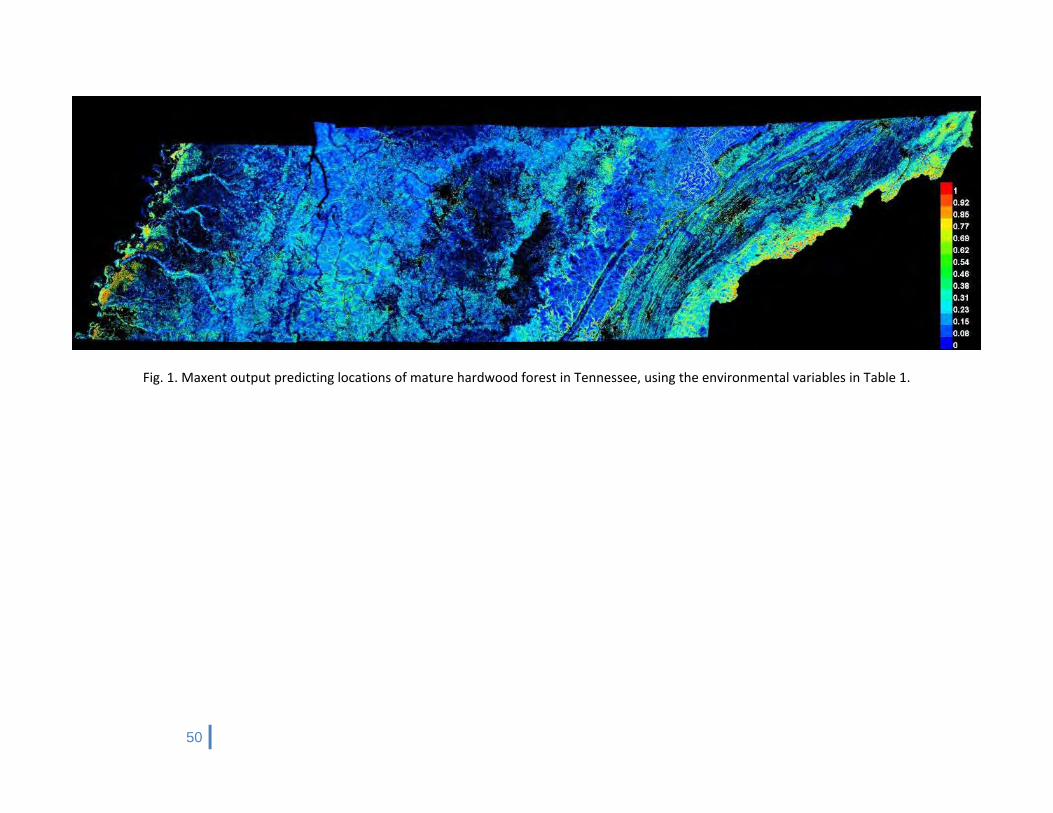
50
Fig. 1. Maxent output predicting locations of mature hardwood forest in Tennessee, using the environmental variables in Table 1.
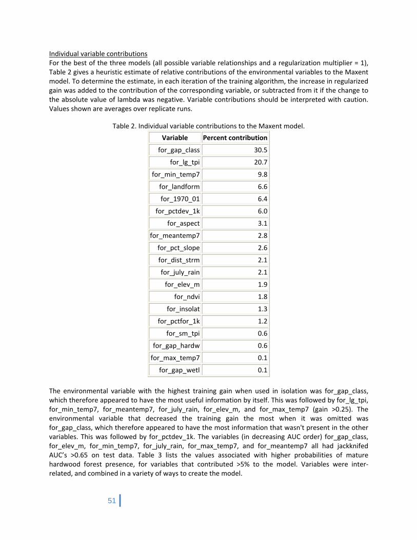
51
Individual variable contributions For the best of the three models (all possible variable relationships and a regularization multiplier = 1), Table 2 gives a heuristic estimate of relative contributions of the environmental variables to the Maxent model. To determine the estimate, in each iteration of the training algorithm, the increase in regularized gain was added to the contribution of the corresponding variable, or subtracted from it if the change to the absolute value of lambda was negative. Variable contributions should be interpreted with caution. Values shown are averages over replicate runs.
Table 2. Individual variable contributions to the Maxent model.
Variable Percent contribution
for_gap_class 30.5
for_lg_tpi 20.7
for_min_temp7 9.8
for_landform 6.6
for_1970_01 6.4
for_pctdev_1k 6.0
for_aspect 3.1
for_meantemp7 2.8
for_pct_slope 2.6
for_dist_strm 2.1
for_july_rain 2.1
for_elev_m 1.9
for_ndvi 1.8
for_insolat 1.3
for_pctfor_1k 1.2
for_sm_tpi 0.6
for_gap_hardw 0.6
for_max_temp7 0.1
for_gap_wetl 0.1
The environmental variable with the highest training gain when used in isolation was for_gap_class, which therefore appeared to have the most useful information by itself. This was followed by for_lg_tpi, for_min_temp7, for_meantemp7, for_july_rain, for_elev_m, and for_max_temp7 (gain >0.25). The environmental variable that decreased the training gain the most when it was omitted was for_gap_class, which therefore appeared to have the most information that wasn't present in the other variables. This was followed by for_pctdev_1k. The variables (in decreasing AUC order) for_gap_class, for_elev_m, for_min_temp7, for_july_rain, for_max_temp7, and for_meantemp7 all had jackknifed AUC’s >0.65 on test data. Table 3 lists the values associated with higher probabilities of mature hardwood forest presence, for variables that contributed >5% to the model. Variables were inter‐related, and combined in a variety of ways to create the model.
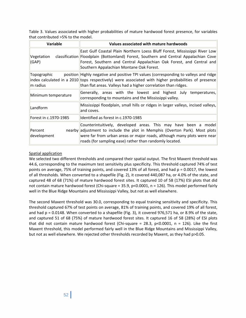
52
Table 3. Values associated with higher probabilities of mature hardwood forest presence, for variables that contributed >5% to the model.
Variable Values associated with mature hardwoods
Vegetation classification (GAP)
East Gulf Coastal Plain Northern Loess Bluff Forest, Mississippi River Low Floodplain (Bottomland) Forest, Southern and Central Appalachian Cove Forest, Southern and Central Appalachian Oak Forest, and Central and Southern Appalachian Montane Oak Forest.
Topographic position index calculated in a 2010 m radius
Highly negative and positive TPI values (corresponding to valleys and ridge tops respectively) were associated with higher probabilities of presence than flat areas. Valleys had a higher correlation than ridges.
Minimum temperature Generally, areas with the lowest and highest July temperatures, corresponding to mountains and the Mississippi valley.
Landform Mississippi floodplain, small hills or ridges in larger valleys, incised valleys, and coves.
Forest in c.1970‐1985 Identified as forest in c.1970‐1985
Percent nearby development
Counterintuitively, developed areas. This may have been a model adjustment to include the plot in Memphis (Overton Park). Most plots were far from urban areas or major roads, although many plots were near roads (for sampling ease) rather than randomly located.
Spatial application We selected two different thresholds and compared their spatial output. The first Maxent threshold was 44.6, corresponding to the maximum test sensitivity plus specificity. This threshold captured 74% of test points on average, 75% of training points, and covered 13% of all forest, and had p = 0.0017, the lowest of all thresholds. When converted to a shapefile (Fig. 2), it covered 440,087 ha, or 4.0% of the state, and captured 48 of 68 (71%) of mature hardwood forest sites. It captured 10 of 58 (17%) ESI plots that did not contain mature hardwood forest (Chi‐square = 35.9, p<0.0001, n = 126). This model performed fairly well in the Blue Ridge Mountains and Mississippi Valley, but not as well elsewhere. The second Maxent threshold was 30.0, corresponding to equal training sensitivity and specificity. This threshold captured 67% of test points on average, 81% of training points, and covered 19% of all forest, and had p = 0.0148. When converted to a shapefile (Fig. 3), it covered 976,571 ha, or 8.9% of the state, and captured 51 of 68 (75%) of mature hardwood forest sites. It captured 16 of 58 (28%) of ESI plots that did not contain mature hardwood forest (Chi‐square = 28.3, p<0.0001, n = 126). Like the first Maxent threshold, this model performed fairly well in the Blue Ridge Mountains and Mississippi Valley, but not as well elsewhere. We rejected other thresholds recorded by Maxent, as they had p>0.05.
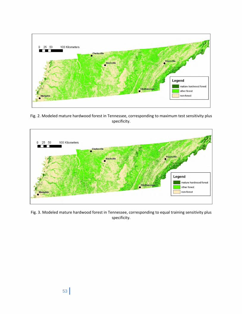
53
Fig. 2. Modeled mature hardwood forest in Tennessee, corresponding to maximum test sensitivity plus specificity.
Fig. 3. Modeled mature hardwood forest in Tennessee, corresponding to equal training sensitivity plus specificity.