
Field Methods Manual: US Fish and Wildlife Service (Region
67
Field Methods Manual: US Fish and Wildlife Service (Region 5) salt marsh study Mary-Jane James-Pirri Graduate School of Oceanography University of Rhode Island Narragansett, RI 02882 [email protected] Charles T. Roman 1 USGS Patuxent Wildlife Research Center Graduate School of Oceanography University of Rhode Island Narragansett, RI 02882 [email protected] R. Michael Erwin USGS Patuxent Wildlife Research Center Department of Environmental Sciences University of Virginia Charlottesville, VA 22903 [email protected] 1 Present address: National Park Service Graduate School of Oceanography University of Rhode Island Narragansett, RI 02882 April 2002 (version 2) USGS Patuxent Wildlife Research Center Coastal Research Field Station
Transcript of Field Methods Manual: US Fish and Wildlife Service (Region

Field Methods Manual: US Fish and Wildlife Service (Region 5) salt marsh
study
Mary-Jane James-Pirri Graduate School of Oceanography
University of Rhode Island Narragansett, RI 02882
Charles T. Roman 1USGS Patuxent Wildlife Research Center
Graduate School of Oceanography University of Rhode Island
Narragansett, RI 02882 [email protected]
R. Michael Erwin USGS Patuxent Wildlife Research Center Department of Environmental Sciences
University of Virginia Charlottesville, VA 22903
1 Present address: National Park Service Graduate School of Oceanography
University of Rhode Island Narragansett, RI 02882
April 2002 (version 2)
USGS Patuxent Wildlife Research Center
Coastal Research Field Station

Monitoring Protocols
ii

Monitoring Protocols
iii
TABLE OF CONTENTS Table of Contents ............................................................................................................. iii List of Figures ................................................................................................................... v List of Tables .................................................................................................................... v Introduction ...................................................................................................................... 1 General study design ........................................................................................................ 2 Vegetation ......................................................................................................................... 4 Materials for site selection and location of vegetation plots ................................... 4
Site selection and sample location .......................................................................... 4 Materials for sampling permanent vegetation plots ................................................ 7 Sampling procedure ................................................................................................ 7
Water table level .............................................................................................................. 12 Materials for ground water wells ........................................................................... 12 Groundwater well fabrication ................................................................................ 12 Well installation ..................................................................................................... 13 Materials for sampling ground water wells ............................................................ 13 Sampling procedure ............................................................................................... 14
Soil salinity ...................................................................................................................... 15 Materials for soil salinity ........................................................................................ 15 Soil probe fabrication ............................................................................................. 15 Sample procedure ................................................................................................... 16 Soil sulfides ...................................................................................................................... 19
Materials for soil sulfides........................................................................................ 19 Sampling procedure ................................................................................................ 19
Mosquito larvae ............................................................................................................... 20 Materials for mosquito sampling ............................................................................ 20 Sampling procedure ................................................................................................ 20 Methods to preserve mosquito larvae ..................................................................... 22
Nekton in ponds ............................................................................................................... 24 Materials for location of pond stations ................................................................... 24 Nekton pond station location procedure ................................................................. 24 Materials for construction of throw trap ................................................................. 25 Materials for construction of dip net ....................................................................... 25 Throw trap and dip net fabrication .......................................................................... 26 Materials for sampling nekton in ponds.................................................................. 28 Sampling procedure ................................................................................................ 28
Nekton in ditches ............................................................................................................. 32 Materials for location of ditch stations ................................................................... 32 Nekton ditch station location procedure ................................................................. 32 Materials for construction of ditch net .................................................................... 33 Ditch net fabrication ............................................................................................... 33 Materials for sampling nekton in ditches ................................................................ 36 Sampling procedure ................................................................................................ 36

Monitoring Protocols
iv
Calculating the area of the ditch net ....................................................................... 38 Bird Surveys..................................................................................................................... 41
Methods: Group 1 Species ...................................................................................... 41 Methods: Group 2 and 3 Species ............................................................................ 42 Training ................................................................................................................... 43 Instructions for filling out bird survey data form .................................................... 44
Other environmental variables ......................................................................................... 49 Data management............................................................................................................. 50 Data Headers for spreadsheets ......................................................................................... 51 Vegetation ............................................................................................................... 52 Water table level and soil salinity ........................................................................... 53 Mosquito data headers ............................................................................................ 53 Nekton data headers ................................................................................................ 54 Bird Survey data headers ........................................................................................ 54 Literature Cited ................................................................................................................ 56 Field Identification Resources ......................................................................................... 58 Contact Information ......................................................................................................... 60

Monitoring Protocols
v
LIST OF FIGURES
1. Photo of transect and plot layout from Prime Hook NWR ........................................... 6 2. Diagram of quadrat orientation relative to plot stake ................................................... 7 3. Diagram of the sample quadrat and arrangement of dowels......................................... 9 4. Diagram of location of groundwater wells ................................................................. 13 5. Diagram of water table well ........................................................................................ 14 6. Photo of soil probe ....................................................................................................... 16 7. Photo of throw trap and dip net.................................................................................... 27 8. Photo showing method to toss throw trap .................................................................... 30 9a &b. Schematic of ditch net .......................................................................................... 35 10a-c. Photo of ditch net deployed in field ...................................................................... 39
LIST OF TABLES
1. Example data sheet for the point intercept method ...................................................... 10 2. Cover type categories for point-intercept method ....................................................... 11 3. Example data sheet for water table level and soil salinity method ............................. 18 4. Example data sheet for mosquito larvae method ......................................................... 23 5. Example data sheet for throw trap method .................................................................. 31 6. Example data sheet for ditch net method ..................................................................... 40 7. Example of bird survey data sheet ............................................................................... 47 8. Site codes for refuges and study areas ......................................................................... 51 9. Example of vegetation data entry format ..................................................................... 52 10. Example of water table level and soil salinity data entry format ............................... 53 11. Example of mosquito data entry format..................................................................... 55 12. Example of nekton station data entry format ............................................................. 55 13. Example of individual nekton data entry format ....................................................... 55

Monitoring Protocols
1
INTRODUCTION
Salt marshes are a common ecosystem type within coastal Refuges of the US Fish and Wildlife Service from Maine to Virginia (Region 5). Most of these marshes have been parallel ditched for mosquito control purposes, and to a lesser extent, to facilitate salt hay farming. Although ditching of salt marshes has occurred since Colonial times, most extensive ditching was in the 1930s, with programs to maintain ditches continuing for three decades or more. Documented impacts of parallel ditching on salt marshes include lowered water table levels, drainage of marsh pools and panes, vegetation changes, and associated impacts on habitat support functions for fish, birds, and other trophic components. Recognizing the detrimental impacts associated with ditching, the practice of Open Marsh Water Management (OMWM), considered a more ecologically appropriate mosquito control method, was introduced in the late 1960s. OMWM is a common practice on coastal Refuges, especially in New Jersey (Forsythe NWR) and Delaware (Prime Hook NWR). In brief, OMWM involves physical alteration of the parallel ditched marsh, through creation of pools and other hydrologic alterations, to establish a marsh that is unsuitable for mosquito egg deposition and larval development, and that promotes establishment of habitats for larvivorous fishes. Traditional OMWM includes plugging of ditches, creation/excavation of ponds within intense breeding areas, construction of radial ditches to facilitate fish access to breeding areas, and other manipulations. As noted, traditional OMWM practices are common at Forsythe and Prime Hook NWR. At more northern Refuges (Long Island Complex, S.B. McKinney, Parker River, and Rachel Carson) a modification of OMWM is being implemented, which is generally limited to ditch plugging, with limited or no pond excavation and radial ditches. The objective of ditch plugging is to re-establish a hydrologic regime on the ditched marsh that is characterized by permanent water on the marsh surface, thereby restoring fish and wildlife habitat functions while controlling mosquito production. A cooperative research project of the USGS-Patuxent Wildlife Research Center and US FWS-Region 5 was initiated in 2001 to quantitatively evaluate the response of salt marshes to OMWM and associated practices. The objectives of the three year study are to compare parallel ditched salt marshes with OMWM marshes. Specifically, this study is designed to evaluate the effects of OMWM and/or ditch plugging on marsh hydrology (marsh water table levels, soil salinity, and extent of surface water flooding), sedimentation and marsh development processes, vegetation patterns, utilization by nekton (fish and decapod crustaceans) and birds, and mosquito control. Research study sites were established at Rachel Carson NWR (ME) in 1999. Parker River NWR (MA), Long Island Complex (Wertheim NWR, NY), and Prime Hook NWR (DE) were established in 2001. Research will begin at Forsythe NWR (NJ) in 2002 and at Stewart B. McKinney (CT) in 2002/03. The purpose of this document is to serve as a Field Methods Manual for the study. Details are provided on how to collect and record the data on appropriate field data sheets. Guidelines on data management, at least with respect to entering data into spreadsheets, are also provided. This manual does not address data analysis techniques. This document is

Monitoring Protocols
2
presented as Version 1 of the Fields Methods Manual. Subsequent versions will include marsh sedimentation methods as well as minor modifications as needed.
GENERAL STUDY DESIGN
This study employs a BACI study design (before, after, control, impact). At each study Refuge we have (or will) selected pairs of sites that include a ditched marsh and a control marsh. The ditched marsh and control marsh are sampled for one year prior to any OMWM activities (Before). Then in year two, OMWM is performed on the ditched marsh and sampling proceeds (After). In the BACI design, the practice of OMWM is the “impact.” With this kind of study design it is possible to evaluate, with a degree of statistical certainty, the initial response of the marsh to OMWM. Continued monitoring in successive years will track the long-term response of the marsh to OMWM. It is important to monitor the control marsh simultaneously with sampling the ditched/OMWM marsh. If after OMWM a particular parameter such as water table level changed, and water level did not change in the control marsh, then it could be suggested with some degree of certainty that the change in water table was due to the OMWM and not some other factors. Inclusion of a control marsh serves to document any changes that are occurring in response to regional or local factors that are independent of OMWM manipulations. To date, the following study sites have been established. Experimental refers to the OMWM or ditch-plugged marsh. Control and Experimental study areas vary in area, ranging from 0.6ha to 12.2ha. Rachel Carson NWR
• Granite Point Rd. Marsh (control and experimental) • Moody Marsh (control and experimental) • Marshall Point Rd. Marsh (control and experimental)
Parker River NWR
• Control • Experimental B1 • Experimental B2 • Experimental A
Long Island Complex
• Wertheim East experimental and Smith County Park control • Flanders (control and experimental)
Forsythe NWR
• Oyster Creek, Atlantic County (control and experimental) • AT&T, Ocean County (control and experimental)

Monitoring Protocols
3
Prime Hook NWR • Petersfield Ditch (control and experimental) • Slaughter Beach (control and experimental)

Monitoring Protocols
4
VEGETATION
SUMMARY The salt marsh vegetation monitoring protocol recommends sampling vegetation community composition and abundance with permanent plots using the point intercept method. At least 20 vegetation plots are required per study area to detect differences in community composition and abundance. Permanent quadrats should be arranged in transects and spaced a minimum of 10-20m apart to maintain independence. Transects should be randomly located within each study area with the first permanent plot randomly located and subsequent plots systematically placed along each transect. Vegetation is sampled once during a season, usually at the end of the growing season (late summer or early fall) when plants are easily identifiable. At least 2 people are required to sample vegetation, one to place the bayonet and the other to record data. It is estimated that 2 people, who are familiar with salt marsh plant identifications, can sample approximately 10-20 plots per day. This does not include time spent re-locating plots that have lost their stakes. Details of the salt marsh vegetation monitoring protocol, including justification of the suggested field method and sample size, are found in Roman et al. (2001). Materials for Site Selection and Location of Vegetation Plots
• Oak stakes to mark vegetation plots • Mallet to pound stakes into ground • Black permanent markers to mark transect and plot number on stakes • Compass • Meter tape (preferably 100m long) • Random number table • Aerial photos of study sites • Draft map of study site showing boundaries of study areas and approximate location of
transects Site Selection and Sample Location
• Define boundaries of the control and experimental areas. • Systematically divide each study area into segments to adequately sample the marsh.
Segmentation is done to insure dispersion of the vegetation plots throughout the study area. Usually, a study area is segmented into 3 or 4 similarly sized areas.
• Randomly locate transects that traverse the main gradient (e.g., elevation) from creek bank to upland edge of the marsh. The starting point for each transect is randomly located along the creek bank. The random location of the starting point for each transect is selected by measuring the total distance of the creek bank (within each segment) and then randomly selecting points along the bank where each transect will start. These measurements are best done from aerial photography.

Monitoring Protocols
5
• There is no definitive number of transects that should be established per marsh segment, however each transect should be at least 10m apart, to maintain independence of the replicate plots. Transects be dispersed throughout the study areas to ensure that the vegetation plots are representative of the entire study area.
• All transects within a marsh segment should be parallel to each other (i.e., should run along the same compass heading) for ease in re-locating plots.
• Locate vegetation plots along each transect. Regardless of the size of the area a minimum of 20 plots are required for each study area.
• The first plot of each transect is randomly located within the low marsh zone. Measure the width of the low marsh and then place the plot at the distance selected by the random number (0 being on the edge of the bank). For example, if the low marsh zone is 5m wide, a random number between 0-5 would be selected. If there is no discernable low marsh zone, or if the vegetation zone at the creek bank is very broad, (i.e., more than 10m), then the first plot should be located by a random number between 0 and 10.
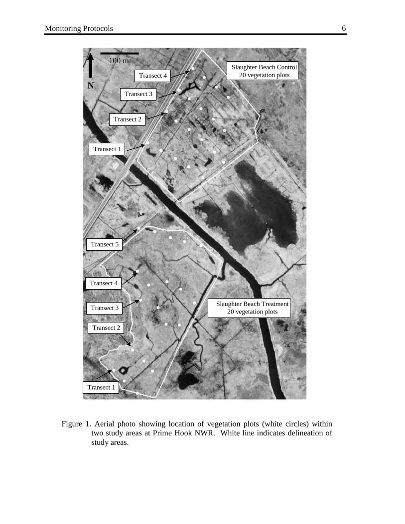
• After the first plot is located, all subsequent plots are then systematically placed, at least 10m apart, along the length of the transect. The spacing of plots along each transect will be variable depending on the area of the marsh. For example, if the marsh is 8-9 hectares in area, then 4 transects, with 40m spacing between plots along each transect would be appropriate. For smaller marshes, 20m spacing between plots may be necessary. However, all plots should be at least 10m apart to maintain independence of the replicate plots. (refer to Fig 1.).
• Each plot should be marked with stakes labeled clearly with transect and plot number. Construction of permanent stakes is at the discretion of the investigator. Our experience suggests that 4 ft oak stakes (1 ft into the marsh sediment, 3 ft above marsh; about 12 inch square) are adequate. Naming convention for vegetation plots is the transect number followed by the distance along the transect where the plot is located. For example, 1-00 would be the first plot on transect 1 (00 meters along the transect), 1-20 would be a plot on transect 1 located 20m from the start of the transect.
• Plot location and distance between plots should be carefully noted on a map so that plots can be re-located in future surveys in the event that the stake is missing. The coordinates (latitude and longitude, UTM coordinates, etc.) of all plots should be recorded, preferably with a GPS unit that has sub-meter accuracy.
Monitoring Protocols
6
Figure 1. Aerial photo showing location of vegetation plots (white circles) within two study areas at Prime Hook NWR. White line indicates delineation of study areas.
Transect 1
Transect 2
Transect 3
Transect 4 Slaughter Beach Control
20 vegetation plots
Slaughter Beach Treatment 20 vegetation plots
Transect 1
Transect 2
Transect 3
Transect 4
Transect 5
100 m
N

Monitoring Protocols
7
Materials for Sampling Permanent Vegetation Plots
• 1 m2 quadrat. The quadrat can be made from four 1m lengths of thin diameter (3-5mm) doweling. Dowels should be marked with 10 evenly spaced (11.1 cm apart) increments
• Bayonet or thin rod for point intercept method (less than 3mm diameter). • Meter stick • Map of vegetation plots • Plant identification book • Plastic bags for voucher specimens • Data sheet and pencils (Table 1)
Sampling Procedure
• Locate permanent stake marking the vegetation plot. • In order to sample vegetation that has not been trampled during the establishment of
transects, the quadrat is offset 1m from the stake. • Facing the direction of the transect (from the first plot towards the remaining plots of
the transect) set the quadrat 1m to the right of the stake and orient the plot towards the direction of the transect. Be sure to maintain the same offset for all plots and record a detailed description of the offset (Fig. 2). Note: if existing plots are oriented differently that is acceptable. Continue with the existing layout, but be certain to carefully document the orientation with a schematic such as that shown in Fig. 2.
Plot
Creek
Stake
Transect Line
1 m
Upland
Figure 2. A schematic of the orientation of the sampling quadrat relative to plot stake.

Monitoring Protocols
8
• A meter stick is placed on the marsh surface and then at 0, 25, 50, 75, and 100cm intervals along the meter stick, dowels (<3mm in diameter) are placed perpendicular to the meter stick. Each dowel is 1m in length and has a total of 10 marks, each spaced 11.1cm apart (Fig. 3). Thus, the 1m2 quadrat is divided into a grid of 50 evenly spaced points. In dense vegetation it may be necessary to weave the dowels through the vegetation.
• List all species that are present within the sample quadrat on the data sheet for that plot (a sample data sheet is presented in Table 1).
• Hold a thin rod (<3mm in diameter) vertical to the first sampling point and lower the rod through the vegetation canopy to the sample point on the ground.
• All species that touch the rod are recorded as a “hit” on the data sheet for that point. Categories other than plant species, such as “water”, “bare ground”, “wrack or litter,” and others are also recorded if they are “hit” by the rod. Table 2 provides definitions of cover type categories that should be included.
• More than one cover type category can touch the rod at each point, and thus multiple hits for each sample point should be recorded if appropriate. However, it is not necessary to count the number of hits for each individual species. For example, if S. alterniflora touches the rod in 3 places, it is recorded as one hit of S. alterniflora for that point. At least one cover type should be recorded for each point (i.e. if there is no vegetation, “bare ground” or “water” may be the appropriate cover type).
• After the first point is completed, the process is repeated for all remaining points on the sampling quadrat until all 50 points have been sampled.
• Tally the total number of hits per species for each plot on the data sheet (Table 1). This can be done after returning to the laboratory.
• All marsh study areas should be sampled within the same time frame (within 1-2 weeks of each other) and occur when the marsh surface is not flooded so that tidal waters do not conceal vegetation.
• This method can also be successfully used in marshes with taller vegetation canopies, like Phragmites and Typha marshes, or marshes dominated by shrubs (e.g., Iva). The observer needs to be careful to use a long rod and to look up to determine if higher vegetation touches the rod.

Monitoring Protocols
9
Figure 3. Schematic and photo of the sample quadrat and arrangement of dowels used in the point intercept method.
Meter stick Dowels with graduated marks
First sample point at 0,0
Direction of transect
Dowels with graduated markings
Direction of Transect
Plot stake First sample point at 0cm in direction of transect and 0cm into plot.
0 cm
25 cm
75 cm
50 cm
100 cm

Monitoring Protocols
10
Table 1. Example of a field data sheet for the point intercept method.
Marsh __________________ Field Crew ___________________ Date _______________________
Transect & Plot number __________________ GPS Coordinates N:___________________ E:___________________
Record species, first row is for points 1-25, second row is for points 26-50.
Point
SPECIES Total Tally
1
26
2 3 4 5
30
6 7 8 9 10
35
11 12 13 14 15
40
16 17 18 19 20
45
21 22 23 24 25
50
1.
Species # 1 -- pts. 26-50 XXXX
2
Species # 2 -- pts. 26-50 XXXX
3
Species # 3 -- pts. 26-50 XXXX
4
Species # 4 -- pts. 26-50 XXXX
5
Species # 5 -- pts. 26-50 XXXX
6
Species # 6 -- pts. 26-50 XXXX
7
Species # 7 -- pts. 26-50 XXXX
8.
Species # 8 -- pts. 26-50 XXXX
9.
Species # 9 -- pts. 26-50 XXXX
Monitoring Protocols
11
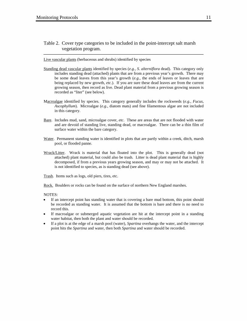
Table 2. Cover type categories to be included in the point-intercept salt marsh vegetation program.
Live vascular plants (herbaceous and shrubs) identified by species Standing dead vascular plants identified by species (e.g., S. alterniflora dead). This category only
includes standing dead (attached) plants that are from a previous year’s growth. There may be some dead leaves from this year’s growth (e.g., the ends of leaves or leaves that are being replaced by new growth, etc.). If you are sure these dead leaves are from the current growing season, then record as live. Dead plant material from a previous growing season is recorded as “liter” (see below).
Macroalgae identified by species. This category generally includes the rockweeds (e.g., Fucus,
Ascophyllum). Microalgae (e.g., diatom mats) and fine filamentous algae are not included in this category.
Bare. Includes mud, sand, microalgae cover, etc. These are areas that are not flooded with water
and are devoid of standing live, standing dead, or macroalgae. There can be a thin film of surface water within the bare category.
Water. Permanent standing water is identified in plots that are partly within a creek, ditch, marsh
pool, or flooded panne. Wrack/Litter. Wrack is material that has floated into the plot. This is generally dead (not
attached) plant material, but could also be trash. Litter is dead plant material that is highly decomposed, if from a previous years growing season, and may or may not be attached. It is not identified to species, as is standing dead (see above).
Trash. Items such as logs, old piers, tires, etc. Rock. Boulders or rocks can be found on the surface of northern New England marshes. NOTES: • If an intercept point has standing water that is covering a bare mud bottom, this point should
be recorded as standing water. It is assumed that the bottom is bare and there is no need to record this.
• If macroalgae or submerged aquatic vegetation are hit at the intercept point in a standing water habitat, then both the plant and water should be recorded.
• If a plot is at the edge of a marsh pool (water), Spartina overhangs the water, and the intercept point hits the Spartina and water, then both Spartina and water should be recorded.

Monitoring Protocols
12
WATER TABLE LEVEL
SUMMARY Water table level provides information on the amount of waterlogging or drainage that is occurring in a marsh. Water table level is an important parameter to use when attempting to understand why vegetation is changing. Water table level is measured using ground water wells. It is recommended that a water table level well be placed in association with each vegetation sampling plot. For water table level and soil salinity, approximately 20-30 sample stations could be visited within a low tide period. Sampling can be accomplished by one person, but teams of people are always recommended when conducting field work. More details on water table monitoring are found in Roman et al. (2001) Construction and installation of the wells is outlined below. Wells can also be purchased, pre-made, from hydrological supply companies. Materials for Groundwater Wells
• 1.5 inch (4 cm) interior diameter, schedule 40, PVC Tubes (comes in 10ft
lengths and can be purchased at home goods stores) • PVC caps to fit the tubes. Two caps (rounded preferably) are required for each
well • ¼ inch drill bit • Meter sticks • Black permanent markers to mark well number on caps • Mallets to pound wells into ground and blocks of wood to place on well top when
wells are pounded • All weather copier paper for field data sheets
Groundwater Well Fabrication • Cut PVC into 70 cm lengths (4 wells per 10 ft of tube), 10 cm will be
aboveground, 60cm will be belowground. • Drill ¼ inch holes in the belowground section of the well (along the 10–60cm
length of the well). Drill enough holes to allow water to percolate into the well. The top of the well is the 0-10cm section that has no drill holes; the bottom of the well is the section with the drill holes. To prevent surface water from entering the well the top 0-10cm section of the well is left intact.
• Place a cap on the bottom of each well. Well bottoms should fit snugly, but do not need to be glued.
• Draw a line 10cm down from the top of the well. In the field, this line will serve as a guide for how deep the well should be driven into the peat.

Monitoring Protocols
13
• The remaining caps are for the top of the wells. • Drill a ¼ inch hole in the center of the remaining top well caps. These caps are
used to prevent rainwater from entering the well. A hole is drilled in the center of the top cap for venting.
• Well top caps are installed in the field.
Well Installation (refer to Fig. 4) • Locate vegetation plot stake. • Place groundwater well 1m away from the plot stake in the direction of the
transect and pound well into the marsh. • Pound well until only 10cm of well is above ground and all drill holes are below
the marsh surface. Use 10cm mark on well as a guide. • Label top cap (cap with center drill hole) with plot identification number. The
well number will be the same as the vegetation plot number. • Place top cap loosely on well top. Do not jam the cap onto the well top. These
caps must be removed to measure the water table level.
Materials for Sampling Ground Water Wells
• Meter stick • Map of ground water well station locations • Datasheet and pencils (Table 3)
Figure 4. Schematic showing the location of groundwater well relative to stake and vegetation plot.
Upland & direction of transect
Plot
Creek
Stake
Transect Line
1 m
Groundwater well
1m

Monitoring Protocols
14
Sampling Procedure (refer to Fig. 5)
• Water table level should be measured within 2 hours of low tide. • Sampling should occur throughout the growing season, 10-14 intervals. • Record well number. • Remove well cap. • Insert the meter stick into well (0mm end first) until the meter stick barely touches
the water surface. By peering into the well as the meter stick is lowered you will be able to see the surface tension of the water break as the meter stick reaches the water surface.
• Record the measurement off the meter stick at the top of the well (Measurement A in Fig. 5 and Table 3).
• Record the height of the well from the marsh surface (Measurement B in Fig. 5 and Table 3). This measurement is important because the well could move from freezing/thawing, trampling, vandalism, etc.
• The height of the well from the marsh surface is subtracted from the total distance of the top of the well to the water level. This will give the distance of the water level below the marsh surface. This calculation will be done back in the office and should not be done in the field. The above two numbers are all that is required to be recorded in the field.
• If the well is dry (no water in the well at all), record “dry” on the data sheet • If the marsh surface is flooded, measure the depth of the water from the marsh
surface to the water surface. Be sure to write “surface” on the data sheet next to this measurement.
• Replace the top cap. Be sure not to jam the cap onto the well top.
Marsh surface
Water in well
Drill holes to allow groundwater to seep
into well
Measurement A: top of well to water surface
Measurement B: top of well to marsh surface
Figure 5. Schematic of groundwater well in place in the marsh

Monitoring Protocols
15
SOIL SALINITY
SUMMARY
In addition to water table level, soil water salinity is an important factor controlling the patterns of salt marsh vegetation. It is not appropriate to sample soil water salinity from water within the groundwater wells for several reasons. First, most useful measurements will be from the portion of sediment that has the most active roots and rhizomes. This is generally from the marsh surface to 10-15cm deep. The groundwater wells are integrating soil water from the surface to a greater depth (60cm). Second, water collected within the groundwater wells tends to stratify over-time, with denser high salinity water near the bottom of the well and fresher water near the surface of the well. The well could be pumped dry before each sampling event, allowed to fill, and then the water in the well sampled for salinity; however, the process of filling could take several hours (although filling is quite rapid for some wells, depending on soil porosity). To avoid these problems with sampling water from the groundwater wells, a soil probe in recommended for collecting soil water. In conjunction with water table level measurements, sampling of soil water salinity with a soil probe is recommended as follows.
Materials for Soil Salinity
• Soil probe, constructed of stainless steel tubing, 1/16 inch (1.6mm) inner diameter, 1/8 inch (3.2mm) outer diameter, wall thickness 1/32 inch (0.8mm) (e.g., gas chromatography tubing), cut to about 70 cm length, with one end crimped and slotted to allow entry of soil water. Any rigid tubing that approximates these dimensions is satisfactory to use (Fig. 6).
• 10-15cc plastic syringe, or larger volume syringe up to 50cc • 5cm length of plastic tubing to attach the soil probe to the syringe • Salinity hand-held refractometer • Filter paper (cut-up coffee filters are fine) • Plastic squeeze bottle with freshwater to rinse and calibrate refractometer • Data sheets and pencils (Table 3)
Soil Probe Fabrication
• Make 3 – 4 slits approximately 5mm apart and 2.5cm from one end of the metal tubing. The slits can be made with a roto-tool or a fine blade hacksaw. The slits are to allow water to be drawn up into the tube (Fig 6).
• Close the end of the metal tube (nearest to the slits) by crimping with pliers. • Attach a short length of plastic tubing to the uncrimped end of the metal tubing. • Attach the syringe to the other end of the plastic tubing.

Monitoring Protocols
16
• Make sure that water can be drawn up into the tubing by pulling the plunger on the syringe.
• Mark increments of 15cm, 30cm, and 45cm on the metal tube with tape so that depth of the soil salinity sample can easily be determined.
Sampling Procedure • Sampling should coincide with groundwater well sampling. Always measured
within 2hrs of low tide. • Calibrate (zero) hand-held salinity refractometer with fresh water (tap is okay)
before EACH field day. • At a location near the groundwater well, insert the soil salinity probe (crimped
end downward) 15cm into the sediment (Tape can be used to mark 15cm). The plastic syringe is attached to the top of the probe. Carefully withdraw the plunger to collect soil water.
• Once several milliliters (just a few drops) of water have been withdrawn into the syringe, detach it from the probe. If the marsh is dry at 15cm, then insert the probe deeper (30cm, then 45cm) until soil water is collected. Record the depth that soil water was collected. Record dry if no soil water was collected at 45cm.
• Place a piece of filter paper over the nozzle of the syringe. Depress the syringe plunger and let the water pass through the filter paper and onto the glass plate of the refractometer.
• Read and record the soil water salinity (Table 3). The station location for the soil salinity is the same as the water table level station and vegetation plot.
Figure 6. Photograph of a soil probe used to sample soil water salinity.
Plastic tubing
15cm increments marked with tape
Slits cut into tubing

Monitoring Protocols
17
• Clean-up. Discard (never re-use) the filter paper. Using water from the groundwater well or a nearby creek, rinse silt and sediment from the probe by drawing up water into the syringe. Discard all the water in the syringe and probe before sampling the next station. Rinse refractometer with freshwater; dry refractometer.
• SAMPLING FREQUENCY: Soil salinity should be sampled in conjunction with groundwater sampling (10-14 day intervals during the growing season).

Monitoring Protocols
18
Table 3. Example of a field data sheet for water table level and soil salinity monitoring.
1 calculate in lab.
Water Table Level & Soil Salinity Monitoring
SITE ______________________ DATE ______________
Data Collector(s) ___________________________ Note: If water is below marsh surface indicate water table level with a negative sign in “Depth Column”. If water is on the marsh surface, write “surface” in Column A, measure water depth and record depth with a positive sign in “Depth” column. If water is below marsh surface than water table depth will be negative. If water is on marsh surface than depth will be positive.
Plot No. Time
A. Top of Well to Water
(cm)
B. Top of Well to Marsh
(cm)
Depth to Water Table
(B-A)1 Salinity
(ppt) Depth if other than 15 cm

Monitoring Protocols
19
SOIL SULFIDES (An Optional Monitoring Variable)
SUMMARY Under waterlogged and anaerobic soil conditions sulfide concentrations can rise to levels that are toxic to root metabolism, often inhibiting nitrogen uptake and plant growth (Howes et al 1986, Koch et al. 1990). When restoring salt marshes by re-introducing tidal flow it is suggested that soil porewater sulfide be monitored as a measure to help understand why vegetation patterns are changing. For example, if tidal flow is re-introduced to a wetland site and the soils become waterlogged then high sulfide levels could result. Sulfide toxicity from waterlogged soils can stress Phragmites growth, while Spartina alterniflora is more tolerant of high sulfide (Chambers et al. 1998). Field and laboratory methods for total sulfides in salt marsh porewaters are described in detail by Portnoy and Giblin (1997) and will only be summarized here. Materials for Sampling Soil Sulfides
• Soil probe (same probe as used for salinity as described above), constructed of
stainless steel tubing,1/16 inch (1.6mm) inner diameter, 1/8 inch (3.2mm) outer diameter, wall thickness 1/32 inch (0.8mm) (e.g., gas chromatography tubing), cut to about 70 cm length, with one end crimped and slotted to allow entry of soil water. Any rigid tubing that approximates these dimensions is satisfactory to use. See Soil Salinity section for fabrication instructions.
• 10-15cc plastic syringe, or larger volume syringe up to 50cc • Small volume pipette
Sampling Procedures for Soil Sulfides (Field and Lab)
• Sampling should coincide with groundwater well and soil salinity sampling.
Always measured within 2hrs of low tide. • At a location near the groundwater well, insert the soil salinity probe (crimped
end downward) 15cm into the sediment (tape can be used to mark 15cm). The plastic syringe is attached to the top of the probe. Carefully withdraw the plunger to collect soil water. Be certain that air is purged from the probe and syringe prior to sampling using a three-way valve.
• Once several milliliters of water have been withdrawn into the syringe, detach it from the probe. If the marsh is dry at 15cm, insert the probe deeper until soil water is collected. Record the depth that soil water was collected.
• In the field, the porewater sample is collected from the syringe with a pipette and discharged into 2% zinc acetate and stored on ice. Volume of the pipette depends on expected sulfide concentration, but 0.1 ml is often appropriate.
• Sulfide is determined colorimetrically after Cline (1969). • SAMPLING FREQUENCY: Soil sulfide should be sampled at least monthly
during the growing season in conjunction with groundwater and soil salinity sampling.

Monitoring Protocols
20
MOSQUITO LARVAL SAMPLING
SUMMARY
Mosquito larvae will be sampled using the standard “dip count” method along the established vegetation transects. Mosquito larvae should be sampled 4 to 5 days after a tide that has flooded the surface of the marsh. This is usually a full or new moon high tide, but can also be associated with rainfall events and storms. This time frame corresponds to the period when mosquito larvae are present on the marsh. Adult mosquitoes deposit their eggs on moist soil or stems of grasses where the eggs must dry for at least 24 hours. The eggs hatch when flooded by the monthly high tides or a rainfall event. After hatching, the larvae pass through five developmental stages, or instars, that reside in small, stagnant pools before emerging in one to two weeks as adult mosquitoes. Larval sampling is conducted during this development period. Larvae will be sampled at approximately every 15-20 m along the transect, this corresponds to samples in the vicinity of every vegetation plot and in between each vegetation plot. Materials for Sampling Mosquito Larvae
• Mosquito dipper • Sample vials for mosquito larvae • Labels for sample vials • Map of vegetation transect locations • Datasheet and pencils (Table 4)
Sampling Procedure for Mosquito Larvae
• Sample for mosquito larvae 4 to 5 days after a tide has flooded the marsh surface. This could be after new or full moon high tide, storm surge, or a rainfall event that floods the marsh. Four to five days after flooding, larvae should be in the 3rd or 4th instar and are therefore easier to count and identify.
• Optimal sampling time will not always be as predictable as the full and new moon tides. Investigators should be ready to sample 4 to 5 days after major rainfall events as well.
• Sample larvae at least once per month from May to October (twice per month is better).
• Mosquito larvae sampling stations are located at approximately 15m to 20m intervals along each vegetation transect. This should correspond to sampling in the vicinity of each vegetation plot as well as in between each plot. A meter tape should be used to measure the distance between vegetation plots to locate stations between each vegetation plot. To ensure that the same approximate location is sampled each time, sample stations could be marked with flags or another identifying marker.
• Mosquito sampling stations located at vegetation plots should be identified as the vegetation plot ID. Those stations in between plots should be identified as the meter distance along the vegetation transect. For example, a mosquito sampling

Monitoring Protocols
21
station located at vegetation plot 1-120 (transect 1, distance 120m along the transect) would be identified as 1-120, a mosquito sampling station located between vegetation plots 1-120 and 1-140 would be identified as 1-130.
• When walking the vegetation transect for mosquito sampling be sure not to walk in the permanent vegetation plots. Offset the mosquito larvae sampling transect several meters to the left or right of the plot stake.
• Transects should be walked facing the sun, so the sampler’s shadow is not cast onto the standing water that is sampled. Mosquito larvae will quickly disperse if a shadow is cast over them.
• Once at a sampling location (a permanent vegetation plot or in between 2 adjacent plots) locate the nearest standing water within a 3m radius. If no standing water is present record “dry” on the data sheet. Record the type of water that was sampled on the data sheet using the following categories:
creek pool panne SW: standing water in vegetation Other: be sure to define what “Other” represents
• If standing water is present, sample the edges of the standing water with a standard mosquito dipper. Attempt to get a full dipper of water. If this is not possible, estimate the amount of water using the following coded categories and record the amount on the data sheet:
5: full dipper 4: ¾ full 3: ½ full 2: ¼ full 1:less than ¼ full 0: no water in dipper
Some mosquito dippers have volume increments on the inside of the dipper than can be used to estimate the water volume.
• Count all larvae up to 100 in the dipper. Larvae are be counted by letting the water in the dipper slowly flow out of the dipper lip and back on to the marsh surface. If there are more than 100 larvae estimate the number using the following categories:
100 to 200 larvae 200 to 300 larvae 300 to 500 larvae > 500 larvae
• In the field, save a sub-sample of the larvae (approximately 5 individuals from each sample station) and place them in a vial with water from the dipper. Record the sample location on the vial. These larvae will be brought back alive to the lab for species identification.

Monitoring Protocols
22
Method to Preserve Mosquito Larvae for Identification
• If the mosquito larvae are not identified immediately they must be preserved for later identification upon return to the laboratory.
• First the mosquito larvae should be killed in hot water. Boil a small amount of water and let it cool until it stops bubbling. Then put the mosquito larvae in the water and remove them after about 50 seconds. This heating is necessary to maintain taxonomic characteristics for identification.
• Remove larvae from water either by straining or individually with forceps. • After heating the larvae should be preserved in either a Dietrich's solution or an
AGA solution, both are described below. • Dietrich's solution: The formula for Dietrich's solution is:
30 parts distilled water (=58%) 15 parts 95% ethanol (=29%) 6 parts formaldehyde (=11%) 1 part glacial acetic acid (=2%)
Specimens should be transferred from Dietrich's solution to a long-term preservative (e.g., 75% ethanol) after 24 hours. However, they can be left in Dietrich's solution for months before transferring them, if necessary.
• AGA solution: AGA solution is a 1:1:8 solution (by volume) of glacial acetic acid:glycerin:75%ethanol. The formula for AGA solution is:
1 part glacial acetic acid (=10%) 1 part glycerin (=10%) 8 parts 75%ethanol (=80%)
• Record sample date, site, and station location on vial.

Monitoring Protocols
23
Table 4. Example of a field data sheet for mosquito larvae monitoring.
Mosquito Larvae Sampling Data Sheet
Site ________________________ Date ___________ Sampler __________ Dipper volume codes: 0=no water, 1= < ¼ full, 2=¼ full, 3= ½, 4=¾, 5=full
Station # # Mosquito
Larvae Water volume in
Dipper
Area dipped (dry, pool, panne, standing
water in vegetation)
Larvae saved for ID?
(yes or no)

Monitoring Protocols
24
NEKTON SAMPLING IN PONDS
SUMMARY
This estuarine nekton protocol recommends sampling exclusively with 1m2 throw traps in shallow salt marsh ponds. The species composition and abundance (density) of nekton (fish and decapod crustaceans) is measured with a 1m2 enclosure trap in shallow water (< 1m) habitats such as marsh ponds. Enclosure traps provide a repeatable, quantitative estimate of nekton utilization of specific habitats. Beach seines are useful for determining species composition and relative abundance, but provide a less repeatable method. Raposa and Roman (2000 and 2001) provide details on the method, sample size requirements, and information on data analyses. There should be two daytime sampling efforts per year; one in early summer (June-July) and another in late summer-early fall (August-October), unless there are species or processes unique to other seasons that are of interest. The number of throw trap samples required depends on the habitat under examination, but generally between 25 and 50 samples should be collected from each sampled habitat during each sample period. This protocol recommends sampling twice in summer and is presented as a minimum for nekton monitoring. Materials for Identifying Station Locations
• Oak stakes to mark station locations • Mallet to pound stakes into ground • Black permanent markers to mark transect and plot number on stakes • Colored flagging (optional) to tie to oak stakes • Compass • Random number table (to determine specific station location at each pond) • Aerial photos of study sites • Draft map of study site showing boundaries of study areas and approximate
location of ponds Nekton Pond Station Location Procedure All pond sampling stations should be randomly selected prior to monitoring. The best method is to obtain either an aerial photo or GIS map of the study area and randomly selecting pond sampling stations using the procedure outlined below.
• Obtain an aerial map of the study area. • Identify all ponds within the study area. • If there are more than 25 ponds, sequentially number each pond within the study
area. Random numbers between one and the total of number of ponds are then generated using a random number generator found in several spreadsheet

Monitoring Protocols
25
programs. The first 25 random numbers from the generated list are chosen, each of these random numbers correspond to a pond that will be sampled.
• If there are 25 or fewer ponds, all ponds will be sampled. • Locate the pond in the field. • Pace the perimeter of the pond to estimate the length of the perimeter. • Select a random number between one and length of the perimeter. • Locate the station (point where the throw trap will be released from) by pacing the
distance of the random number. For example, if the pond perimeter is 25 meters, and the random number is 17, the station location will be 17m around the perimeter.
• Alternatively, a random compass bearing (between 0 and 360) can be chosen to location the station location on the pond.
• Locate the station in the field and mark with a 1m oak stake. • Label the oak stake with the station number. The naming convention should be
“P” for pond and the station number, one through the total number of stations sampled in that area (e.g. P1, P2, etc.).
• If a pond is large, more than one station may be located at the pond if additional stations are needed. However, stations located on the same pond should not be sampled at the same time and sampling time should be spaced apart by at least 30min. If two stations are located on the same pond, the naming convention is the same as explained above. For example, P1 and P2 can be on the same pond.
Materials for 1m2 Throw Trap Construction
• The throw trap measures 1m wide x 0.5m high. The bottom and top of the trap are open
• Eight, 1m long by 2.5cm aluminum bars • Four, 0.5 m long by 2.5cm angle aluminum bars • Nuts, bolts and lock washers to attach aluminum bars to angle bars • 3mm hardware cloth (when reporting results from this method, investigators
should cite a 3-mm mesh size, the mesh size of the throw trap) • thin gauge wire or cable ties to attach hardware cloth to aluminum frame • Nylon netting, 3mm mesh, 4m long by 0.5m width (for skirt) • 4m of float cord (for skirt)
Materials for Dip Net Construction
• The dip net measures 1m long x 0.5m wide, and fits snugly within the throw trap (Fig 7).
• Approximately 4m of 1.25cm diameter aluminum rod that can be bent into the shape of the dip net with a 0.5m handle.
• 0.5m length of 2.5-5.0cm diameter steel pipe (to fits over the aluminum rod to strengthen the handle).
• Cable ties or sewing thread.
Monitoring Protocols
26
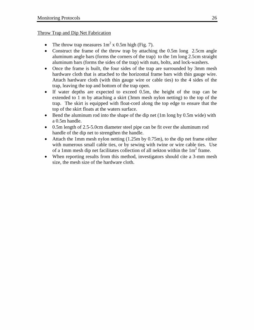
Throw Trap and Dip Net Fabrication
• The throw trap measures 1m2 x 0.5m high (Fig. 7). • Construct the frame of the throw trap by attaching the 0.5m long 2.5cm angle
aluminum angle bars (forms the corners of the trap) to the 1m long 2.5cm straight aluminum bars (forms the sides of the trap) with nuts, bolts, and lock-washers.
• Once the frame is built, the four sides of the trap are surrounded by 3mm mesh hardware cloth that is attached to the horizontal frame bars with thin gauge wire. Attach hardware cloth (with thin gauge wire or cable ties) to the 4 sides of the trap, leaving the top and bottom of the trap open.
• If water depths are expected to exceed 0.5m, the height of the trap can be extended to 1 m by attaching a skirt (3mm mesh nylon netting) to the top of the trap. The skirt is equipped with float-cord along the top edge to ensure that the top of the skirt floats at the waters surface.
• Bend the aluminum rod into the shape of the dip net (1m long by 0.5m wide) with a 0.5m handle.
• 0.5m length of 2.5-5.0cm diameter steel pipe can be fit over the aluminum rod handle of the dip net to strengthen the handle.
• Attach the 1mm mesh nylon netting (1.25m by 0.75m), to the dip net frame either with numerous small cable ties, or by sewing with twine or wire cable ties. Use of a 1mm mesh dip net facilitates collection of all nekton within the 1m2 frame.
• When reporting results from this method, investigators should cite a 3-mm mesh size, the mesh size of the hardware cloth.

Monitoring Protocols
27
Figure 7. 1m2 throw trap. The investigator is sweeping the trap with the 1m x 0.5m dip net. Note the skirt of 3mm nylon mesh net attached to the top of the trap for sampling in deeper water.

Monitoring Protocols
28
Materials for Sampling Nekton in Ponds
• 1m2 throw trap • small ruler (to measure nekton) • Map of pond station locations • Data sheet and pencils (Table 5) • Identification keys • Any other equipment necessary for taking environmental variables (e.g.
refractometer, oxygen probe, thermometer) Sampling Procedure for Nekton Using 1m2 Throw Trap
• Nekton sampling should occur at the same relative tide stage. • Sampling salt marsh ponds should occur only after the marsh surface is drained of
tidal water. We generally begin sampling in seaward habitats where the marsh surface drains first, and then proceed to landward areas following the tidal prism. This method ensures that samples are collected at similar water depths throughout the marsh, and is thus one way to control for the effects of tide stage.
• Samples are collected by approaching to within 4 to 5m of a marked station with the throw trap. Approach the station quietly so as not to not disturb or startle the nekton. Only the person throwing the throw trap should approach the station, all others should remain at a distance (>10m) from the station to avoid startling the nekton. Pond stations are approached by crouching low and walking over the marsh surface, then waiting about 2 minutes before throwing the trap.
• The trap is thrown into the water by tossing it from the hip like a giant Frisbee (Fig. 8). The trap is then quickly pushed into the sediment to prevent escape of nekton from under the trap. In order to minimize disturbance, replicates are never taken from the same station in a single sampling period.
• Once the sample is secured, nekton is removed by the large dip net. • The net is slid downward into the trap, flush against the side of the trap nearest
the researcher. The net is then moved across the trap with the forward edge of the net always remaining flush against the sediment until the opposite side of the trap is reached. In muddy sediments the dip net often goes through a thin layer of surface sediment, capturing buried nekton. The net is then moved upward out of the trap, again keeping the leading edge flush against the far wall of the trap.
• The dip net should be used from at least three sides of the trap because nekton may be hiding in the trap corners.
• The dip-netting procedure is repeated until three consecutive dips do not capture any animals or if the first four dips come up empty. At this point the trap is considered empty.
• Animals are processed as they are captured. All animals are identified to species in the field and immediately released at the same station.
• In each sample, up to fifteen individuals of every species are measured to the nearest mm for total length (from the tip of the snout to the tip of the caudal fin for fishes; from the tip of the rostrum to the tip of the telson for shrimp) or carapace width for crabs (the distance between the two furthest points across the

Monitoring Protocols
29
carapace). Generally, dominant fish species (i.e. the mummichog, Fundulus heteroclitus) is counted and measured as two categories, juveniles (<45mm) and adults (>45mm). Juveniles and adults can be entered on the data sheets under separate species (Table 5).
• Nekton may be identified using any number of guides that are specific to the Atlantic coast and New England regions, including Bigelow and Schroeder (1953), Gosner (1978), and Robins et al. (1986), Eddy and Underhill (1978).
• Individuals that are difficult to identify may be humanely sacrificed by a strong blow to the head, preserved in 70% ethanol, and returned to the laboratory for identification.
• Any associated environmental variables should be measured at this time (see section entitled “Other Environmental Variables Monitored During Nekton Sampling”).

Monitoring Protocols
30
Figure 8. Sampling technique for 1m2 throw trap. The trap is tossed like a frisbee into the pond that is being sampled.

Monitoring Protocols
31
Table 5. Sample nekton throw trap field data sheet.
THROW TRAP DATA SHEET
SITE:_________________________ DATE: ____________________ TIME:__________ STATION #:___________ SAMPLING CREW: _________________________ GPS Coordinates: N__________________________ E_____________________________ Water temp: __________ Salinity: __________ DO: ___________ Water Depth: ____________ Tide (circle one): Flood Ebb Vegetation (circle one): Yes No Vegetation Species #2 _________________ Veg. % Cover: <1% 1-5% 5-25% 50-75% >75%
NEKTON SPECIES & MEASUREMENTS
SPECIES #1 _________________________ Total # of individuals: ________________
Talley (include measured fish): ____________________________________________________________
LENGTHS: ___________________________________________________________________________ (15)
SPECIES #2 _________________________ Total # of individuals: ________________
Talley (include measured fish): ____________________________________________________________
LENGTHS: ___________________________________________________________________________ (15)
SPECIES #3 _________________________ Total # of individuals: ________________
Talley (include measured fish): ____________________________________________________________
LENGTHS: ___________________________________________________________________________ (15)
SPECIES #4 _________________________ Total # of individuals: ________________
Talley (include measured fish): ____________________________________________________________
LENGTHS: ___________________________________________________________________________ (15)
SPECIES #5 _________________________ Total # of individuals: ________________
Talley (include measured fish): ____________________________________________________________
LENGTHS: ___________________________________________________________________________ (15)

Monitoring Protocols
32
NEKTON SAMPLING IN DITCHES and SMALLER TIDAL CREEKS
SUMMARY
Common features on salt marshes are grid ditches that were created for mosquito control purposes in the 1940’s. These ditches vary in width, (usually 45cm and 100cm in wide) and on some marshes, especially those in the southern New England, are the only water habitat within the marsh. The throw trap is not a good sampling gear for the grid ditch habitat, as the trap is too large. Even smaller versions of a throw trap would not sample these areas as the trap would have to land precisely in the ditch in order to enclose the nekton. This protocol outlines an enclosure sampling gear, the ditch net, that we have designed to sample these narrow tidal channels. The center body of the net lines the sides and bottom of 1 linear meter (approximately) of ditch. There are two doors on the open ends of the net, which when pulled, rise up to close off the ends of the net, enclosing an area of water that is 1m long and as wide as the ditch. This sampling gear is designed to sample mosquito ditches and smaller tidal creeks up to 1m wide and 1m deep. There should be two daytime sampling efforts per year; one in early summer (June-July) and another in late summer-early fall (August-October), unless there are species or processes unique to other seasons that are of interest. The number of ditch net samples required depends on the habitat under examination, but initially we recommend at least 10 samples should be collected from each sampled habitat during each sample period. Materials for Identifying Ditch Station Locations
• Oak stakes to mark station locations • Mallet to pound stakes into ground • Black permanent markers to mark transect and plot number on stakes • Colored flagging (optional) to tie to oak stakes • Random number table (to determine specific station location along ditches) • Aerial photos of study sites • Map of study site showing boundaries of study areas and approximate location of
ditches Nekton Ditch Station Location Procedure All sampling stations should be randomly selected prior to monitoring. This is best accomplished by obtaining an aerial photograph of the study location to identify the ditches and smaller tidal creeks (<1m wide).
• Estimate length of ditch. • Choose a random number (from a random number table) between zero and the
total ditch length.

Monitoring Protocols
33
• Locate station location at the random number and mark with a 1m oak stake and colored flagging. For example, if the ditch is 120m long and the random number is 33, the station would be located at 33m along the ditch.
• Label stake with ditch net station ID. The naming convention for ditch stations is “D” for ditch and the station number, one through the total number of stations sampled in that area (e.g. D1, D2, etc.).
• Establish at least 10 ditch net stations per study area. • Generally, only one station is located per ditch. • If there are few ditches, more than one station can be located on the same ditch,
but the station should be at least 20m apart. • Record geographic coordinates (UTM, latitude/longitude) of all station locations
using a sub-meter accurate GPS unit.
Materials for Ditch Net Construction (for 1 net)
• NYLON netting (24lb test), 1/8in mesh, at least 1m deep. Each net takes 5 meters of netting – a 1m X 3m section for the center of the net (sides & bottom) and two 1m X 1m sections the doors
• 20m of nylon rope, 3/16in diameter. Each net takes 20m of line – four 4m lengths for rip cords and four 1m lengths for runner lines of the doors
• 5m of leadcore line; m for the top of each door (total 2m) and 3m for the floor of the net
• 4 eye-hooks with 1in eyes • 4 oak stakes – 1.5 to 2m long, 2.5cm square • Staple gun and 3/8 in stainless steel staples • D-ring hand pliers and 9/16 in C-ring fasteners • 25 to 30 plastic rings or rubber O rings, approximately 2.5cm diameter
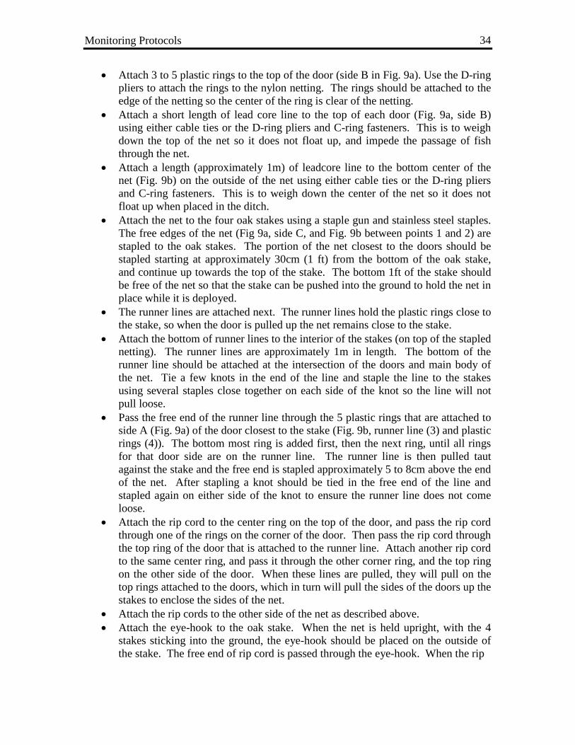
Ditch Net Fabrication
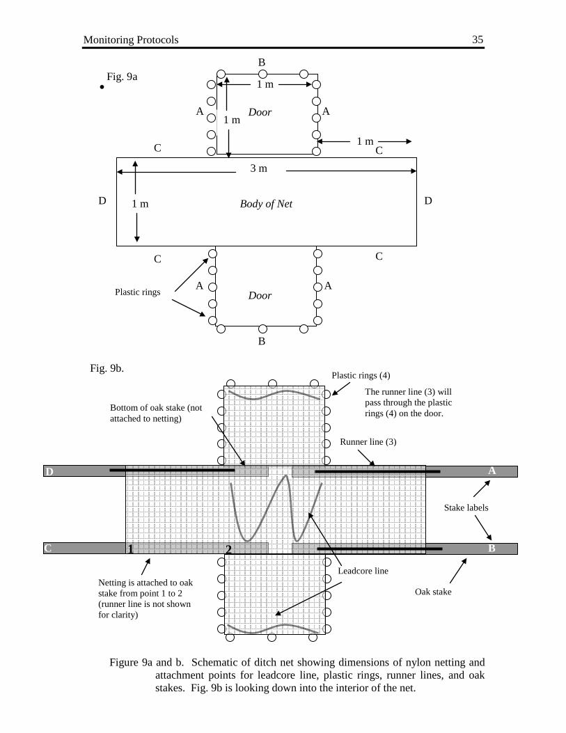
• Cut a 1m by 3m section of the nylon netting for the center of the net. • Cut two 1m by 1m sections of nylon netting for the doors of the net. • Attach the doors of the net to the center section. The doors should be centered on
the main body of the net along the 3m length (Fig 9a). To attach the doors take a 1m length of leadcore line and wrap the nylon netting from the leading edge of the door and the center 1m middle section of the net body around the leadcore and fasten the two pieces of nylon netting to the leadcore line with the D-ring pliers and 9/16 in C-ring fasteners.
• Attach 5 to 7 nylon rings or rubber O-rings to sides of the doors (side A in Fig 9a). Use the D-ring pliers to attach the rings to the nylon netting. The rings should be attached to the edge of the netting so the center of the ring is clear of the netting. The draw cord that pulls the doors up passes through these rings.
Monitoring Protocols
34
• Attach 3 to 5 plastic rings to the top of the door (side B in Fig. 9a). Use the D-ring pliers to attach the rings to the nylon netting. The rings should be attached to the edge of the netting so the center of the ring is clear of the netting.
• Attach a short length of lead core line to the top of each door (Fig. 9a, side B) using either cable ties or the D-ring pliers and C-ring fasteners. This is to weigh down the top of the net so it does not float up, and impede the passage of fish through the net.
• Attach a length (approximately 1m) of leadcore line to the bottom center of the net (Fig. 9b) on the outside of the net using either cable ties or the D-ring pliers and C-ring fasteners. This is to weigh down the center of the net so it does not float up when placed in the ditch.
• Attach the net to the four oak stakes using a staple gun and stainless steel staples. The free edges of the net (Fig 9a, side C, and Fig. 9b between points 1 and 2) are stapled to the oak stakes. The portion of the net closest to the doors should be stapled starting at approximately 30cm (1 ft) from the bottom of the oak stake, and continue up towards the top of the stake. The bottom 1ft of the stake should be free of the net so that the stake can be pushed into the ground to hold the net in place while it is deployed.
• The runner lines are attached next. The runner lines hold the plastic rings close to the stake, so when the door is pulled up the net remains close to the stake.
• Attach the bottom of runner lines to the interior of the stakes (on top of the stapled netting). The runner lines are approximately 1m in length. The bottom of the runner line should be attached at the intersection of the doors and main body of the net. Tie a few knots in the end of the line and staple the line to the stakes using several staples close together on each side of the knot so the line will not pull loose.
• Pass the free end of the runner line through the 5 plastic rings that are attached to side A (Fig. 9a) of the door closest to the stake (Fig. 9b, runner line (3) and plastic rings (4)). The bottom most ring is added first, then the next ring, until all rings for that door side are on the runner line. The runner line is then pulled taut against the stake and the free end is stapled approximately 5 to 8cm above the end of the net. After stapling a knot should be tied in the free end of the line and stapled again on either side of the knot to ensure the runner line does not come loose.
• Attach the rip cord to the center ring on the top of the door, and pass the rip cord through one of the rings on the corner of the door. Then pass the rip cord through the top ring of the door that is attached to the runner line. Attach another rip cord to the same center ring, and pass it through the other corner ring, and the top ring on the other side of the door. When these lines are pulled, they will pull on the top rings attached to the doors, which in turn will pull the sides of the doors up the stakes to enclose the sides of the net.
• Attach the rip cords to the other side of the net as described above. • Attach the eye-hook to the oak stake. When the net is held upright, with the 4
stakes sticking into the ground, the eye-hook should be placed on the outside of the stake. The free end of rip cord is passed through the eye-hook. When the rip
Monitoring Protocols
35
•
1 2
3 m
1 m
1 m Door
Body of Net
1 m
1 m
Door
A A
A A
B
B
C
C
C
C
D D
Figure 9a and b. Schematic of ditch net showing dimensions of nylon netting and attachment points for leadcore line, plastic rings, runner lines, and oak stakes. Fig. 9b is looking down into the interior of the net.
Fig. 9a
Plastic rings
Runner line (3)
Netting is attached to oak stake from point 1 to 2 (runner line is not shown for clarity)
Bottom of oak stake (not attached to netting)
Fig. 9b.
Oak stake
The runner line (3) will pass through the plastic rings (4) on the door.
Plastic rings (4)
Leadcore line
A
B
D
C
Stake labels

Monitoring Protocols
36
is pulled the line should pass easily through the eye-hook, so the doors are pulled up smoothly.
• Label the stakes. We usually label the stakes A, B, C, and D. Be sure to label each net exactly the same. The labels are used to set the net correctly in the ditch and to measure the distance between the stakes in order to determine the area of the water that the net was fishing (refer to data sheet). For example, stakes A and B are place on one side of the ditch and stakes C and D are place on the opposite side of the ditch (Fig. 9b).
• Test each net to be sure that the rip cords pull up the doors smoothly and quickly.
Materials for Sampling Nekton in Ditches
• Ditch nets • small ruler (to measure nekton) • meter stick (to measure net, creek and water depths) • Map of ditch station locations • Data sheet and pencils (Table 6) • Identification keys • Any other equipment necessary for taking environmental variables (e.g.
refractometer, oxygen probe, thermometer) Sampling Procedure for Nekton Ditch Net
• Nekton sampling in ditches should occur at the same relative tide stage. Sampling salt marsh ditches should occur only after the marsh surface is drained of tidal water. Sampling should occur on a high slack or ebb tide, when the marsh surface has drained.
• Nets are placed at the station locations in the ditches at least 30min before sampling. This usually means that the nets are placed at flood or slack tide.
• Set up a ditch net usually requires 2 people, each standing on opposite sides of the ditch. One person will take stakes labeled “A” and “B” and place the stakes into the bottom of the ditch close to the side of the ditch. The other person will take stakes labeled “C” and “D” and place them on the opposite side of the ditch. The net should be stretched tight between stakes “A” and “B” and stakes “C” and “D” so that approximately a 1m section of ditch is sampled. (Fig 10a).
• The rip cords should be pulled to make sure that the lines are not fouled and that the doors will pull up smoothly and quickly.
• Push the doors and the center of the net down into the bottom of the ditch with the meter stick. Make sure that the net lays down on the bottom of the ditch, so that fish passage through the net is not impeded.
• Measure the distance between all the stakes (e.g. “A” to “B”, “B” to “C”, “C” to “D”, and “D” to “A”) and the diagonal distance between stakes “A” and “C” and record these on the datasheet (Table 6). These distances are measured when the

Monitoring Protocols
37
net is placed in the ditch and are necessary to calculate the area of water that is sampled.
• Lay the rip cords out on the marsh surface as far from the net as possible without pulling on the doors.
• Note the time that the net is deployed on the data sheet. • Ditch nets should not be sampled until they have been deployed for at least
30min. This time period is necessary to minimize any disturbance to nekton caused by placing the net in the ditch.
• At high slack or ebb tide, the ditch nets are pulled. Two people are required to pull the ditch nets. The nets are quietly approached from opposite sides of the ditch, one person on each side. Upon reaching the rip cords, each person kneels and waits quietly for approximately 2min. The rip cords should not be handled during this time, as the vibrations on the cords can be transmitted to the stakes and possibly disturb nekton that are in the net. At a pre-determined signal, both people quickly pull on the rip cords and run towards the net. The doors of the net will pull up, enclosing nekton within the net (Fig. 10b and 10c).
• The net is then quickly lifted out of the ditch and onto the marsh surface. The best way to do this is to have both people pull the stakes out simultaneously (while still maintaining pressure on the rip cords). All four stakes are then handed to one person who will lift the net out of the ditch and onto the marsh surface. It is important to quickly pull the stakes and net out of the ditch, since this creates a bag of netting in the center of the net where the fish are trapped.
• The net is then laid out on the marsh surface and the nekton are identified, counted, and measured.
• The collection time should be recorded. • In each sample, up to fifteen individuals of every species are measured to the
nearest mm for total length (from the tip of the snout to the tip of the caudal fin for fishes; from the tip of the rostrum to the tip of the telson for shrimp) or carapace width for crabs (the distance between the two furthest points across the carapace). Generally, dominant fish species (i.e. mummichog, Fundulus heteroclitus) is counted and measured as two categories, juveniles (<45mm) and adults (>45mm). Juveniles and adults can be entered on the data sheets under separate species.
• Nekton may be identified using any number of guides that are specific to the Atlantic coast and New England regions, including Bigelow and Schroeder (1953), Gosner (1978), and Robins et al. (1986), Eddy and Underhill (1978).
• Any associated environmental variables should be measured at this time (see section entitled “Other Environmental Variables Monitored During Nekton Sampling”).

Monitoring Protocols
38
Calculating the Area of a Ditch Net
• The area of a ditch net is calculated as the sum of two irregular triangles. • The areas of the 2 irregular triangles are calculated from the 5 distances measured
in the field. • The formula for an irregular triangle is:
)])()((*[ csbsass −−−
Where: 2
)( cbas ++=
• For example, a net with the following dimensions: Where:
A to B = 81cm B to C = 73cm C to D = 71cm D to A = 76cm
A to C (diagonal) = 109cm
s for Triangle 1: 2
)1097381( ++=s = 131.5
The area of Triangle 1: )]1095.131)(735.131)(815.131(*5.131[ −−− = 2684.9cm2
s for Triangle 2: 2
)1097671( ++=s = 128
The area of Triangle 2: )]109128)(76128)(71128(*128[ −−− = 2956.5cm2
The total area of the net would be: 2956.5cm2 + 2684.9cm2 = 5641.4cm2 or 0.56m2
b
c
a
a A B
C D
b c 1
2

Monitoring Protocols
39
Figure 10a-c. Photos of ditch net in the field showing correct deployment (Fig 10a), doors being pulled up (Fig. 10b), and the net once the doors have been pulled (Fig 10c).
Fig 10a
Fig 10b
Fig 10c

Monitoring Protocols
40
Table 6. Sample nekton ditch net field data sheet.
Nekton Ditch Sampler Data Sheet
SITE:_________________________ DATE: ____________________ STATION #:___________ SAMPLING CREW: _______________________ GPS Coordinates: N____________________________ E________________________ Habitat Type: Tidal Creek (TC) Open Ditch (OD) Plugged Ditch (PD) Deployment Time: ___________ Collection Time: _____________________ Net Distance Measurements: A to B:_______ B to C:_______ C to D: _______ D to A: _______ A to C (diagonal): _______ Water temp: __________ Salinity: __________ DO: ___________ Water Depth: ____________ Creek/Ditch Depth: ___________ Tide: Flood or Ebb
NEKTON SPECIES & MEASUREMENTS
SPECIES #1 _________________________ Total # of individuals: ________________
Talley (include measured fish): ____________________________________________________________
LENGTHS: ___________________________________________________________________________
SPECIES #2 _________________________ Total # of individuals: ________________
Talley (include measured fish): ____________________________________________________________
LENGTHS: ___________________________________________________________________________
SPECIES #3 _________________________ Total # of individuals: ________________
Talley (include measured fish): ____________________________________________________________
LENGTHS: ___________________________________________________________________________
SPECIES #4 _________________________ Total # of individuals: ________________
Talley (include measured fish): ____________________________________________________________
LENGTHS: ___________________________________________________________________________
SPECIES #5 _________________________ Total # of individuals: ________________
Talley (include measured fish): ____________________________________________________________
LENGTHS: ___________________________________________________________________________

Monitoring Protocols
41
BIRD SURVEYS
SUMMARY The bird guilds using salt marsh areas within Region 5 that may be affected by OMWM practices include: (1) cryptic marsh passerine species such as marsh wrens and salt marsh sparrows (Seaside, Coastal Plain, Swamp, and Sharp-tailed primarily) and non-passerine rails and bitterns; (2) conspicuous, large waterbirds such as waterfowl (ducks, geese, and swans), colonial species such as herons and egrets, gulls, terns, Black Skimmers, and Double-crested Cormorants; and (3) migrating and wintering shorebirds, including sandpipers, plovers, and relatives. Many of these species are of high priority in state and national bird conservation plans, Partners in Flight, and Region 5 FWS. These groups however require different survey methods. Because previous work on breeding salt marsh sparrows had begun in New England in 1998, the same protocol used then, developed by James Gibbs and Greg Shriver, SUNY-Syracuse, should continue at the northern refuges, Parker River and Rachel Carson NWRs. It is probably necessary to add points specifically in the OMWM study areas at these northern refuges, although usually only one point could fit into each treatment area (points have a 100m radius, and adjacent points must be 300 m apart, according to the Shriver protocol). At ALL refuges, starting in 2002 or 2003, the marsh sparrow surveys will be combined with those for the other bird groups. The surveys will be conducted both in the breeding and non-breeding seasons. Although the same fixed walking route (see details below) can be used as with the Group 2 and 3 species, the bird survey method varies somewhat. Methods: Group 1 Species:
• A trained observer should conduct the survey (see Training section below). If possible, having a second person as a recorder is desirable.
• The observer should maintain a slow pace following a flagged walking route, recording all passerine bird species (sparrows, wrens) seen (flushed or perched) or heard within a 25 m distance from the survey line.
• Detections that are visual (V) or auditory (A) should be recorded on the form. Auditory detections will be the most critical for a few of the marsh passerines as well as the rails and bitterns.
• For birds that flush, try to mentally record their new location to avoid double-counting individuals. This method will certainly underestimate Sharp-tailed Sparrows which are not vocal (except during periods after spring tides) and are non-territorial, however it should be more effective for Seaside and Swamp sparrows.
• Because the surveys will be conducted with the larger Group 2-3 species and will focus on low-tide periods, time of day will vary from morning to afternoon. (Again, this is not optimal for passerine surveys, but Seaside and Swamp sparrows are very vocal species in the breeding season).

Monitoring Protocols
42
• The order of visitation of the treatment and control areas should be varied each survey, so that no systematic time bias results; e.g., avoid going to only controls early, treatments late in the day.
Methods Groups 2 and 3 Species:
• A four-season survey design is desired. • At least 5 replicates for each season should be performed: Spring/breeding (May
10 – June 30), late Summer (July 20 – September 10), late fall (October 15 – December 10) and Winter (January 10 – March 10).
• For these groups, detailed maps of the study area (2 + ha plot) should be used to set up the survey route and discrete habitats (creek segment, panne, pond, OMWM ditch) should be marked.
• Later, data analyses will require converting bird estimates to densities using both water (or basin) area and total plot area.
• Surveys should be timed to coincide with falling (>3hrs past high tide) or low tide (2hr before to 2hr after low), during daylight hours between 1hr after sunrise to 1 h before sunset.
• A fixed point should be established along one side of the area, preferably elevated (blind or scaffolding), that will allow the observer to use a spotting scope (15-20 X) and scan the entire area.
• All birds seen or heard are recorded, including those flying over the area that are feeding in the area, not simply transiting over (includes northern harriers, tree swallows, peregrine falcon, etc.).
• Birds should be assigned to one of the habitats listed on the form. Water bodies without daily tidal influence are considered "nontidal,"
therefore plugged ditches would be nontidal. Unplugged ditches would be tidal. For the aerial feeders, the habitat should be "Air".
• It is easiest to cover different sectors of the plot in sequence (e.g., N to S) recording all species by habitat use.
• We recommend using tick marks in the field form block as sectors accumulate, then in each block, at the end of the survey (10min minimum to 15min maximum) total the ticks and circle the number (see field sheet example).
• The notation of "FP" should be used in the left-hand column for all birds detected (A or V) from the fixed point observation.
• At the end of the 15min, draw a line across the form under the line for the last species entered. This will prevent confusion between entries for the FP and the walking route parts of the survey.
• A walking route (WR) transect marked with wire flagging (different colors than those used for marking nekton stations and vegetation plots) should be followed to survey each water body, panne, ditch, or creek as potential habitat.
• At regular intervals along the WR, GPS locations should be recorded in case flags disappear.

Monitoring Protocols
43
• Water levels in ditches and ponds should be crudely estimated and averaged for the entire plot area, not each water body (scores of 1-4, where 1=<25% basin full, 2=25-50% etc.); this will allow more refined analyses of bird densities.
• The observer should maintain a slow, steady pace, but should stop at larger water bodies to record, or at long tidal ditches to inspect for rails, and cryptic birds with binoculars.
• The observer should record the number of individuals of each species within a given habitat, with careful attention noted of species movements; i.e., avoid double counting birds that flush ahead and land in the next location visited.
• As before, we recommend using tick marks in each habitat block as one walks along, then totaling and circling the number in each habitat block after the transect is completed.
• Because the surveys are conducted around low tides, most birds are expected to be using ditches, creek banks, or pools/pannes.
• Also recorded should be those species that feed aerially (Habitat = Air), such as harriers, terns, falcons. (NOTE: We no longer recommend recording behavior during the surveys).
• The data should be recorded on field forms (Table 7) and if possible entered the same day in electronic format.
• A second individual should cross check the field forms and electronic database. The data should be maintained in a Microsoft Access database format that is being developed by PWRC personnel in consultation with other personnel involved with the OMWM project.
Training
• Observers need to be able to identify all species of waterbirds and marsh birds by sight and sound. If necessary, they may need to listen to tape recordings of certain species (rails, sparrows) or may require field reinforcement with an expert. Tapes can be provided by the USGS Patuxent Wildlife Research Center if necessary.
• Ideally, at the beginning of each refuge study, a local expert should be used to conduct a series of 20-30 point counts (radius 25m) at marsh pannes, tidal creeks, impoundments, and emergent marsh plots. Accompanying the expert should be the refuge biologist and field technicians expected to conduct the bird surveys.
• They should record on field forms all the birds seen or heard during 10min point counts, keeping records independently and not talking during the sessions.
• After the sessions, a tally of total species and numbers should be compared among the observers.
• A "qualified" field observer must have identified > 90% of the total species correctly, and > 80% of the total numbers of individuals compared to the "expert."
• If not, that individual should receive more training and be retested, or not used. • We prefer this method to the much more time-consuming alternative of the
double-observer method where two observers are required on every survey and where a rigorous data collection protocol is required using primary and secondary observers.

Monitoring Protocols
44
• We strongly encourage that data collection for birds be conducted by the same observer at all the sites and that the same individuals be used between years to reduce observer variability, a major source of variation.
• Observers should be reinforced using markers at 10, 20, 25, …up to 50m distances so that they may accurately determine bird detections within 25m of the transect.
• Stakes should be set out at these fixed intervals in one field site. • During training, objects can be placed at varying distances for observers to
estimate. After estimating each distance, they are then told the actual distance, and the two distances recorded for side by side comparison.
• If the observer can consistently (> 90% of occurrences) estimate within 5 m of the 20-30 distances, he/she should be considered qualified.
Instructions for Filling Out Bird Survey Field Data Sheet These instructions are to be used for the OMWM waterbird data surveys. For continuation of the special marsh sparrow surveys at Rachel Carson and Parker River, Greg Shriver has provided the protocol for those, begun in 1999, and data for New England is being compiled by Greg Shriver.
OMWM WATERBIRD DATA: We have set up the field data forms in a manner that will be most efficient when entering into Microsoft Access. We plan on creating a data entry form in Access that will look very much like your field datasheets. Many of the fields on the Access data entry form will contain bound dropdown lists (for example, when you enter your bird species codes, there will be a set list that you must choose from) and automated calculations (total survey minutes will be calculated; bird totals will be summed across the habitat types and compared with your bird totals as a data check). Migration from the field datasheets to electronic form (Access) will be done at each refuge, and then forwarded to Mike Erwin’s group. TOP SECTION OF OMWM DATA FORM – Survey Description
• Refuge Name and Site Code: This is a combination of Refuge Code and Site Code. For example, Prime Hook Petersfield Treatment would be PHPT. Refer to Table 8 in the section entitled “Data Headers for Spreadsheets” for site codes.
• Date: two digit month and day, four digit year (e.g. 05/24/2001) • Observer: Use 3 initials. • Time: First conduct a Fixed Point (FP) survey at each unit where one vantage
point can cover the entire unit (elevated if possible). We decided to allow a 10-15 min window depending on numbers of birds and location. Do not exceed 15min. Time of day is not being standardized, but tide is. Use military time (i.e., 1:00 pm = 1300h). For walking surveys, try to stay within about 30 minutes. This will vary among survey units, but keep a slow, steady pace. The emphasis is on WATERBIRDS using ditches and waterbodies; other birds using marsh grasses

Monitoring Protocols
45
are to be recorded within 25m of the transect. Total survey times will be calculated by Access, based on the times that you enter in these fields.
• Time of Low Tide: Record the predicted time of low tide. Of course, factors may differ for each survey, depending on local conditions (wind, etc.). It is beneficial to note water levels on the main data form (Water Level column, second from the right edge of the form) at each waterbody surveyed (see Water Level below).
• Temperature: in degree F. • Wind speed: Check with nearest weather station, USCG, or military airport if
possible. Windspeed codes are listed on the datasheet: L(<5mph), M(6-12mph), S(>12mph).
MAIN SECTION OF OMWM DATA SHEET – Bird Data
• Survey type: Use abbreviations FP for Fixed Point and WR for Walking Route. When transitioning from conducting the Fixed Point to the Walking Route, draw a line sectioning off all FP data, and below the line write WR to start the WR section of data.
• Species: On your field datasheets, you may record the bird species in whatever way is best for you, although we recommend using the ABA 4-letter codes. When the data is entered in Access, a drop down list containing 4 letter codes and the species common name will be provided in this field so that all refuges will be using the same 4-letter codes. Abbreviation conventions are as follows: For common names with one word, take the first 4 letters, example: Dunlin = DUNL; common names with 2 words, take the first 2 letters from each word, example: Greater Yellowlegs = GRYE; For multiple species confusion, use the following conventions: For small unidentified sandpipers (the Least, Semipalmated, Western complex), use “PEEP”; for small terns (Forster’s or Common), use TERN, for unidentified dowitchers, use DOWI; for Greater or Lesser Yellowlegs, use YELL; for unidentified sparrow, use SPAR; for unidentified (usually immature) gulls, use GULL.
• Total Number of Birds: Tally this up at the end of the session. We suggest using tick marks in pencil as you count birds by species in each habitat type. After the survey is complete, add up the ticks in each cell, write the total in the cell, and circle it. The sum of all cells in a row is what you should write in the Total Number of Birds Column. We will use this column as a data check (it will be compared with a sum that Access calculates for each row).
• Habitat types: Self explanatory. To avoid double counting of individuals, record individuals in the first habitat that they were seen in ONLY (if a dunlin moves from a tidal pond to a ditch, record it in the tidal pond only). For analysis, we will create GIS layers and each habitat type will be measured for area. When analyses are underway, we will convert total numbers of birds by habitat type into density values. For birds seen in the air, only list species that are aerially feeding or hunting, not those obviously flying over. For example, you may list a northern harrier that is hovering.

Monitoring Protocols
46
• A or V: Record whether a bird was observed audially or visually. You don’t need to do this for the waterbirds, but please be sure to distinguish for the sparrows and secretive species such as rails and bitterns.
• Water Level: Note water levels in each waterbody (ditch, tidal pool, panne, etc.) using the codes provided on the sheet (1=25% full, 2=25-50%, etc.).
• Notes: Record any anomalies such as disturbances, use of heavy equipment, etc. Because the cell is pretty small, you might have to write over a couple of cells; be sure to demarcate which record the note refers to.
PAGE 2 - MAIN SECTION OF OMWM DATA SHEET – Bird Data Use this if you fill up the first sheet. Be sure to fill in the page number and the total number of pages for that survey in the top right corner (e.g., page 2 of 2).
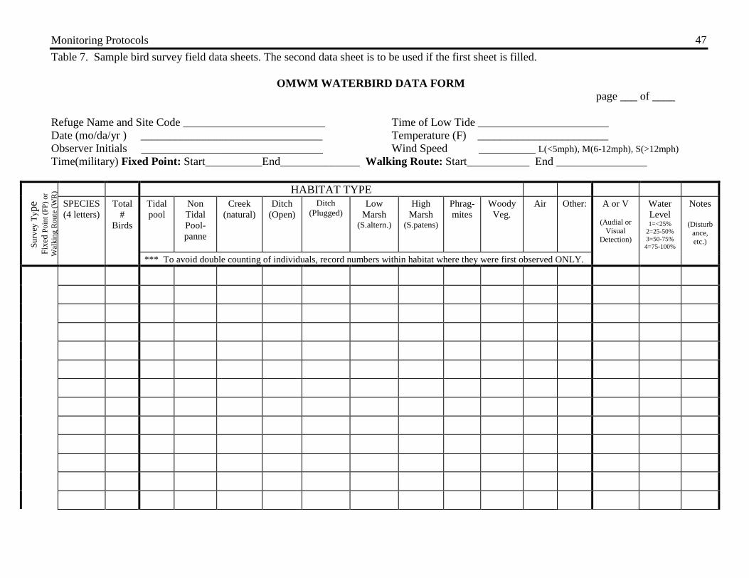
Monitoring Protocols
47 Table 7. Sample bird survey field data sheets. The second data sheet is to be used if the first sheet is filled.
OMWM WATERBIRD DATA FORM page ___ of ____
Refuge Name and Site Code _________________________ Time of Low Tide _______________________ Date (mo/da/yr ) ________________________________ Temperature (F) _______________________ Observer Initials ________________________________ Wind Speed __________ L(<5mph), M(6-12mph), S(>12mph) Time(military) Fixed Point: Start__________End______________ Walking Route: Start___________ End ________________
Surv
ey T
ype
Fi
xed
Poin
t (FP
) or
Wal
king
Rou
te (W
R) HABITAT TYPE
SPECIES (4 letters)
Total #
Birds
Tidal pool
Non Tidal Pool- panne
Creek (natural)
Ditch (Open)
Ditch (Plugged)
Low Marsh
(S.altern.)
High Marsh
(S.patens)
Phrag- mites
Woody Veg.
Air Other: A or V
(Audial or Visual
Detection)
Water Level 1=<25%
2=25-50% 3=50-75%
4=75-100%
Notes
(Disturbance, etc.)
*** To avoid double counting of individuals, record numbers within habitat where they were first observed ONLY.

Monitoring Protocols
48 Table 7. continued.
OMWM WATERBIRD DATA FORM Page ___ of ____
Refuge Name and Site Code __________________ Date (mo/da/yr ) _________________________ Temp.(F)__________
Surv
ey T
ype
Fi
xed
Poin
t (FP
) or
Wal
king
Rou
te (W
R) HABITAT TYPE
SPECIES (4 letters)
Total #
Birds
Tidal pool
Non Tidal Pool- panne
Creek (natural)
Ditch (Open)
Ditch (Plugged)
Low Marsh
(S.altern.)
High Marsh
(S.patens)
Phrag- mites
Woody Veg.
Air Other: A or V
(Audial or Visual
Detection)
Water Level 1=<25%
2=25-50% 3=50-75%
4=75-100%
Notes
(Disturbance, etc.)
*** To avoid double counting of individuals, record numbers within habitat where they were first observed ONLY.

Monitoring Protocols
49
OTHER ENVIRONMENTAL VARIABLES MONITORED DURING NEKTON SAMPLING
Once nekton is removed from a trap or ditch net sample, environmental variables can be measured. Measures of water temperature, salinity, water depth, and plant cover are essential environmental data to collect in conjunction with each throw trap and ditch net sample. Some investigators may elect to also collect other variables. Sediment composition (e.g. grain sizes and organic content) can be measured by extracting sediment cores and then processing according to Dean (1974). This information helps describe the habitat available to the nekton. Other variables such as creek width, creek order (e.g., 1st order, 2nd order), pond size, adjacent shoreline type, distance of seagrass bed to shoreline, are easy measures and can enhance interpretation of the nekton data. The following water quality measurements should be taken from an area of the pond or ditch that has not been disturbed (e.g. sediment re-suspension) from the throw trap or ditch net activity.
• Water temperature, to the nearest degree C, is measured using a stick thermometer or temperature probe.
• Salinity is measured, to the nearest part per thousand, using either a refractometer or water quality probe.
• Dissolved oxygen is measured using a dissolved oxygen probe. • Water depth within the trap is measured to the nearest cm using a meter stick.
Alternatively, the sides of the trap can be marked off in centimeters and readings taken directly from the trap. The trap is often located on an uneven bottom, and thus, depth should be measured near each corner of the trap to obtain a mean depth value. Water depth is a simple measure and is useful for documenting changes in water depth over time. When monitoring restoration sites, where hydrology has been altered, this is a particularly important measure.
• Water depth in the ditch is measured after the net is removed from the ditch. The depth of the ditch is also measured.
• If macroalgae, marsh grass, or eelgrass are present within the trap, cover and species composition should be quantified. Prior to dip netting for nekton, the percent cover of each plant species should be visually estimated according to the following cover class categories (<1% cover, 1-5%, 5-25%, 25-50%, 50-75%, >75%). These data provide a measure of the complexity of habitat available to the estuarine nekton. If sampling in regions with turbid waters and the vegetation can not be seen, then vegetation should be quantified by a biomass technique after Raposa and Oviatt (2000).

Monitoring Protocols
50
DATA MANAGEMENT AND QUALITY ASSURANCE AND QUALITY CONTROL
Field data should be recorded in waterproof notebooks or on datasheets that are previously developed and printed on waterproof paper. Datasheets can be organized to the preference of individual researchers, but should include all information described previously in these protocols (e.g., study site, date, station identification, habitat, species name, total number of individuals captured by species, lengths, comments, and environmental parameters). Examples of sample datasheets are provided after each protocol.
• Be sure to write legibly on the datasheet. • Make sure that all sections of the data sheet are filled out before moving on to the
next sampling station. • If a variable cannot or was not measured (e.g. instrument failure, fish escaped)
explain on the data sheet for that station the reason for missing data. Record the reason/explanation in the field. Do not wait until you return to the office to record the reason or explanation.
• All field data should be transferred to digital format soon after sampling. Field data are easily incorporated into common spreadsheet programs that are designed for comprehensive data management.
• After the data are entered it is important to carefully check the data for typos and mis-entries to insure the data are correct and to maintain quality assurance and quality control of the data.
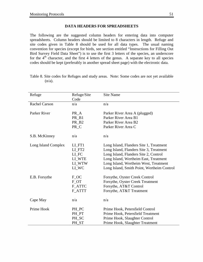
Monitoring Protocols
51
DATA HEADERS FOR SPREADSHEETS The following are the suggested column headers for entering data into computer spreadsheets. Column headers should be limited to 8 characters in length. Refuge and site codes given in Table 8 should be used for all data types. The usual naming convention for species (except for birds, see section entitled “Instructions for Filling Out Bird Survey Field Data Sheet”) is to use the first 3 letters of the species, an underscore for the 4th character, and the first 4 letters of the genus. A separate key to all species codes should be kept (preferably in another spread sheet page) with the electronic data. Table 8. Site codes for Refuges and study areas. Note: Some codes are not yet available
(n/a). Refuge Refuge/Site
Code Site Name
Rachel Carson n/a n/a Parker River PR_A Parker River Area A (plugged) PR_B1 Parker River Area B1 PR_B2 Parker River Area B2 PR_C Parker River Area C S.B. McKinney n/a n/a Long Island Complex LI_FT1 Long Island, Flanders Site 1, Treatment LI_FT2 Long Island, Flanders Site 3, Treatment LI_FC Long Island, Flanders Site 2, Control LI_WTE Long Island, Wertheim East, Treatment LI_WTW Long Island, Wertheim West, Treatment LI_WC Long Island, Smith Point, Wertheim Control E.B. Forsythe F_OC Forsythe, Oyster Creek Control F_OT Forsythe, Oyster Creek Treatment F_ATTC Forsythe, AT&T Control F_ATTT Forsythe, AT&T Treatment Cape May n/a n/a Prime Hook PH_PC Prime Hook, Petersfield Control PH_PT Prime Hook, Petersfield Treatment PH_SC Prime Hook, Slaughter Control PH_ST Prime Hook, Slaughter Treatment

Monitoring Protocols
52
Vegetation Data Headers All vegetation data for a refuge should be entered into a single spread sheet (i.e., do not use separate spreadsheets for each study area). The first and second columns identify the study area and the vegetation plot. The remaining columns are for the vegetation cover types that were observed at all study locations. It is helpful to first make a master list of all vegetation cover types that were observed within the Refuge study areas. Be sure to make a list of all vegetation cover type codes used and what they represent, so that others can interpret the codes. In each cell under the appropriate cover type for that plot, the total tally of “hits” would be entered. Table 9 shows an example of vegetation data entered for study sites at Prime Hook NWR for Slaughter Control (PH_SC) plot 2-40 and Petersfield Treatment (PH_PT), plot 1-100. At Slaughter Control, plot 2-40, S. alterniflora (Spa_alte) had 14 hits, S. patens (Spa_pate) had 45 hits, and bare ground had 3 hits, while at Petersfield Treatment, plot 1-100 had 50 hits of Phragmites australis (Phr_aust) and 15 hits on bare ground. Note that since all vegetation data for a refuge are entered into one spreadsheet, entries of “0” are entered if that species was not present at a particular plot. Only four species are shown in this example, however there will be more species for any particular Refuge. Table 9. Example of vegetation data entry. Study Site Plot ID Spa_alte Phr_aust Spa_pate Bare PH_SC 2-40 14 0 45 3 PH_PT 1-100 0 50 0 15

Monitoring Protocols
53
Water Table Level and Soil Salinity Data Headers Headers for data entry are shown in Table 10. Calculations can be done by hand and entered on the spreadsheet or can be entered as additional columns and the spreadsheet program can perform the calculation. For example, water table level is calculated as the top of the well measurement (A) minus the top of the well to the marsh surface (B). In the example below only the finished calculation is shown. Note that at Flanders treatment 1 (LI_FT1), stations 1-00 and 1-30, the water table depth was negative since the water table was below the surface, but at Wertheim control (LI_WC), station 1-60, there was water on the surface of the marsh and therefore the water table level was positive number. Missing data are entered as a “.” as at LI_WC, station 1-90. Table 10. Example of water table level and soil salinity data entry.
Mosquito Larvae Data Headers
Mosquito data headers are shown in Table 11. If the station is dry, then a missing value represented by “.” should be entered as the number of larvae observed. If water was present at the station, but no larvae were in the dipper, then “0” is entered for the number of larvae observed. For example, at Forsyth NWR’s Oyster Creek control site (F_OC), station 4-120, the station was dry and since there was no water present the number of larvae is entered as “.”. At the AT&T control site (station 1-40) water was present, but no larvae were in the dipper, so a “0” is entered. Missing values are entered for dry stations so as not to bias the counts by including habitats that are not appropriate for larval mosquitoes. If larvae were present, then enter “yes” or “no” in the appropriate species column indicating what species were found. This information will be entered after the larval samples have been identified. Be sure to keep information on species identification with the appropriate Mosquito Larvae Sampling Data Sheet. Only two mosquito species are shown for example purposes, it may be necessary to add more species columns. Note that codes for the amount of water volume in the dipper are entered instead of the actual volume.
Date Site Station # Water Table Depth
(cm) Soil Salinity
(ppt) Depth of Soil Salinity
(cm) 7/5/2001 LI_FT1 1-00 -2.8 25 15 7/5/2001 LI_FT1 1-30 -14.9 26 45 7/5/2001 LI_WC 1-60 3.7 20 15 7/5/2001 LI_WC 1-90 . . .

Monitoring Protocols
54
Nekton Data Headers Nekton data from both collection methods (throw trap and ditch net) are entered on the same spread sheet. Nekton data require two different spreadsheets since one data type deal with station information and the other with individual nekton (length) information. Table 12 illustrates the header information for example data from Parker River NWR. Note that the station ID also identifies the type of gear. For example, P1 stands for Pond 1 which is sampled with a throw trap, whereas D2 is a ditch net station which is sampled with a ditch net. Environmental variables such as water depth, creek depth, tide phase, water temperature, salinity, and DO are also entered. For throw trap samples, a missing value represented by “.” is entered for the creek depth since only the water depth of the pond is measured. Habitat type for ditch nets should be entered as TC (tidal creek), OD (open ditch) or PD (plugged ditch). Habitat type for throw traps is always “pond”. The area of the ditch net is from the measurements of the net (refer to section “Calculating the Area of a Ditch Net”). The area of throw trap samples is always 1m2. The remaining columns are for the nekton species that were observed at all study locations. The total count of individuals for that station is entered under each appropriate species. Note that species names are coded into an 8 letter code. Be sure to include a key to the codes with the database. If a nekton species was not present, represent that by a “.” not “0” as this will influence the final density calculation. Density is calculated as the sum total number of individuals per trap or ditch net divided by the area of the trap or net. The individual nekton (fish and decapods) data are entered in another spreadsheet. Headers for individual nekton data are shown in Table 13. In this database there is one “species” column and the species coded name is entered and the corresponding length of that fish is entered in the corresponding cell under “length”. Carapace width (for crabs) and total length (for shrimps) are also entered under the length. Note that Fundulus heteroclitus adults (Fun_hetA) and juveniles (Fun_hetJ) are given separate species codes. Be sure to include a key to the codes with the database. Bird Survey Data Headers An Access Database with drop down menus has been designed for bird survey data entry by Diann Prosser, USGS, Patuxent Wildlife Research Center. All refuges will receive a copy of this database for bird survey data entry.
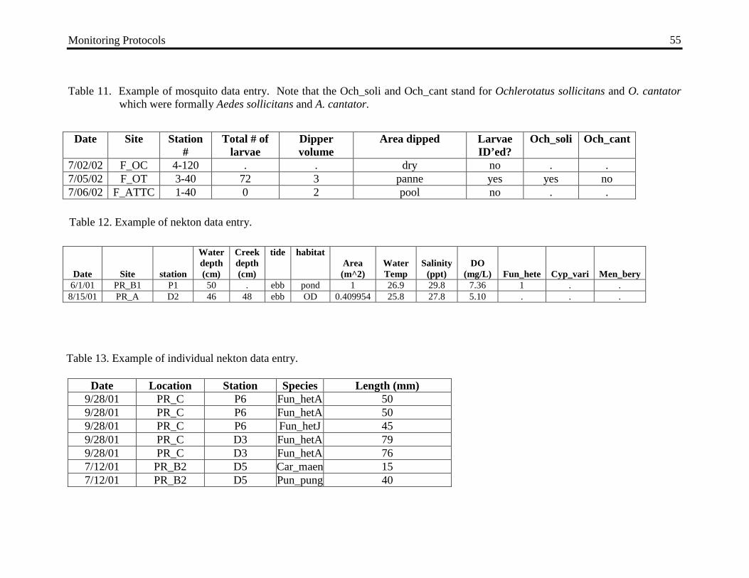
Monitoring Protocols
55
Table 11. Example of mosquito data entry. Note that the Och_soli and Och_cant stand for Ochlerotatus sollicitans and O. cantator which were formally Aedes sollicitans and A. cantator.
Date Site Station #
Total # of larvae
Dipper volume
Area dipped Larvae ID’ed?
Och_soli Och_cant
7/02/02 F_OC 4-120 . . dry no . . 7/05/02 F_OT 3-40 72 3 panne yes yes no 7/06/02 F_ATTC 1-40 0 2 pool no . .
Date Site station
Water depth (cm)
Creek depth (cm)
tide habitat Area (m^2)
Water Temp
Salinity (ppt)
DO (mg/L) Fun_hete Cyp_vari Men_bery
6/1/01 PR_B1 P1 50 . ebb pond 1 26.9 29.8 7.36 1 . . 8/15/01 PR_A D2 46 48 ebb OD 0.409954 25.8 27.8 5.10 . . .
Date Location Station Species Length (mm) 9/28/01 PR_C P6 Fun_hetA 50 9/28/01 PR_C P6 Fun_hetA 50 9/28/01 PR_C P6 Fun_hetJ 45 9/28/01 PR_C D3 Fun_hetA 79 9/28/01 PR_C D3 Fun_hetA 76 7/12/01 PR_B2 D5 Car_maen 15 7/12/01 PR_B2 D5 Pun_pung 40
Table 12. Example of nekton data entry.
Table 13. Example of individual nekton data entry.

Monitoring Protocols
56
LITERATURE CITED
Bigelow, H.B. and W.C. Schroeder. 1953. Fishes of the Gulf of Maine. U.S. Fish and Wildlife Service Bulletin 74:1-576.
Chambers, R.M., T.J. Mozdzer, and J.C. Ambrose. 1998. Effects of salinity and sulfide on the distribution of Phragmites australis and Spartina alterniflora in a tidal salt marsh. Aquatic Botany 62: 161-169.
Cline, J.D. 1969. Spectrophotometric determination of hydrogen sulfide in natural waters. Limnology and Oceanography 14: 454-458.
Dean, W.E., Jr. 1974. Determination of carbonate and organic matter in calcareous
sediments and sedimentary rocks by loss on ignition: comparison with other methods. Journal of Sedimentary Petrology 44:242-248.
Eddy, S. and J. C. Underhill. 1978. How to Know the Freshwater Fishes. Wm. C.
Brown Company Publishers, Dubugue, IA. ISBN# 0-697-04750-4. Gosner, K.L. 1978. A Field Guide to the Atlantic Seashore: Invertebrates and
Seaweeds of the Atlantic Coast from the Bay of Fundy to Cape Hatteras. Houghton Mifflin, Boston, MA. 329 p.
Howes, B.L., J.W.H. Dacey, and D.D. Goehringer. 1986. Factors controlling the growth form of Spartina alterniflora: feedbacks between above-ground production, sediment oxidation, nitrogen and salinity. Journal of Ecology 74: 881-898.
Koch, M.S., I.A. Mendelsshon, and K.L. McKee. 1990. Mechanism for the hydrogen-
sulfide-induced growth limitation in wetland macrophytes. Limnology and Oceanography 35: 399-408.
Portnoy, J.W., and A.E. Giblin. 1997. Effects of historic tidal restrictions on salt marsh
sediment chemistry. Biogeochemistry 36: 275-303. Raposa, K.B. and C.A. Oviatt. 2000. The influence of contiguous shoreline type,
distance from shore, and vegetation biomass on nekton community structure in eelgrass beds. Estuaries 23:46-55.
Raposa, K.B. and C.T. Roman. 2000. Monitoring nekton in shallow estuarine habitats.
Part of a series of monitoring protocols for the Long-term Coastal Ecosystem Monitoring Program at Cape Cod National Seashore. USGS Patuxent Wildlife Research Center, Coastal Research Field Station, University of Rhode Island, Narragansett, RI 02882
Raposa, K.B., and C.T. Roman. 2001. Seasonal habitat-use patterns of nekton in a tidal-
restricted and unrestricted New England salt marsh. Wetlands 21: 451-461.

Monitoring Protocols
57
Robins, C.R., G.C. Ray, J. Douglass, and R. Freund. 1986. A Field Guide to Atlantic
Coast Fishes of North America. Houghton Mifflin, Boston, MA. 354 p. Roman, C.T., M.J. James-Pirri, J. F. Heltshe. 2001. Monitoring Salt Marsh Vegetation:
Part of a series of monitoring protocols for the Long-term Coastal Ecosystem Monitoring Program at Cape Cod National Seashore. USGS Patuxent Wildlife Research Center, Coastal Research Field Station, University of Rhode Island, Narragansett, RI 02882

Monitoring Protocols
58
FIELD IDENTIFICATION RESOURCES General Vegetation Gleason, H. A. and A. Cronquist. 1991. Manual of Vascular Plants of Northeastern
United States and Adjacent Canada 2nd ed.The New York Botanical Garden, Bronx, NY. ISBN# 0-89327-365-1.
Holmgren, N. H. 1998. Illustrated Companion to Gleason and Cronquist's Manual: Illustrations of the Vascular Plants of Northeastern United States and Adjacent Canada. The New York Botanical Garden, Bronx, NY. ISBN# 0-89327-399-6.
Newcomb, Lawrence. 1977. Newcomb's Wildflower Guide. Little, Brown and Company, Boston, MA.
Regional Vegetation Gould, L. L., R. W. Enser, R. E. Champlin, and I. H. Stuckey. 1998. Vascular Flora of
Rhode Island. A list of native and naturalized plants Vol. 1. Rhode Island Natural History Society, Kingston, RI, The Biota of Rhode Island, ISBN# 1-887771-01-8.
Haines, A. and T. F. Vining. 1998. Flora of Maine a Manual for Identification of Native and Naturalized Vascular Plants of Maine. V. F. Thomas Co., Bar Harbor, ME. ISBN# 01-9664874-0-0.
McDonnell, M. J. 1979. The Flora of Plum Island Essex County, Massachusetts. New Hampshire Agricultural Experiment Station, University of New Hampshire, Durham, NH, Station Bulletin 513.
Niering, W. A. and R. S. Warren. 1980. Salt Marsh Plants of Connecticut. The Connecticut Arboretum, Connecticut College, New London, CT, Bulletin No. 25.
Phillips, C. E. 1978. Wildflowers of Delaware and the Eastern Shore. Delaware Nature Education Society, Hockessin, DE.
Silberhorn, G. M. 1982. Common Plants of the Mid-Atlantic Coast - A Field Guide. The Johns Hopkins University Press, Baltimore, MD. ISBN# 0-8018-2725-6.
Tiner, R. W. Jr. 1987. A Field Guide to Coastal Wetland Plants of the Northeastern United States. The University of Massachusetts Press, Amherst, MA. ISBN# 0-87023-537-0.
General Animal Eddy, S. and J. C. Underhill. 1978. How to Know the Freshwater Fishes. Wm. C.
Brown Company Publishers, Dubugue, IA. ISBN# 0-697-04750-4. Gosner, K. L. 1978. A Field Guide to the Atlantic Seashore. Houghton Mifflin
Company, Boston, MA. ISBN# 0-395-24379-3. Robins, C. R., and G. C. Ray. 1986. A Field Guide to the Atlantic Coast Fishes.
Houghton Mifflin Company, Boston, MA. ISBN# 0-395-39198-9.

Monitoring Protocols
59
Regional Animal Able, K.W. and M.P. Fahay. 1998. The First Year in the Life of Estuarine Fishes in the
Middle Atlantic Bight. Rutgers University Press, New Brunswick, NJ,. ISBN# 0-8135-2500-4.
Bigelow, H. B. and W. C. Schroeder. 1953. Fishes of the Gulf of Maine. Fishery Bulletin of the Fish and Wildlife Service, Vol. 53, United States Government Printing Office, Washington, D. C.
Raasch, M. S. 1997. Delaware's Freshwater and Brackish-Water Fishes. Delaware Nature Society, Dover, DE.
Whitworth, W.R. Freshwater Fishes of Connecticut. 1996. State Geological and Natural History Survey of Connecticut, Department of Environmental Protection. Second Ed., Bulletin114, Hartford, CT. ISBN# 0-942081-08-0. (DEP Maps and Publication Office, 79 Elm St., Hartford, CT 06106, 806-424-3555).
Weiss, H. M. 1997. Marine Animals of Southern New England and New York. State Geological and Natural History of Connecticut Department of Environmental Protection, Bulletin115, Hartford, CT. ISBN# 0-942081-06-4.

Monitoring Protocols
60
CONTACT INFORMATION Project Contacts
Mary-Jane (M.J.) James-Pirri Graduate School of Oceanography, University of Rhode Island Narragansett, RI 02882 Telephone: (401) 874-6617 Fax: (401) 874-6887 E-mail: [email protected] Charles Roman National Park Service Graduate School of Oceanography, University of Rhode Island Narragansett, RI 02882 Telephone: (401) 874-6886 (voice) Fax: (401) 874-6887 (fax) E-mail: [email protected] Susan Adamowicz Graduate School of Oceanography, University of Rhode Island Narragansett, RI 02882 Telephone: (401) 874-6617 Fax: (401) 874-6887 E-mail: [email protected] R. Michael Erwin USGS Patuxent Wildlife Research Center Clark Hall, Dept. of Environmental Sciences University of Virginia Charlottesville, VA 22903 Telephone: (434) 924-3207 Fax: (434) 982-2137 E-mail: [email protected] Diann (De) Prosser USGS – Patuxent Wildlife Research Center 11410 American Holly Drive Laurel, MD 20708-4015 Telephone: (301)-497-5914 E-mail: [email protected]

Monitoring Protocols
61
Refuge Contacts
Project Coordinator Janith Taylor Telephone: (603) 431-5581 Fax: (603) 431-6014 E-mail: [email protected]
E.B. Forsythe NWR Jorge Coppen E-mail: [email protected] Great Creek Road Oceanville, NJ 08231 Telephone: (609) 652-1665 Fax: (609) 652-1474 Long Island NWR Complex, Wertheim NWR Mark Maghini E-mail: [email protected] 360 Smith Road Shirley, NY 11967-0021 Telephone: (631)-286-0485 Fax: (631)-286-4003 Parker River NWR Deb Melvin & Mauve Taylor E-mail: [email protected] E-mail: [email protected] 261 Northern Boulevard Plum Island Newburyport, MA 01950-4315 Telephone: (978)-465-5753 Fax: (978)-465-2807 Prime Hook NWR Annabella (Annie) Larsen E-mail: [email protected] P.O. Box 195 Route 3 Milton, DE 19968 Telephone: (302) 684-8419 Fax: (302)-684-8504

Monitoring Protocols
62
Rachel Carson NWR Kate O’brien E-mail: [email protected] 321 Port Road Wells, ME 04090 Telephone: (207)-646-9226 Fax: (207)-646-6554 Stewart B. McKinney NWR Sara Williams E-mail: [email protected] P.O. Box 1030 Westbrook, Connecticut 06498-2513 Telephone: (860)-399-2513 Fax: (860)-399-2515