Nested sampling of isobaric phase space for the direct evaluation of the isothermal-isobaric partition function of atomic systemsBlake A. Wilson, Lev D. Gelb, and Steven O. Nielsen Citation: The Journal of Chemical Physics 143, 154108 (2015); doi: 10.1063/1.4933309 View online: http://dx.doi.org/10.1063/1.4933309 View Table of Contents: http://scitation.aip.org/content/aip/journal/jcp/143/15?ver=pdfcov Published by the AIP Publishing Articles you may be interested in Evaluation of the grand-canonical partition function using expanded Wang-Landau simulations. II. Adsorptionof atomic and molecular fluids in a porous material J. Chem. Phys. 136, 184108 (2012); 10.1063/1.4712025 Surface excess free energy of simple fluids confined in cylindrical pores by isothermal-isobaric Monte Carlo:Influence of pore size J. Chem. Phys. 126, 184701 (2007); 10.1063/1.2735582 Molecular dynamics in the isothermal-isobaric ensemble: The requirement of a “shell” molecule. I. Theory andphase-space analysis J. Chem. Phys. 123, 164101 (2005); 10.1063/1.2064512 Absolute entropy and free energy of fluids using the hypothetical scanning method. I. Calculation of transitionprobabilities from local grand canonical partition functions J. Chem. Phys. 119, 12084 (2003); 10.1063/1.1625919 Determination of equilibrium pitch of cholesteric phases by isobaric–isothermal Monte Carlo simulation J. Chem. Phys. 114, 8210 (2001); 10.1063/1.1365086

This article is copyrighted as indicated in the article. Reuse of AIP content is subject to the terms at: http://scitation.aip.org/termsconditions. Downloaded to IP:

129.110.242.59 On: Wed, 21 Oct 2015 16:10:28

THE JOURNAL OF CHEMICAL PHYSICS 143, 154108 (2015)

Nested sampling of isobaric phase space for the direct evaluationof the isothermal-isobaric partition function of atomic systems

Blake A. Wilson,1 Lev D. Gelb,2 and Steven O. Nielsen11Department of Chemistry, University of Texas at Dallas, Richardson, Texas 75080, USA2Department of Materials Science and Engineering, University of Texas at Dallas, Richardson,Texas 75080, USA

(Received 4 March 2015; accepted 5 October 2015; published online 21 October 2015)

Nested Sampling (NS) is a powerful athermal statistical mechanical sampling technique that directlycalculates the partition function, and hence gives access to all thermodynamic quantities in absoluteterms, including absolute free energies and absolute entropies. NS has been used predominately tocompute the canonical (NVT) partition function. Although NS has recently been used to obtain theisothermal-isobaric (NPT) partition function of the hard sphere model, a general approach to thecomputation of the NPT partition function has yet to be developed. Here, we describe an isobaricNS (IBNS) method which allows for the computation of the NPT partition function of any atomicsystem. We demonstrate IBNS on two finite Lennard-Jones systems and confirm the results throughcomparison to parallel tempering Monte Carlo. Temperature-entropy plots are constructed as wellas a simple pressure-temperature phase diagram for each system. We further demonstrate IBNS bycomputing part of the pressure-temperature phase diagram of a Lennard-Jones system under periodicboundary conditions. C 2015 AIP Publishing LLC. [http://dx.doi.org/10.1063/1.4933309]

I. INTRODUCTION

In the context of molecular simulation, the partitionfunction and consequently the absolute thermodynamic prop-erties used to be considered inaccessible.1 Metropolis2 styleMonte Carlo simulations provided a means to computethermodynamic averages without direct knowledge of thevalue of the partition function. Similarly, various free energymethods, such as free energy perturbation and thermodynamicintegration, have been developed to determine free energydifferences without direct access to the partition function.3

However, interest began to grow in the ability to compute thepartition function and the absolute thermodynamic propertiesin fields such as pure substance reference data4 and proteinfolding.5 Methods such as Wang-Landau, multicanonical, andhistogram reweighting have been developed in order to allowfor computation of the density of states6 (DOS) and conse-quently the partition function. However, most of these methodsstill struggle in the vicinity of phase transitions.3,7 A relativelynew athermal method called Nested Sampling (NS) provides asimple yet powerful way to compute partition functions whileeffortlessly handling phase transitions. Originally developedin the context of Bayesian computation by Skilling,8,9 NSwas designed to efficiently compute the evidence (partitionfunction) of high dimensional spaces where the bulk of theprobability is located in exponentially small regions.

NS was introduced in atomic simulation by Pártayet al.7 to compute the canonical (NVT) partition function.Subsequently, NS has been used for the study of proteinenergy landscapes,10 and the free energy of liquids andsolids.11–13 In a previous work, Nielsen extended NS to useNVT ensemble trajectories, such as those from moleculardynamics simulation.14 Most recently, Pártay et al.15 used NSto compute the isothermal-isobaric (NPT) partition function,

but their method is restricted to the special case of the hardsphere model. In this work, we will demonstrate how NS canbe adapted to compute the NPT partition function of a generalatomic system.

The NPT ensemble closely reflects most experimentalconditions (notably condensed phase systems) and is acommon choice for the study of phase transitions.16,17 NScomputation of the NPT partition function opens up thepossibility to study constant pressure properties, accuratelycharacterize effects of pressure on phase transitions, anddirectly compute the Gibbs free energy and other thermody-namic quantities.

We first briefly review computation of the NVT partitionfunction using NS. The configurational (momentum indepen-dent) portion of the NVT partition function, where the integralshave been reduced to a single dimension for simplicity ofnotation, can be written as

Q = L

0e−βE(x)dx, (1)

with β = 1/(kT) where k is the Boltzmann constant and E(x)is the potential energy of configurational point x. The excess(non-ideal) portion of the partition function, Qex, is drawnout by applying the general coordinate scaling transformations = x/V 1/3 where V = L3 is the volume giving

Q = V N

1

0e−βE(sV 1/3)ds

= V NQex. (2)

In order to compute the excess partition function, a normalizeduniform probability density of the scaled coordinate s, p(s)= 1, can be introduced giving

0021-9606/2015/143(15)/154108/12/$30.00 143, 154108-1 © 2015 AIP Publishing LLC

This article is copyrighted as indicated in the article. Reuse of AIP content is subject to the terms at: http://scitation.aip.org/termsconditions. Downloaded to IP:

129.110.242.59 On: Wed, 21 Oct 2015 16:10:28

154108-2 Wilson, Gelb, and Nielsen J. Chem. Phys. 143, 154108 (2015)

Qex =

1

0p(s)e−βE(sV 1/3)ds. (3)

Then, sampling from p(s) could be performed and the excesspartition function rewritten as

Qex = limn→∞

1n

nj=1

e−βE j, (4)

a simple average over n potential energy values E j evaluatedat scaled configurational points randomly drawn from p(s).However, Eq. (4) as written is impossible to accurately evaluatein finite time. This is due to the fact that the bulk of thethermal probability mass is located in an exponentially smallregion of low potential energy space. The NS algorithm, whichis iterative in nature, provides a solution. Sample points inphase space are drawn at random from p(s) and catalogedby their potential energy. After each iteration, a fixed highpotential energy fraction, 1 − f , of the remaining phase spacevolume is removed. The subsequent iteration continues to drawrandom samples from p(s) but is restricted to the remaininglow potential energy fraction of the phase space volume.Each successive iteration samples a low-energy subset of thepreviously sampled region of phase space; hence, successivesamplings are nested within one another from one iteration tothe next. This is demonstrated in the left panel of Figure 1where each successive probability distribution of the potentialenergy overlaps (is nested within) the previous one. Thisiterative procedure naturally drives the sampling into theexponentially small low potential energy regions of phasespace. The iterations continue until the algorithm convergesto a minimum in the potential energy landscape. The NSsimulation algorithm is as follows:

1. Sample configurations from p(s), that is, uniformly in phasespace, and construct a distribution of the correspondingpotential energies;

2. determine the potential energy, Ei, at a fixed fraction, f , ofthe previously constructed potential energy distribution;

3. sample configurations from p(s) under the condition E< Ei and construct a new potential energy distribution; and

4. repeat steps 2 and 3 until some convergence/stoppingcriterion is met.

After the simulation is complete, the potential energyvalues Ei are used to approximate the excess partition functionat any value of β by taking

Qex ≈1

W f

i

�f i−1 − f i

�e−β(Ei−1+Ei)/2, (5)

where

W f =i

�f i−1 − f i

�(6)

and�

f i−1 − f i�

is the fraction of phase space volume betweennested potential energies Ei−1 and Ei. (Ei−1 + Ei)/2 is thearithmetic average of the two nested potential energies,which is used to approximate the average potential energy ofconfigurations within that fraction of the phase space volume.NS thus allows for the direct computation of the partitionfunction and all thermodynamic quantities at essentially anytemperature from a single simulation. The use of a fixed phasespace volume cutting fraction f also causes NS to naturallyconcentrate its efforts in the vicinity of large phase spacevolume changes and so is an ideal method for the study offirst-order phase transitions.7,14,15 In Secs. II–V, we modify theabove algorithm to allow for computation of the NPT partitionfunction, demonstrate the new isobaric Nested Sampling(IBNS) method on some simple finite atomic systems andconfirm the results by comparing to parallel tempering (PT)Monte Carlo.18 In addition, we further demonstrate IBNSunder periodic boundary conditions on an atomic system offixed box shape, in which we compute a small portion ofthe pressure-temperature phase diagram. We also outline theimplementation of variable cell shape simulations for use withsolids and liquid crystals.

II. ISOBARIC NESTED SAMPLING

The excess NPT partition function is given by

∆ex =

∞

0dV e−βPVQ(V )

=

∞

0dV e−βPVV N

1

0e−βE(sV 1/3)ds. (7)

FIG. 1. Left: Potential energy probability distribution of nested sampling iteration m and five successive iterations with f = 1/2. The probability is plotted on alogarithmic scale. Right: Enthalpy probability distribution of nested sampling iteration m and five successive iterations with f = 1/2. The probability is plottedon a logarithmic scale. The values of potential energy and enthalpy are given in dimensionless units and are from isolated Lennard-Jones systems with 17 atomsunder constant volume V = 250 (left) and constant pressure P = 1.0 (right).

This article is copyrighted as indicated in the article. Reuse of AIP content is subject to the terms at: http://scitation.aip.org/termsconditions. Downloaded to IP:

129.110.242.59 On: Wed, 21 Oct 2015 16:10:28

154108-3 Wilson, Gelb, and Nielsen J. Chem. Phys. 143, 154108 (2015)

The excess partition function can be written in terms of anormalized athermal probability density, p(V, s),

∆ex = K ∞

0dV

1

0p(V, s)e−βHds, (8)

where H = PV + E(sV 1/3) is the enthalpy and

p(V, s) = V N

K(9)

with normalization constant K . Since the volume has no naturalupper bound, it is necessary in practice to introduce an uppervolume cutoff Vmax. The excess partition function becomes

∆ex = K Vmax

0dV

1

0p(V, s)e−βHds, (10)

with K = V N+1max /(N + 1). Samples could be drawn from p(V, s)

and the excess partition function reduced to

∆ex = limn→∞

Kn

nj=1

e−βH j, (11)

a simple average over n enthalpy values H j evaluated atisobaric phase space points drawn at random from p(V, s).However, the bulk of the thermal probability mass exists inan exponentially small low-enthalpy region of the isobaricphase space. The NS algorithm again provides a solution. Thesample points are cataloged by their enthalpy and athermalNS is performed on the isobaric phase space. This IBNSprocedure iteratively eliminates high enthalpy regions ofisobaric phase space, each corresponding to a fixed fraction1 − f of the remaining isobaric phase space volume. Eachsuccessive iteration thus samples a nested low-enthalpy subsetof the previously sampled region of isobaric phase space. Thisis demonstrated in the right panel of Figure 1 where it canbe seen that each successive probability distribution of theenthalpy overlaps the previous one. In order to draw samplesfrom p(V, s) using a Markov chain, new volumes, V1 → V2, areaccepted by the criteria

A(V1 → V2) = min[1, (V2/V1)N]. (12)

Previous work11–14 has established that a nested cuttingfraction f = 1/2 often provides sufficient coverage of phasespace to calculate the excess partition function. Although themethod is not limited to this choice, we have used f = 1/2 andthus give the IBNS algorithm as follows:

1. Select a constant pressure value, P;2. sample values of enthalpy according to p(V, s) while

enforcing V ≤ Vmax;3. determine the median enthalpy, Hm, of the enthalpy values

sampled in the previous step;4. sample values of enthalpy according to p(V, s) under the

conditions H < Hm and V ≤ Vmax; and5. repeat steps 3 and 4 until some convergence/stopping

criterion is met.

After the simulation is complete, the median enthalpy values(Hm) are used to approximate the excess partition function by

taking

∆ex ≈K

W f

m

2−me−β2 (Hm−1+Hm), (13)

where in this case,

W f =m

2−m (14)

and 2−m =�(1/2)m−1 − (1/2)m� is the fraction of isobaric

phase space volume between median enthalpies Hm−1 andHm and where 1

2 (Hm−1 + Hm) is the arithmetic average usedto approximate the average enthalpy of isobaric configurationswithin that fraction of isobaric phase space.

Once the excess partition function has been defined, thefull partition function is obtained within the semi-classicalapproximation by taking ∆NPT ≈ IN Zp∆ex which includesthe momentum contribution, Zp, and the isothermal-isobaricpre-factor, IN , which together are

IN Zp =

VoN!

(βh2

2πm

)3N/2

−1

, (15)

where h is Planck’s constant, m is the particle mass, andVo is the volume scaling factor. One common choice ofvolume scaling factor17 is Vo = 1/(βP). Subsequently, theabsolute enthalpy would be given by H = − ∂

∂βln(IN Zp)

+ Hex (≈ 52 N kT + Hex, where the first term is the ideal

gas contribution) and the absolute heat capacity by CP

= − ∂∂T

∂∂β

ln(IN Zp) + Cex (≈ 52 N k + Cex where the first term

is the ideal gas contribution). Similarly, the absolute freeenergy is written as G = −kT ln(IN Zp) + Gex and the absoluteentropy as S = k ln(IN Zp) − 1

T∂∂β

ln(IN Zp) + Sex. Namely,the thermodynamic quantities are separable into an excesscontribution computed directly from IBNS and the contribu-tion that comes from the definition of IN Zp in the full partitionfunction. Explicit expressions for the excess enthalpy, heatcapacity, free energy, and entropy are as follows. The excessenthalpy Hex is given by

Hex = −∂

∂ βln(∆ex)

=K

2∆ex

m

2−m(Hm−1 + Hm)e− β2 (Hm−1+Hm) (16)

and the excess heat capacity Cex is given by

Cex =∂Hex

∂T

=K2

m 2−m(Hm−1 + Hm)e− β2 (Hm−1+Hm)

2∆2ex

×m

2−m(Hm−1 + Hm)

2kT2 e−β2 (Hm−1+Hm)

+K

4kT2∆ex

m

2−m(Hm−1 + Hm)2e−β2 (Hm−1+Hm). (17)

Similarly, the excess free energy, Gex, is given by

Gex = −kT ln(∆ex) (18)

This article is copyrighted as indicated in the article. Reuse of AIP content is subject to the terms at: http://scitation.aip.org/termsconditions. Downloaded to IP:

129.110.242.59 On: Wed, 21 Oct 2015 16:10:28

154108-4 Wilson, Gelb, and Nielsen J. Chem. Phys. 143, 154108 (2015)

and the excess entropy, Sex, is given by

Sex = k ln(∆ex) − 1T

∂

∂ βln(∆ex). (19)

Additionally, the expectation value of any momentumindependent observable, O, can be determined through

⟨O⟩ = K∆ex

m

2−mOme−β2 (Hm−1+Hm), (20)

where Om =12 (Om + Om−1), where Om and Om−1 are the

average values of O accumulated over IBNS iterations m andm − 1.

III. FINITE LENNARD-JONES (LJ) SYSTEMS UNDERCONSTANT PRESSURE

LJ systems are a common choice for the testing of newsimulation methods. We have chosen to simulate two smallfinite LJ systems with 17 and 55 particles denoted LJ17 andLJ55, respectively. In addition to proving the efficacy of IBNS,we highlight some interesting pressure effects on these finiteLJ systems and construct simple phase diagrams for eachone. Parallel tempering Monte Carlo simulations were runto confirm the accuracy of IBNS.

A. Simulation details — Isobaric nested sampling

The standard pairwise additive 12-6 LJ interaction poten-tial was used for particle interactions. All simulations were runin reduced LJ units, taking σ as the unit of distance and ϵ asthe unit of energy, and data are reported in these reduced LJunits. There is no cutoff on the LJ potential and the boundaryis a hard sphere with radius R =

� 3V4π

�1/3 which is centered onthe center of mass of the particle configuration. Simulationswere run at pressures of 0.001, 0.01, 0.1, and 1.0. A simpleMonte Carlo sampler with two Markov chains launched fromthe same starting configuration and run in parallel was usedduring each IBNS iteration. Each Markov chain consisted ofsingle-atom translations and isotropic volume deformations.Volume deformations were performed every 2N trial moves,where N refers to the number of LJ particles, while all othertrial moves were single atom translations. Each Markov chainexecuted 40 000N initial trial moves during which no datawere collected followed by 4.0 × 106 trial moves during whichdata were collected every 10N trial moves. The coordinatesfor this style of simulation boundary tend to drift over longtrajectories, so after every 5N trial moves, the center ofmass was moved back to the origin. Instead of defining astrict upper volume cutoff, an upper enthalpy cutoff, Hmax,of 800.0 was used for both LJ17 and LJ55 at all pressures.Hmax was assumed to be sufficiently high that the simulationsstarted in regions of isobaric phase space dominated by idealgas behavior and the upper volume cutoff approximated asVmax ≈ Hmax/P. The initial structure in the first iteration ofthe IBNS loop for both Markov chains was taken as theglobal energy minimum cluster (http://doye.chem.ox.ac.uk/jon/structures/LJ/tables.150.html) with an initial volume setto Vmax. The starting coordinates could have equally wellbeen generated at random within the initial volume as long

as the initial enthalpy was ≤Hmax. During each IBNS iteration,the lowest enthalpy configuration (volume and coordinates)visited was stored and used as the initial condition for thenext iteration. During each iteration of the IBNS loop adistribution of enthalpy values was constructed and the nestedenthalpy, Hm, was taken as the median of this distribution.Trial move acceptance ratios were separately monitored forboth particle translations and volume deformations. Whenthe trial move acceptance ratio for one of these move typesdropped below 30% in an iteration, the trial move size wasdecreased by a factor of 0.2–0.75, dependent on how far below30% the acceptance was before the next iteration. This wasdone in order to maintain acceptance ratios of approximately30%-50% for most iterations. The simulation was consideredconverged when |Hm − Hm−1| < 1.0 × 10−4 and this requiredbetween 400-700 nested iterations for LJ17 and 1500-2100 forLJ55. For both LJ systems, ten separate IBNS simulations wererun for each pressure. The IBNS simulation output was usedto generate data at 1 × 103 temperatures from T = 1.0 × 10−3

to T = 2 with constant temperature spacing ∆T = 1.99 × 10−3.The reported IBNS data were computed as the average ofdata from the ten separate simulations and the error bars weresubsequently computed as two times the standard error ofthose averages, corresponding to 95% confidence intervals.Pseudo-random numbers were generated using the doubleprecision single instruction multiple data (SIMD)-orientedFast Mersenne Twister (http://www.math.sci.hiroshima-u.ac.jp/∼m-mat/MT/SFMT/index.html) which uses the algorithmdescribed by Saito and Matsumoto.19

B. Simulation details — Parallel tempering

PT Monte Carlo calculations were performed usingour own code as follows. The same boundary treatmentwas applied as described for the IBNS simulations. Par-ticle displacement moves and volume-change moves wereattempted with relative frequencies of 50 displacements pervolume-change move. Simulations were run for at least2 × 108 trial moves, with the first 107 moves discarded forequilibration. Data were collected every 104 (N = 17) or2 × 104 (N = 55) trial moves. The temperatures shown wereall simulated in a single run, with temperature-swap movesperformed every 1000 (N = 17) or 2000 (N = 55) trial moves,though in a few cases, a second run was made to cover 1–3additional temperatures near significant peaks. Uncertaintiesin the reported data were calculated by dividing the runs intoM = 20 blocks and calculating standard deviationsσb (of eachquantity) of the block averages; the reported uncertaintiesare given by dPT(T) = 2σb/

√M and correspond to 95%

confidence estimates.

C. Results and discussion

1. Comparison to parallel tempering Monte Carlo

The excess heat capacity per particle and number densityare verified with PT Monte Carlo. Figure 2 shows resultsfor LJ55 at the four simulated pressures. The correspondingresults for LJ17 are shown in Figure 3. There is very goodagreement between IBNS and PT for both systems at all four

This article is copyrighted as indicated in the article. Reuse of AIP content is subject to the terms at: http://scitation.aip.org/termsconditions. Downloaded to IP:

129.110.242.59 On: Wed, 21 Oct 2015 16:10:28

154108-5 Wilson, Gelb, and Nielsen J. Chem. Phys. 143, 154108 (2015)

FIG. 2. Heat capacity (excess per particle) and density versus temperature for LJ55 at pressures 1.0, 0.1, 0.01, and 0.001 computed by isobaric Nested Sampling(IBNS) and Parallel Tempering (PT) Monte Carlo simulation. The isobaric NS plots are essentially continuous so the error bars are only shown for some of thepoints. Error bars of the density at pressures 1.0 and 0.1 are on the order of the plot line thickness, so are not included.

pressures. The agreement was further examined by computingthe average absolute percent difference, %D, for the heatcapacity at pressures 1.0 and 0.1, where

%D =100%nPT

nPTi=1

|CNSP (Ti) − CPT

P (Ti)|CPTP (Ti) (21)

in which nPT is the total number of PT data points. This wascompared to the average percent uncertainty in the PT data,%d, where

%d =100%nPT

nPTi=1

dPTCP

(Ti)CPTP (Ti) (22)

FIG. 3. Heat capacity (excess per particle) and density versus temperature for LJ17 at reduced pressures 1.0, 0.1, 0.01, and 0.001 computed by isobaric NestedSampling (IBNS) and Parallel Tempering Monte Carlo (PT) simulation. The isobaric NS plots are essentially continuous so the error bars are only shown forsome of the points. Error bars of the density at pressures 1.0 and 0.1 are on the order of the plot line thickness, so are not included.

This article is copyrighted as indicated in the article. Reuse of AIP content is subject to the terms at: http://scitation.aip.org/termsconditions. Downloaded to IP:

129.110.242.59 On: Wed, 21 Oct 2015 16:10:28

154108-6 Wilson, Gelb, and Nielsen J. Chem. Phys. 143, 154108 (2015)

TABLE I. Comparison of the average percent difference, %D, in the paralleltempering and corresponding isobaric nested sampling heat capacity data tothe average percent uncertainty, %d, in the parallel tempering heat capacitydata. Values are truncated after the first decimal.

LJN P %D %d %D/%d

55 1.0 1.1 2.3 0.455 0.1 3.2 4.7 0.617 1.0 1.0 1.7 0.517 0.1 1.1 2.3 0.4

in which dPTCP

(Ti) is the uncertainty estimate in the PT heatcapacity. The heat capacity is a good choice for this comparisonbecause it is a second derivative of the logarithm of the partitionfunction and is thus very sensitive to error or noise. The resultsof this comparison are given in Table I and demonstrate thatthe IBNS data points are well within the estimated uncertaintyof the PT data.

2. Pressure effects on phase transitions

The pressure can greatly influence structure and phasechanges. For example, in a study of LJ38, Freeman et al.20

demonstrated that increased pressure could completely elim-inate the lowest temperature cluster reorganization (solid-solid) phase change. Doye and Calvo21 also demonstratedthe importance of the pressure on the solid structure ofnanoclusters. Here the effects of the pressure on the heatcapacity and the phase transitions as observed for LJ55 andLJ17 will be discussed.

First we consider LJ55 (Figure 2). At all pressures, thereis a low temperature solid-liquid transition, characterized inprevious studies.22–24 The lower three pressures also exhibit aliquid-gas transition at higher temperature. This is verified byexamining the density plots shown in Figure 2. By P = 1.0, thehigher-temperature peak in Cp has nearly disappeared, and thedensity is quite high over the corresponding temperature range.This suggests a state reminiscent of the bulk supercriticalfluid (that is, that P = 1.0 is above the “critical” pressurein this finite system), although no structural characterizationwas performed to quantify this. In addition, for P = 1.0 atT ≈ 0.65, there is a small but broad peak in the heat capacity.

This is an interesting result because no transition in thisregion was expected. It perhaps suggests that some formof liquid-liquid reordering occurs. However, without furtherstructural analysis, we cannot accurately characterize thistransition. It is also clear that the pressure affects the transitiontemperatures. The transition temperature tends to increase withpressure, consistent with previous studies21,23 of LJ solids. Atsufficiently low pressure (below the triple point), there shouldexist a single sublimation type transition at the merging ofthe two distinct peaks in the heat capacity. This trend isevidenced by the decrease in the temperature gap betweenthe two transitions with decreased pressure. The peaks ofthe heat capacity tend to broaden as the pressure increases,most noticeably for the liquid-gas transition peak. This is bestdemonstrated by the change from P = 0.01 to P = 0.1. Thispeak broadening has been reported before for the solid-liquidtransition.23

In LJ17 (Figure 3), similar behavior is seen. At P = 0.001and P = 0.01, there is a sharp liquid-gas phase transition peakin the heat capacity while the solid-liquid transition appearsas a shoulder on that peak. The solid-liquid transition peakin the heat capacity is only clearly visible starting at P = 0.1.At P = 1.0, the system is in a supercritical fluid state abovethe solid-liquid boundary. The broadening of the heat capacitypeaks with increasing pressure is also clearly visible in LJ17.

3. Temperature-entropy plots

Temperature-entropy (TS) plots consist of isobars ofthe temperature versus entropy. First-order phase transitionsappear in the TS plot as horizontal lines where the entropychanges but the temperature does not. From sufficient data,one can construct phase diagrams.25

The excess entropy is computed using Eq. (19). The TSplots for LJ55 are displayed in the left panel of Figure 4. TheTS plot clearly highlights the liquid-gas coexistence regions,but the solid-liquid transition is less obvious due to the verysmall difference in entropy between the liquid and solid acrossthe transition. It is also clear that ∆Sex of the phase transitionsdecreases with increasing pressure. The aforementioned trendof increased transition temperature with pressure is also visiblein the TS plot and the absence of a sharp liquid-gas transitionat P = 1.0 is noticeable. It is also interesting to note that the

FIG. 4. Left: Temperature versus (excess) entropy per particle (TS) plots for LJ55 at various pressures as computed from nested sampling. Note that the errorbars are in the entropy and are displayed at intervals of 20 data points. Right: Inset to highlight the liquid-gas transition region, with data displayed as pointswithout error bars. Since the data was computed on an equally spaced temperature grid (∆T = 1.99 × 10−3) the slope across the transition is apparent from thedensity of data points within it.

This article is copyrighted as indicated in the article. Reuse of AIP content is subject to the terms at: http://scitation.aip.org/termsconditions. Downloaded to IP:

129.110.242.59 On: Wed, 21 Oct 2015 16:10:28

154108-7 Wilson, Gelb, and Nielsen J. Chem. Phys. 143, 154108 (2015)

FIG. 5. Left: Temperature versus (excess) entropy per particle (TS) plots for LJ17 at various pressures as computed from nested sampling. Note that the errorbars are in the entropy and are displayed at intervals of 20 data points. Right: Inset to highlight the liquid-gas transition region, with data displayed as pointswithout error bars. Since the data were computed on an equally spaced temperature grid (∆T = 1.99 × 10−3), the slope across the transition is apparent by thedensity of data points within it.

slope across the transitions appears to increase with pressure.The effect is more dramatic for the liquid-gas transition and ishighlighted in the right panel of Figure 4. This suggests thatthe phase changes become more continuous as the pressureis increased. The TS plots for LJ17 are shown in Figure 5.Again, results similar to LJ55 are seen for LJ17, although thereis one marked difference. The solid-liquid transition for LJ17is essentially unnoticeable in the TS plot. Unlike LJ55 whichforms a perfect icosohedral cluster,22,23,26 LJ17 forms a clusterwith an icosohedral LJ13 core and an anti-Mackay over-layer26

where the over-layer atoms are more fluid-like with higherentropy. This likely leads to a smaller change in entropy acrossthe solid-liquid boundary of LJ17 and a more continuous liquid-solid transition at all pressures.

4. Pressure-temperature phase diagrams

The constant pressure heat capacity results can be usedto construct pressure-temperature phase diagrams.23,24 Thisis done by estimating the transition temperatures from thepeaks in the heat capacity data. Combining the transitiontemperatures for several pressures then allows coexistencelines to be constructed.

The phase diagram estimated in this way for LJ55 is shownin the left panel, and for LJ17 in right panel, of Figure 6.P = 1.0 was not included due to the absence of a liquid-gastransition. For clearly defined peaks, the transition temperature

was estimated by finding the local maximum in the heatcapacity across the transition. However, the solid-liquid peaksfor LJ17 at P = 0.01 and P = 0.001 appear as shoulders on theliquid-gas transition peaks, and so were not clearly discernibleusing local maxima. Therefore, these values were estimatedby taking the numerical derivative of the heat capacity acrossthe shoulder and finding the point closest to zero. Clearly,inclusion of more pressures could allow a much more completephase diagram to be constructed.

5. Additional computational considerations

LJ55 and LJ17 systems were chosen for this study due tothe funnel-like nature of their potential energy landscapes,27

which results in a low complexity enthalpy landscape. Thisin turn should allow the simple Monte Carlo sampler asimplemented here to be sufficient. This assumption wasconfirmed by running ten independent simulations at eachpressure, which produced consistent results. Namely, it wasfound that the Markov chains did not become trapped inhigher enthalpy local minima and that all runs at eachpressure converged to the same minimum. For more complexsystems there is a greater chance of trapping in local enthalpyminima as the NS iterations progress. However, there aremore sophisticated sampling schemes which can alleviate thisissue. These include techniques such as employing multiplewalkers,7,28 more advanced move-sets such as cluster moves,17

FIG. 6. Left: Pressure-temperature phase diagram for LJ55. Right: Pressure-temperature phase diagram for LJ17. Solid-liquid transitions for LJ17 at pressures of0.001 and 0.01 exhibited shoulders rather than well-defined peaks; the shoulder locations were determined from the curvature inflection points and are markedin orange. The dashed lines were added to help guide the eye.

This article is copyrighted as indicated in the article. Reuse of AIP content is subject to the terms at: http://scitation.aip.org/termsconditions. Downloaded to IP:

129.110.242.59 On: Wed, 21 Oct 2015 16:10:28

154108-8 Wilson, Gelb, and Nielsen J. Chem. Phys. 143, 154108 (2015)

as well as enhanced NS algorithms including diffusive11,29

and superposition enhanced30 NS. It should also be possibleto implement any biased move-set in which the bias can beeasily removed.14,31 Another potential sampler improvement toIBNS may be the use of NPT molecular dynamics trajectoriesin place of Markov chains in a manner analogous to thatdemonstrated by Nielsen.14 Such an update may increase thespeed and efficiency, as well as ease of application, of IBNS,especially for larger and more complex atomic/molecularsystems.

In this work, the enthalpy distributions used to determinethe median enthalpy values were constructed using a histogramwith a bin width of 1.0 × 10−4. The median enthalpy wasdetermined by normalizing the histogram and integrating toone half of the total area. A practical concern when usinghistograms is the bin width, which should be small. The medianenthalpy can also be rigorously constructed by collecting a listof enthalpy values, sorting the list, and taking the midpointvalue of the sorted list. We checked that the histogram binwidth used was sufficiently small to obtain the same medianvalue as obtained from the list approach.

Additional simulations of LJ17 at P= 1.0 were run to probethe dependence on simulation parameter choices. Since thereis no natural upper bound on the volume, it was necessary toemploy an upper volume cutoff (Vmax) in the IBNS simulation.Simulations of LJ17 at P = 1.0 were run with different values ofVmax and the effects on two of the thermodynamic quantities areshown in Figure 7. Vmax has the largest effect on the quantitiesthat depend directly on the logarithm of the partition functionsuch as the free energy and entropy, as demonstrated in theleft panel of Figure 7. As demonstrated in the right panel ofFigure 7, the quantities such as enthalpy and heat capacity,which depend on derivatives of the logarithm of the partitionfunction, as well as other observables (⟨O⟩), are much lesssensitive to Vmax.

The upper volume cutoff (Vmax) should in general corre-spond to a system behavior approaching that of an ideal gas.That is, the enthalpy distribution under Vmax, in thermallyunbiased phase space, should be dominated by high volumeconfigurations, rather than high potential energy configura-tions. The choice of an appropriate value for the upper volumecutoff will depend on the system size, strength and range ofinteractions, as well as the pressure. A conservative first choicewould be to simply set the upper volume cutoff to an extremely

large value. However, depending on the pressure and systemsize, the computational cost of increasing the upper volumecutoff can become quite large. The simulation efficiency canbe increased by minimizing Vmax to a value that is just largeenough to still start the simulation in a region of isobaricphase space which is dominated by ideal gas like behavior.Comparison of the first median enthalpy H1 to Vmax leads toa simple way to check whether the upper volume cutoff issufficiently large to do this. For upper volume cutoffs of 800and 2000 it was found that the ratio H1/(PVmax) ranges fromapproximately 0.95 to 0.98, while for the upper volume cutoffof 200, it is well above one. Therefore, if H1/(PVmax) > 1.0, theupper volume cutoff is likely too small and should be increasedto a value where H1/(PVmax) < 1.0 in order to capture the idealgas limiting behavior. To further demonstrate this concept,simulations were run in which an upper potential energycutoff, Emax, for the system at volume Vmax is used. This givesa corresponding upper enthalpy cutoff, Hmax = PVmax + Emax,which can be applied in the first IBNS iteration such thataccepted trial moves must follow both V ≤ Vmax and H ≤ Hmax.Figure 8 displays the logarithm of the first median enthalpyfor LJ17 at P = 1.0 plotted versus Emax at three values ofVmax. Figure 8 shows that if Vmax is taken to be sufficientlyhigh then as long as Emax ≥ 0, there is little effect on the firstmedian enthalpy. This is consistent with the assumption thatthe simulation initially samples a region of isobaric phasespace which is dominated by ideal gas like behavior. Thatis, even though high potential energy configurations can beaccessed more readily at lower volumes, they contribute littleto the overall enthalpy distribution for volumes at and nearVmax. Therefore, for sufficiently large Vmax, the upper enthalpycutoff can safely be taken as Hmax = PVmax. The converse is truefor the system with Vmax = 200. Since the upper volume cutoffis below the threshold of ideality, the higher potential energystates contribute significantly to the enthalpy distribution. Thisis seen in Figure 8 by the significant increase of H1 with Emax

for Vmax = 200.It should be noted that the upper volume cutoff, even one

that satisfies the H1/(PVmax) < 1.0 criteria, will always limitthe very high temperature accuracy of the free energy, entropy,and some configuration dependent observables. This is alsotrue for the free energy and entropy at very low pressures,where the high volume ideal gas like states contribute moresignificantly to the partition function. However, a simple

FIG. 7. Left: Comparison of the excess free energy per particle (Gex/N ) for maximum volume (Vmax) values 200, 800, and 2000. Right: Comparison of theexcess heat capacity per particle (Cex/N ) for maximum volume (Vmax) values 200, 800, and 2000. Error bars are the standard deviation of data from threeseparate simulations.

This article is copyrighted as indicated in the article. Reuse of AIP content is subject to the terms at: http://scitation.aip.org/termsconditions. Downloaded to IP:

129.110.242.59 On: Wed, 21 Oct 2015 16:10:28

154108-9 Wilson, Gelb, and Nielsen J. Chem. Phys. 143, 154108 (2015)

FIG. 8. Natural logarithm of the first nested enthalpy value (Hm=1) versusthe maximum energy per thousand at maximum volume (Vmax) values 200,800, and 2000. Error bars were computed as the standard deviation of threeseparate simulations but are smaller than the size of the data point symbols.

correction can be added to the partition function, which willallow very high temperature and low pressure free energy andentropy values to be computed more accurately. This is doneby taking ∆ex +

∞Vmax

V Ne−βPVdV , which approximates theisobaric configurations with V > Vmax to be an ideal gas. If thetemperature region of interest corresponds to properties veryfar from the ideal gas limit then the upper volume cutoffmay bereduced even further (where H1/(PVmax) > 1.0). This loweringof the upper volume cutoffwill allow quantities such as averageenthalpy and heat capacity, which depend on derivatives of thelogarithm of the partition function, to be computed accuratelyat lower temperatures for reduced computational cost, butwill limit the accuracy of the free energy, entropy, and someobservables ⟨O⟩.

Finally, simulations of LJ17 at P = 1.0 were run withdifferent Markov chain lengths in order to demonstrate how thechain length choice can affect the median enthalpy values. Theleft panel of Figure 9 demonstrates how the median enthalpyvalues can systematically shift from one iteration to the next ifthe Markov chain length is too small, while the right panel ofFigure 9 shows that the error in the first median enthalpy canbecome large if the Markov chain length is too small. LongerMarkov chains typically will produce better quality medianenthalpy values (lower error) which introduces a trade-offbetween performance and accuracy.

The simulations in this work were not designed forperformance comparison; PT was used simply to confirmcorrectness of the new IBNS method. However, a roughperformance comparison is as follows: approximately 14 timesmore computational effort (characterized by the total numberof pair-wise energy computations) was invested in IBNS witha corresponding six-fold reduction in the uncertainty of theheat capacity. Since the typical error reduction follows as thesquare root of the invested effort, this suggests that this versionof IBNS sampled approximately 2.5 times more efficientlythan PT on average. In a detailed comparison of NS and PTfor computing the canonical heat capacity of similar LJ clustersystems Pártay et al.7 reported significant performance gainsof NS over PT, which increased with system size. In addition,the NS output can be used to directly compute much morethermodynamic data than PT (e.g., absolute free energy andentropy).

It is important to note that PT typically struggles in thevicinity of phase transitions; without prior knowledge of theirlocation, it is generally difficult to set a temperature schedulethat will accurately identify them and have effective exchangebetween replicas. Indeed, the IBNS results were used to addsome additional PT temperature points in the vicinity of phasetransitions for some of the simulated systems. For example, inthis work, PT failed to locate the liquid-gas phase transition ofLJ55 at P = 0.001 due to its sharpness. This problem for PT isexacerbated for larger system sizes and lower pressures as thephase transition becomes sharper and the heat capacity peaknarrower. This is because the ideal temperature schedule forPT will place replicas with temperature spacing ∆T ∝ T/C1/2,where C is the heat capacity.32 This means many more replicasare required in the vicinity of the phase transition to insure themost effective sampling in PT. Methods such as that reportedby Katzgraber et al.33 do provide an iterative solution tooptimize the PT temperature schedule. In contrast, NS requiresno such optimization.

Another important aspect of any technique in today’shigh performance computing environment is parallelization.Although each subsequent energy (in this case enthalpy)subdivision follows serially from the previous one in NS,the sampling routine can be effectively parallelized in themanner demonstrated by Burkoff et al.,10 or that proposedby Henderson and Goggans,34 or in the manner used in thiswork. Like many simulation methods NS could also benefit

FIG. 9. Left: Comparison of the natural logarithm of the first five nested enthalpy values (Hm) using 2, 8, 16, and 32 (×106) total post-equilibration trial moves.Right: Logarithm of the first nested enthalpy value (Hm=1) plotted against the logarithm of the total number of post-equilibration trial moves used to build thedistribution of enthalpies in the first IBNS iteration. Error bars are the standard deviation of values from three separate simulations.

This article is copyrighted as indicated in the article. Reuse of AIP content is subject to the terms at: http://scitation.aip.org/termsconditions. Downloaded to IP:

129.110.242.59 On: Wed, 21 Oct 2015 16:10:28

154108-10 Wilson, Gelb, and Nielsen J. Chem. Phys. 143, 154108 (2015)

from additional parallelization of sub-routines such as pair-wise energy computations in larger systems.

IV. LENNARD-JONES SYSTEMWITH PERIODIC BOUNDARIES

In Sec. III, we demonstrated the power of IBNS withsimple finite (non-periodic) LJ systems. In this section, wedemonstrate the use of IBNS on a periodic LJ system of fixedbox shape by computing a portion of the pressure-temperaturephase diagram. We also outline the extension to variable cellshape systems.

A. Simulation details — Isobaric nested sampling

A system size of N = 128 particles was simulated usingthe standard pairwise additive 12-6 LJ interaction potential. Allsimulations were run in reduced LJ units, taking σ as the unitof distance and ϵ as the unit of energy, and data are reportedin these reduced LJ units. The interactions were truncatedwith a radial cutoff distance rc = 2.5 and periodic interactionswere computed using the minimum image convention. No longrange corrections were considered. Simulations were run atfour different pressures: 0.025, 0.050, 0.100, and 0.1500. Thesimulation cell was cubic with Vmax = 750.0 (the maximumallowed volume corresponding to a minimum density of0.1706) and an upper enthalpy cutoff Hmax = 200.0 + PVmax.Additionally, the edge length of the cubic unit cell wasrestricted to be greater than or equal to 2rc, which correspondsto an effective upper density cap of 1.024. Limiting thedensity range in this way reduces the computation time. Itshould have negligible effects on intervening properties wherethe average density is between the upper and lower densitycaps. For example, McNeil-Watson and Wilding38 reportedsolid phase densities of ∼0.96 at the solid-liquid coexistence.Wilding35 also reported a critical density of 0.3197(3) for thismodel. A simple Monte Carlo sampler with a single Markovchain was used to collect samples during each IBNS iteration.The Markov chain consisted of single-atom translations andisotropic volume deformations. Volume deformations wereperformed every 2N trial moves, where N refers to the numberof LJ particles, while all other trial moves were single atomtranslations. The Markov chain executed 5000N initial trialmoves during which no data were collected followed by2.56 × 106 trial moves during which data were collected every20N trial moves. The starting coordinates were generated atrandom within the initial volume Vmax. During each IBNSiteration, the lowest enthalpy configuration (volume andcoordinates) visited was stored and used as the initial conditionfor the next iteration. During each iteration of the IBNS loop adistribution of enthalpy values was constructed and the nestedenthalpy, Hm, was taken as the median of this distribution.Trial move acceptance ratios were separately monitored forboth particle translations and volume deformations. Whenthe trial move acceptance ratio for one of these move typesdropped below 30% in an iteration, the trial move size wasdecreased by a factor of 0.2–0.75, dependent on how farbelow 30% the acceptance was before the next iteration.This was done in order to maintain acceptance ratios of

approximately 30%-50% for most iterations. Five separateIBNS simulations were run with different random numberseeds at each pressure. Each simulation was consideredconverged when |Hm − Hm−1| < 1.0 × 10−2 and this requiredbetween 1900-2100 nested iterations. The reported IBNS datawere computed as the average of data from the five separatesimulations and the error bars were subsequently computed astwo times the standard error of those averages, correspondingto 95% confidence intervals.

B. N = 128 Lennard-Jones pressure-temperaturephase diagram

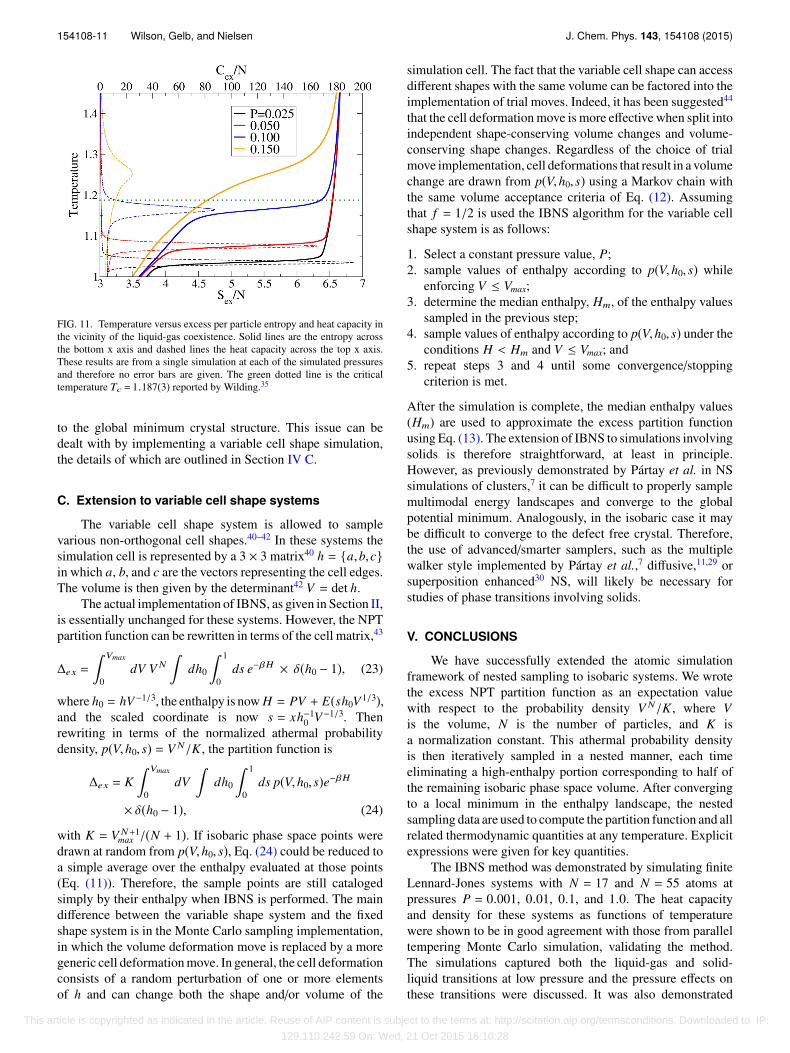
The heat capacity data were analyzed in a manner similarto that used in Section III C 4 to determine the transitiontemperatures for both the solid-liquid and liquid-gas phasetransitions. The corresponding pressure-temperature phasediagram is shown in Figure 10. The critical temperatureTc = 1.1876(3) and pressure Pc = 0.1093(6) were previouslyreported by Wilding35,36 for the same choice of potentialcutoff. Potoff and Panagiotopoulos37 later reported comparableresults, with Tc = 1.186(2) and Pc = 0.109(2). Althoughgreater than Pc, the highest simulated pressure P = 0.150displayed a small broad peak in the heat capacity at T ≈ 1.25.This is demonstrated in Figure 11, which shows the entropyand heat capacity results at each pressure in the region ofthe liquid-gas coexistence. There is some rounding of thetransition entropies due to the small system size; regardless,it is clear that the entropy no longer exhibits a tie linecorresponding to the heat capacity peak at P = 0.150 andT ≈ 1.25, which confirms that P = 0.150 is indeed abovethe critical point. Therefore, the liquid-gas coexistence curveseems to be consistent (at least within finite-size effects) withthe location of the expected critical point. The solid-liquidcoexistence temperatures systematically underestimate the tailcorrected values,38,39 which is to be expected, by roughly5%-10%. Additional contributions to the difference are finite-size effects and the fixed unit cell shape. The cubic cell shapeleads to a crystalline solid with defects that does not correspond

FIG. 10. Portion of the pressure-temperature phase diagram for the cubicunit cell periodic LJ system of 128 particles and pair-wise interaction cutoffrc = 2.5. Note that the error bars are horizontal in the temperature value.The dashed lines were added to help guide the eye. The critical pointcorresponds to the critical temperature Tc = 1.1876(3) and critical pressurePc = 0.1093(6) previously reported by Wilding.35,36

This article is copyrighted as indicated in the article. Reuse of AIP content is subject to the terms at: http://scitation.aip.org/termsconditions. Downloaded to IP:

129.110.242.59 On: Wed, 21 Oct 2015 16:10:28

154108-11 Wilson, Gelb, and Nielsen J. Chem. Phys. 143, 154108 (2015)

FIG. 11. Temperature versus excess per particle entropy and heat capacity inthe vicinity of the liquid-gas coexistence. Solid lines are the entropy acrossthe bottom x axis and dashed lines the heat capacity across the top x axis.These results are from a single simulation at each of the simulated pressuresand therefore no error bars are given. The green dotted line is the criticaltemperature Tc = 1.187(3) reported by Wilding.35

to the global minimum crystal structure. This issue can bedealt with by implementing a variable cell shape simulation,the details of which are outlined in Section IV C.

C. Extension to variable cell shape systems

The variable cell shape system is allowed to samplevarious non-orthogonal cell shapes.40–42 In these systems thesimulation cell is represented by a 3 × 3 matrix40 h = {a,b,c}in which a, b, and c are the vectors representing the cell edges.The volume is then given by the determinant42 V = det h.

The actual implementation of IBNS, as given in Section II,is essentially unchanged for these systems. However, the NPTpartition function can be rewritten in terms of the cell matrix,43

∆ex =

Vmax

0dV V N

dh0

1

0ds e−βH × δ(h0 − 1), (23)

where h0 = hV−1/3, the enthalpy is now H = PV + E(sh0V 1/3),and the scaled coordinate is now s = xh−1

0 V−1/3. Thenrewriting in terms of the normalized athermal probabilitydensity, p(V,h0, s) = V N/K , the partition function is

∆ex = K Vmax

0dV

dh0

1

0ds p(V,h0, s)e−βH

× δ(h0 − 1), (24)

with K = V N+1max /(N + 1). If isobaric phase space points were

drawn at random from p(V,h0, s), Eq. (24) could be reduced toa simple average over the enthalpy evaluated at those points(Eq. (11)). Therefore, the sample points are still catalogedsimply by their enthalpy when IBNS is performed. The maindifference between the variable shape system and the fixedshape system is in the Monte Carlo sampling implementation,in which the volume deformation move is replaced by a moregeneric cell deformation move. In general, the cell deformationconsists of a random perturbation of one or more elementsof h and can change both the shape and/or volume of the

simulation cell. The fact that the variable cell shape can accessdifferent shapes with the same volume can be factored into theimplementation of trial moves. Indeed, it has been suggested44

that the cell deformation move is more effective when split intoindependent shape-conserving volume changes and volume-conserving shape changes. Regardless of the choice of trialmove implementation, cell deformations that result in a volumechange are drawn from p(V,h0, s) using a Markov chain withthe same volume acceptance criteria of Eq. (12). Assumingthat f = 1/2 is used the IBNS algorithm for the variable cellshape system is as follows:

1. Select a constant pressure value, P;2. sample values of enthalpy according to p(V,h0, s) while

enforcing V ≤ Vmax;3. determine the median enthalpy, Hm, of the enthalpy values

sampled in the previous step;4. sample values of enthalpy according to p(V,h0, s) under the

conditions H < Hm and V ≤ Vmax; and5. repeat steps 3 and 4 until some convergence/stopping

criterion is met.

After the simulation is complete, the median enthalpy values(Hm) are used to approximate the excess partition functionusing Eq. (13). The extension of IBNS to simulations involvingsolids is therefore straightforward, at least in principle.However, as previously demonstrated by Pártay et al. in NSsimulations of clusters,7 it can be difficult to properly samplemultimodal energy landscapes and converge to the globalpotential minimum. Analogously, in the isobaric case it maybe difficult to converge to the defect free crystal. Therefore,the use of advanced/smarter samplers, such as the multiplewalker style implemented by Pártay et al.,7 diffusive,11,29 orsuperposition enhanced30 NS, will likely be necessary forstudies of phase transitions involving solids.

V. CONCLUSIONS

We have successfully extended the atomic simulationframework of nested sampling to isobaric systems. We wrotethe excess NPT partition function as an expectation valuewith respect to the probability density V N/K , where Vis the volume, N is the number of particles, and K isa normalization constant. This athermal probability densityis then iteratively sampled in a nested manner, each timeeliminating a high-enthalpy portion corresponding to half ofthe remaining isobaric phase space volume. After convergingto a local minimum in the enthalpy landscape, the nestedsampling data are used to compute the partition function and allrelated thermodynamic quantities at any temperature. Explicitexpressions were given for key quantities.

The IBNS method was demonstrated by simulating finiteLennard-Jones systems with N = 17 and N = 55 atoms atpressures P = 0.001, 0.01, 0.1, and 1.0. The heat capacityand density for these systems as functions of temperaturewere shown to be in good agreement with those from paralleltempering Monte Carlo simulation, validating the method.The simulations captured both the liquid-gas and solid-liquid transitions at low pressure and the pressure effects onthese transitions were discussed. It was also demonstrated

This article is copyrighted as indicated in the article. Reuse of AIP content is subject to the terms at: http://scitation.aip.org/termsconditions. Downloaded to IP:

129.110.242.59 On: Wed, 21 Oct 2015 16:10:28

154108-12 Wilson, Gelb, and Nielsen J. Chem. Phys. 143, 154108 (2015)

that at sufficiently high pressure (P = 1.0), the liquid-gastransition disappeared and these finite LJ systems likelyattain a supercritical fluid-like state. The increase in thetransition temperatures with pressure reported in previouspublications was confirmed. Plots of the temperature versusentropy highlighted the decreased entropy change across thephase transitions with pressure, and further analysis of the heatcapacity data allowed simple phase diagrams to be constructed.Although demonstrated on finite (non-periodic) systems, thisnew IBNS method should be easily applied to any isobaricsystem, including condensed phase systems.

Additional simulations of finite Lennard-Jones systemswith N = 17 atoms were run in order to demonstrate howvarious nested sampling parameter choices affect the simula-tion quality and thermodynamics results. In practice, an uppervolume cutoff must be imposed which sets the value of K .It was shown that the choice of the upper volume cutoff hasthe largest effect on the accuracy of the quantities directlydependent on the logarithm of the partition function, but thatthe thermodynamic quantities that depend on derivatives ofthe logarithm of the partition function are much less sensitiveto its value. Therefore, the upper volume cutoff can serve asa tunable parameter between the accuracy and efficiency ofcomputing the desired quantities. It was shown that an upperpotential energy cutoff can be enforced in conjunction withthe required upper volume cutoff. In addition, it was shownthat the Markov chain length can have a direct impact on thequality of the nested enthalpy values.

The IBNS method was further demonstrated on a simpleperiodic system consisting of Lennard-Jones particles ina cubic unit cell. A portion of the pressure-temperaturephase diagram was computed. The liquid-gas coexistencewas found to be consistent with the critical point reportedin previous studies. In addition, the update of the Monte Carlosampling scheme to simulate variable cell shape systems wasoutlined.

This new athermal method readily handles phase tran-sitions with no additional optimization and is ideal forstudying first-order phase transitions of systems under constantpressure. The isobaric nested sampling method also providesa powerful, yet straightforward alternative to NPT paralleltempering Monte Carlo. A crude relative efficiency compar-ison suggested that even with the simple sampling routineimplemented in this work, isobaric nested sampling was ableto achieve a roughly 2.5 times sampling efficiency gain overNPT parallel tempering in computing the heat capacity ofthe finite LJ systems. The use of more sophisticated andefficient sampling routines could likely dramatically increasethis efficiency gain. Further work may be done in applying theIBNS method to more complicated systems and systems withflexible simulation cells.

1A. Gelman and X.-L. Meng, Stat. Sci. 13, 163 (1998).2N. Metropolis, A. W. Rosenbluth, M. N. Rosenbluth, A. H. Teller, and E.Teller, J. Chem. Phys. 21, 1087 (1953).

3Free Energy Calculations: Theory and Applications in Chemistry andBiology, Springer Series in Chemical Physics, edited by C. Chipot and A.Pohorille (Springer, Berlin, 2007).

4T. A. Pascal, D. Schärf, Y. Jung, and T. D. Kühne, J. Chem. Phys. 137, 244507(2012).

5H. Meirovitch, Curr. Opin. Struct. Biol. 17, 181 (2007).6S. Singh, M. Chopra, and J. J. de Pablo, Annu. Rev. Chem. Biomol. Eng. 3,369 (2012).

7L. B. Pártay, A. P. Bartók, and G. Csányi, J. Phys. Chem. B 114, 10502(2010).

8J. Skilling, AIP Conf. Proc. 735, 395 (2004).9J. Skilling, J. Bayesian Anal. 1, 833 (2006).

10N. S. Burkoff, C. Várnai, S. Wells, and D. Wild, Biophys. J. 102, 878(2012).

11H. Do, J. D. Hirst, and R. J. Wheatley, J. Chem. Phys. 135, 1 (2011).12H. Do, J. D. Hirst, and R. J. Wheatley, J. Phys. Chem. B 116, 4535 (2012).13H. Do and R. J. Wheatley, J. Chem. Theory Comput. 9, 165 (2013).14S. O. Nielsen, J. Chem. Phys. 139, 124104 (2013).15L. B. Pártay, A. P. Bartók, and G. Csányi, Phys. Rev. E 89, 022302 (2014).16M. E. Tuckerman, Statistical Mechanics: Theory and Molecular Simulation,

Oxford Graduate Texts (Oxford University Press, USA, 2010).17D. Frenkel and B. Smit, Understanding Molecular Simulation, Second

Edition: From Algorithms to Applications, Computational Science, 2nd ed.(Academic Press, 2001).

18E. Marinari and G. Parisi, EPL 19, 451 (1992).19M. Saito and M. Matsumoto, in Monte Carlo and Quasi-Monte Carlo

Methods 2008, edited by P. L’ Ecuyer and A. B. Owen (Springer, BerlinHeidelberg, 2009), pp. 589–602.

20D. Sabo, D. L. Freeman, and J. D. Doll, J. Chem. Phys. 122, 094716 (2005).21F. Calvo and J. P. K. Doye, Phys. Rev. B 69, 125414 (2004).22W. D. Kristensen, E. J. Jensen, and R. M. J. Cotterill, J. Chem. Phys. 60,

4161 (1974).23H.-P. Cheng, X. Li, R. L. Whetten, and R. S. Berry, Phys. Rev. A 46, 791

(1992).24W. Ortiz, A. Perlloni, and G. E. López, Chem. Phys. Lett. 298, 66 (1998).25F. H. Verhoek, J. Chem. Educ. 47, 286 (1970).26V. A. Mandelshtam and P. A. Frantsuzov, J. Chem. Phys. 124, 204511 (2006).27J. P. K. Doye, M. A. Miller, and D. J. Wales, J. Chem. Phys. 111, 8417 (1999).28A. Barducci, G. Bussi, and M. Parrinello, Phys. Rev. Lett. 100, 020603

(2008).29B. J. Brewer, L. B. Pártay, and G. Csányi, Stat. Comput. 21, 649 (2011).30S. Martiniani, J. D. Stevenson, D. J. Wales, and D. Frenkel, Phys. Rev. X 4,

031034 (2014).31N. Chopin and C. P. Robert, Biometrika 97, 741 (2010).32D. A. Kofke, J. Chem. Phys. 121, 1167 (2004).33H. G. Katzgraber, S. Trebst, D. A. Huse, and M. Troyer, J. Stat. Mech.:

Theory Exp. 2006, P03018 (2006).34R. W. Henderson and P. M. Goggans, AIP Conf. Proc. 1636, 100 (2014).35N. Wilding, Phys. Rev. E 52, 602 (1995).36N. Wilding and K. Binder, Phys. A 231, 439 (1996).37J. J. Potoff and A. Z. Pangiotopoulos, J. Chem. Phys. 109, 10914 (1998).38G. C. McNeil-Watson and N. B. Wilding, J. Chem. Phys. 124, 064504

(2006).39E. A. Mastny and J. J. de Pablo, J. Chem. Phys. 127, 104504 (2007).40M. Parrinello and A. Rahman, J. Appl. Phys. 52, 7182 (1981).41R. Najafabadi and S. Yip, Scr. Metall. 17, 1199 (1983).42S. Yashonath and C. N. R. Rao, Mol. Phys. 54, 245 (1985).43G. J. Martyna, D. J. Tobias, and M. L. Klein, J. Chem. Phys. 101, 4177

(1994).44J. de Graaf, L. Filion, M. Marechal, R. van Roij, and M. Dijkstra, J. Chem.

Phys. 137, 214101 (2012).

This article is copyrighted as indicated in the article. Reuse of AIP content is subject to the terms at: http://scitation.aip.org/termsconditions. Downloaded to IP:

129.110.242.59 On: Wed, 21 Oct 2015 16:10:28