Neighborhood Disorganization and Police Decision-Making in ...

University of South CarolinaScholar Commons

Theses and Dissertations

2014

Neighborhood Disorganization and PoliceDecision-Making in the New York City PoliceDepartmentAllison CarterUniversity of South Carolina - Columbia

Follow this and additional works at: https://scholarcommons.sc.edu/etd

Part of the Legal Studies Commons

This Open Access Dissertation is brought to you by Scholar Commons. It has been accepted for inclusion in Theses and Dissertations by an authorizedadministrator of Scholar Commons. For more information, please contact [email protected].

Recommended CitationCarter, A.(2014). Neighborhood Disorganization and Police Decision-Making in the New York City Police Department. (Doctoraldissertation). Retrieved from https://scholarcommons.sc.edu/etd/2750

https://scholarcommons.sc.edu?utm_source=scholarcommons.sc.edu%2Fetd%2F2750&utm_medium=PDF&utm_campaign=PDFCoverPages

https://scholarcommons.sc.edu/etd?utm_source=scholarcommons.sc.edu%2Fetd%2F2750&utm_medium=PDF&utm_campaign=PDFCoverPages

https://scholarcommons.sc.edu/etd?utm_source=scholarcommons.sc.edu%2Fetd%2F2750&utm_medium=PDF&utm_campaign=PDFCoverPages

http://network.bepress.com/hgg/discipline/366?utm_source=scholarcommons.sc.edu%2Fetd%2F2750&utm_medium=PDF&utm_campaign=PDFCoverPages

https://scholarcommons.sc.edu/etd/2750?utm_source=scholarcommons.sc.edu%2Fetd%2F2750&utm_medium=PDF&utm_campaign=PDFCoverPages

mailto:[email protected]

NEIGHBORHOOD DISORGANIZATION AND POLICE DECISION-MAKING IN THE

NEW YORK CITY POLICE DEPARTMENT

by

Allison Carter

Bachelor of Arts

California State University, Fullerton, 2007

Master of Science

Arizona State University, 2010

Submitted in Partial Fulfillment of the Requirements

For the Degree of Doctor of Philosophy in

Criminology and Criminal Justice

College of Arts and Sciences

University of South Carolina

2014

Accepted by:

Robert J. Kaminski, Major Professor

Scott Wolfe, Committee Member

John D. Burrow, Committee Member

Steven Liu, Committee Member

Lacy Ford, Vice Provost and Dean of Graduate Studies

ii

© Copyright by Allison Carter, 2014

All Rights Reserved.

iii

DEDICATION

I dedicate my dissertation to my family; I could not imagine life without their

continual support. I cannot express the gratitude I have for my parents, David and Gayle,

who have both provided immense financial and emotional assistance throughout my

entire college career. Without them, this degree would not have been possible.

My father has been the backing that every young person deserves. He not only

moved me cross-country and provided the financial support to make my dreams come

true, but has had faith in me at every step of my degree. He taught me to always keep my

head up and aim high, no matter the challenges you may face. Thank you, Dad.

My mother has given me the motivation and reassurance to complete my

doctorate degree, expressing her utmost confidence in my abilities. At times, she served

as my backbone during my degree, always able to see the light in the most difficult

situations. Her words of encouragement comforted me through all stages of my degree

and I thank her for being the woman that she is. I hope one day I can provide the same

support to my children that my mother has provided me.

Lastly, I would like to dedicate my dissertation to my best friend and husband,

Michael. Not only has he given me the confidence to succeed, but he also pushed me to

do my best to accomplish goals that I did not think were possible. He was my strength

when I was weak and, without his reinforcement, this whole process would have been an

uphill battle. Thank you for being you.

iv

ACKNOWLEDGEMENTS

I would like to acknowledge and thank the members of my dissertation committee

for providing their guidance and advice throughout this project. I thank Dr. Scott Wolfe

for allowing me to “pick his brain” and taking the time to discuss the theoretical aspects

of my dissertation; I appreciate the enthusiasm and support he provided on my topic. I

thank Dr. John Burrow for providing me with recommendations on advancing the front-

end of my dissertation; it allowed me to create a more in-depth product and truly develop

the aspects behind the study’s purpose. I thank Dr. Steven Liu for being available for any

analytical questions that arose and for guiding my statistical analyses.

Lastly, I would like to thank Dr. Bob Kaminski, for serving as my Dissertation

Chair and my Graduate Director throughout my studies. Not only has he taught me in

classes, but has also provided me with several research skills that I will use in the future.

As my Dissertation Chair, Dr. Kaminski has steered my dissertation in a direction best

suited for my area of study. I thank him for being there to answer any questions I had and

for the random talks, especially when I would stop by his office just to say hi. As my

mentor, Dr. Kaminski has been a Professor I am able to lean on and look to for guidance

throughout my doctorate degree and beyond. Thank you.

v

ABSTRACT

This dissertation examines the applicability of criminological theory to police

decision-making during police-initiated encounters with suspects. Specifically, how

indicators of social disorganization can be used to predict officers’ use of coercive action

(i.e., frisk, search, use of force, and arrest) during the street stop of suspects. I also

investigate whether neighborhood disadvantage, as a moderator, impacts suspects’

likelihood of receiving greater levels of coercive action when stopped for reasons listed

in the New York City Police Departments’ Unified Form 250 (UF-250) reports.

Three theoretical arguments connecting an officer’s decision-making in a socially

disorganized area are outlined. First, an area with an increased amount of disorganization

and crime is believed to have increased levels of police coercive activities, compared to

an organized and low crime area, simply based on the amount of police activity occurring

in these areas (e.g., Terrill and Reisig, 2003). Second, as a result of the need for police to

step in as sources of social control in disorganized areas, police may increase their use of

coercive action (e.g., Clear, Rose, Waring, and Scully, 2003). And third, officers’ heavy

workload and cynicism toward residents in socially disorganized high crime areas leads

to less police coercion in disorganized and high crime areas (e.g., Klinger, 1997).

Two research questions were examined using data collected from the New York

Police Department Stop, Question, and Frisk Database, 2011 combined with

neighborhood-level census data:

vi

(1) Does neighborhood disorganization play a role in an officer’s decision to

frisk, search, use force against, or arrest a suspect?

(2) Does concentrated disadvantage strengthen or weaken the relationship

between predictors of a stop and an officer’s decision to frisk, search, use

force against, or arrest a suspect?

Three outcomes measures were created to assess whether the contemporary measures of

social disorganization (e.g., concentrated disadvantage, residential instability, and

concentrated immigration) can be used to predict officer use of coercive action: (1) as a

dichotomy of each coercive response occurring or not occurring during the stop (2) on a

continuum of coercive action and (3) using the highest level of coercive action that

occurred during the stop.

Results from multilevel analyses of stop incidents nested within neighborhoods

confirm that certain indicators of social disorganization (e.g., concentrated immigration)

affect officer use of coercive action. However, whether concentrated disadvantage

strengthens or weakens the relationship between each stop predictor (e.g., suspect fits a

relevant description) and officer coercive action (e.g., use of force), remains unknown in

the empirical literature. The dichotomous and coercive action continuum outcomes reveal

that neighborhood disadvantage weakens the relationship between the predictors of a stop

and the likelihood of coercive action, while the highest level of coercion used outcome

reveals that neighborhood disadvantage strengthens the relationship between the

predictors of a stop and the likelihood of coercive action. The contradictory findings may

indicate inaccuracy of the UF-250 reports or a conscious decision, by officers, to report

dissimilarly in disadvantaged versus affluent neighborhoods. Nonetheless, suggestions

for future research include a deeper examination into the causes behind these

conclusions.

vii

TABLE OF CONTENTS

Dedication .......................................................................................................................... iii

Acknowledgements ............................................................................................................ iv

Abstract ............................................................................................................................... v

List of Tables ..................................................................................................................... ix

List of Figures ..................................................................................................................... x

List of Abbreviations ......................................................................................................... xi

CHAPTER 1: Introduction ................................................................................................. 1

1.1 Current Gaps in Literature Examining Police Decision-Making ............................. 4

1.2 Research Questions and Plan of the Dissertation ..................................................... 7

CHAPTER 2: Police-Citizen Interactions and Police Use of Discretion ........................... 9

2.1 A Police Officer’s Role ............................................................................................ 9

2.2 Police-Citizen Interactions ..................................................................................... 10

2.3 Police Use of Discretion in PCIs ............................................................................ 24

2.4 Conceptual Frameworks Shaping Police Use of Discretion in PCIs ...................... 28

CHAPTER 3: Theoretical Frameworks of Police Use of Discretion in PCIs................... 58

3.1 Conflict Theory ...................................................................................................... 58

3.2 Empirical Evidence of Conflict Theory Impacting Police Decision-Making ........ 69

3.3 Social Disorganization Theory ............................................................................... 71

viii

3.4 Extensions to Social Disorganization Theory ........................................................ 73

3.5 Contemporary Status of Social Disorganization Measures .................................... 83

3.6 Social Disorganization Theory Applied to an Officer’s Use of Discretion ........... 86

CHAPTER 4: Data and Methods ...................................................................................... 92

4.1 Sample .................................................................................................................... 93

4.2 Analytic Strategy .................................................................................................. 111

CHAPTER 5: Results ..................................................................................................... 119

5.1 Dichotomous Outcomes ....................................................................................... 119

5.2 Coercive Action Continuum ................................................................................. 149

5.3 Highest Level of Coercive Action Used ............................................................... 154

CHAPTER 6: Discussion and Conclusion ...................................................................... 161

6.1 Discussion of Results ........................................................................................... 161

6.2 Limitations and Future Directions ........................................................................ 173

References ....................................................................................................................... 178

Appendix A – UF-250 Report......................................................................................... 203

ix

LIST OF TABLES

Table 4.1 Description of outcome measures ......................................................................99

Table 4.2 Description of independent variables ..............................................................105

Table 5.1 Stop-level effects on officer stops (no greater coercive action used)

dichotomy ........................................................................................................................119

Table 5.2 Main and moderating effects on officer stops

(no greater coercive action used) .....................................................................................122

Table 5.3 Stop-level effects on officer frisks ...................................................................127

Table 5.4 Main and moderating effects on officer frisks .................................................129

Table 5.5 Stop-level effects on officer searches ..............................................................132

Table 5.6 Main and moderating effects on officer searches ............................................135

Table 5.7 Stop-level effects on officer use of force .........................................................138

Table 5.8 Main and moderating effects on officer use of force .......................................140

Table 5.9 Stop-level effects on officer arrests .................................................................143

Table 5.10 Main and moderating effects on officer arrests .............................................146

Table 5.11 Stop-level effects on coercive action continuum ...........................................149

Table 5.12 Main and moderating effects on coercive action continuum .........................151

Table 5.13 Stop-level effects on highest level of coercion used ordinal outcome ..........155

Table 5.14 Main and moderating effects on highest level of coercion used ordinal

outcome ............................................................................................................................157

Table 6.1 Summary of all main effects – likelihood of receiving coercive action ..........163

Table 6.2 Summary of all moderating effects – likelihood of receiving coercive

action in a disadvantaged neighborhood ..........................................................................167

x

LIST OF FIGURES

Figure 1.1 Illustration of Hypothesis 1 ................................................................................8

Figure 1.2 Illustration of Hypothesis 2 ................................................................................8

Figure 4.1 Coercive action occurring during a stop .........................................................101

Figure 4.2 Coercive action continuum .............................................................................103

Figure 4.3 Highest level of coercion used in each stop ...................................................104

Figure 4.4. Reason for the stop ........................................................................................106

xi

LIST OF ABBREVIATIONS

NYPD ............................................................................. New York City Police Department

PCI ................................................................................................ Police-citizen Interaction

UF-250 ...................................................................................................... Unified Form 250

NYPD SQF ........ New York Police Department Stop, Question, and Frisk Database, 2011

GOLM ............................................................................. Generalized Ordered Logit Model

1

CHAPTER 1

INTRODUCTION

Police officers have one of the most visible positions of authority in society. An

officer’s role is to serve and protect, while ensuring safety and wellbeing among citizens.

One of the most important aspects of the criminal justice system is police officer

decision-making, or his1 use of discretion. In each stage of an encounter with a citizen, an

officer calls upon his discretion or his freedom to decide which action is best for the

situation at hand (Wilson, 1978). Wilson (1978) explains that discretion plays a major

role in an officer’s daily routine, from the moment he responds to a call for service to the

point of using deadly force against a suspect. Although the types of encounters police

have with citizens vary extensively (e.g., providing directions, attending town hall

meetings, arresting a suspect, or becoming engaged in a fire fight), the majority of police

research examining an officer’s use of discretion focuses on coercive police activities

(see e.g., Sun, Payne, and Wu, 2008).

Coercive police activities are those that emphasize an officer’s power over

citizens and include compliance methods, such as stop and frisk (Tedeschi and Felson,

1994). Stop and frisk, also known as a Terry stop, gives an officer the right to stop,

1 For simplicity, police officers and suspects/citizens are referred to in the masculine

sense throughout this paper, even though the points made may also apply to female police

officers and/or female suspects/citizens (see e.g., Clear, 2007).

2

question, and frisk any person they feel is involved in criminal activity, a common

method for detecting illegal weapons in New York City (Harris, 1994b). Regardless of

the constitutional issues first proposed against the policy (i.e., violation of Fourth

Amendment rights), stop and frisk has remained a popular policing strategy in New York

City and has become even more widespread over the years. The 1968 Supreme Court

ruling Terry v. Ohio not only ruled that stop and frisk does not violate Fourth

Amendment rights, but also upheld an officer’s right to stop a person solely based on

reasonable suspicion (Terry, 1968).

The New York City Police Department’s (NYPD) stop and frisk policy has been

one of the most controversial uses of an officer’s coercive power. The NYPD’s stop and

frisk policy was designed to control low-level disorder, however, it is often argued that

officers misuse their discretionary authority in these stops. Scholars have recognized the

potential for disparities in stops among racial minorities, arguing that minorities make up

a significant amount of police stops (e.g., Gelman, Fagan, and Kiss, 2007). Further,

scholars have also found a relationship between a neighborhood’s level of social and

economic disadvantage and an officer’s use of coercive activity (e.g., Terrill and Reisig,

2003). Due to the potential inequality in the application of stop and frisks, a common

theme among police researchers is to examine the motives that drive an officer’s

discretion during a police-citizen interaction (PCI).

Researchers argue that several factors influence an officer’s discretion during a

PCI (see National Research Council, 2004). Specifically, researchers have observed four

conceptual frameworks that influence an officer’s use of discretion: (1) the situational

dynamics of the incident, including the suspect’s race and behavior; (2) the officer’s

3

individual traits and personality; (3) the type of organization in which the officer works;

and (4) the structural features of the community (e.g., socioeconomics and demographics)

in which the officer works (National Research Council, 2004). Community characteristics

are thought to be more statistically consistent in explaining an officer’s decision to act

coercively, compared to the other conceptual frameworks (National Research Council,

2004). Although scholars have attempted to explain an officer’s decision-making using

the structural components of the community (e.g., concentrated disadvantage), the role of

macro-level criminological theory applied to police decision-making remains

understudied.

Some scholars have applied criminological theories, normally used to explain

crime, to explain an officer’s decision-making processes (e.g., Gelman et al., 2007; Kane,

2002). Conflict theory, posits that the dominant group in society creates laws to keep the

minority populations powerless (Khruakham and Hoover, 2012). Researchers examining

police decision-making from a conflict perspective argue that officers use coercive

activities in order to maintain the status of the dominant group in society (Sun et al.,

2008). Studies, however, have provided mixed results of the effects of a community’s

minority population on an officer’s use of coercion (e.g., Lee, Jang, Yun, Lim, and

Tushaus, 2010; Sun et al., 2008).

Social disorganization theory has also been used to explain an officer’s decision-

making (Kane, 2002). As a theory predicting criminal behavior, social disorganization

theory argues that the structural features of the community create an environment

conducive for criminal activity (Shaw and McKay, 1942). The amount of crime within

the disorganized community, along with the lack of informal social controls are,

4

arguably, theoretically connected to an officer’s decision-making processes. First, an area

with an increased amount of disorganization and crime is believed to have increased

levels of police coercive activities, compared to an organized and low crime area (e.g.,

Terrill and Reisig, 2003). Second, scholars have argued how the lack of informal social

controls in a disorganized neighborhood may increase the use of police coercion (e.g.,

Clear, Rose, Waring, and Scully, 2003). And third, research has also recognized the

potential for police to use less coercion in disorganized and high crime areas because of

their increased workload and cynicism toward residents (e.g., Klinger, 1997).

Over the years, scholars have created contemporary measures that can now be

used to test community disorganization (i.e., concentrated disadvantage, immigration

concentration, and residential instability) (e.g., Sampson, Raudenbush, and Earls, 1997).

Although several studies have addressed how the structural features of the community

(e.g., disadvantage) influence police decision-making (see National Research Council,

2004), to date, no study has examined the influence of social disorganization on the

relationship between predictors of a stop (e.g., suspect fits a relevant description) and an

officer’s use of coercion that may occur during a PCI (e.g., frisk, search, use of force, or

arrest). That is, how neighborhood disorganization impacts (or moderates) the

relationship between the reason for the suspect being stopped and the coercive action the

officer uses during the stop, remains unknown.

1.1 Current Gaps in Literature Examining Police Decision-Making

Scholars have long addressed the potential factors that influence an officer’s

decision-making processes (see Sherman, 1980; National Research Council, 2004). The

majority of scholars who have tested these factors, unfortunately, have found mixed

5

results (National Research Council, 2004). On the one hand, situational factors (e.g.,

suspect’s race), officer characteristics, and organizational factors alone have not proven

to significantly impact an officer’s discretion in PCIs. On the other hand, community

factors (e.g., neighborhood disadvantage) have proven to be stronger predictors of an

officer’s use of discretion. Further, researchers suggest that where an officer works

shapes his discretion in PCIs (Smith, 1986; Terrill and Reisig, 2003).

According to Terrill and Reisig (2003), the amount of literature examining how

neighborhood structural features shape police discretion is relatively scant, compared to

literature examining the other influencing factors (situational, officer characteristics, and

organizational). The authors do, however, recognize an overall theme among the

neighborhood context literature; police decision-making is driven by the features of the

environment, which “may result in suspects encountered in disadvantaged and high-crime

neighborhoods being subjected to higher levels of force. It may also result, however, in

less forceful behavior” (p. 297). For example, Terrill and Reisig’s (2003) study found that

officers were more inclined to use coercion in areas marked by high disadvantage and

high crime, while Klinger (1997) argued that areas with higher disadvantage and crime

would be subjected to less coercive police action. Other scholars have examined the

relationship between community-level features and an officer’s decision-making. In his

1986 study, Smith proposed the “neighborhood context hypothesis” and argued that

where an officer works shapes his discretion. Specifically, Smith concluded that officers

use more coercion in low-income and racially heterogeneous neighborhoods. Contrasting

Smith’s (1986) propositions, Klinger (1997) developed an ecological theory of police

behavior, stating that officers will be more lenient in these areas because crime is more

6

commonplace; Khruakham and Hoover (2012) confirmed Klinger’s ecological theory.

What is largely missing from the police literature, however, is an analysis of the

applicability of social disorganization, normally used to explain crime, to an officer’s

decision-making processes.

Kane (2002) observed that social disorganization and conflict theories could be

used to explain an officer’s behavior. In examining whether police misconduct (e.g.,

bribery) is shaped by the environment in which he works, Kane (2002) argued that the

same factors that shape a resident’s decision to act deviant (e.g., neighborhood

disadvantage) can be used to explain an officer’s malpractice. Kane’s research, however,

does not fully explain how neighborhood factors shape police decision-making in a PCI.

A study has not yet applied the three contemporary measures of social disorganization

(concentrated disadvantage, concentrated immigration, and residential instability) to

explain an officer’s coercive activity during a street encounter (e.g., frisk, search, use

force against, or arrest a suspect).

Additionally, research has not examined the possible moderating effects between

predictors of a stop and an officer’s decision-making. In 2008, Sun et al. analyzed

whether neighborhood concentrated disadvantage moderated the relationship between a

citizen’s behavior and an officer’s coercive and noncoercive responses (e.g., providing

physical assistance). They found that the relationship between a citizen’s irrational

behavior and an officer’s noncoercive action was strengthened by concentrated

disadvantage. That is, an officer was more likely to use noncoercive responses toward

irrational citizens encountered in disadvantaged neighborhoods. However, the authors did

not find significant results for concentrated disadvantage alone impacting the relationship

7

between a citizen’s demeanor and an officer’s coercive action. Sun et al. (2008), though

representing a relevant significant step forward in the analysis of social disorganization

theory predicting police behavior, still does not uncover the degree that social

disorganization strengthens (or weakens) the relationship between the stop predictors and

an officer’s decision to act coercively in a PCI.

1.2 Research Questions and Plan of the Dissertation

This dissertation aims to provide insight into whether social disorganization

theory can predict an officer’s decision-making processes. Chapter 2 opens with a brief

discussion on the role of a police officer in a contemporary society and how it sets the

stage for an officer’s responsibilities while serving his community. The chapter then

provides a literature review identifying the types of encounters the police may have

during interactions with citizens, with a focus on the most common types of coercive

police responses (e.g., stop and frisk, search, use of force, and arrest). As a typical

coercive action used by the NYPD and its potential for discrimination, the infamous stop

and frisk policy is discussed in detail. Reasons behind an officer’s decision-making

processes during a PCI are then examined and analyzed, using the conceptual

frameworks that shape an officer’s use of discretion (situational factors, officer

characteristics, organizational factors, and community characteristics). Chapter 3

explores the theoretical frameworks used in explaining an officer’s decision-making, with

a focus on how theories normally used to explain crime can be used to explain police

decision-making.

Chapter 4 discusses the proposed data collection and analytic strategy for this

research. Among other things, this research will use data collected from the NYPD Stop,

8

Question, and Frisk database, combined with data from the U.S. Census. There are two

primary research questions of interest, described below. Figures 1.1 and 1.2 represent

illustrations for each hypothesis.

(1) Does neighborhood disorganization shape an officer’s decision to frisk,

search, use force against, or arrest a suspect?


between the predictors of a stop and an officer’s decision to frisk, search, use


Neighborhood-level/

Level-2 Neighborhood disorganization

Stop-level/

Level-1 Reasons for stop Coercive action

Figure 1.1 Illustration of Hypothesis 1

Neighborhood-level/

Level-2 Concentrated disadvantage

Stop-level/

Level-1 Reasons for stop Coercive action

Figure 1.2 Illustration of Hypothesis 2

Analyses will proceed using multi-level modeling and Chapter 5 will discuss the findings

reported from the analyses. The dissertation will conclude with Chapter 6 that provides a

discussion of the importance of the current research in the broader context of policing.

9

CHAPTER 2

POLICE-CITIZEN INTERACTIONS AND POLICE USE OF DISCRETION

2.1 A Police Officer’s Role

In 1980, Black recognized that police work is a profession with its own

subculture, stratification, progress, socialization, and politics. The profession is unlike

any other in that an officer dedicates his life to serving the public and protecting people

from harm. Not only must he be a leader and enforce the laws but he must also be

someone who the public can trust to save lives and apply justice (Black, 1980).

According to Van Maanen (1978b), there are two occupational perspectives that

provide insight into a police officer’s work life. The outsider perspective focuses on the

policeman’s position in society. In his uniform, he provides a unique role to the extent

that he is constantly under public scrutiny and he may generate anxiety among the public.

At the same time, he is protecting himself and others from harm (see also Skolnick’s

1966 discussion of police solidarity and social isolation). A second perspective, the

survival method, the officer pursues a safe, yet active, routine where he also must learn

not to expect much from the job and to play by the rule of law (Van Maanen, 1978b). An

officer’s working personality is not only based on the balance between the two

occupational perspectives, but also incorporates elements of both his authoritative and

protective roles in society.

10

Skolnick (1966) summarizes the development of an officer’s working personality,

stating, “The police officer’s role contains two principle variables, danger and authority,

that should be interpreted in the light of a ‘constant’ pressure to appear efficient” (p. 43).

Danger generates the officer’s natural suspicion, while authority becomes his means to

prevent danger, allowing him to enforce the law when necessary. Muir (1977) and Reuss-

Ianni and Ianni (1983) also emphasize that an officer’s self-defensive reactions and “gut”

feelings play a role in forming his working personality.

The police officer’s role encompasses a variety of responsibilities; the National

Research Council (2004) reports that 65% of police work is comprised of responding to

citizens’ calls for service. An officer’s main goal, however, is to maintain order within

society - to control and prevent citizen behaviors that disturb the peace (e.g., public

drunkenness or loud noises). Therefore, both police researchers and the public are most

concerned with the interactions the officer has with citizens and exactly how the officer

“controls” citizens’ behaviors.

2.2 Police-Citizen Interactions

The types of encounters police have with citizens vary extensively. According to

the National Research Council (2004), an officer’s daily function includes a multitude of

actions and engagements with citizens; no two days are the same. An officer’s daily

responsibilities vary, yet the central element of police authority, managing relationships

with citizens while seeking their compliance, is an everyday occurrence (Reiss and

Bordua, 1967). When police interact with citizens, Manning (1977) describes that officer

behavior should be characterized by “proper emotional tone, proper attitude, control of

information, efficacious tactics, and skill in the manipulation and use of objects” (p. 233).

11

PCIs may be categorized into two types, based on the officer’s response to the

interaction; coercive and noncoercive police action (Sun et al., 2008).

Noncoercive police action consists of citizen support, such as physical assistance

and providing legal advice to citizens (Sun et al., 2008). Researchers have concluded that

the majority of PCIs can be categorized as noncoercive action and involve police service

situations (Black, 1980; Mastrofski, 1983; Wilson, 1978). However, because of their

potential to be harmful and/or discriminatory toward citizens, coercive police action is

the focus behind many studies involving PCIs, and is the central element of the current

paper.

An essential role of a police officer is to maintain order within society (National

Research Council, 2004). In some situations (e.g., dealing with a suspected criminal), an

officer has the right to use coercive action to control citizen conduct (Bittner, 1990).

Coercive actions may involve frisking or searching a citizen, interrogation, arrest or use

of restraints (e.g., handcuffs), and drawing/discharging a weapon (see Sun et al., 2008).

Police use coercive actions in order to establish their social identity and protect their role

in society, what Tedeschi and Felson (1994) refer to as social interactionism. Social

interactionism is a theory of coercive actions that (1) interprets coercive action as social

influences (i.e., intended to change the behavior of a person) and (2) emphasizes the

social interaction between the officer and the noncompliant citizen (Tedeschi and Felson,

1994).

Types of Coercive Police Actions

In order to serve and protect, an officer must make it a priority to gain citizen

compliance, sometimes through coercive police action (Sun et al., 2008). Common

12

coercive actions police use most often include: stop and frisk, search, an officer’s use of

force, arrest, and traffic stops (e.g., Ridgeway, 2007). Although traffic stops are one of

the most frequent coercive encounters citizens have with police (Ingram, 2007),

researchers believe they should be treated separately from street encounters (see Smith

and Visher, 1981; Klinger, 1996b).2

Stop and Frisk. In 1964 the New York State legislature adopted a new “stop and

frisk” policy that allowed police to stop and question any person in a public space, based

on the officer’s suspicion of involvement in a crime (Ronayne, 1964). Stop and question

occurs when an officer becomes suspicious of a person, stops the person (temporarily

detaining them) and questions the person about potential involvement in a crime (e.g.,

what the person is doing at the time, where the person is headed, etc.) (Spitzer, 1999).

The officer may have decided to question the person based on feelings of distrust,

initiated by the citizen’s furtive movements (e.g., walking between parked cars and

looking into their windows), the citizen’s inappropriate attire (e.g., wearing a trench coat

in the summer), the visible outline of a weapon on the citizen, or any other circumstance

that may pose a threat to the well-being of the officer or others; the official stop,

however, must be based on lawful circumstances (Spitzer, 1999). For example, an officer

may not stop a person based exclusively on his type of clothing, but may decide to stop a

2 Unless otherwise noted, the empirical literature referenced throughout this paper

includes findings from police-citizen interactions during street encounters (e.g.,

pedestrian stops) and excludes studies analyzing motor vehicle stops. Note that some

studies do not include a detailed description of data. For example, Smith and Klein

(1983) state, “police-citizen contacts were observed and recorded by trained civilians

riding on 900 patrol shifts” but do not specifically state whether these encounters include

or exclude motor vehicle stops (p. 74). Studies without a detailed data description are

assumed to be applicable to the current paper.

13

person because the person is near the scene of a recent crime and fits the description of

the suspected criminal.

Since its enactment in 1964, the stop and frisk policy has been scrutinized for its

vagueness and potential for unconstitutionality. Sindell (1966) reported, “Already those

interested in the preservation of freedom of privacy are pitted against those who clamor

for greater police protection and laws to facilitate this end. There are those who feel that

the statute dangerously impinges upon their civil liberties and is in violation of the Fourth

Amendment” (p.180). Addressing constitutional rights set forth in the Fourth

Amendment, the 1968 Supreme Court case Terry v. Ohio set the stage for the stop and

frisk policy we know today.

In 1967 a Cleveland police officer, McFadden, suspected Terry (the defendant)

and two other men of criminal activity, stopped them, frisked them, arrested them, and

charged them with carrying concealed weapons (Terry, 1968). Although Officer

McFadden’s suspicions of criminal activity were correct, the stop occurred without

probable cause, the requirement under the law in 1967. Terry, an African-American man,

claimed his constitutional rights had been violated and filed an appeal, which resulted in

the case being upheld in the state’s appeals court. Later appealed to the Supreme Court of

Ohio in 1968, the conviction of the defendant was affirmed (Terry, 1968).

Terry v. Ohio effectively reduced the volume of evidence required of police

officers to stop and frisk a citizen. Prior to the 1968 ruling, a stop and frisk required

probable cause, or the officer’s belief that the searching officer will uncover evidence of

criminal activity (Barrett, 1998). The ruling allowed officers to stop and frisk any person

they felt was reasonably suspicious of being involved in criminal activity (Terry, 1968).

14

Several lower court rulings have also addressed who may be frisked and the

circumstances that justify a frisk. Sibron v. New York was decided the same day as Terry

v. Ohio. In the case, Sibron (the defendant) was arrested and charged with possession of

narcotics. Sibron filed a motion to suppress the narcotics evidence as illegally seized. It

was ruled by the trial court that the arresting officer had probable cause to make the

arrest; the ruling was upheld by the state appellate court and later by the New York Court

of Appeals (Sibron, 1968). Sibron addressed the circumstances that substantiate a lawful

stop and frisk; the case hashed out the difference between an officer’s “reasonable

suspicion” and an officer’s “hunch.”

Since Terry v. Ohio, courts have heard several cases related to stop and frisk

policies (e.g., Adams v. Williams, Ybarra v. Illinois, Minnesota v. Dickerson). Overall,

Terry permitted certain police actions during encounters with citizens (e.g., right to stop

based on reasonable suspicion), while Sibron limited police power (e.g., stop cannot be

based on a “hunch”). Several case appeals since the 1960’s have ensured that officers act

in accordance with the law.

In its most basic form, a stop and frisk may be conducted when the officer feels

there is reasonable suspicion of criminal activity (Terry, 1968). Furthermore, as set forth

in Sibron, the officer must have reasonable suspicion that a crime has been or will be

committed, which includes “specific and articulable facts,” not solely “a hunch” (U.S.

Commission on Civil Rights, 2013, p.1). For example, the Supreme Court ruling Illinois

v. Wardlow (2000) ruled that a person fleeing at the sight of police in a high crime area is

enough to constitute reasonable suspicion. Once the stop and questioning of the person

has occurred, a frisk may (or may not) occur, depending on the officer’s suspicion that

15

the person has been, or will be, involved in criminal activity (Spitzer, 1999). The act of

frisking involves “patting down,” or moving the hands quickly over the person’s body in

order to detect weapons or other illegal contraband (Harris, 1994a).

The NYPD is well known for its aggressive policing strategies in PCIs, especially

for pedestrian stop and frisks (Fagan and Davies, 2000). Many of the NYPD aggressive

policing strategies were derived from the theoretical foundations of Wilson and Kelling’s

(1982) broken windows theory, where community physical disorder is proposed to led to

an increase in criminal behaviors (see also Spitzer, 1999); New York City police officers

often rely on stop and frisks to address low-level disorders. Specifically, the NYPD’s

1994 Police Strategy No. 5, Reclaiming the Public Spaces of New York included

aggressively targeting minor offenses in order to control more serious violations (Fagan

and Davies, 2000). The most famous pursuit of disorder or nuisance was the “squeegee”

people in New York City during the late 1990s. The NYPD focused their efforts at

eliminating “squeegee” people that disturbed and annoyed law-abiding citizens. As Parks,

Mastrofski, DeJong, and Gray (1999) states, “Under Commissioner William Bratton,

New York City discontinued the ‘Officer Friendly’ community policing approach of the

previous commissioner in favor of a focus on rigorous law enforcement to rid the streets

of ‘squeegee men’” (p. 487). Aggressive policing on the squeegee people, however,

opened the door for an influx of aggressive policing on many types of public social

disorders (e.g., public intoxication, graffiti, and public urination) (Fagan and Davies,

2000).

Another NYPD directive, Police Strategy No. 1, Getting Guns Off the Streets of

New York focused on seizing illegal firearms in order to reduce gun violence (Fagan and

16

Davies, 2000). These two initiatives (No. 5 and No. 1) gave police ultimate power over

citizens, allowing police to stop and frisk any person they felt was suspicious or

disorderly, while still acting under the laws outlined by Terry v. Ohio. Although this led

to multiple arrests for misdemeanor offenses, it also exposed the NYPD to attacks of

discrimination. Trone (2010) reported that stop and frisk encounters within the NYPD

caused considerable debate as to whether the stops were racially biased and whether the

policy worked at reducing crime (see also Harris, 1994a, 1994b).

In situations involving stop and frisk, or more serious coercive police actions

(e.g., search, arrest, or use of force), the responding officer must fill out a Unified Form

(UF-250) report (Fagan and Davies, 2000). Depending on the circumstances of the

incident, the officer may or may not complete the UF-250 report. The NYPD Patrol

Guide mandates officers to fill out the report under four specific circumstances (1) person

is stopped by use of force (2) person stopped is frisked or frisked and searched (3) person

is arrested or (4) person stopped refused to identify himself (Spitzer, 1999). Although

non-mandated UF-250 reports make up some of the total reports, it is estimated that

mandated UF-250 reports account for approximately 72% of the total reports (Gelman et

al., 2007). The UF-250 reports provide details of each stop, on behalf of the police officer

involved; the information collected includes, but is not limited to: the officer's reasons for

initiating the stop, whether the stop led to an arrest, demographic information for the

person stopped, and the suspected criminal involvement. Appendix A provides an image

of the front and back of the NYPD’s UF-250 report.

One of the first notable studies of NYPD stop and frisk UF-250 reports in 1998

described that the number of reports more than doubled over a span of ten years (Fagan

17

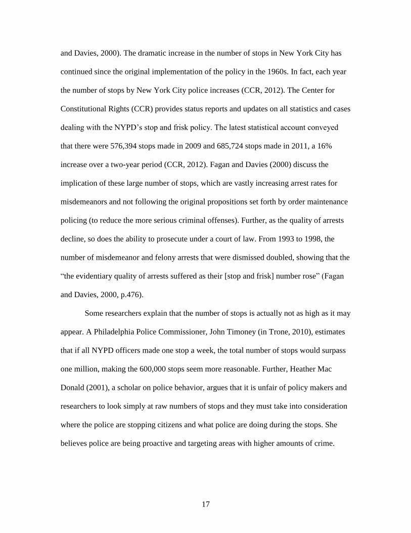
and Davies, 2000). The dramatic increase in the number of stops in New York City has

continued since the original implementation of the policy in the 1960s. In fact, each year

the number of stops by New York City police increases (CCR, 2012). The Center for

Constitutional Rights (CCR) provides status reports and updates on all statistics and cases

dealing with the NYPD’s stop and frisk policy. The latest statistical account conveyed

that there were 576,394 stops made in 2009 and 685,724 stops made in 2011, a 16%

increase over a two-year period (CCR, 2012). Fagan and Davies (2000) discuss the

implication of these large number of stops, which are vastly increasing arrest rates for

misdemeanors and not following the original propositions set forth by order maintenance

policing (to reduce the more serious criminal offenses). Further, as the quality of arrests

decline, so does the ability to prosecute under a court of law. From 1993 to 1998, the

number of misdemeanor and felony arrests that were dismissed doubled, showing that the

“the evidentiary quality of arrests suffered as their [stop and frisk] number rose” (Fagan

and Davies, 2000, p.476).

Some researchers explain that the number of stops is actually not as high as it may

appear. A Philadelphia Police Commissioner, John Timoney (in Trone, 2010), estimates

that if all NYPD officers made one stop a week, the total number of stops would surpass

one million, making the 600,000 stops seem more reasonable. Further, Heather Mac

Donald (2001), a scholar on police behavior, argues that it is unfair of policy makers and

researchers to look simply at raw numbers of stops and they must take into consideration

where the police are stopping citizens and what police are doing during the stops. She

believes police are being proactive and targeting areas with higher amounts of crime.

18

Advocates of the stop and frisk policy (e.g., some citizens, police officers,

politicians, etc.) believe that police have the right to stop and frisk whomever they feel is

suspicious and argue that the policy has positively impacted crime in New York City.

The majority of citizens, however, are skeptical of these findings, arguing that statistics

reveal that crime rates have been on the decline even before the implementation of the

strict stop and frisk policy (see Rose, 2013). For example, Fagan and Davies (2000) point

to cyclical changes in rates of violent crime and neighborhood collective efficacy as

sources of changes in crime rates. The majority of citizens also believe that the policy

violates right to privacy and is unconstitutional.

In a recent federal class action lawsuit, Floyd, et al. v. City of New York, et al.,

defendants claimed violations of the Fourth Amendment and Fourteenth Amendment

protections against unreasonable searches and seizures, racial profiling, and

unconstitutional stop and frisks (CCR, 2013a; House, 2013; Rose, 2013). On March 27,

2013, the NYPD included a memo as evidence in the case that instructed officers give a

narrative description of every stop, in addition to checking the boxes on the UF-250 form

(CCR, 2013b).

On August 12, 2013 U.S. District Judge Shira Scheindlin ruled that the NYPD’s

stop and frisk policy violated constitutional rights of citizens (CCR, 2013c). Scheindlin

(2013) stated, “the public interest in liberty and dignity under the Fourth Amendment,

and the public interest in equality under the Fourteenth Amendment, trumps whatever

modicum of added safety might theoretically be gained by the NYPD making

unconstitutional stops and frisks” (p. 5). As a result, the Judge ordered a reform to the

policy, which included the appointment of an independent monitor. The monitor is to

19

oversee the agreed-upon reforms of the policy (e.g., changes to stop and frisk

documentation) in the department, including aspects of officer training, supervision, and

discipline (CCR, 2013c).

However, these judge-ordered reforms came to a halt when New York City filed

appeals. Upon appeals, Judge Scheindlin was subsequently removed from the case, the

city arguing that the judge did not act in a fair and impartial manner (CCR, 2013c). In

November 2013, New York City adopted a new mayor, de Blasio, as well as a new Police

Commissioner, Bratton. In January 2014, de Blasio dropped the appeals and reached an

agreement with the Floyd plaintiffs (CCR, 2014). Although Bratton feels strongly that

stop, question, and frisk is a basic tool used in the NYPD, the reform process of the

policy has begun. Compared to months in the second-half of 2012, stops in the same

months in 2013 saw an 80% reduction of police stop and frisks (Long, 2013).

Search. Four years after the rulings of Terry and Sibron, a case under the Terry

ruling appeared in Connecticut. In 1972, Adams v. Williams was heard by the Court of

Appeals. Officer Adams was approached by an informant saying that the defendant,

Williams, was in possession of narcotics and an illegal firearm. When Officer Adams

approached Williams in his parked car, Williams refused Officer Adams’s requests to get

out of the car. Upon refusal, Officer Adams reached into the car and took possession of a

firearm in Williams’s waistband. Subsequent searches also revealed heroin and a machete

located in Williams’s car. Williams was convicted of possession of a handgun and

narcotics. He appealed the ruling on behalf of unlawful search. The Court of Appeals

upheld the decision that the right to stop and frisk can be based on information from other

people, not solely on behalf of reasonable suspicion by the officer (Adams, 1972).

20

Police officers have the right to search a person they believe he has been

involved, or will be involved, in a crime in order to uncover evidence or contraband

(Spitzer, 1999). A search occurs when the officer investigates, or combs through, the

suspect’s possessions or on his person (e.g., his bag or his pant pockets) (Harris, 1994a).

The Fourth Amendment protects Americans from illegal searches and seizures by police,

stating that a search must be based on probable cause, or if a search warrant has been

issued by a judge declaring probable cause for the search (U.S. Const., amend. IV). The

Supreme Court’s ruling Terry v. Ohio, however, allowed a search and seizure without

probable cause, but under circumstances of reasonable suspicion.

When discussing the difference between frisks and searches, Harris (1994a)

states, “Frisks could not go beyond a pat down of outer clothing to locate a weapon; once

the officer knew no weapon was present, further searching was improper” (p. 662). A

street encounter often begins with an officer’s stop and frisk of a suspect before

furthering into a search, however, a search does not have to originate from a frisk (Harris,

1994a). A person that is frisked will not always be searched (e.g., when there is no

reasonable suspicion that evidence will be obtained) and a person searched does not first

have to be frisked.

Use of force. Bittner (1990) recognizes that the primary activity that sets the

police apart from other government agencies is their authority to use force. Force can be

defined as the exertion of power to coerce or contain the behaviors of others (Kania and

Mackey, 1977). Brown (1981) argues that police are constantly under the unpredictable

pressures of violence from citizens stating, “the thought that violence (or the threat of it)

21

often begets violence” (p.77). A police officer, therefore, must always expect violent

behaviors and be prepared to use force to protect himself and others from harm.

Some common forms of police use of force include, but are not limited to: strong

verbal cues3, intimidation, compliance methods, physical force, and deadly force

(Klinger, 1995). Researchers have different methods for measuring police use of force

(dichotomous, ordinal, and continuous measures). The most common method is to place

the use of force actions on a continuum based on the level of force used in the encounter,

ranging from the least severe to most severe option (see e.g., Klinger, 1995; Paoline and

Terrill, 2007; Terrill and Mastrofski, 2002). It is also common practice to examine the

highest level of force used during an encounter, which allows researchers to gain an

understanding of the type of force police use to gain citizen compliance. To illustrate,

Paoline and Terrill’s (2007) study used the highest level of force that occurred in each

encounter placed on a continuum, beginning with verbal commands and threats and

ending with impact methods, such as hitting, use of baton, or stun gun (because of their

interest in citizen compliance, Paoline and Terrill excluded police use of firearms in their

study).

Police use of force has long been a central topic of research involving police

activity. Two theoretical perspectives are often used to explain an officer’s use of force

(1) sociological and (2) psychological (Terrill and Mastrofski, 2002). The sociological

perspective explains police use of force in terms of the citizen – who the citizen is and

what the citizen does – while the psychological perspective explains police use of force in

3 Following the practices of Terrill and Mastrofski (2002), this discussion includes verbal

commands as a type of force (see also Sun and Payne, 2004; Paoline and Terrill, 2005).

22

terms of the officer’s background, personal characteristics, and experiences (Terrill and

Mastrofski, 2002).4 Research on police use of force has pursued a number of avenues,

including excessive use of force (e.g., Adams, 1996; Klinger, 1995; Lee et al., 2010) and

deadly force.

A frequently studied type of police use of force is deadly force, which occurs

when a suspect is killed because of the officer’s use of force (e.g., gunshot) (Geller and

Scott, 1992). Police use of deadly force has gone through substantive changes over the

years. In order to reduce racial disparities seen in the use of deadly force in the 1960s and

1970s, police departments adopted the “defense of life” rule in the 1970s, where police

shootings became limited to situations that pose a threat to life (Garner, 1985; Walker,

Spohn, and DeLone, 2000). The defense of life rule, as estimated by Fyfe (1978), reduced

New York City police officer firearm discharges by almost 30% within a few years.

Furthermore, the 1985 Supreme Court case Tennessee v. Garner ruled the “fleeing felon

rule” unconstitutional, which accelerated the “defense of life” standard in situations

involving police use of force.

In 1985 the Supreme Court ruled on a case regarding an officer’s use of deadly

force, Tennessee v. Garner. A Memphis police officer attempted to arrest a young man,

Garner, for suspected burglary; the suspect fled the scene and was shot and killed by the

officer (Garner, 1985). Garner’s father (defendant) brought an action in Federal District

Court, arguing violation of his son’s constitutional rights. The District Court ruled that

the officer’s actions did not violate Garner’s constitutional rights; the Court of Appeals

4 For further discussion on factors affecting police coercion, refer to chapter 2.4 of this

dissertation.

23

reversed the lower court’s decision (Garner, 1985). The Court of Appeals ruled, “such

force may not be used unless necessary to prevent the escape and the officer has probable

cause to believe that the suspect poses a significant threat of death or serious physical

injury to the officer or others” (Garner, 1985, p. 7). Although not the topic of the current

paper, many researchers have addressed an officer’s use of deadly force in PCIs (see e.g.,

Klinger, 1995), especially in terms of racial disparities (Fyfe, 1982; Geller and Karales,

1981; Jacobs and O’Brien, 1998). Many of the racial disparities found, however, often

dissipate when researchers control for at-risk status (e.g., felony suspect) (Geller and

Karales, 1981).

Even though there are no specific criteria that state what a police officer must do

in each situation when it comes to use of force, Bittner (1990) explains three specific

restrictions placed on police officers. First, police use of deadly force is limited (e.g., in

life-threatening circumstances). Second, police may only use force in performance of

their duties. And third, police may not use force maliciously or frivolously (Bittner,

1990). Researchers acknowledge that officers infrequently use physical force in police-

citizen encounters and, when they do use force, they more often choose the less physical

options (e.g., Klinger, 1995 reported that voice commands were used in 58% of

“forceful” cases).

Arrest. Another common tool an officer may use during a PCI is arrest. Terrill

and Reisig (2003) define arrest as a physical restraint, where the suspect is handcuffed for

the safety of himself and/or others. An official arrest includes taking the suspect to the

police department, completing a booking sheet, a property voucher, and other paperwork

for processing; an officer’s decision to arrest must be based on probable cause (Spitzer,

24

1999). For example, an officer who searches a person and finds a handgun has the right to

arrest the person based on illegal carrying of a concealed weapon (Barrett, 1998).

An officer’s decision to arrest is one of many possible alternative coercive

actions; he has the authority to arrest and the freedom to not arrest. Black (1980) reports

that officers tend to be more lenient and use their power to arrest less frequently than the

law would permit. For example, Sun and Payne (2004) reported that only 5% of their PCI

sample resulted in arrest, with the other coercive actions (e.g., threats and restraints)

having a higher likelihood. A suspect has the highest chance of being arrested (95%) if an

officer observes the crime; all other factors (e.g., testimonial evidence and disrespectful

suspects) run a 70% chance or less of the suspect being arrested (Mastrofski, Worden,

and Snipes, 1995). In every PCI, the officer makes a choice as to which coercive action,

if any, will be used to gain citizen compliance.

2.3 Police Use of Discretion in PCIs

Throughout the training process, police officers are taught to identify suspicious

persons or behaviors and to recognize those situations that may pose a threat to their

well-being (Skolnick, 1994). These identifications and recognitions may stem from what

is called the symbolic assailant. The symbolic assailant theory was developed to explain

how officers categorize people and differentiate between citizens and suspects, based on

what most often relates to criminal activity (e.g., being an African-American young male)

(Skolnick, 1994). On top of the officer’s distinction between law-abiders and law-

breakers, the decision an officer decides to make in a situation is often based on what the

officer “feels” is appropriate (Brown, 1981). In every PCI, police have the discretion to

respond in a manner they deem fit.

25

An officer’s use of discretion can be distinguished by two characteristics (1) their

aggressiveness, or taking initiative in crime fighting and (2) their selectivity, or the

increased likelihood to enforce the law (Brown, 1981). According to Brown (1981), these

two characteristics come together to form one of four officer operational styles: selective

and highly aggressive; selective and less aggressive; non-selective and highly aggressive;

and non-selective and less aggressive (p. 224). The officer’s predisposition toward

aggressiveness and selectivity can help clarify the varying degrees (e.g., decision to arrest

versus not arrest) of an officer’s use of discretion in each PCI. That is, an officer who is

selective and highly aggressive is more likely to seek out suspects and make more arrests,

compared to an officer who is non-selective and less aggressive.

Often times, officer decision-making is not only based on the officer’s working

personality (see Brown, 1981) but also on the “type” of person present during the

interaction (Van Maanen, 1978). As stated by Van Maanen (1978), “the asshole is a part

of every policeman’s world” (p. 221). Of course Van Maanen is not referring to every

citizen in PCIs, but is referencing those who are treated harshly simply because of their

behavior during the interaction (e.g., the citizen attempts to fight or flee). Mastrofski,

Snipes, and Supina (1996) showed that people who were irrational toward police were

more likely to be noncompliant with police efforts. “The asshole,” compared to the other

typologies (“suspicious persons” and “know-nothings”) is a higher candidate for street

justice, or the officer’s use of authority aimed at correcting ill behaviors (Van Maanen,

1978).

In the decision-making process, an officer’s use of discretion takes one of two

roles - delegated or unauthorized (Skolnick, 1994). Delegated discretion is that response

26

which is clearly allowed by the police (e.g., arresting a murder suspect), while

unauthorized discretion deals with police actions where they may not have authority (e.g.,

misuse of force) (Skolnick, 1994). Problems arise when the lines of authority in delegated

discretion are unclear; not every person would agree on the correct course of action taken

by police officers, which invites scrutiny into an officer’s use of discretion (Brooks,

2001; Skolnick, 1994).

Bittner (1990) explained that a police officer’s use of discretion is based on

keeping the peace and is not founded upon direct compliance with the law. Even with the

Fourth Amendment protections against unreasonable searches and seizures, Maclin

(1998) believes that Terry v. Ohio gave officers an extraordinary amount of discretion. If

police have reason to believe the law has been broken they will have authority to stop the

person.

Skolnick (1994) recognized that specific laws are purposefully made subjective

(e.g., disturbing the peace) in order for the police officer to maintain order. Officers use

legal recourse as a tool to control unwanted behaviors by citizens, ensuring that their

discretion is in line with the appropriateness of the situation (Black, 1980). For example,

officers use less discretion in serious felony offenses and more discretion in

misdemeanors (Black and Reiss, 1970). They are also less likely to use legal recourse in

situations in which the victim and offender have a relationship (e.g., a family member),

whereas incidents involving no victim-offender relationship are more likely to be

formally handled by police (Black, 1980). An officer’s discretion encompasses the ability

to decide which rule(s) to impose on a citizen and the power to decide whether or not to

apply the rule(s); not doing something may hold as much importance as doing something

27

(Brooks, 2001). Brown (1981) recognized that an officer uses discretion as a way to

implement laws, but also acknowledged that officers are limited in their decision-making

because of laws.

From the manner with which they choose to interact with citizens to the decision

to invoke the law, police use of discretion is a subject under constant attention by

researchers (Novak, Frank, Smith, and Engel, 2002). Wilson (1978) explained that an

officer’s discretion is based on the perceived costs and benefits from the situation at hand

– “the net gain and loss to the suspect, the neighborhood, and the officer himself of

various courses of action” (p. 84). An officer’s decision-making is based on the “recipe of

rules” he has developed through his experiences as an officer. The recipe of rules acts as

a guide on how to do the job and what is acceptable to the department, but may not

always align with legal or legitimate rules (Manning, 1977).

Because police behavior is shaped my many factors (e.g., recipe of rules,

departmental policies, personal values, and social relationships), understanding police use

of discretion is a difficult undertaking. While emphasizing that discretion is based on

laws and the officer’s individual morals and beliefs, Brown (1981) stated, “In the act of

discretion, although the decision maker accepts a framework of values and goal, some

aspects of the decision process are unspecified or contingent on circumstances and thus

up to the judgment of the individual” (p. 25). Brown (1981) explained that a police

officer’s use of discretion in a PCI is under political control and constant examination as

to whether or not the officer acted “accordingly” in each situation. Police are trained to

respond to each situation in a manner they deem necessary, which is shaped by many

28

components, including the factors of the situation, the characteristics of the suspect, the

officer’s prior experiences, his department’s values, and the location of the encounter.

2.4 Conceptual Frameworks Shaping Police Use of Discretion in PCIs

An officer’s use of discretion during a PCI is driven by a variety of factors. First

and foremost, an officer’s use of discretion is heavily dependent upon the legal factors of

the situation, including evidence against the suspect, seriousness of the offense, and the

presence of a complaint (Sherman, 1980). Police are much more likely to arrest a suspect

in situations where police witness the commission of a crime, because the evidence

against the suspect is greater (Black, 1971). The seriousness of the offense also shapes an

officer’s discretion during a PCI. Mastrofski et al. (1995) reported that, compared to

minor offenses “the odds of arrest are almost ten fold when the offense is serious” (p.

551).

In some circumstances, however, police decide not to invoke formal action (e.g.,

taking a juvenile home to be punished by his parents, instead taking him to the police

station) (Ericson, 1982; Goldstein, 1960). It is when officers decide to stray from the law

and not invoke formal action that peeked police researchers’ interests. Because officers

have the freedom to decide what is “necessary” in every PCI, police discretionary

research has become very popular over the years. Researchers have investigated other

factors that drive police use of discretion, instead of focusing solely on the legal factors

that impact an officer’s decision-making.

In 1980, Sherman offered one of the first substantive evaluations of police

behavior. In his paper, he uses a framework of five approaches to explain police use of

discretion, one being legal, and the other four being extralegal. The extralegal factors

29

include: situational factors, officer characteristics, organizational factors, and community

characteristics. Following Sherman’s research, Riksheim and Chermak (1993) and the

National Research Council (2004) have also provided a summary of the extralegal factors

that shape police use of discretion. Riksheim and Chermak (1993) state that over the

years, “our understanding of the causes of police behavior has become more refined” (p.

353).

The substantive points taken from these important reviews of police discretionary

literature is that (1) situational factors, officer characteristics, organizational factors, and

community characteristics continue to be recognized as driving forces in police use of

discretion and (2) the impact of each extralegal factor on police decision-making (i.e. his

decision to act more or less coercively) is relatively unknown, with various studies

providing mixed results. The current paper, although not an exhaustive review of the

literature, examines the four factors that have been commonly attributed to shaping an

officer’s decision-making processes during a PCI.

Situational Factors

When it comes to police use of discretion, scholars have recognized that police

may act differently in each PCI. The first extralegal factor that is recognized to shape

police use of discretion is situational factors. Situational factors are the characteristics of

the situation that are unique to each PCI; these variables may include the suspect’s

gender, age, race, social class, and demeanor toward police (see Sun et al., 2008). In their

overview of PCI literature, Walker et al. (2000) state, “officer behavior is heavily

determined by the contextual or situational variables: location (high-crime versus low-

30

crime precinct); the perceived criminal involvement of the citizen; the demeanor of the

citizen; and in the case of physical force, the social status of the citizen” (p. 99).

Police often use situational characteristics to form judgments of citizens in each

PCI; these judgments construct an officer’s decision-making processes (see Berk and

Loseke, 1981). Although there have been general statements made regarding the effects

of situational characteristics shaping an officer’s use of discretion (e.g., National

Research Council, 2004; Sun et al., 2008), each situational factor (e.g., suspect gender,

race, demeanor) has been examined separately by researchers. When situational factors

are examined separately, evidence of each component shaping police use of discretion

becomes less clear. For example, in terms of the suspect’s race, the National Research

Council (2004) reported that some scholars found that, compared to whites, racial

minorities received lower amounts of police coercive action; some reported null effects;

and others reported that racial minorities received higher amounts of police coercive

action. Overall, situational factors remain an important driving force in police decision-

making processes, but the individual components that make up the situational factors

have produced mixed statistical conclusions.

Gender. The evidence regarding a suspect’s gender and an officer’s decision-

making has been inconclusive. Some scholars have reported that males are more likely to

be subjected to coercive police actions, while others reported that females are handled

more formally by police. Still others have found no significant difference between the

sexes.

Terrill and Reisig (2003), for example, controlled for several encounter-level

variables (e.g., suspect characteristics, officer characteristics, and citizen audience) and

31

found that males are more likely to be on the receiving end of police officer force. Also,

Sealock and Simpson (1998) reported that male contacts with police are more likely to

result in arrest (61.3%), compared to female contacts (37.1%). In their study, the

researchers controlled for legal factors (e.g., offense seriousness, prior police contacts,

and whether or not an officer observed the offense). Sealock and Simpson (1998) also

examined the significance of offense seriousness in arrest decisions between males and

females and concluded that offense seriousness plays a more significant role in female

arrests than it does in male arrests (15.53% versus 11.82%), showing that both legal and

extralegal factors are at play in shaping an officer’s decision-making.

Contrary to these findings, Hindelang (1979) reported that females were actually

overrepresented in arrest statistics for robbery and aggravated assault, compared to males.

According to Visher’s (1983) research, females who exhibit “appropriate gender

behaviors and characteristics” are less likely to be arrested, while women who “deviate

from stereotypic gender expectations” can be expected to be arrested more frequently (p.

5) (see also Gelsthorpe, 1986).

In the meanwhile, Smith and Visher (1981) examined PCIs from 24 metropolitan

police departments and concluded, in terms of arrest and controlling for other factors

(e.g., suspect demeanor), “police do not discriminate in favor of women” (p. 174); their

research reported that males and females had an equal chance of being arrested. The main

point taken from these reports on how a suspect’s gender impacts an officer’s use of

discretion is that an officer’s coercive action may or may not be driven by gender;

empirical evidence on the subject remains mixed.

32

Age. Police researchers have also examined the impact of the suspect’s age on

police coercive action. Brown, Novak, and Frank (2009) examined the impact of age on

an officer’s decision to arrest. Controlling for the suspect’s race, gender, intoxication,

demeanor, offense type, and whether the officer witnessed the crime, they found that

juveniles (under the age of 18) ran a higher risk of being arrested than adults. These

findings, however, did not hold when the location of the encounter was factored in;

juveniles encountered in distressed communities were more likely to be arrested, while

adults encountered in less distressed communities were more likely to be arrested.

In partial support of Brown et al.’s findings, Terrill and Reisig (2003) found a

positive relationship between younger suspects and police coercion (measured as a

continuum of force). However, contrary to Brown et al., Terrill and Reisig reported that

police use of force was more often applied to younger suspects, regardless of

neighborhood context. Likewise, Terrill and Mastrofski’s (2002)5 study of situational

determinants on police use of force (verbal and physical forms) revealed that younger

suspects (age measured on an ordinal scale) are more likely to be subjected to higher

levels of force, controlling for the suspect’s other characteristics (e.g., demeanor), the

number of officers and bystanders present during the PCI, the anticipation of violence

(through the dispatcher’s indication), and whether the PCI occurred in a community-

oriented or traditional policing style jurisdiction.

5 Terrill and Mastrofski’s (2002) study analyzed data from the Project on Policing

Neighborhoods (POPN) that incorporated both street and motor vehicle police-citizen

encounters, but it is unclear which type of encounter dominates the analyses.

33

On the other hand, studies also report a negative, or even insignificant,

relationship between the suspect’s age and police coercive behaviors. For example,

Lundman (1974) found no statistically significant differences between juvenile and adult

arrest rates, controlling for citizen race, social class, and the location of the encounter.

Similarly, Sun and Payne (2004) reported that youthful suspects (age 18-29 years old) did

not impact the officer’s decision to use coercive action (measured on a continuum of use

of force). Moreover, in their study of NYPD arrest decisions, Khruakham and Hoover

(2012) found that older suspects were more likely to be arrested than youth, net of other

situational-level variables. Similar to literature examining the impact of suspect gender

on police decision-making, the impact of the suspect’s age on police use of discretion

remains inconclusive.

Social Class. Bittner (1990) argued that an officer is not concerned with the

connections between economic inequality and criminality and that an officer does not

purposefully seek to enforce the laws differently for certain types of people. However,

research in this area, more often than not, supports the notion that suspects of low-income

status can expect to receive more severe and more punitive police responses (Black,

1976, 1980). Several scholars have provided empirical support for the finding that people

in lower socio-economic statuses receive harsher treatment by police.

Terrill and Mastrofski’s (2002) study of situational determinants on police use of

force (verbal and physical forms) showed that higher levels of force are more often

applied to economically poor suspects, net of other factors (e.g., suspect demeanor,

anticipation of violence, jurisdiction). Terrill and Reisig (2003) also reported a positive

relationship between lower class individuals and rates of arrest, irrespective of other

34

situational characteristics and neighborhood context. Further, Sun et al.’s (2008)

multilevel analysis of factors impacting police behavior revealed that, compared to

affluent citizens, poor citizens were more likely to be subjected to police coercive

activities (e.g., searching the suspect, police discharging a weapon).

Overall, most research supports the notion that a suspect’s social class will factor

into an officer’s use of discretion, although some studies contradict the consensus that

suspects in a lower social class receive more coercive police action. For example,

Mastrofski et al. (1995) uncovered that police treated the poor less harshly. The authors

conveyed their perplexity by stating that officers are “less likely to arrest when the

suspect is poor is a puzzle” (p. 555). This seems to reveal that some other extralegal

factors are at play; possibly other factors (e.g., community characteristics) have a more

influencing impact on shaping an officer’s use of discretion.

Race. The majority of empirical evidence examining police use of discretion

indicates that minorities receive harsher treatment by police. For example, Smith and

Visher (1981) reported that African-Americans are more likely to be arrested, net of other

factors (including offense seriousness and suspect demeanor). Also, Sealock and

Simpson’s (1998) study reported racial bias in arrest practices and stated that African-

Americans were more likely to be arrested than whites, while taking other factors into

consideration (e.g., offense seriousness). Later, Terrill and Mastrofski’s (2002) study of

situational determinants on police use of force (verbal and physical forms) showed that

racial minorities have a higher chance of being on the receiving end of increased force,

controlling for several other predictors (e.g., suspect’s demeanor, number of bystanders,

and jurisdiction).

35

Some studies, however, do not follow this pattern. Geller and Karales (1981)

examined racial disparities in police shootings and found that when they controlled for at-

risk status (defined as forcible felony arrest), whites were subjected to deadly force more

often than minorities. Further, Mastrofski, Reisig, and McCluskey (2002) examined

police officer disrespect towards whites and minority citizens and showed that whites

received harsher treatment by police. In their study, police officer disrespect was

measured as illegitimate speech and gestures that target the citizen’s identity; the authors

revealed that in St. Petersburg, whites received more police disrespect than minorities,

controlling for neighborhood context. Although police officer disrespect is not considered

a specific type of coercive action, per se, it is argued that these findings are applicable to

the current review. Mastrofski et al. (2002) noted that some research observers code more

serious forms of police misbehavior (e.g., excessive force) as police disrespect. Further,

the authors’ hypotheses are guided by findings from prior literature examining the effects

of situational factors on an officer’s use of coercive action (e.g., arrest).6

In terms of the suspect’s race impacting an officer’s use of discretion, some

studies have provided null findings. In their study of community policing, Mastrofski,

Worden, and Snipes (1995) reported that race had no statistically significant impact on an

officer’s decision to arrest a suspect. Also, Garner, Maxwell, and Heraux (2002)

examined the influence of situational factors on police use of force (verbal commands to

6 In forming their hypotheses, Mastrofski et al. (2002) discussed findings from studies

reporting on situational factors impacting police use of coercion in order to estimate

influences on police disrespect. For example, they hypothesized that police would exhibit

higher amounts of disrespect toward minority citizens and they cited Black’s (1976)

predictions that certain groups of society would be subjected to an increase in punitive

action by the criminal justice system.

36

use of a weapon) from six law enforcement agencies. They reported that the difference in

use of force between whites and nonwhites was statistically insignificant, even after

controlling for the suspect’s resistance. Again, it may be that research on the suspect’s

race shaping an officer’s decision-making is mixed because other extralegal factors that

are not the focus of these particular studies (e.g., community characteristics) potentially

have a greater impact in shaping an officer’s decision-making processes.

Suspect Demeanor. Unlike demographic characteristics, citizen demeanor has

proven to be a stronger and more consistent situational predictor of police decision-

making during a PCI (e.g., Mastrofski et al. 2002). The majority of research examining

situational factors impacting police coercive action concludes that citizens who exhibited

disrespectful or irrational behavior toward police were subjected to an increase in police

coercive actions (e.g., Reiss, 1968; Sun et al., 2008). Disrespectful or irrational behavior

on behalf of the citizen includes discourteous actions directed at police, such as ignoring

police commands, displaying obscene gestures, and making derogatory remarks (see e.g.,

Sun and Payne, 2004).

Reiss (1968) was one of the first scholars to examine data from an observational

study of police use of nonlethal force in Chicago, Boston, and Washington, D.C. He

concluded that a suspect who acted defiantly had a higher likelihood to be on the

receiving end of nonlethal force. Following Reiss’s (1968) study, Friedrich (1977)

reanalyzed the observational data in a more comprehensive manner (i.e., he examined the

relationship between organizational, situational, and individual factors and police

behavior). Friedrich (1977) reported that one out of every three suspects arrested

37

displayed antagonistic behavior toward police, while those whose behavior was civil ran

a one out of seven risk of arrest.

The surge of research examining the impact of suspect demeanor on an officer’s

decision-making also brought skepticism to the validity of findings. In his 1994 article,

Klinger criticized prior studies’ measurements of suspect demeanor because of their

inclusion of both noncriminal and criminal behaviors. Klinger (1994) reported that

demeanor, as properly measured (i.e., exclusion of criminal behaviors, e.g., resisting

arrest), was not a statistically significant predictor of police behavior (see Fyfe, 1996 and

Worden and Shepard, 1996 for further discussion). Contrary to the majority of empirical

evidence supporting Reiss (1968) and Friedrich’s (1977) findings (e.g., Sun et al., 2008),

Terrill and Mastrofski (2002) found that suspect demeanor did not play a role in

predicting an officer’s use of coercive action (verbal and physical force). They stated,

“males, nonwhites, poor suspects, and young suspects were all treated more harshly,

irrespective of their behavior” (p. 243). Terrill and Mastrofski’s (2002) contradictory

findings may possibly have occurred due to measurement deficiencies of suspect

demeanor in other studies, what Klinger (1994) had proposed.

Many studies have been reanalyzed due to Klinger’s response, yet continued to

illustrate that demeanor is a worthy predictor of police coercive actions (see Lundman,

1994; Novak et al., 2002; Worden and Shepard, 1996). Studies have illustrated that the

probability of police coercive action increases when the suspect is disrespectful toward

police, controlling for other situational factors (e.g., race, age, offense). Myers (2002)

found that 26% of disrespectful juvenile suspects were arrested, compared to 10% of

respectful juvenile suspects. Further, Garner et al. (2002) reported that the odds of force

38

(ranging from verbal commands to use of a weapon) directed at suspects who displayed

an antagonistic behavior toward police increases by 163%, compared to suspects who

displayed a civil demeanor.

Citizens who display a hostile demeanor have an increased risk of police

coercion, regardless of the other factors that may shape an officer’s use of discretion. Sun

et al. (2008) reported that a suspect’s disrespectful demeanor was the strongest predictor

of police coercive action (on a scale ranging from searching the suspect to police

discharging a weapon), compared to all other individual- and officer-level variables in

their study (e.g., age, gender, race, evidence strength, officer experience).

Some researchers explained that the influence of a suspect’s demeanor on police

action is attributable to interaction effects, where multiple factors act together to explain

officer decision-making processes (see e.g., Klinger, 1996a). For example, it is thought

that compared to any unruly person, a young, minority male with a bad attitude will be

subjected to higher amounts of police coercive action. Using recommendations from

Klinger’s (1994, 1996a) work, Engel, Sobol, and Worden (2000) conducted a study of

interaction effects, hypothesizing that a suspect’s disrespectful demeanor would raise the

probability of his arrest, when combined with other extralegal factors (e.g., individual

characteristics). They tested their hypotheses using several interaction dichotomies

(suspect’s demeanor with age, race, sex, alcohol or drug use, public or private location,

number of bystanders, other officers present, and crime suspected) on an officer’s

decision to arrest. Their findings provided minimal support for their hypotheses,

concluding that the interaction effect between “suspect demeanor and drug or alcohol

use” and the interaction effect between “suspect demeanor and other officers present”

39

increased the probability of the suspect’s arrest; all other interaction terms were

insignificant. The authors noted, “with few exceptions, the effects of demeanor do not

appear to be contingent on suspects' characteristics or on other features of police-citizen

interactions” (Engel et al., 2000, p. 256), providing evidence that suspect demeanor alone

is a consistent predictor of officer coercive actions.

Bittner (1990) declares that a police officer should not reduce a man’s right to

dignity because of his race, age, social status, or even his behavior toward police.

However, often times, this becomes embedded within the police officer’s daily routine.

Researchers recognize several situational factors that may influence an officer’s use of

discretion; however, evidence for situational factors impacting an officer’s decision-

making remains mixed. Sun et al., (2008) found that “males, minorities, and poor citizens

were more likely to be subjected to coercive activities than were females, non-minorities,

and affluent citizens” (p. 29). Similarly, Terrill and Reisig (2003) reported, “male,

minority, youthful, and lower income suspects were more likely to be on the receiving

end of higher levels of police force” (p.303) (see also De Coster and Heimer, 2006).

Several empirical studies, however, have contradicted these general conclusions (e.g.,

Khruakham and Hoover, 2012; Mastrofski et al., 1995; Mastrofski et al., 2002).

The National Research Council (2004) proposed that mixed results on situational

factors impacting police decision-making may be attributed to differences between

studies. That is, studies varied in their location or jurisdiction, time period, and

measurement techniques used to reach conclusions. For example, in studies examining

social class, the National Research Council (2004) recognized that some studies were

based on the suspect’s physical appearance and speech patterns, while others were based

40

on suspect surveys of their wealth and occupation. Although situational factors are seen

as a driving force of police decision-making, evidence on the impact of each factor

remains mixed; other extralegal factors may hold greater weight in shaping an officer’s

use of discretion.

Officer Characteristics

The impact officer characteristics have on police decision-making in a PCI has

also been examined, with researchers describing police use of discretion as being heavily

influenced by the officer’s values and beliefs (Brown, 1981). Officer characteristics not

only include his values and beliefs, but also include his demographics (e.g., race, gender),

career experience and education, as well as his personality, opinions, and perceptions

(e.g., National Research Council, 2004). Paoline and Terrill (2005) recognized four

officer demographic characteristics that “have been identified as dimensions of social

differences that permeate contemporary police (and criminal justice) organizations” (p.

105); these include: officer gender, race, level of education (e.g., high school graduate),

and experience (in terms of number of years served as a police officer). Researchers have

also examined how the officer’s personality may shape his decision-making behaviors.

Unfortunately, as research regarding situational factors affecting police decision-making

revealed, the influence of officer characteristics on an officer’s use of discretion is mixed.

Gender. In terms of officer gender, researchers have traditionally assumed that

female officers will act less forcefully in PCIs, compared to their male counterparts. To

illustrate, Rabe-Hemp’s (2008) reanalysis of the widely used Project on Policing

Neighborhoods (POPN) data set revealed that female officers were less coercive than

male officers in PCIs. While controlling for officer characteristics, situational, and

41

suspect characteristics (e.g., officer experience, resistance), Rabe-Hemp (2008) stated,

“Female officers were over 27 percent less likely than male officers to exhibit extreme

controlling behaviors such as threats, physical restraint, searches, and arrest in their

interactions with citizens” (p. 429). Some empirical studies, however, have not supported

the traditional claim.

Terrill and Mastrofski (2002) and Paoline and Terrill (2005) also used data from

POPN to test whether gender impacted an officer’s decision-making in PCIs. Terrill and

Mastrofski (2002) reported no significant differences between male and female officers’

level of force (measured on a continuum), controlling for several other factors (e.g.,

suspect characteristics, bystanders present, jurisdiction). A few years later, Paoline and

Terrill (2005) found that the decision to use coercive action (e.g., force) did not differ

between males and females, with their analyses also showing statistical insignificance.

Differences between male and female officers in their decision to use coercion did not

appear until Paoline and Terrill added other influencing factors (e.g., officer experience).

For example, the authors reported higher levels of coercive action used by male police

officers who also had a lower education level and who were less experienced. They also

reported that, compared to female officers, male officers were more likely to apply force

to a male suspect. Although these three studies contribute to our knowledge of how

officer gender impacts police decision-making, the National Research Council (2004)

noted that the literature is too small to draw firm conclusions.

Race. Several scholars have addressed the impact of an officer’s race on his

decision-making, with empirical evidence revealing mixed results. In their questionnaire

assessing the attitudes of appropriate levels of force, Brooks, Piquero, and Cronin (1993)

42

reported that white officers rated higher on their disposition to use force, compared to

nonwhite officers. In their analysis, Brooks et al. (1993) controlled for the officer’s other

personal characteristics (e.g., education, age) and experience on the job. Further, Brown

and Frank (2006) discovered that white officers were more likely to arrest a citizen,

compared to African-American officers, all else equal (i.e., individual, situational, and

community characteristics held constant). In their study, the authors explained that

African-American officers’ arrest decisions were more heavily influenced by other

extralegal factors (e.g., suspect age) than their white counterparts.

Contrary to these results, Friedrich’s (1977) comparison of PCIs between African-

American and white officers suggested a racial difference in use of discretion. He stated,

“Out of the nearly 20,000 police-citizen interactions observed, almost 50% involved

white officers and black citizens, but only about 2.5% involved black officers and white

citizens,” (p. 306). A further look at the segregation revealed that African-American

officers were one-and-a-half times more likely to arrest a citizen than white officers,

controlling for the race of the citizen. Also interesting is that Friedrich (1977) found that

mixed-race (African-American and white) officers’ likelihood of arresting a suspect fell

right in-between the two data points of African-American and white officers.

Sun and Payne (2004) also reported a difference in coercive action between white

and African-American officers. In their study of interpersonal disputes (both verbal and

physical), they found that, compared to white officers, African-American officers

responded more forcefully (ranging from verbal command to arrest) to these incidents,

controlling for other officer characteristics, citizen characteristics, and community

variables. Sun and Payne (2004) also tested interaction terms between officer race and

43

citizen race and between officer race and racial composition of the neighborhood, both of

which failed to achieve statistical significance.

Although some studies have provided statistically significant, yet mixed, results,

other have produced null effects of officer race impacting an officer’s decision-making.

Smith and Klein (1983) reported statistical insignificance in arrest decisions between

African-American and white officers, net of other situational- and department-level

factors. Later, Terrill and Mastrofski (2002) conveyed statistical insignificance of the

effect of officer race on the level of force used, even after controlling for race/citizen

combinations (e.g., white officer, African-American citizen).

Empirical evidence on the relationship between an officer’s race and his decision-

making behavior is extremely varied. It may be that the effect of officer race on his

decision-making is explained by additional factors not included in several studies (e.g.,

community characteristics). For instance, Friedrich (1977) argued that African-American

officers have a greater likelihood of coming into contact with African-American citizens,

which may explain differences in treatment between African-American and white

citizens. Also, Fyfe (1988) argued that African-American officers are more likely to work

in high-crime neighborhoods, which may play a role in shaping his use of discretion.

In his 1988 article, Fyfe recanted his 1978 finding that African-American officers

were twice as likely to shoot at citizens than white officers, and instead explained that

African-American officers live in violent environments more often than white officers

and many of the citizen shootings involved off-duty police work. Further, he explained

that the differences between African-American and white officer on-duty police

shootings were attributable to differences in rank and assignment. “One in six white

44

NYPD officers (16.5%) held a supervisory or administrative rank (sergeant or above) in

which exposure to street-level violence was limited or nil; fewer than one in 20 black

officers (4.6%) held such a position” (Fyfe, 1988, p. 196). Whether officer race impacts

his use of discretion in a PCI and whether decisions made on behalf of white and African-

American police officers are driven by other extralegal factors remains inconclusive.

Education. Researchers have also studied the effect of an officer’s level of

education on his use of discretion. Advocates of increased education for police officers

believe officer education would be beneficial to police work through improving

communication skills, critical thinking, and decision-making processes (Dantzker, 1993).

Scholars described that increased education may reduce ethical misconduct and

prejudices on behalf of police officers and may increase police legitimacy, tolerance of

deviance, and overall job performance (see Baro and Burlingame, 1999; Shernock, 1992;

Worden, 1990). Empirical evidence examining the impact of officer education on

decision-making, however, remains mixed.

Shernock (1992) examined the relationship between an officer’s education level

(measured on an ordinal scale) and an officer’s use of discretion in order maintenance

incidents (i.e., disorderly conduct, family disturbance, and noise disturbance). Shernock

hypothesized, as prior researchers have, that disorder incidents would be more likely

handled informally by more educated officers. Controlling for department size, officer

experience, and officer sociodemographic characteristics (e.g., sex, age, income),

Shernock (1992) reported that the relationship between an officer’s education and an

officer’s discretion in order maintenance incidents was statistically insignificant. That is,

officer education did not impact an officer’s decision-making.

45

Terrill and Mastrofski’s (2002) study, however, concluded that an increase in

officer education was associated with a decrease in the amount of force used in a PCI, net

of other factors. Paoline and Terril (2007) also found that officers who were exposed to

higher education (had at least some college) were less likely to rely upon verbal force

(e.g., threats) to gain citizen compliance. When it comes to physical force, however,

Paoline and Terril (2007) reported that exposure to college did not have an impact;

officers who had received their bachelor’s degree or higher were significantly less likely

to rely upon physical force, compared to their less educated counterparts.

Conversely, Worden (1996)7 reported that officers with a four-year college degree

had a higher likelihood of using “reasonable” physical force that included justifiable

restraint, but the effects of education did not have a statistically significant relationship

with “improper force” (e.g., misuse of force); Worden (1996) recognized that his

analyses overall demonstrated a weak effect. Brooks et al. (1993) reported a positive

relationship between an officer’s level of education and his disposition to use force

(measured through a questionnaire), taking the officer’s personal characteristics (e.g.,

age, race) and experience into consideration. The National Research Council (2004)

explained that many of the studies examining the impact of officer education on his

decision-making lack proper measurement of both variables in statistical models (e.g.,

education and coercive action), stating that the quality of education, nor the ability to

control for other variables (e.g., performance test, training levels, officer rank), have not

7 Worden’s (1996) study analyzed data from the Police Services Study (PSS) that

incorporated both street and motor vehicle police-citizen encounters, but it is unclear

which type of encounter dominates the analyses.

46

been addressed (see also Fyfe, 1988). Therefore, the committee argued that research on

the impact of officer education on his decision-making during a PCI is incomplete

(National Research Council, 2004). Furthermore, many of the studies lack any discussion

on the possible intervening mechanisms at play (e.g., community-level variables).

Experience. An officer’s experience impacting his decision-making has also been

a common topic among police researchers. Researchers explain that, compared to less

experienced officers, more experienced officers have the necessary knowledge and skills

to call upon their coercive powers less frequently and only use them in cases they deem

necessary; they are believed to be better able to recognize dangerous situations or those

worthy of coercive action (e.g., arrest) (Crawford and Burns, 1998). Therefore, it is often

hypothesized that more experienced officers will use coercive action less than officers

with less experience.

In 1977, Friedrich noted that the quality of police treatment (e.g., bureaucratic

behavior) of a citizen decreased with more experienced officers, yet it is the most

experienced officers that gave citizens the highest levels of treatment. He did, report,

however, that when dealing with an offender, more experienced officers treated them in a

negative manner 38% of the time, compared to less experienced officers who treated

them in a negative manner 28% of the time. He stated, “The stereotypes of both the

"friendly" and the "tough" old cop, oddly enough, both find some empirical support” (p.

278). When analyzing coercive action, however, Friedrich found that an officer who has

served on the police force longer is less likely to take formal action (e.g., written report).

Likewise, Alpert (1989) suggested that less experienced officers tend to use

deadly force more often than veteran officers; the hypothesis is only affirmed when all

47

officer-involved shootings were considered (e.g., including accidental shootings).

Moreover, Terrill and Mastrofski (2002) and Paoline and Terrill (2007) reported that

higher levels of force were more often used by less experienced officers, compared to

more experienced officers. Crawford and Burns (1998) also reported that an increase in

time served on the force is associated with a decrease in the amount of force (measured

on a continuum) used during an arrest, controlling for other factors (e.g., officer gender,

suspect characteristics).

Contrary to these findings, Smith and Klein (1983) reported that the relationship

between officer experience and his decision to arrest a suspect was statistically

insignificant. Although Alpert’s (1989) study confirmed that less experienced officers

shoot more frequently than more experienced officers, the hypothesis falls short when a

“year-by-year computation of intentional shootings” is examined (p. 487). He claimed

“The general hypothesis that younger, less-experienced officers shoot more than older,

more experienced officers” cannot be supported (Alpert, 1989, p. 487).

Scholars have suggested that other confounding factors may be contributing to an

officer’s decision-making, interfering with clear results from the “experience” variable. It

is argued that officers with more job experience are less likely to be involved in violent

street encounters, compared to the less experienced officers (Worden, 1996). The officers

with the most experience (and in this case, education and age) are often those with a

higher rank and serve desk jobs instead of routine patrol (Worden, 1996; see also Fyfe,

1988).

Personality. Along with the demographic characteristics of the officer, the

influence of the officer’s personality on his decision-making has also been studied. A

48

popular stereotype in society is that officers are more authoritative than the average

person. That is, police officers are more conservative, expect the rules to be followed, and

adhere to middle-class values, suggesting that police officers will naturally increase their

use of coercive behaviors, based on their personality (Balch, 1972; Frenkel-Brunswick,

Levinson, and Adorno, 1993). However, evidence does not fully support the

“authoritative personality” perspective and instead implies that each person responds

differently to each situation (e.g., Balch, 1972).

Muir (1977) quoted a typical officer’s response to his adopted code of conduct,

“’I use in my job a lot of my upbringing, my religion, my experiences in my own family

situation…’” (p. 190). Generally speaking, an officer’s personal characteristics (i.e., his

gender, race, education, experience, and personality) may or not play a role in shaping his

use of discretion during PCIs, depending upon the study examined and the definitions of

officer characteristics used for analyses (National Research Council, 2004).

Organizational Factors

Brooks (2001) recognized that police discretion exists at both the individual-level

and at the department-level, where the officer’s decision-making is both regulated and

encouraged. The third extralegal factor that is seen to influence police use of discretion is

organizational factors. In one of the first notable studies on the organizational influences

of police behavior, Muir (1977) illustrated that every police officer is affected by the

characteristics of the department in which he works (e.g., its history, size, clientele, and

even the sergeant’s behavior). Alpert and Fridell (1992) argued that departmental policy

regulates an officer’s decision-making in certain situations (e.g., use of deadly force), but

also encourages individual-level discretion in others (e.g., decision to stop and frisk a

49

citizen). The National Research Council (2004) stated that “police culture is a set of

widely shared outlooks that are formed as adaptations to a working environment

characterized by uncertainty, danger, and coercive authority and that serves to manage

the strains that originate in this work environment” (p. 131). Researchers have found that

an officer’s use of discretion in a PCI is influenced by both the recognized structure and

the informal code consistent with the values of his department (e.g., Brown, 1981; Smith,

1984).

Scholars who have empirically examined the impact of the organization on an

officer’s decision-making have uncovered a variety of impacting department-level

factors. It is often argued that a department that is more bureaucratic (e.g., a tall rank

structure) and professional (e.g., citizen respect and service are emphasized) tends to

produce officers who use coercive action more often in PCIs (Smith, 1984). Smith (1984)

reported that 11.3% of PCIs that resulted in arrest occurred in departments characterized

by more bureaucracy and professionalism, compared to 6.9% of PCIs resulting in arrest

occurring in departments characterized by less bureaucracy and less professionalism.

Further, Smith and Klein (1984)’s study of interpersonal disputes found that an officer

working for a department that is more bureaucratic and professional has a higher

probability of arresting a suspect, compared to their counterparts. The authors noted that

these two variables individually did not produce significant effects in their study; it is the

interaction between bureaucracy and professionalism that impacted an officer’s decision-

making. Smith and Klein (1983) did, however, find individual effects from the two

variables. In their examination of street-encounters, Smith and Klein (1983) reported that

officers in more bureaucratic departments were more likely to arrest suspects, controlling

50

for situational- and other department-level factors. They also reported that officers

working for more professional departments were less likely to arrest suspects, net of other

factors.

Moreover, large departments and those with close supervision often live up to the

stereotype of increased coercion (see e.g., Mastrofski, 1983). Smith and Klein (1983)

discussed that larger agencies were more independent from the community, which

created a degree of autonomy among the officers and allowed them to act more

punitively. They stated, “in smaller police agencies, external community pressure may

constrain the degree to which strict and aggressive law enforcement becomes the

dominant operating ethic of the police” (p. 71). Unfortunately, it is too difficult to parse

out effects of the size of the department on an officer’s decision-making. The majority of

empirical analyses that include department size in their study use the variable to create

their index of department bureaucratization (see Smith and Klein, 1983). For example,

Worden (1996) examined the level of bureaucratization (using the size of the department

in his measure) and found that officers working for more bureaucratic agency were more

likely to use force, compared to those working for a less bureaucratic agency. Worden

(1996) supported his claims by describing that the smaller size of the department may

have a direct effect on the officer’s performance because the chief is in a better position

to keep an eye on everyday police practices. He claimed, “The chiefs of larger

departments are scarcely in a position to take advantage of these sources of information,”

which include reading daily reports and listening in on radio calls (p. 45).

In terms of supervisory capacities, Smith and Klein (1983) argued that

departments that emphasize a centralization of decision-making (i.e., through a

51

supervisor) would have an increase in officers that have adopted a more punitive police

role (see also Manning, 1977). For example, Smith and Klein (1983) reported a

significant increase in the likelihood of arrest when a supervisor was involved in an

encounter, compared to encounters where a supervisor was not involved. Also, Engel

(2000) examined the latent styles of police supervisor roles (using an additive scale of

beliefs and attitudes) and their impact on patrol officer’s coercive activities. In her study

she controlled for legal factors (e.g., offense type), situational factors (e.g., suspect

demeanor, bystanders) and community context. Engel (2002) reported that officers were

much more likely to arrest a suspect when in the presence of a supervisor, regardless of

the style of supervision. She also found that officers were more likely to use force when

the supervisor was more “active,” but there was no difference in use of force if the

supervisor was present or not. Alpert and MacDonald (2001) also reported that agencies

whose supervisors filled out official police forms significantly lowered the use of force

rates. Smith and Klein (1984), on the other hand, did not find a statistically significant

relationship between the level of supervision (e.g., no supervisor present to supervisor

taking charge) and the officer’s decision to arrest in interpersonal disputes.

Wilson (1978) proposed that an officer’s decision-making is impacted by the

policing style (i.e., watchman, legalistic, or service style) adopted by the police

department. The watchman style of policing focuses heavily on order maintenance;

disruptions to order maintenance (e.g., drunk in public or drawing a crowd) and, of

course, serious crimes are most likely to be handled formally in departments that have

adopted the watchman style (Wilson, 1978). The legalistic style imposes formal police

actions (ticket or arrest) on all ranges of offenses from traffic violations to misdemeanor

52

offenses. Crank (1990) and Smith (1984) found that police working for departments that

have adopted the legalistic style will enforce the full extent of the law, no matter the

situation or individual involved. Lastly, the service style of policing combines

components of the watchman style and the legalistic style of policing; police will respond

to all situations, yet are more likely to handle cases informally. Alpert, MacDonald, and

Dunham (2005) reported that police who follow the service style are less likely to arrest

for low-level crimes.

In his test of Wilson’s theory of political culture present in police departments,

Langworthy (1985) corroborated his findings that police behavior in PCIs is shaped by

the policing style under which his department operates. However, in 2005 Zhao and

Hassell retested Wilson’s theory using arrest statistics and found that it cannot be fully

supported in contemporary police departments. Reuss-Ianni and Ianni (1983) wrote, “One

of the most common findings of the last few decades of organizational research is that it

is the immediate work or peer group and not the larger organization that motivates and

controls the individual’s behavior” (p. 251).

Scholars have also recognized that an officer’s decision-making is impacted by

the policing strategy (community versus traditional) their department endorses (e.g.,

Novak et al., 2002). Officers working in departments that follow a traditional style of

policing emphasize calls for service and responding to crime, while officers working in

departments that have endorsed community policing efforts focus on building

relationships with citizens and preventing crime (Dejong, Mastrofski, and Parks, 2001).

Mastrofski et al. (1995) noted that officers that support community-style policing relied

heavier upon extralegal factors (e.g., suspect characteristics), rather than legal factors

53

(e.g., evidence) in their decision-making processes; they also reported a lower inclination

to arrest. Further, in their comparison of juvenile arrest rates between traditional beat

officers and community officers, Novak et al. (2002) reported that community police

officers arrested at a lower rate than traditional beat officers, controlling for other

situational factors.

Several organization factors have been shown to influence an officer’s use of

discretion. The formalized rules and structure, along with the values and culture of the

organization has been argued to impact an officer’s decision-making processes. The

police department intentionally manipulates police behavior through its procedures and

rules, but also inadvertently molds an officer’s belief and communication systems

through the department’s principles and values (Brown, 1981). Although the department

an officer works for is seen to impact his decision-making, the broader context of the

officer’s community plays an integral role in shaping his discretion.

Community Characteristics

The fourth extralegal factor that is seen to influence police use of discretion is

community characteristics, or the structural features of the officer’s working environment

(e.g., community sociodemographics). Many scholars have predicted the influence of

neighborhood characteristics, rather than individual or organizational influences, on

police decision-making in PCIs. Terrill and Reisig (2003) illustrated the importance of

the environment on police behavior stating, “Police officers come to readily

compartmentalize various geographic areas, within which the potential exists to behave in

accordance to the environment as opposed to the suspect’s characteristics" (p. 296).

Empirical evidence supports the idea that the socioeconomic and demographic makeup of

54

the community shapes an officer’s decision-making processes. In his discussion of officer

discretion, Brown (1981) stated that patrolmen “expect to behave differently in the raw,

turbulent environment of a black, lower-class ghetto than in the placid environs of

suburbia” (p.55).

Known as the “neighborhood context hypothesis,” researchers agree that where an

officer works (i.e., the community) plays a role in shaping the interactions he has with

citizens (Smith, 1986). In his 1986 study, Smith analyzed sixty U.S. neighborhoods to

test the neighborhood context hypothesis and found that police were more likely to arrest

in low-income neighborhoods and were more likely to use coercive authority (i.e., use of

force) in racially heterogeneous neighborhoods. Further, in their study of the mediating

effects of neighborhood context on the association between suspect sociodemographics

and police use of force in officer beats, Terrill and Reisig (2003) reported that police used

higher levels of force in neighborhoods marked by disadvantage and high crime,

irrespective of suspect behavior and other statistical controls (e.g., citizen audience).

Terrill and Reisig’s findings corroborated Smith’s (1986) findings and supported the

neighborhood context hypothesis.

Other researchers have also substantiated the conclusion that officers become

more coercive in disadvantaged or low-income neighborhoods. From their analysis of

officer UF-250 reports (mandated report for a police-initiated stop of a citizen), Fagan

and Davies (2000) found that the NYPD disproportionately targets racial minorities

located in neighborhoods marked by poverty and disadvantage. Also, in their multilevel

examination of neighborhood effects on police use of arrest and use of force, Sun et al.

(2008) concluded that the greatest impact of officer coercion was seen in neighborhoods

55

marked by concentrated disadvantage, independent of other factors (see also Lee et al.,

2010; Smith and Klein, 1984).

Some studies, however, have reported that police are less likely to use coercion in

disadvantaged and high crime areas. In 1997, Klinger suggested an ecological theory to

explain police leniency in high crime areas. Klinger (1997) argued that officers would be

less likely to arrest a suspect or write up a report of a crime occurring in a high crime

neighborhood because crime incidents are more likely to be viewed as “normal” and

better accepted by its residents. He said that an officer who believes an assault is

commonplace for a specific community would be less likely to act punitively, compared

to an assault occurring in an affluent neighborhood. Klinger’s ecological theory was

developed, in part, by Stark’s (1987) explanation that people living in “stigmatized”

neighborhoods are less likely to complain about crime and that police “tend to accept the

premise that vice will exist somewhere” (p. 902). Khruakham and Hoover’s (2012) multi-

level analysis confirmed Klinger’s propositions by revealing that police were less likely

to make an arrest in areas marked by disadvantage and high crime, controlling for other

situational factors (e.g., suspect demeanor, race). However, Sobol, Wu, and Sun (2013)

offered a partial test of Klinger’s ecological theory and did not find support for his

propositions. Sobol et al. (2013) concluded that higher crime neighborhoods experienced

an increase in police vigor (on a continuum ranging from no action to arrest) during

PCIs, more consistent with propositions set forth by Smith (1986) (see also Johnson and

Olschansky, 2010; Lee et al., 2010; Sobol, 2010).

Researchers have also offered culturally-based explanations on the observed

relationship between an officer’s coercive action and the characteristics of the

56

community. Kania and Mackey (1977) proposed that police violence is directly related to

the culture of the community, regardless of the structural components of the community.

In their study of police use of force, they argued that residents living in a community

marked by a higher rate and acceptance of violent behaviors would be subjected to more

violent actions by police officers because officers would adopt the culture of the

community. From their analyses, Kania and Mackey (1977) determined that police use of

force fluctuates with levels of violence within the communities and that the police acted

more forcefully in communities more accepting of violent behaviors. They explain these

findings by concluding that police behavior in PCIs is generated by the officer’s

observations and responses he deems appropriate in each situation.

Also, Brown (1981) explained that police behavior is influenced by the

relationships police have with the residents in each community and is not impacted by the

structural features of the community alone. That is, neighborhoods marked by an

increased distance between the values of police officers and the values of the

community’s residents are at a higher risk of receiving increased police coercive action

(see also Bayley and Mendelsohn, 1969). Werthman and Piliavin (1967) see this

phenomenon as “ecological contamination,” or the view that people who are encountered

in a “bad” neighborhood are bad. Terrill and Reisig’s (2003) police use of force study

supported Werthman and Piliavin’s ecological contamination hypothesis.

Macro-level researchers recognize that several interrelated factors create the

“undesirable” environment in which an officer works; high-crime areas are related to

declining property values and lower socioeconomic status areas, which tend to be also

characterized by a greater social distance between police and residents, higher rates of

57

single-parent households, a higher percentage of minorities, and high residential

instability (e.g., Sampson and Wilson, 1995; Stretesky, Schuck, and Hogan, 2004). All of

these community-level factors contribute to an officer’s decision-making in PCIs, with

the majority of research illustrating that police are more punitive in disadvantaged and

high crime areas. The underlying causes of exactly what shapes police decision-making

in each community, however, still remains a mystery. Some researchers argue that

macro-level criminological theories, that are normally used to explain criminal behavior,

can also be used to explain police behavior. Specifically, arguments for conflict theory

and social disorganization theory shaping an officer’s decision-making processes have

made their mark in police research.

58

CHAPTER 3

THEORETICAL FRAMEWORKS OF POLICE USE OF DISCRETION IN PCIS

Researchers have argued that police use of discretion differs across areas and

groups and not across specific individuals (Rose and Clear, 1998; Sampson, 2002).

Macro-level criminological theories have been used to explain police decision-making

processes; specifically, conflict theory and social disorganization theory have been

applied to these processes. Over several years, conflict theory has received much

attention in police research, with scholars arguing that the demographics of the

community shape an officer’s use of discretion (e.g., Alpert et al., 2005; Quinney, 1970).

Social disorganization theory, compared to conflict theory, has received little

consideration among police researchers. Some scholars have recognized the potential for

social disorganization theory shaping an officer’s use of discretion during a PCI (e.g.,

Sun et al., 2008); however, reasons behind these claims have not been fully developed.

3.1 Conflict Theory

Conflict theory asserts that the privileged classes (e.g., affluent racial majorities)

are threatened by the potential increase in power by the underprivileged (e.g., poor racial

minorities) and, therefore, act to keep the underprivileged powerless; laws were

specifically made to keep these groups incapable of rising up in society (Quinney, 1970).

Black (1976) posited a positive relationship between punitiveness and the less wealthy

and those that are culturally distanced from the majority (i.e., minorities). A “social

59

distance” between officers and citizens exists (Bayley and Mendelsohn, 1969; Black,

1976; Lum, 2011); the greater the difference in culture, ethnicity, and worldviews

between officer and citizen creates an increased risk of police responding coercively.

Disparity or Discrimination?

Disparities in crime rates exist across race, gender, age, and social status. It is well

known that minorities, males, the young, and the poor are overrepresented in arrest

statistics. The United States Department of Justice (2012), for example, reported that

whites have a .03% chance of arrest, while African-Americans have a .07% chance of

arrest, holding all other factors constant. Scholars agree that police have preferred targets;

it is argued that these targets mostly consist of racial and ethnic minorities, juveniles, and

those living in disadvantaged neighborhoods (e.g., Sherman, 1980; Walker et al., 2000;

see also Silver’s 1967 discussion of the dangerous classes). However, whether these

“preferred targets” are chosen through discrimination or are simply a disparity in

everyday policing practices is a common subject among police researchers.

Walker et al. (2000) explained that disparity refers simply to a difference. That is,

a higher population of minorities in one city will naturally have higher amounts of

minority arrests in that city. Discrimination, on the other hand, is a difference based on

differential treatment of a group (Walker et al., 2000). An example would be police

seeking out and arresting minorities based on their racial or ethnic background. Kennedy

(1997) expressed the need for differentiating between officers who use race as a tool to

guide their use of discretion and officers who are blatantly discriminatory towards

minorities. As Skolnick (1994) reported, the average police officer is not fond of African-

Americans; Skolnick proclaimed, “even an officer who admits to hating blacks and who

60

openly characterize them in the most pejorative terms will usually not admit to being

racially biased or prejudiced” (p. 79).

Although targeting racial and ethnic minorities potentially poses a threat to

American’s civil liberties and the perceived fairness of the police, some argue that

targeting minorities is beneficial to police work. For example, Borooah (2011) noted that

police targeting minorities and the young could be efficient since the relationship

between race and age is significant with crime, or it could be biased, where police target

them simply based on their demographics. Before concluding that police unfairly target

types of people, Ridgeway (2007) argued that scholars must incorporate other key factors

that influence police decisions (e.g., differences in criminal participation between the

races). Likewise, Bittner (1990) stated, “the risks of the kinds of breakdowns that require

police action are much more heavily concentrated in the lower classes than in other

segments of society, police surveillance is inherently discriminatory” (p. 129). Police

often use their knowledge of crime and the “typical offender” to produce their “preferred

targets,” or those most deserving of police coercive action (Smith, Makarios, and Alpert,

2006).

Smith et al. (2006) developed a theoretical perspective on police use of discretion,

arguing that subconscious suspicion is the foundation of an officer’s decision-making in

PCIs. Although their study is based on data from motor vehicle stops, the theoretical

foundation behind their examination may also apply to street encounters. The authors

stated, “police are more suspicious of those who are disproportionately involved in street

crime and that police arrest behavior is driven by those beliefs” (p. 272). In their

empirical test of subconscious suspicion, Smith et al. (2006) concluded, “suspicion is a

61

significant predictor for arrest, net of other factors” (p. 286). In sum, the authors showed

that suspect suspicion, caused by disparities in the criminal justice system (e.g., more

minorities are arrested than whites), is an influencing factor behind police use of

discretion, which is often mistaken for discrimination.

Racial profiling. When discussing racial discrimination versus racial disparity in

PCIs, an important topic is racial profiling, a term used to describe the situations in which

race is an indicator of criminal propensity (Batton and Kadleck, 2004). Racial profiling

potentially violates citizens’ constitutional rights (i.e., Fourth and Fourteenth

Amendments), with a fine line between racially motivated coercive action and justified

coercive action. The law states that police cannot use coercive action (e.g., frisk) simply

based on race or use race as a purpose for harassment (U.S. Const., amend. IV). The law,

however, also implies that the use of profiling is based on the officer’s professional

judgment and reasonable suspicion (Fagan and Davies, 2000).

Police often use racial profiling as a mechanism of awareness and suspicion of

citizens; they recognize that minorities are more often engaged in criminality (e.g., Smith

et al., 2006 subconscious suspicion). However, some scholars have argued that police

specifically target racial minorities, which accounts for their overrepresentation in the

criminal justice system (e.g., Walker et al., 2000). Skolnick (1994), for example, noted

that police officers have “come to identify the African-American man with danger” (p.

47). Studies have investigated the use of racial profiling in police coercive actions and

attempt to determine whether discrimination exists between whites and minorities in

PCIs; the NYPD has been at the forefront of these investigations (Trone, 2010).

62

The CCR (2012) reported that 84% of police stops made in New York City

consisted of racial minorities, who only accounted for about 25% of the population in

New York City. Gelman et al. (2007) examined the NYPD’s stop and frisk policy among

pedestrians and found that officers are 1.5-2.5 times more likely to stop minorities than

whites, controlling for differences in population and crime rates. Fagan (2012) also

reported that African-Americans and Latinos were significantly more likely to be stopped

than whites, controlling for crime rates, social conditions, and police concentration. Even

more interesting is that Khruakham and Hoover (2012) reported that the NYPD officers

are more likely to arrest Hispanics and Asians, compared to whites and African-

Americans. The CCR (2012) specifically reported, “the NPYD engaged in a pattern of

unconstitutional stops and the main factor for determining who gets stopped, even after

controlling for crime rates, is race” (p.1). The studies provide compelling empirical

evidence of racial discrimination within the NYPD. Spitzer (1999) stated, “even when

crime data is taken into account, minorities are still ‘stopped’ at a higher rate than would

be predicted by both demographics and crime rates” (p. 89). It is noted, however, that

these authors do not make claims of racial discrimination within the NYPD and only

provide statistical evidence to test their hypotheses.

Some researchers explain that racial disparities in police use of discretion exist

because of the political, social, and economic inequalities within our society (e.g.,

LaFree, O’Brien, and Baumer, 2006). For instance, there are apparent differences

between salaries of whites and African-Americans in the same job, as well as the access

to government programs, housing, and education between races (LaFree et al., 2006;

Wilson, 1996). In terms of PCIs, researchers suggest that racial discrimination is

63

imbedded within the application of the law (Chambliss, 1969; Chambliss and Seidman,

1971; see also Knowles and Prewitt’s 1969 discussion on institutional racism). That is,

police and the laws are naturally discriminatory as a result of social inequality.

As recognized by Bayley and Mendelsohn (1969), a social distance between

officers and citizens exists; this may explain an officer’s use of coercion towards those in

which he does not relate. For example, an officer may act more formally in cases

involving domestic violence, because those behaviors are not in line with his values and

worldviews. The idea of a social distance has been a common theme in American society

for many years, with scholars first acknowledging police control of the so-called

“dangerous classes.”

Scholars have recognized society’s need to protect citizens from the “dangerous

classes” and the inequality of institutional practices (e.g., job opportunities) between the

privileged and underprivileged (see e.g., Silver, 1967; Knowles and Prewitt, 1969). In

explaining police decision-making behaviors, conflict theorists argue that police officers

use more coercive activities (e.g., arrest) toward those that are socially or economically

underprivileged, in order to maintain the status of the privileged groups (Sun et al., 2008).

Moreover, Silver (1967) stated that police were developed in order to control the

“dangerous classes” from the “peaceful and propertied classes” (p. 8; see also Jacobs,

1979).

Dangerous Classes

Early sociological scholars have alluded to awareness of the “dangerous classes”

in society that require government control to uphold public safety. Tiedeman’s (1885)

article addressed “the police control of dangerous classes, other than criminal, - persons

64

whose unrestrained freedom involves elements of danger to the State and society, and yet

whose acts do not bring them within the reach of criminal prosecutions” (p. 548). These

dangerous classes, as described by Tiedeman include: those with contagious diseases; the

insane; drunkards; vagrants and beggars; and habitual offenders, or those known for

criminal acts. According to Silver (1967) the image of the dangerous classes is “one of

unmanageable, volatile, and convulsively criminal class at the base of society” (p. 3).

Silver (1967) believed crime was the result of mass immigration; immigrants

were most likely poor, without employment skills, and accustomed to urban lifestyles,

which created a potential for criminal behavior. During the late nineteenth century, the

dangerous classes were associated with street misconduct, with police most likely to act

informally until criminal actions became violent (Ellickson, 1996). Due to the view that

immigrants were associated with crime, American citizens began putting pressure on the

police to put an end to these behaviors, especially alcohol-related offenses among

immigrants. In their study of police arrest practices in the 1900’s, Brown and Warner

(1992) found that police made more arrests for crimes involving alcohol in areas marked

by higher rates of foreign-born population. Lea (2000) recognized that police were used

to protect the propertied middle class, which involved less crime control efforts and more

surveillance of lower class groups.

Silver (1967) further argued that the image of the dangerous classes was reborn in

the 1960s as a result of civil rights’ mass rioting among African-Americans. In 1981,

Jackson and Carroll tested this premise but their research did not find that riots were

related to the amount of police expenditures. In other words, the number of riots

occurring within a city did not dictate the resources allocated to policing efforts. Jackson

65

and Carroll (1981) did, however, report that the amount of police expenditures is directly

influenced by the percent African-American population and the level of civil rights

mobilization (e.g., boycotts). Jackson (1992) partially supported Jackson and Carroll

(1981), but also stated that the impact of minority population on police expenditures

dissipated in the late 1970’s and that percent of the population that is African-American

in a city was no longer a statistically significant predictor of police expenditures.

However, in her recent analysis of competing explanations in police force size across

cities, Sharp (2006) reported that police force size in each city is, in fact, shaped by

America’s history of the civil rights movement and the prevalence of racial minorities in

today’s population.

Police control of the dangerous classes continues today, with researchers

recognizing that police decision-making is driven by the amount of minorities within an

area (e.g., Sharp, 2006). Long before the civil rights movement, scholars analyzed

whether immigration patterns affect police resources that were used to control behaviors

deemed criminal by the majority group (e.g., public drunkenness). As a result of the civil

rights movement, researchers have also argued that the American majority (i.e., whites)

became threatened by the increase in power among minority groups and ended up relying

on society’s institutional practices to keep minorities powerless.

Institutional Racism

In their 1969 book, Institutional Racism in America, Knowles and Prewitt

described the difference between individual and institutional racism. They explained that

institutions are racist against minorities (i.e., African-Americans) when they use race as a

gauge for determining who will receive rewards and who will receive punishments. To

66

fully understand this concept, it is first important to understand what is meant by the term

institution. “Institutions are fairly stable social arrangements and practices through which

collective actions are taken;” these include hospitals, businesses, schools, and the law (p.

5). The racial majority in power (i.e., whites) continues, whether intentionally or

innocently, to keep racial minorities powerless through institutional practices (Knowles

and Prewitt, 1969). Specifically, “Institutional racism refers to accumulated institutional

practices that work to the disadvantage of racial minority groups even in the absence of

individual prejudice or discrimination” (Link and Phelan, 2001, p. 372). To illustrate their

point, Link and Phelan (2001) provided the example of business practices where

employers rely upon personal recommendations from current employees to hire job

candidates, with the majority of employers, current employees, and future employees all

being white.

Lopez (2000) posited that group interaction produces racial institutions, and racial

institutions impact individual behavior. Similar to Link and Phelan (2001), Lopez argued

that judges would be more inclined to nominate their friends, who are most likely whites,

for open roles in the criminal justice system (e.g., grand jurors, police officers). Further,

he noted that, “regardless of their decision to rely on or to reject racial considerations,

however, every judge on the superior court drew on notions of White superiority at the

nonconscious level” (p. 1814).

Knowles and Prewitt (1969) explained that “Legal and political institutions

determine what laws regulate our lives, how and by whom they are enforced, and who

will be prosecuted for which violations” (p. 5). In their analysis of metropolitan

fragmentation, DoHoog, Lowery, and Lyons (1991) noted that suburban governments,

67

which are run by whites, implement zoning and land control laws that keep the poor

blacks in the suburban ghettos. Long (1967) stated, “the suburb is the Northern way to

insure separate and unequal” (p. 254).

In terms of policing, researchers have recognized that police services, as a

government agency, may be subjected to institutional racism. In their research on quality

of police services, DeHoog, Lowery, and Lyons (1991) found that black communities

lacked the opportunity to secure higher levels of police services, compared to the white

communities. Lea (2000) argued that understanding racism within a police organization is

dependent on the types of contacts officers have with citizens. Officers who only have

contact with racial minorities in law-enforcement situations (e.g., stop and frisk) are more

likely to resent these populations and see them as criminal, compared to officers who

have contact with minorities outside the policing context. Lea (2000) also recognized that

institutional racism is perpetuated by the operations of the police. For example, young

African-Americans males are overrepresented in stop and search statistics (Lea, 2000; see

also Spitzer, 1999).

Racial Threat

In 1967, Blalock developed a theory of racial threat where members of the racial

majority become vulnerable to the growth of minority populations and, therefore, attempt

to reduce their competition. Taylor (1998) analyzed how the racial composition of a

neighborhood impacts whites’ attitudes toward racial minorities; she reported that an

increase in the local percentage of African-Americans brings an increase in prejudice

against them. Interesting is that she did not find these results for Asians or Latinos, which

is argued to provide further insight into the position of African-Americans in our society

68

(Taylor, 1998). Several scholars have reported a positive relationship between the size of

the African-American population and social controls imposed upon them. These social

controls include police force size, rates of arrest and incarceration, police use of deadly

force, the number of executions, etc.

Although there is an apparent consensus in the literature that as African-American

population increases so do levels of social controls, researchers continue to debate why

African-Americans pose a threat to whites. Three separate hypotheses remain in the racial

threat literature: (1) the political threat, (2) the economic threat, and (3) threat of black

crime (Eitle, D’Allesio, and Stolzenberg, 2002). The political threat hypothesis states that

when African-Americans gain political power, whites use social control mechanisms to

reduce their political power (see Blalock’s 1967 power threat hypothesis). The economic

threat hypothesis claims that as African-Americans become better competitors for jobs

and other economic resources, whites will impose increased social controls upon them

(see e.g., Jacobs and Wood, 1999). Lastly, the threat of black-on-white crime is believed

to influence criminal justice actors (Liska and Chamlin, 1984); social controls are

intensified as a result of the increase of black-on-white crime.

Eitle et al. (2002) examined three racial threat hypotheses in order to understand

the association between the size of the African-American population and social control.

The authors did not find support for the political threat or economic threat hypotheses,

but did, however, find support for the threat of black-on-white crime hypothesis. Eitle et

al. (2002) found that black-on-white crime has a positive effect on arrest rates among

African-Americans, while black-on-black crime does not affect arrest rates.

69

In 1970, Quinney used conflict theory to explain high crime among minority

groups, using concepts mirroring the racial threat thesis; our laws are designed

specifically to keep minorities powerless. This is evidenced by the increased imposition

of social controls over minorities and the overrepresentation of minorities in the criminal

justice system (Lum, 2011). Scholars have consistently reported that police force size is a

result of the increased amount of African-American population in an area (see e.g.,

Jackson and Carroll, 1981; Stults and Baumer, 2007). In 1969 Turk suggested that

cultural and racial dissimilarities would result in minorities being disproportionately

subjected to higher amounts of police coercion, which is apparent in today’s society.

3.2 Empirical Evidence of Conflict Theory Impacting Police Decision-Making

Increases in police coercion are often explained by conflict theory, with police

responding coercively to keep minority and underprivileged groups powerless (Sun et al.,

2008). According to the propositions of conflict theory, police use of coercive action

should be greater in areas where racial and economic inequality is greater (Quinney,

1970). That is, areas marked by increased segregation should display an increase in

police use of stops, arrests, etc. Sun et al. (2008) stated, “Support for conflict theory

emerges in considering the findings that minorities and poor citizens were more likely to

be subjected to coercive activities than were others” (p. 29).

Liska and Chamlin (1984) found that income inequality, percentage nonwhite,

and segregation led to increased arrests, independent of reported crime rates; they

reported that the strongest effect came from income inequality (not race) on property

offense arrests. In the examination of the effects of race on officer decision-making,

Smith (1986) found support for the racial threat theory stating, “police act more

70

coercively toward suspects in nonwhite and racially mixed neighborhoods” (p. 329).

Further, in their study of converging arrest rates between whites and African-Americans,

LaFree et al. (2006) found support for racial threat, showing that, as a whole, police treat

minorities more punitively.

The applicability of conflict theory in the NYPD has also been examined by

researchers, mostly as a result of its stop and frisk policy. Spitzer (1999) found that

white-majority communities received less stop and frisks than communities marked by

high rates of minorities in New York City precincts. Moreover, Gelman et al. (2007) also

showed support for conflict theory and reported that the racial composition of a

neighborhood positively predicts the likelihood of a minority being stopped by the

NYPD, controlling for crime, other social features, and patrol strength within the

community. Fagan’s (2012) later analyses also revealed results paralleling those from

earlier NYPD studies.

Although evidence suggests that an increase in the racial minority population

leads to an increase in the use of coercive action, some studies do not support this claim.

Lee et al. (2010) found that police use of force was not related to the community’s

percent of African-American population. Also, Kane (2002) reported that the NPYD did

not actively target racial minorities based on race alone, contradicting propositions of

conflict theory.

Conflict theory remains to be a strong predictor of police behavior, with the

majority of research reporting that the racial composition of a community does shape an

officer’s use of discretion. Whether or not the police are used to protect the socially and

economically privileged, however, is still under examination (see National Research

71

Council, 2004). Some researchers suggest that the reasons driving police decision-making

can be better understood in terms of interaction effects, where the propositions of conflict

theory work together with other community-level factors (e.g., community

disorganization) to produce certain police responses (Sun et al., 2008). Although conflict

theory alone may have the potential to explain an officer’s decision-making in a

community, another macro-level theory, social disorganization, may also predict an

officer’s decision-making.

3.3 Social Disorganization Theory

Social disorganization theory is a macro-level theory that explains crime based on

the structural features of the community. In 1925, Park and Burgess researched the

natural distribution of social groups that occurred in Chicago and noticed that people of

the lower classes tended to live in the city center (i.e., business district), while those in

the upper classes could afford to live in the commuter zones, farthest from the city center.

This phenomenon was coined the concentric zone model, in which urban areas grew from

an inner core and worked their way outward, creating clear differences in social problems

along the way (Park and Burgess, 1925).

Stemming from work completed by Park and Burgess, Shaw and McKay

(1942/1969) introduced the idea of social disorganization theory in order to explain rates

of juvenile delinquency. Social organizations such as family, church, and school failed to

create a positive environment for youth, which delinquency and criminality often was the

result (Shaw and McKay, 1942). “In its purest formulation, social disorganization refers

to the inability of local communities to realize the common values of their residents or

solve commonly experienced problems” (Bursik, 1988, p. 521). The deficiency in social

72

organizations decreased capacities for social control and created an environment

conducive to criminal activity (see also Bursik and Grasmick, 1993). Several theorists

have extended social disorganization theory to help clarify the underlying processes at

work; the connection between crime and structural features of the community, as

proposed by the tenets of social disorganization theory, are further explained in the

following sections of the current paper.

According to social disorganization theory, three community-level components

lead to reduced social ties and inefficient social control, which in turn lead to increased

crime: poverty, ethnic heterogeneity, and residential instability. Poverty can be defined as

the deprived socioeconomic state of the community, most often measured by the

percentage of the population below the poverty line or those receiving public assistance

income (see e.g., Clear et al., 2003). Due to the lack of resources, Shaw and McKay

(1942) explained that a low socioeconomic status community would have a weaker

organizational base than an affluent community. Ethnic heterogeneity represents various

groups of racial and ethnic backgrounds within the community, which reduces the ability

of residents to realize common goals (see also Kornhauser, 1978). And, residential

instability occurs when the neighborhood’s residents are constantly in flux, or moving in

and out of the community, which disrupt social relations (Shaw and McKay, 1942).

Varied combinations of these macrostructual processes create a disorganized community,

or one that lacks the capacity to regulate residents’ illegal behaviors (see also Sampson

and Groves, 1989).

Over the years social disorganization theory has gained renewed interest;

Sampson and Groves’s (1989) research demonstrated that the theory, in fact, has

73

relevance for explaining variations in community-level crime rates. Lowenkamp, Cullen,

and Pratt (2003) later replicated this research and concluded that, “the findings of the

initial classic study were not artifactual but illuminated an underlying empirical pattern

that has persisted over time” (p. 351) (see also Sun, Triplett, and Gainey, 2004 for

support); meaning, the causal processes characterizing a socially disorganized community

(i.e., lack of social controls) continue to be relevant in predicting crime rates today.

Generally speaking, researchers have concluded that various macrostructural

characteristics of communities (e.g., poverty) are associated with higher rates of crime

and delinquency (Block, 1979; Pratt and Cullen, 2005). Although basic relationships

between structural features of the community and crime rates have been found, theorists

have attempted to refine the underlying propositions of social disorganization theory

(e.g., Bursik and Grasmick, 1993).

3.4 Extensions to Social Disorganization Theory

It was not until almost forty years after Shaw and McKay that scholars developed

a renewed interest in social disorganization theory. The theory fell out of favor because

of its perceived lack of explanation of the causal processes at work in determining a

community’s crime rates; the traditional theory has been expanded to explain the

mediating or intervening factors associated with structural features and crime (Byrne and

Sampson, 1986; Kubrin and Weitzer, 2003). A number of researchers have identified

various underlying social processes at work in social disorganization theory, which help

explain why increased poverty, ethnic heterogeneity, and residential instability lead to

increased crime.

74

Social Control

In 1988, Bursik recognized that recent work in the social disorganization tradition

has attempted to clarify the theory through observed processes of formal and informal

social controls. Kornhauser (1978) was one of the first scholars to revive the theory; in

her research she identified an underlying process of the theory, namely social control.

Social control is defined as the perceived rewards or punishments that arise from

conformity to societal norms or deviation from the norms. Social controls are important

for crime control because they highlight the power (or weakness) of the community to

regulate residents’ unwanted behaviors.

There are two types of social control; Bursik (1988) identified informal social

controls as “the ability of local neighborhoods to supervise the behavior of their

residents” (p. 527) and formal controls as “local neighborhood associations with

community crime prevention” (p. 528). Although the majority of criminological research

focuses on the processes of informal social controls, formal control is also an important

concept of social disorganization theory (see e.g., Kubrin and Weitzer, 2003). Rose and

Clear (1998) believed that the literature disregards the effects of formal controls on

community crime because formal controls are often thought of as responses to crime;

however, Bursik and Grasmick’s (1993) systemic model suggested that formal social

controls are equally as important as informal social controls in explaining the processes

of social disorganization theory.

Bursik and Grasmick (1993) developed a systemic model of crime comprised of

three elements: (1) the original components of social disorganization theory (2) relational

networks of social capital and (3) social control (both informal and formal) in a

75

community. This model hypothesized that an increase in disorganization leads to a

decrease in relational networks, which increases formal controls (e.g., police responses)

and decreases informal social controls. Both formal and informal social controls have a

negative relationship with crime; a decrease in informal social controls, as a result of

community disorganization, leads to an increase in crime (Bursik and Grasmick, 1993;

see also Rose and Clear, 1998). Likewise, an increase in formal social controls, as the

result of community disorganization, is hypothesized to lead to a decrease in crime. Some

scholars, however, have recognized that police responses to crime exacerbate the effects

of disorganization. As a result of the increased formal controls, residents of disorganized

communities begin to overlook the importance of informal social controls and crime rate

increases in these communities (Clear et al., 2003). Kubrin and Weitzer (2003)

recognized that formal controls may influence residents’ informal control practices.

Formal and informal social control processes have important implications for

social disorganization theory. Social controls, as an extension to social disorganization

theory, did not only help explain the underlying processes linking a socially disorganized

community to crime, but also opened the door for other theoretical extensions.

Broken Windows

Broken windows theory proposes that community deterioration and physical

disorder increases the potential for criminal behavior (Wilson and Kelling, 1982); a

community’s ability to uphold informal social control becomes weakened by physical

disorder within the community (Skogan, 1990). Criminals become attracted to areas

marked by disorder because of the opportunities they provide; these areas often

unwillingly tolerate illegalities such as drug use, prostitution, gambling, and public

76

drunkenness (Skogan, 1990). The cycle of disorder and crime is further perpetuated by

the lack of informal social controls and an increase in community deterioration (e.g.,

Sampson, 2013).

Gau and Pratt (2008) noted that the primary goal of a police officer is to foster the

growth of informal social controls in neighborhoods characterized by disorder, while

engaging in eradicating minor disorders. Because minor disorders are theorized to lead to

more serious offenses, aggressive policing efforts send the message that disorders will

not be tolerated, which allows community residents to come together and forbid criminal

offenses through informal social controls (Gau and Pratt, 2008). Empirical evidence,

however, has not supported the propositions set forth by broken windows theory.

In their 1999 comprehensive evaluation of the theory, Sampson and Raudenbush

used systematic social observations of the streets of Chicago to examine the correlation

between disorder and predatory crime. Sampson and Raudenbush (1999) reported, when

other neighborhood characteristics (e.g., poverty) were taken into account, no connection

between disorder and predatory crime (robbery was an exception). Later, Sampson,

Raudenbush, and Earls (2004) examined individual perceptions of disorder; they argued

that people’s perception of disorder was the foundation behind broken windows theory.

The authors reported that social structure was a more important predictor of perceived

disorder than actual community disorder, demonstrating a lack of support for broken

windows theory. The general consensus is that the physical characteristics of the

community alone do not serve as worthy predictors of crime and it may be that other

essential factors contribute to shaping people’s behaviors within a community.

77

Collective Efficacy

Sampson et al. (1997) rejected the notion that differences in crime rates across

communities were a result of the macrostructural features of the community. Instead, they

proposed, “the differential ability of neighborhoods to realize the common values of

residents and maintain effective social controls is a major source of neighborhood

variation in violence” (p. 918). The authors coined the term collective efficacy, or the

neighborhood’s ability to control illegitimate behaviors through informal means.

Specifically, it is “the linkage of mutual trust and the willingness to intervene for the

common good that defines the neighborhood context of collective efficacy” (Sampson et

al. 1997, p. 919).

Kubrin and Weitzer (2003) recognized that communities with low rates of social

ties might be able to continue to ward of criminal behaviors, as long as the community

was characterized by high rates of collective efficacy. However, Sampson et al. (1997)

indicated that collective efficacy depends, in large part, upon the social ties and social

controls present in a community. They explained that collective efficacy would most

likely perish if residents did not have friendship networks or mutual trust between one

another.

It is often argued that collective efficacy is absent in disorganized communities.

Sampson et al. (1997) illustrated that social characteristics influence the degree of

collective efficacy within a community. That is, residential instability, poverty, family

disruption, and racial composition of a community lead to lower rates of collective

efficacy. A lack of collective efficacy will allow the community’s residents to become

78

unruly, which ultimately leads to an increase in crime rates in these areas (Sampson et al.,

1997).

Contrary to the primary assumption set forth by Sampson et al. (1997), Patillo

(1998) argued that strong social ties may be formed in communities marked by gangs and

drugs. In her research, she examined the presence of kinship networks and social controls

in poor, crime-ridden, African-American communities. She reported that a criminal

minority exists in these communities and, often times provide support to local African-

American families. Patillo’s (1998) research showed not only that collective efficacy can

be present in disorganized areas, but that common goals can be realized through licit and

illicit networks.

Overall, however, scholars have empirically supported a negative relationship

between levels of community collective efficacy and crime, independent of other factors.

For example, Maimon and Browning (2010) found that an increase in community

collective efficacy resulted in a 14% reduction in youth violent offending (see also

Mazerolle, Wickes, and McBroom, 2010; Morenoff, Sampson, and Raudenbush, 2001).

Browning (2002) also found that communities with higher levels of collective efficacy

have lower levels of partner violence and women in these communities were more likely

to seek social support networks.

Code of the Street

Kornhauser (1978) claimed that social disorganization theory is a mixed model of

control (e.g., social controls) and cultural deviance. Cultural deviance proposes that crime

and delinquency are caused by the conformation to a deviant subculture (i.e., one with

atypical values and norms) (Kornhauser, 1978). Specifically, residents conforming to a

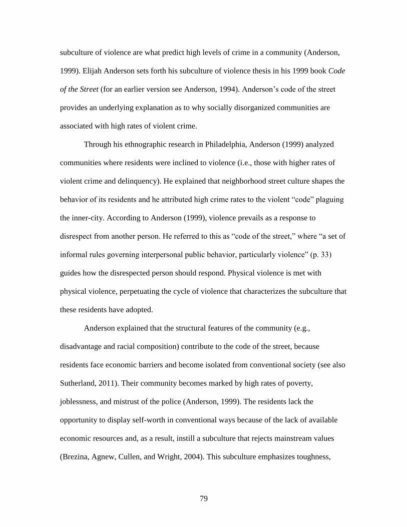
79

subculture of violence are what predict high levels of crime in a community (Anderson,

1999). Elijah Anderson sets forth his subculture of violence thesis in his 1999 book Code

of the Street (for an earlier version see Anderson, 1994). Anderson’s code of the street

provides an underlying explanation as to why socially disorganized communities are

associated with high rates of violent crime.

Through his ethnographic research in Philadelphia, Anderson (1999) analyzed

communities where residents were inclined to violence (i.e., those with higher rates of

violent crime and delinquency). He explained that neighborhood street culture shapes the

behavior of its residents and he attributed high crime rates to the violent “code” plaguing

the inner-city. According to Anderson (1999), violence prevails as a response to

disrespect from another person. He referred to this as “code of the street,” where “a set of

informal rules governing interpersonal public behavior, particularly violence” (p. 33)

guides how the disrespected person should respond. Physical violence is met with

physical violence, perpetuating the cycle of violence that characterizes the subculture that

these residents have adopted.

Anderson explained that the structural features of the community (e.g.,

disadvantage and racial composition) contribute to the code of the street, because

residents face economic barriers and become isolated from conventional society (see also

Sutherland, 2011). Their community becomes marked by high rates of poverty,

joblessness, and mistrust of the police (Anderson, 1999). The residents lack the

opportunity to display self-worth in conventional ways because of the lack of available

economic resources and, as a result, instill a subculture that rejects mainstream values

(Brezina, Agnew, Cullen, and Wright, 2004). This subculture emphasizes toughness,

80

aggression, and revenge, which maintains violent crime in these neighborhoods. Violence

becomes the acceptable means in gaining status, respect, and street credibility

(Wilkinson, 2003; see also Matsueda, Drakulich, and Kubrin, 2006).

Researchers have recognized the value in Anderson’s thesis; the subculture of

violence thesis seems to be prevalent in disorganized communities, which may lead to an

increase in violent crime. In their quantitative study of the applicability of Anderson’s

thesis on youth violent crime, Brezina et al. (2004) reported that, consistent with previous

studies, youth who prescribe to the code of the street are more likely to engage in acts of

violence. Stewart, Schreck, and Simons (2006), however, also reported that youth who

adhere to the violent subculture were more likely to be victims of violence.

Stewart and Simons (2010) analyzed the moderating effects of neighborhood

street culture on individual-level street code values and violence and reported that

neighborhood street culture is a significant predictor of juvenile violence. That is,

residents readily accept the code of the street present within the community, regardless of

individual-level processes. Moreover, Wilkinson (2001) found that young men

committed robberies in an attempt to gain street respect among their peers. Sampson and

Bartusch (1998) suggested that youth adhere to the subculture of violence as a result of

the effects of the inner-city ghetto (e.g., racial isolation and poverty). The structural

features of the community ultimately shape an individual’s perception of the code of the

street.

Concentrated Disadvantage

In his 1987 seminal book The Truly Disadvantaged, William Julius Wilson

evaluated the convergence of race and poverty in the inner-city. Wilson’s most

81

contributing concept to the social disorganization tradition was “concentration effects.”

Sampson and Wilson (1995) explained that concentration effects are a result of the

constraints and lack of opportunity residents of the inner-city face “in terms of access to

jobs and job networks, involvement in quality schools, availability of marriageable

partners, and exposure to conventional role models” (p. 42). This concentration effect

occurred, in part, due to the out-migration of middle-class families, which leaves poor,

African-American communities marked by a number of social problems (Wilson, 1987).

Wilson (1987) argued that several factors interact to create concentration effects,

including: female-headed households with dependent children; the lack of education and

available jobs; the outmigration of white, middle class families; the lack of male role

models; and the lack of transportation out of the urban inner-city. Sampson and Wilson

(1995) stated that patterns of residential inequality faced by African-Americans escalated

social isolation and ecological concentration of the “truly disadvantaged.”

Land, McCall, and Cohen (1990) argued that Wilson’s (1987) concentration

effects set the stage for the methodological association between community-level social

indicators (e.g., family disruption) and economic structure (e.g., poverty) used in

predicting rates of crime. In their examination of the structural covariates of homicide,

Land et al. (1990) used principal components analysis to identify the elements contained

in Wilson’s (1987) concentration effects hypothesis. They concluded that communities

with higher levels of resource deprivation were associated with higher rates of homicide.

More importantly, Land et al.’s (1990) methodological advances allowed researchers to

test the clustering of social and economic elements associated with a disadvantaged

82

community, which helped researchers understand the influence of a community’s

macrostructural characteristics on rates of crime.

According to Clear et al. (2003), concentrated disadvantage “is meant to reflect

the fact that some urban areas are afflicted by multiple problems that place them at a

disadvantage” (p. 43). For example, scholars recognize that with poverty comes a lack of

education and employment opportunities, reliance upon government sources of income,

and family disruption (Clear et al., 2003). Disadvantage is also concentrated in certain

areas, which situates crime in geographic “hot spots” (Sampson, Morenoff, and Gannon-

Rowley, 2002). That is, areas with higher levels of disadvantage display higher levels of

crime.

Today, researchers often measure concentrated disadvantage in terms of an index

of race, class, and other variables (e.g., family disruption and education) (Krivo and

Peterson, 1996; Land et al., 1990; Small and Newman, 2001). Although studies have

differed in their community-level features that constitute the concentrated disadvantage

index, there are a few predictors that are consistent throughout the literature. These

include variables associated with economic disadvantage and family disruption (e.g.,

percent of the population below the poverty line and percent of female-headed

households), as well as a measure of racial composition. Because African-Americans

often live in disadvantaged neighborhoods, researchers use the percent African-American

population as a proxy for determining levels of disadvantage within an area (see e.g.,

Sampson and Raudenbush, 1999). In their meta-analysis of the predictors of crime, Pratt

and Cullen (2005) stated, “Indicators of ‘concentrated disadvantage’ (e.g., racial

heterogeneity, poverty, and family disruption) are among the strongest and most stable

83

predictors” (p. 373). As a result of Wilson’s research on the macrostructural

characteristics that lead to social isolation, measures of community social disorganization

often include a measure of concentrated disadvantage.

3.5 Contemporary Status of Social Disorganization Measures

Contemporary scholars modeling the social disorganization framework have

turned to concentrated disadvantage as one component, yet have maintained that ethnic

heterogeneity and residential instability are important constructs predicting neighborhood

crime rates (see e.g., Sampson et al., 1997). Today, ethnic heterogeneity is measured

using an index of the percent of the population that is Hispanic with percent of the

population that is foreign born; recent literature reports ethnic heterogeneity as

“concentrated immigration” (Sampson et al., 1997).

Early scholars testing concentrated immigration hypothesized that an increase in

immigrant concentration would be associated with an increase in crime because of the

decreased capacity to realize common goals and to achieve informal social controls

(Sampson et al., 1997). Furthermore, immigrants often live in areas marked by

disadvantage and high crime, where they are subjected to the lack of opportunities in

these communities (Bui, 2013). Recently this hypothesis has been rejected and

researchers now suggest that neighborhoods marked by higher concentrated immigration

tend to produce lower rates of crime because immigrants moving into disorganized

communities provide a new sense of organization (Martinez, 2006).

Lee and Martinez (2002) offer an explanation through the immigration

revitalization thesis where “new forms of social organization may include ethnically

situated informal mechanisms of social control and enclave economies that provide stable

84

jobs to co-ethnics” (p. 376). Therefore, heavy immigration in one area may strengthen

social controls and reduce crime in those areas (Lee and Martinez, 2002, 2006; Martinez,

Stowell, and Lee, 2010).

This phenomenon is also apparent in the immigrant paradox literature, where

scholars have suggested that first generation immigrants have better social outcomes (i.e.,

health and education), despite their poor economic situations (Bui, 2013). Suarez-Orozco,

Rhodes, and Milburn (2009) reported a decline in academic achievement and aspirations

in immigrant youth the longer they stayed in the United States. Likewise, Bui (2013)

found the presence of the immigrant paradox in substance use among white, Asian, and

Hispanic youth. That is, recent immigrant youth were socially better off than their non-

immigrant counterparts.

Although ethnic heterogeneity has changed over the years, residential instability

has remained a central component of social disorganization; scholars maintain that

collective efficacy and informal social controls are reduced in unstable environments,

which leads to crime (see Shaw and McKay, 1942). The contemporary measures of

residential instability include an index of the percent of the population living in renter-

occupied homes and the percent of recent (last 5 years) movers (Sampson et al., 1997).

As Brooks-Gunn, Duncan, Klebanov, and Sealand (1993) explained, residential

instability coupled with low rates of home ownership has remained strong correlates of

problem behaviors among residents in changing areas. The majority of empirical

literature suggests that an increase in residential instability is associated with an increase

in crime (e.g., Morenoff et al., 2001; Sampson et al., 1997)

85

The extensions to social disorganization theory have given rise to a renewed

interest in the theory. Scholars agree that several structural dimensions create a setting

favorable for disorganization, which helps explain high crime (Shaw and McKay, 1942;

Sampson et al., 1997). In terms of examining the structural features that create an

environment conducive for crime, Wilson’s (1987) contribution provided explanation for

a link between the macrostructural characteristics of concentrated disadvantage (e.g.,

economic distress, family disruption) and crime. Renewed interest in social

disorganization theory also encouraged researchers to examine the mediating variables

(e.g., social control, collective efficacy) associated with the macrostructural

characteristics of a community and their rates of crime (Bursik and Grasmick, 1993;

Sampson and Groves, 1989).

Researchers often use measures of the structural characteristics of the community

to assess the relationship between a socially disorganized community and crime. For

example, Sampson et al. (1997) examined the link between neighborhood stratification

(concentrated disadvantage, concentrated immigration, and residential instability) and

collective efficacy, in order to predict levels of violence. Using structural measures of

social disorganization, they determined that collective efficacy mediated the relationship

between concentrated disadvantage and residential instability and crime. Therefore, the

structural features of the community created a setting favorable to criminal activity.

Modern testing of social disorganization theory, from a structural standpoint,

includes measures of concentrated disadvantage, concentrated immigration, and

residential instability (e.g., Clear et al., 2003; Morenoff et al., 2001; Sampson et al.,

1997). Together these variables do not necessarily cause a “socially disorganized”

86

community; nevertheless, they remain important concepts for examining environments

conducive to a deficiency in social controls and collective efficacy, leading to increased

criminal behaviors (see e.g., Sampson et al., 1997). Furthermore, scholars have also

argued that areas of extreme disadvantage suffer greater consequences of disorganization

(e.g., higher amounts of crime), because these areas are characterized by severe resource

deprivation (Clear et al., 2003). Often times, these contemporary macrostructural

components are measured and statistically tested individually; the most common current

day hypotheses are that concentrated disadvantage and residential instability have a

positive relationship with crime (e.g., Sampson et al., 1997), while concentrated

immigration has a negative relationship with crime (e.g., Lee and Martinez, 2002).

3.6 Social Disorganization Theory Applied to an Officer’s Use of Discretion

Social disorganization theory was designed by Shaw and McKay (1942) to

explain differences in rates of delinquency based on the macrostructural characteristics of

the community. The theory predicts that people’s behavior (whether criminal or

legitimate) become a reflection of the community in which they reside (or spend a large

portion of time) (see e.g., Sampson et al., 1997). Sampson (2002) states, “crimes are not

randomly distributed in space. Rather, they are disproportionately concentrated in certain

neighborhoods” (p. 243). Disorganized neighborhoods are subjected to higher amounts of

crime because residents lack the informal social controls necessary to regulate criminal

conduct (Bursik, 1988). Researchers have argued that community context not only shapes

the residents’ behaviors, but may also influence an officer’s decision-making behaviors

(e.g., Smith, 1986; Terrill and Reisig, 2003). Three theoretical associations between a

community’s level of social disorganization, normally predicting crime within a

87

community, and an officer’s decision-making can be reasoned (see Kane, 2002; Sun et

al., 2008).

The first theoretical connection is grounded in the basic relationship between the

macrostructural characteristics (e.g., concentrated disadvantage) of a community and its

crime rates. In its simplest form, the structural features that generate a socially

disorganized neighborhood lead to higher rates of crime, compared to an affluent

neighborhood (Shaw and McKay, 1942). Recent theoretical advances have shown a

positive relationship between the amount of concentrated disadvantage and residential

instability and crime (Krivo and Peterson, 1996); it is argued that communities with

higher levels of disorganization naturally have higher rates of crime (see Wilson, 1987).

Police behavior, then, becomes driven by the amount of criminal activity within a

community (Terrill and Reisig, 2003).

An officer’s goal is to maintain order and uphold the law (National Research

Council, 2004). As Sampson (2002) claimed, crimes are concentrated in certain areas; so,

it can intuitively be argued that police will also be concentrated in certain areas. For

example, rates of search and arrest will be more common in a disadvantaged and high

crime neighborhood, compared to an affluent neighborhood, simply because of the sheer

amount of police activity in those areas (see e.g., Smith, 1986). Police have a greater

presence in these communities in order to reduce criminal behaviors; Fagan (2012)

reported higher rates of stops in areas with greater police presence, which is expected.

Moreover, in disadvantaged communities, where crime is high, police are

(hypothetically) inclined to respond more coercively (e.g., Terrill and Reisig, 2003) to

protect themselves and others from victimization. Because of the high amount of criminal

88

activity within a disadvantaged community, an officer is at a greater risk of facing a

dangerous situation. An officer’s decision-making becomes a product of his perception of

risk; an officer is more likely to act coercively toward a suspect (e.g., search) when the

risk of danger is greater. Concentrated disadvantage, therefore, makes the relationship

between the reason for the stop and the coercive action taken during the stop more

meaningful. That is, concentrated disadvantage may encourage the officer to take a more

coercive approach when a suspect is stopped. Furthermore, these effects will be

pronounced in areas of extreme disadvantage, where crime and the officer’s perception of

risk are maximized.

Second, scholars have reasoned that a disorganized neighborhood is one marked

by inefficient informal social controls used to regulate criminal behavior (Bursik and

Grasmick, 1993). In disorganized neighborhoods, or those with a deficiency in friendship

networks and collective efficacy (see Sampson et al., 1997), it becomes increasingly

more difficult to control criminal behaviors through informal means. In these

communities, the police are expected to fill in as representatives of control (Clear et al.,

2003). This is what Bursik and Grasmick’s (1993) systemic model explained. Their

model suggested a negative relationship between relational networks (e.g., family groups)

and formal social controls, and a negative relationship between formal controls and

crime. That is, in communities where relational networks fail to regulate criminal

conduct, formal controls must step in to regulate criminal conduct.

Black (1976) recognizes that the use of the law varies inversely with informal

social control. Black explained that when nonlegal authority (e.g., parental control of

juveniles) is strong, little formal recourse (e.g., the law) is used. He stated, “Law is

89

stronger where other social control is weaker” (Black, 1976, p. 107). This would then

suggest that officers respond more coercively to crimes occurring in areas with a

deficiency in informal social controls. For example, Wilson (1978) stated that police

officers were more likely to arrest and use physical force in areas that were believed to

have weakened community or familial norms. This link suggests that an officer would be

more inclined to act coercively in areas that do not have the means necessary to deal with

criminal conduct. As agents of formal social control, the police are expected to act as

mechanisms of control in the communities where residents lack the informal social

controls necessary to regulate criminal behaviors (see also Rose and Clear, 1998).

Further, Anderson (1999) argued that residents of disadvantaged communities are

more likely to adopt a violent subculture because they are isolated from the norms and

values of conventional society. In these communities that lack the conventional ways of

controlling crime (e.g., informal social controls), police respond coercively to control

criminal behaviors. Police use of coercion will be higher in disadvantaged communities,

and even more pronounced in areas of extreme disadvantage, whose residents have

adopted the subculture of violence; police will be more inclined to respond in a way that

is normal to the deviant subculture (e.g., use of force) (Kania and Mackey, 1977).

Through the lack of informal social controls and the residents’ adherence to the

subculture of violence, concentrated disadvantage, again, makes the relationship between

a suspect being stopped and coercive action more meaningful.

An alternative hypothesis is that officers who work in areas marked by low

amounts of informal social controls may be less likely to act coercively during a PCI.

Khruakham and Hoover (2012), for example, reported that police use less coercion in

90

disadvantaged and high crime neighborhoods. A deficiency in informal social controls in

these areas may, inadvertently, cause a breakdown in formal social controls, which can be

explained by Klinger’s (1997) ecological theory of police behavior. Only the most

serious crimes will be handled coercively because police feel cynical towards residents,

officers see deviance as more accepting in these communities, and police are too busy

with heavy workloads in these areas to deal with lower level offenses (Klinger, 1997).

Police become cynical and desensitized to crime occurring in these areas, often

perceiving victims as less deserving (Sobol et al., 2013). In communities marked by low

informal social controls police often see their efforts as wasteful and, therefore, reduce

their coercive responses to criminal conduct. In this theoretical connection, concentrated

disadvantage has a weakening influence on the relationship between a stop and coercive

action. That is, concentrated disadvantage may encourage the officer to take a less

coercive approach when a suspect is stopped, with these effects exacerbated in extremely

disadvantaged areas.

In summary, the first theoretical connection lies in the simple link between

disadvantage and high crime leading to an increase in police activity and risk of

victimization. Areas with greater police activity and a greater risk of danger will naturally

have higher amounts of police coercion (e.g., search and arrest rates) (e.g., Terrill and

Reisig, 2003). The second and third theoretical connections would argue that police

decision-making becomes molded by the intervening mechanisms at play (e.g., informal

social controls and subculture) in a socially disorganized community. The second

connection is that police use coercion more frequently to act as a mechanism of control,

where informal social controls fail and a subculture of violence prevails (e.g., Clear et al.,

91

2003). The third connection is that police use coercion less frequently in communities

lacking informal social control because police perceive their efforts to be wasteful and

victims as less deserving (e.g., Klinger, 1997). Literature examining police decision-

making in terms of these theoretical connections, however, remains scarce.

92

CHAPTER 4

DATA AND METHODS

This dissertation explores the role of neighborhood-level disorganization on

police decision-making. In 1997, Klinger proposed an ecological theory to explain police

behavior, stating that police decision-making is driven by the features of the community.

Social disorganization theory may be used to explain an officer’s decision-making within

a community, though prior literature is quite scant (for an exception see Kane, 2002).

Furthermore, Terrill and Reisig (2003) noted that previous literature examining

neighborhood-level factors on police decision-making has relied upon statistical

techniques not designed to analyze nested data (i.e., PCIs nested within neighborhoods).

Multilevel modeling will provide insight into how contemporary measures of social

disorganization theory account for an officer’s decision-making during a PCI. Multilevel

modeling will also allow for a cross-sectional analysis of the moderating effects of

concentrated disadvantage, as well as extreme disadvantage, on the relationship between

stop predictors and an officer’s use of coercive actions.

A socially disorganized or disadvantaged neighborhood may influence an

officer’s decision to use coercion during a stop, but there may also be an interaction

effect between neighborhoods and the reason for the stop and an officer’s decision to act

coercively. Prior research has reported that neighborhood disadvantage shapes an

officer’s use of discretion (e.g., Terrill and Reisig, 2003). Concentrated disadvantage,

however, may also make the relationship between a stop and coercive action more

93

understandable. That is, officers may become more likely to respond in ways consistent

with the features of the environment – high crime, lack of informal social controls, and

the presence of a violent subculture. These effects are expected to be more pronounced in

areas of extreme disadvantage, where concentrated disadvantage and high crime is

prominent. Analyses using data from the NYPD will provide answers to two main

questions:

(1) Does neighborhood disorganization play a role in an officer’s decision to

frisk, search, use force against, or arrest a suspect?


between predictors of a stop and an officer’s decision to frisk, search, use


4.1 Sample

The data set consists of police recorded stops of people in New York City along

with information regarding neighborhood structural and demographic characteristics. The

New York Police Department Stop, Question, and Frisk Database, 2011 (NYPD SQF)

serves as the foundation of the data set. The NYPD SQF contains all reported street

encounters between NYPD officers and citizens resulting in completion of a Unified

Form 250 (UF-250) report during 2011.8 As previously explained, a UF-250 report gives

details of each street stop between an officer and citizen, as recorded by the reporting

officer. The measures used from this database are discussed below.

New York City neighborhood (tract) data were obtained from the U.S. Census

Bureau, 2010 and was subsequently combined with data from the NYPD SQF database.

8 It is important to note that the NYPD SQF does not contain information from traffic

stops and only includes stops made during street encounters.

94

The data collected from the U.S. Census Bureau included information from census tracts,

which are frequently used to approximate a neighborhood context. Fagan (2012)

explained that census tracts are often used in research examining the effects of small

areas on crime and enforcement, and are well-known boundaries for such studies (see

also Krivo and Peterson, 1996).

In order for the NYPD SQF database to be combined with census tract structural

and demographic characteristics, geocoding procedures had to be utilized. The NYPD

SQF database contains individual stop events listed as x, y coordinates. Each stop event

was geocoded using ArcGIS version 10.2 to allow the stop incident to be mapped into a

New York City census tract boundary (neighborhood). The final sample consists of

654,485 stop incidents nested within 2,114 tracts.9

Weaknesses of UF-250 Reports

Although the stop and frisk policy mandates the completion of UF-250 form

under certain circumstances of a stop, it cannot be fully verified that the officer followed

proper procedures. In the 1999 investigation of the NYPD’s use of the stop and frisk

policy, the officers selected for interviews reported that even those stops that mandated a

completion of a UF-250 report were, at times, not completed; the officers did not provide

reasons or the degree of the underreporting (Spitzer, 1999). Although stop and frisk

reporting procedures are much more rigorous ten years later, it is possible that officers

9 Seven percent of stop incidents were dropped from the data set due to missing x,y

coordinates and .26% of the stops did not fall within a New York City census tract. A

total of 52 census tracts had no households and 47 of the 52 had no population statistics,

which also were dropped from the data set. Further, 7 census tracts had no stops

occurring within them, and were therefore not included in the analyses.

95

still do not follow proper guidelines outlined by the NYPD Patrol Guide. In 2007,

Ridgeway questioned NYPD officers about the stop and frisk policy. Ridgeway reported

that officers freshly out of the academy (one year or less) seemed to lack knowledge on

proper stop and frisk procedures, stating:

While it appears that some of the newest members of the force are uncertain about

how to document street encounters properly, this is not entirely surprising. The

interviewed are working essentially alone in extremely busy areas and are

learning to put their academy training into practice. Officers interviewed who had

a year or more on the job knew the policies and the practices well and expressed

no confusion on the issue. (p. 3-4).

The NYPD currently has several layers of auditing checks to ensure police

officers are properly reporting stops (Ridgeway, 2007). Once the officer fills out the UF-

250 report, it is reviewed by a supervisor, then screened by data entry staff, and then is

reviewed by the integrity control officer (ICO) to assess any incongruences that may be

present between the initial stop and the coercive action taken by the officer, in particular

arrests. Lastly, the NYPD’s Quality Assurance Division reviews the ICO’s audits,

randomly collecting UF-250 reports from each command to ensure proper procedures are

being followed (Ridgeway, 2007).

Unfortunately there is no auditing process to ensure the officers are filling out the

UF-250 report for every mandated PCI. John Timoney (in Trone, 2010) postulated that

when an arrest occurs, officers most likely fill out the required arrest forms, but most

likely do not fill out the UF-250 documenting the stop, losing the detailed information

between the stop and the arrest. However, in one eight-hour shift observation of PCIs and

96

monitored radio communication, Ridgeway (2007) reported that officers did submit all

mandated UF-250 reports.

Although there are audits and quality checks of the UF-250 reports, the officer

could have misreported (either accidentally or purposefully) what occurred during the

stop, potentially going unnoticed by auditors. For example, the officer could have

checked the wrong box that reports the circumstance that lead to the stop or checked the

wrong box for the coercive activity that occurred during the stop. The officer could also

have not remembered the exact reason for the stop or that he used multiple forms of

coercive activity during the stop. If the officer searched the suspect, along with enacting a

type of force and arresting the suspect and only checked the boxes for use of force and

arrest, then, in this case, would have inaccurately reported.

Further, an officer’s use of discretion (e.g., whether or not to arrest the suspect

when a small amount of illegal drugs were found on their person) may have interfered

with the accuracy of the data. A police sergeant was quoted, “’I’m wondering...whether

contraband and possibly weapons have been found, but the officer utilizing their

discretion has not made an arrest; and whether that’s skewing the data somehow’”

(Trone, 2010, p.8). Regardless of these potential limitations, the UF-250 reports remain

the most valuable data source for purposes of the current analysis.

In terms of the amount of stops, Ridgeway (2007) notes that a certain number of

officers may be over- or under-representing the number of stops that are occurring in

New York City. In RAND’s examination of 2006 NYPD stops it was reported that “…the

analysis flagged 0.5 percent of the 2,756 NYPD officers most active in pedestrian-stop

activity. Those 2,756 most active officers, about 7 percent of the total number of officers,

97

accounted for 54 percent of the total number of 2006 stops” (Ridgeway, 2007).

Regrettably, the current data does not allow for such an analysis; there is no officer

identification number associated with the individual stop events to examine if a few

officers are making up the majority of stops.10

This same phenomenon may also occur on

the suspect side. That is, a person may have been stopped several times, but again, the

current data do not allow for such an analysis.

Another weakness to the data is the way the UF-250 report is formatted; the

variables included in the report are not clearly defined. The data mostly consists of

dichotomies (yes and no) and do not provide significant detail into officer responses on

the UF-250. For example, the stop predictor furtive movements does not specifically

explain the type of movements the suspect was performing, only that the officer stopped

(or did not stop) the person for this reason. Furtive movements remains one of the most

commonly used stop predictor (occurring in 51% of recorded stops) and is argued by

Jones-Brown, Gill, and Trone (2010) to be “a term that is highly ambiguous and

undefined” (p. 22). A retired NYPD officer was quoted saying, “Is that furtive

movements like I’m looking over my shoulder because I don’t want to get mugged in my

neighborhood?...Furtive movements right there tells me that cops are out there winging it

a bit” (Trone, 2010, p.11).

Furthermore, there are “other” categories on the UF-250 report that offer no

detailed description. The outcome variable use of force has an “other” category that the

10 If data permitted, a within-officer examination of stops incidents and the coercive

activity used during the stop could have provided insight into officer proactivity within

certain neighborhoods.

98

officer may have marked on the UF-250 report. It is unclear what “other” methods of

force the officer may have utilized; only logical inferences may be made. For example,

the officer using his hands against the suspect was listed as an option in the UF-250

report, but the officer kicking the suspect was not included in the report. It can be

logically inferred that an officer may have chosen the “other” category in these situations.

Likewise, the individual-level stop predictors had an “other reasonable suspicion of

criminal activity” category that also did not provide explanation for the reason of the

stop. Again it can be inferred that an officer may check this box if the reason the officer

stopped the suspect was not otherwise listed on the UF-250 report.

Measures

This study uses data collected from the NYPD UF-250 reports and from New

York City census tracts. There are five main types of police coercive responses included

in the UF-250 reports (no coercive action/stop only, frisk, search, use of force, and

arrest). It is unlikely that a single method of estimation will properly capture the full

picture behind factors influencing an officer’s decision to use coercion. As such, the

outcome variables used in this analysis are measured three ways: (1) as a dichotomy of

each coercive response occurring or not occurring during the stop (2) on a continuum of

coercive action and (3) using the highest level of coercive action that occurred during the

stop (see also Klinger’s 1995 and Garner and Maxwell’s 1999 police use of force

measures). Table 4.1 describes the outcome measures used in the current analysis.

Dichotomous outcomes.

The first method that will be employed is analyzing each coercive action as a

separate dichotomy (e.g., Garner and Maxwell, 1999). The first outcome, No Coercive

99

Table 4.1 Description of outcome measures

Variable Mean SD Minimum-Maximum

Dichotomous Outcomes

No coercive action/stop only .42 -- 0-1

Frisk .56 -- 0-1

Search .09 -- 0-1

Use of force .20 -- 0-1

Arrest .06 -- 0-1

Coercive Action Continuum 3.01 3.09 1-16

1. No coercive action/stop only .42 -- 0-1

2. Frisk only .31 -- 0-1

3. Search only .00 -- 0-1

4. Frisk and search .03 -- 0-1

5. Use of force only .01 -- 0-1

6. Frisk and use of force .15 -- 0-1

7. Search and use of force .00 -- 0-1

8. Frisk, search, and use of force .02 -- 0-1

9. Arrest only .01 -- 0-1

10. Frisk and arrest .01 -- 0-1

11. Search and arrest .00 -- 0-1

12. Frisk, search, and arrest .02 -- 0-1

13. Use of force and arrest .00 -- 0-1

14. Frisk, use of force, and arrest .00 -- 0-1

15. Search, use of force, and arrest .00 -- 0-1

16. Frisk, search, use of force, and arrest .01 -- 0-1

Highest Level of Coercion Used 2.15 1.30 1-5

1. No coercive action/stop only .42 -- 0-1

2. Frisk .31 -- 0-1

3. Search .03 -- 0-1

4. Use of force .18 -- 0-1

5. Arrest .06 -- 0-1

Action, means that the suspect was stopped only; no other action was taken against the

suspect (n=274,463). The second outcome, Frisk, represents whether or not the suspect

was frisked, which occurs when the officer “pats down” or moves his or her hands

quickly over the person’s body in order to detect weapons or other illegal contraband

(Harris, 1994a). In 56% of the recorded stops, the suspect was frisked (n=365,206). The

third outcome of interest, Search, signifies whether or not the officer investigated the

suspect’s possessions (e.g., his bag or his pants pockets) (Harris, 1994a). In 9% of

recorded stops the suspect was searched (n=55,668). The fourth outcome variable

analyzed, Use of force, denotes whether or not force was used against the suspect. Use of

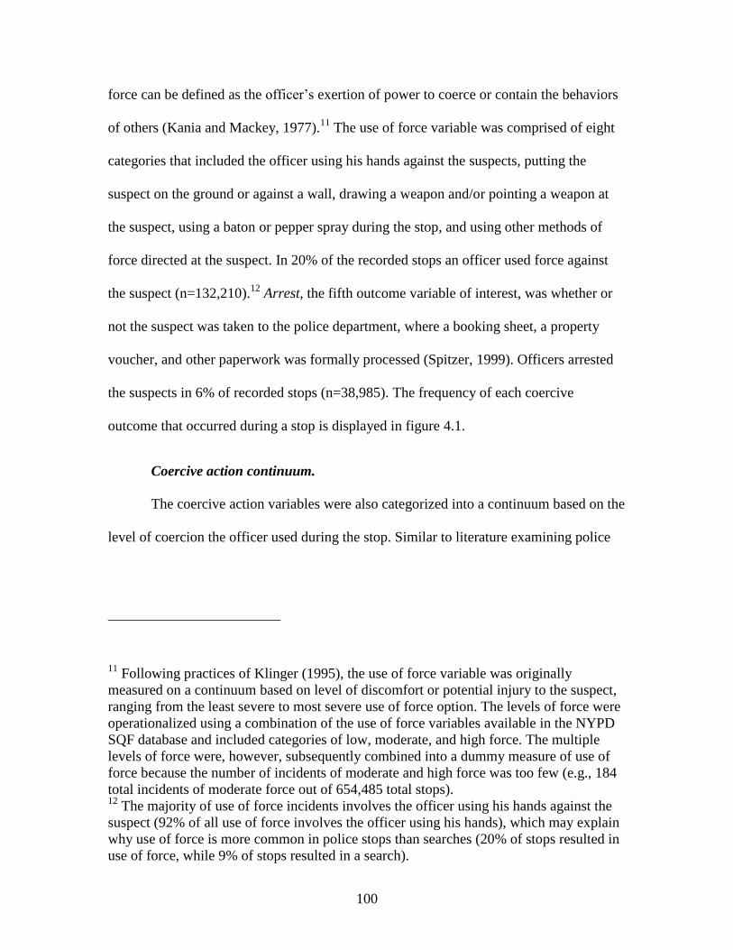
100

force can be defined as the officer’s exertion of power to coerce or contain the behaviors

of others (Kania and Mackey, 1977).11

The use of force variable was comprised of eight

categories that included the officer using his hands against the suspects, putting the

suspect on the ground or against a wall, drawing a weapon and/or pointing a weapon at

the suspect, using a baton or pepper spray during the stop, and using other methods of

force directed at the suspect. In 20% of the recorded stops an officer used force against

the suspect (n=132,210).12

Arrest, the fifth outcome variable of interest, was whether or

not the suspect was taken to the police department, where a booking sheet, a property

voucher, and other paperwork was formally processed (Spitzer, 1999). Officers arrested

the suspects in 6% of recorded stops (n=38,985). The frequency of each coercive

outcome that occurred during a stop is displayed in figure 4.1.

Coercive action continuum.

The coercive action variables were also categorized into a continuum based on the

level of coercion the officer used during the stop. Similar to literature examining police

11 Following practices of Klinger (1995), the use of force variable was originally

measured on a continuum based on level of discomfort or potential injury to the suspect,

ranging from the least severe to most severe use of force option. The levels of force were

operationalized using a combination of the use of force variables available in the NYPD

SQF database and included categories of low, moderate, and high force. The multiple

levels of force were, however, subsequently combined into a dummy measure of use of

force because the number of incidents of moderate and high force was too few (e.g., 184

total incidents of moderate force out of 654,485 total stops). 12

The majority of use of force incidents involves the officer using his hands against the

suspect (92% of all use of force involves the officer using his hands), which may explain

why use of force is more common in police stops than searches (20% of stops resulted in

use of force, while 9% of stops resulted in a search).

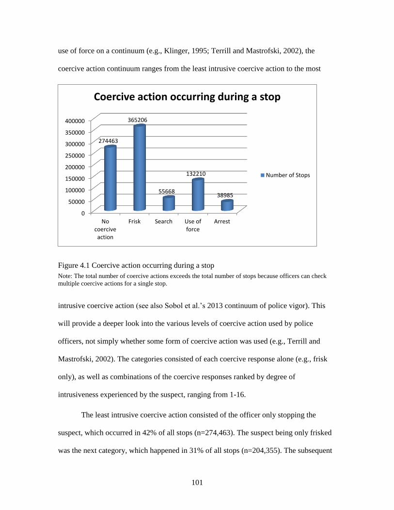
101

use of force on a continuum (e.g., Klinger, 1995; Terrill and Mastrofski, 2002), the

coercive action continuum ranges from the least intrusive coercive action to the most

Figure 4.1 Coercive action occurring during a stop

Note: The total number of coercive actions exceeds the total number of stops because officers can check

multiple coercive actions for a single stop.

intrusive coercive action (see also Sobol et al.’s 2013 continuum of police vigor). This

will provide a deeper look into the various levels of coercive action used by police

officers, not simply whether some form of coercive action was used (e.g., Terrill and

Mastrofski, 2002). The categories consisted of each coercive response alone (e.g., frisk

only), as well as combinations of the coercive responses ranked by degree of

intrusiveness experienced by the suspect, ranging from 1-16.

The least intrusive coercive action consisted of the officer only stopping the

suspect, which occurred in 42% of all stops (n=274,463). The suspect being only frisked

was the next category, which happened in 31% of all stops (n=204,355). The subsequent

0

50000

100000

150000

200000

250000

300000

350000

400000

Nocoerciveaction

Frisk Search Use offorce

Arrest

274463

365206

55668

132210

38985

Coercive action occurring during a stop

Number of Stops

102

category, the suspect was only searched, occurred in .0006% of all stops (n=412). A

combination of the suspect being frisked and searched was the next category of

intrusiveness, which occurred in 3% of all stops (n=16,789). Following, the officer using

force against the suspect happened in 1% of all stops (n=8,240). Frisk combined with use

of force (15% of all stops; n=97,443), search combined with use of force (.0002% of all

stops; n=128), and frisk combined with search and use of force (2% of all stops;

n=13,670) were the next three categories on the continuum.

The next category along the continuum consisted of the suspect being only

arrested, which occurred in 1% of all stops (n=3,797). Then, the suspect being frisked and

arrested (1% of all stops; n=7,054), the suspect being searched and arrested (.002% of all

stops; n=1,425), and the suspect being frisked, searched, and arrested (2% of all stops;

n=13,979) were the next three categories on the continuum. Following, the suspect

having force used against him and being arrested accounted for .0006% of all stops

(n=418). The next category was the suspect being frisked, force used against him, and he

was arrested, which occurred in .005% of all stops (n=3,047). After this category, the

suspect was searched, force was used against him, and he was arrested, which happened

in .0006% of all stops (n=396). Lastly, the most intrusive coercive action used, is all

types of coercion combined. The suspect was frisked, searched, force was used against

him, and he was arrested in this category, which occurred in 1% of all stops (n=8,869).

Figure 4.2 displays the frequency of the coercive action continuum categories.

Highest level of coercion used

In Klinger’s (1995) observational study of Metropolitan Dade County Police

Department he suggested multiple methods for measuring levels of police use of force.

103

Figure 4.2 Coercive action continuum

Because multiple methods of force may be used in one PCI (e.g., an officer may use

verbal commands and his baton), Klinger proposed an examination of the highest level of

force used in each incident to explore this dynamic (see also Paoline and Terrill, 2007;

Terrill and Reisig, 2003). The data for this dissertation also follow this pattern; an officer

may have used multiple forms of coercive action in a stop (e.g., a suspect may have been

frisked and arrested). Therefore, I also examine the highest level of coercion used in each

stop performed by the NYPD.

0

50000

100000

150000

200000

250000

300000

No

co

erci

ve a

ctio

n/S

top

on

ly

Fris

k o

nly

Sear

ch o

nly

Fris

k an

d s

earc

h

Use

of

forc

e

Fris

k an

d u

se o

f fo

rce

Sear

ch a

nd

use

of

forc

e

Fris

k, s

ear

ch, a

nd

use

of

forc

e

Arr

est

Fris

k an

d a

rre

st

Sear

ch a

nd

arr

est

Fris

k, s

ear

ch, a

nd

arr

est

Use

of

forc

e a

nd

arr

est

Fris

k, u

se o

f fo

rce

, an

d a

rres

t

Sear

ch, u

se o

f fo

rce,

an

d a

rre

st

Fris

k, s

ear

ch, u

se o

f fo

rce,

an

d…

274463

204355

412 16789

8240

97443

128 13670

3797 7054 1425 13979

418 3047 396 8869

Coercive action continuum

Number of stops

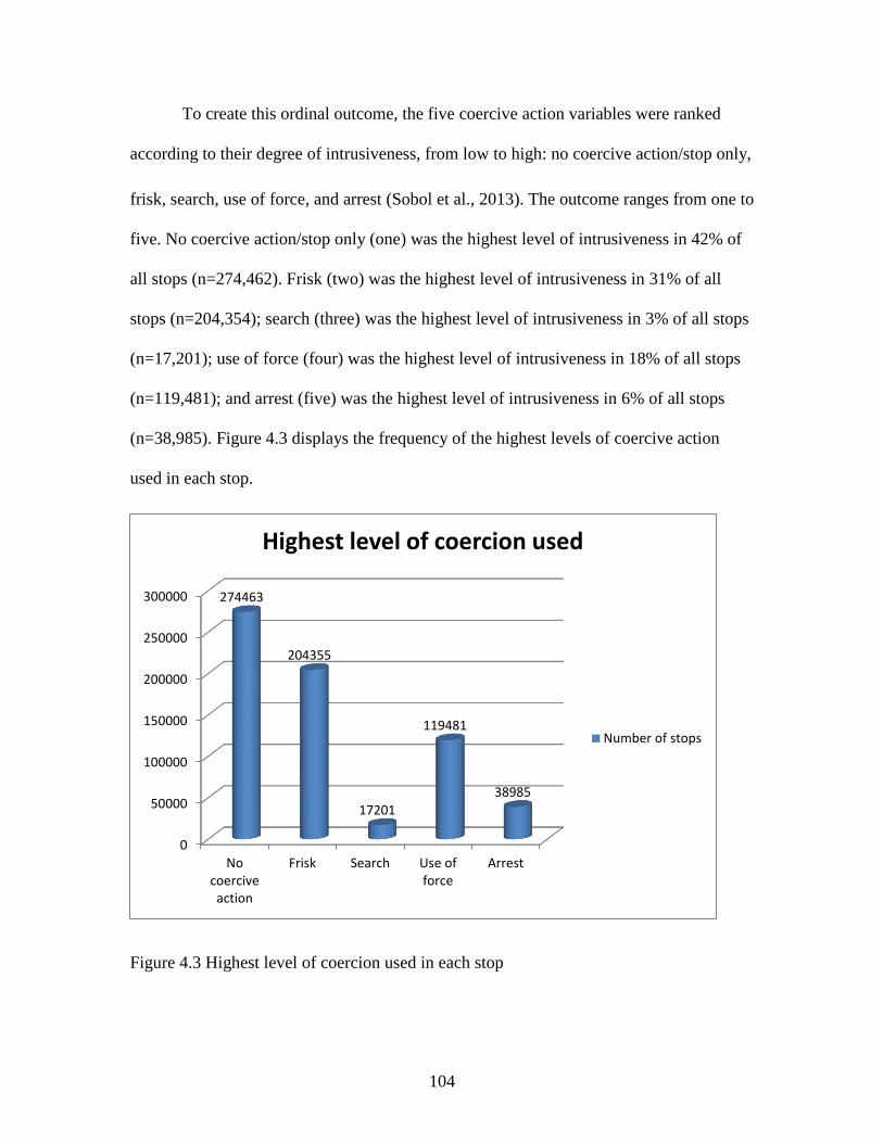
104

To create this ordinal outcome, the five coercive action variables were ranked

according to their degree of intrusiveness, from low to high: no coercive action/stop only,

frisk, search, use of force, and arrest (Sobol et al., 2013). The outcome ranges from one to

five. No coercive action/stop only (one) was the highest level of intrusiveness in 42% of

all stops (n=274,462). Frisk (two) was the highest level of intrusiveness in 31% of all

stops (n=204,354); search (three) was the highest level of intrusiveness in 3% of all stops

(n=17,201); use of force (four) was the highest level of intrusiveness in 18% of all stops

(n=119,481); and arrest (five) was the highest level of intrusiveness in 6% of all stops

(n=38,985). Figure 4.3 displays the frequency of the highest levels of coercive action

used in each stop.

Figure 4.3 Highest level of coercion used in each stop

0

50000

100000

150000

200000

250000

300000

Nocoerciveaction

Frisk Search Use offorce

Arrest

274463

204355

17201

119481

38985

Highest level of coercion used

Number of stops

105

Individual-Level Measures

The predictor variables included both individual- and neighborhood-level

measures and are described in Table 4.2. For the individual-level variables, several stop

Table 4.2 Description of Independent Measures

Variable Mean SD Minimum-Maximum

Stop-level reason for the stop variables

Carrying suspicious object .02 -- 0-1

Fits a relevant description .16 -- 0-1

Casing a victim or location .32 -- 0-1

Acting as a lookout .18 -- 0-1

Wearing clothes commonly used in a crime .05 -- 0-1

Actions indicative of a drug transaction .07 -- 0-1

Furtive movements .51 -- 0-1

Actions of engaging in violent crime .10 -- 0-1

Suspicious bulge .08 -- 0-1

Other reasonable suspicion of criminal activity .17 -- 0-1

Stop-level control variables

Area under investigation .14 -- 0-1

Area has a high crime incidence .60 -- 0-1

Time of day fits crime incidence .42 -- 0-1

N1 = 654,485

Neighborhood-level variables

Concentrated disadvantage 0.0 1.0 -1.57 to 6.36

Extreme disadvantage .10 .30 0 to 1

Concentrated immigration 0.0 1.0 -2.37 to 4.77

Percent recent movers 10.95 7.19 0 to 60.82

Percent renters 62.48 25.96 0 to 100

Percent African-American 26.49 31.46 0 to 100

Percent Hispanic 26.22 23.20 0 to 100

Neighborhood-level control variables

Manhattan .13 -- 0 to 1

Bronx .16 -- 0 to 1

Brooklyn .35 -- 0 to 1

Queens .30 -- 0 to 1

Staten Island .05 -- 0 to 1

N2 = 2,114

predictors, or reason the officer stopped the citizen, were included in the analysis. Figure

4.4 displays the frequency of each stop predictor that led to the officer stopping the

person; an officer may have checked more than one reason for the stop on the UF-250

report. Carrying a suspicious object represents whether or not the suspect was carrying an

object in plain view that could potentially be used in commission of a crime (e.g, slim

106

jim/pry bar). In 2% of all stops the officer believed the suspect was carrying a suspicious

object (n=13,089). Fits a relevant description signifies that the officer believed the

suspect fit a description of someone who was previously involved in criminal activity.

Figure 4.4. Reason for the stop

Note: The total number of reasons for the stop exceeds the total number of stops because officers can check

multiple reasons for a single stop.

An officer’s account of the basis for fitting a relevant description is described in Spitzer

(1999), “At TPO [time and place of occurrence] male was person who fit description of

person wanted for GLA [grand larceny auto] in 072 pct. log…upon approach male

0

50000

100000

150000

200000

250000

300000

350000

13089

104717

209435

117807

32724 45813

333787

65448 52358

111262

Reason for the stop

Number of Stops

107

discarded small coin roller which contained 5 bags of alleged crack” (p. 137). The

suspect being stopped for fitting a relevant description occurred in 16% of all stops

(n=104,717).

Casing a victim or location denotes that the officer believed the suspect displayed

actions of casing a victim or location, which occurred in 32% of all stops (n=209,435).

Acting as a lookout represents that the officer believed the suspect displayed actions of

assisting in criminal activity. The suspect being stopped for acting as a lookout occurred

in 18% of all stops (n=117,807). Wearing clothes commonly used in a crime signifies that

the officer believed that the suspect intended to engage in criminal activity, based on his

or her attire; this occurred in 5% of all stops (n=32,724). Actions indicative of a drug

transaction symbolizes that the officer believed the suspect was displaying actions

commonly used in drug deals. The officer stopped the person based on these actions in

7% of all recorded stops (n=45,813). Furtive movements means that the officer believed

the suspect was demonstrating secretive or sneaky movements, which occurred in 51% of

the recorded stops (n=333,787). Over the years of collected UF-250 data furtive

movements continues to be the most frequently chosen reason for the officer making the

stop.

Actions of engaging in a violent crime denotes that the officer believed the

suspect was currently involved in violent criminal activity, which was observed in 10%

of the recorded stops (n=65,448). Suspicious bulge represents that the officer saw a

prominent object on the suspect that could potentially be dangerous. An officer’s account

stated, “Observed person with large bulge in front right coat, thought to be a weapon”

(Spitzer, 1999, p. 138). Suspicious bulge made up 8% of recorded stops (n=52,358).

108

Lastly, other reasonable suspicion of engaging in criminal activity is when the officer

believed the suspect was involved in criminal activity not previously listed in the UF-250

report’s reasons for the stop; this occurred in 17% of the recorded stops (n=111,262).

Neighborhood-Level Measures

The neighborhood-level variables included measures of disorganization within

New York City neighborhoods, all retrieved from the U.S. Census Bureau’s American

Fact Finder. A principle components analysis of seven neighborhood-level indicators

revealed a two factor solution explaining 69% of the variation in the indicators (Kaiser-

Meyer-Olkin Measure of Sampling Adequacy = .74). The factors represent the structural

features of the neighborhood, namely, concentrated disadvantage and concentrated

immigration (see e.g., Morenoff et al., 2001; Sampson et al., 1997). Concentrated

disadvantage (Eigenvalue = 1.66) is comprised of the following: percent of civilian

working age population unemployed; percent female-headed households; percent of

population receiving public assistance; percent of population age 16-19 who dropped out

of high school; and percent of population living in poverty. Concentrated immigration

(Eigenvalue = 3.15) reflects the percent of population that is Asian and percent of

population foreign born. This measure does not follow the usual pattern found in prior

literature examining concentrated immigration, which is often comprised of the percent

of population that is foreign born and the percent of population that is Hispanic (e.g.,

Sampson et al., 1997). This concentrated immigration variable may be explained by the

109

increase in Asian immigration in New York City in the past few years.13

According to the

U.S. Census Bureau (2011), the sub-groups of all Asian immigrants have progressively

inclined from year 2000 to 2010, while sub-groups of Hispanic population have either

declined or stayed steady during this time in New York City. For example, from year

2000 to 2010, the Dominican immigrant population changed to a decrease of 11.2%,

while the Chinese immigrant population changed to a 34% increase in New York City

(U.S. Census Bureau, 2011). This dramatic increase in Asian immigrants in New York

City may explain why the percent of the population that is foreign born loads on the same

factor as the percent of the population that is Asian.

Variables that were also included in the analysis were extreme disadvantage,

percent recent movers, percent renters, percent African-American, and percent Hispanic.

Extreme disadvantage represents the worst off neighborhoods within New York City.

Recall that the effects of disorganization and high crime may be exacerbated in areas of

extreme disadvantage (Clear et al., 2003), with police potentially more (or less) inclined

to respond coercively in these areas. The extreme disadvantage measure was created

using the top 10% of the concentrated disadvantage index. Percent recent movers and

percent renters are variables used to approximate the residential instability component of

social disorganization.14

In the principal components analysis, percent African-American

13 Immigrants from the Dominican Republic made up 12.4% of the foreign born

population, while Chinese immigrants made up 11.4% of the foreign born population in

New York City (U.S. Census Bureau, 2011). 14

Residential instability customarily consists of two variables (1) percent of the

population that has moved within the past 5 years and (2) percent of households renter-

occupied. In New York City, the percent of renter-occupied households does not load

with the other measure of residential instability. It seems that because households within

110

did not load with the variables of concentrated disadvantage, as in prior literature, and is

included in the analysis as a separate variable. Likewise, percent Hispanic is also

included as a separate variable in analyses.

Finally, control variables were used to help avoid misspecification of the risk of

being stopped by the police in a particular neighborhood. These measures were collected

form the UF-250 reports and included: Ongoing investigation, which denotes that the

area is under investigation of crime patterns (e.g., robbery pattern); Time of day fits crime

incidence, which represents whether or not the time of the day, the day of the week, or

the season corresponds to reports of criminal activity; and area has high crime incidence

signifies that the area has high reports of offenses of the type under investigation.

Another control variable used in the analysis is the New York City borough in

which the stop occurred. Borough is included as a control to account for variation across

boroughs that are not accounted for by census tract data (e.g., differences in rates of

crime, department policies, recent political agendas, etc.; see e.g., Fagan, 2012). Staten

Island, because of its dissimilar rates of NYPD stops, is used as the reference category in

this analysis. In 2011 Staten Island reported 26,310 stops while the other boroughs

(Brooklyn, Bronx, Manhattan, and Queens) had over 125,000 stops occurring within their

boundaries.15

New York City are largely renter-occupied, it does not necessarily denote that the

neighborhood is marked by transiency. Therefore, percent of the population that has

moved in the past one year and percent renters are included separately to represent

residential instability. The past one year, as opposed to the past 5 years, was believed to

be a better indicator of recent residential instability within a neighborhood. 15

Brooklyn reported 221,975 stops, Bronx reported 127,608 stops, Manhattan reported

133,929 stops, and Queens reported 144,673 stops.

111

4.2 Analytic Strategy

Multilevel modeling techniques using HLM 7.01 software were used to

accommodate the hierarchical structure of the nested data (individual stop events nested

within neighborhoods). First, diagnostic tests for multicollinearity were conducted using

linear regression modeling and revealed no issues (all VIFs were ≤ 1.33 and condition

index values were ≤ 6.28). In order to adjust for within neighborhood-level clustering,

robust standard errors were used. Two distinct models were run, one including the

concentrated disadvantage index as a neighborhood-level predictor and the other

including the extreme disadvantage measure as a neighborhood-level predictor.

Dichotomous Outcomes

The dichotomous outcomes were analyzed using hierarchical generalized linear

modeling with the Bernoulli option. The analyses began with estimating unconditional

models. Unconditional models do not have any predictor variables; they are used to

assess the amount of variation in the outcomes that lie within and between the aggregates

(Raudenbush and Bryk, 2002). Here, unconditional models represent the differences in

police coercive responses within and between the neighborhoods. This model is

illustrated below16

and revealed significant variation in each dichotomous outcome across

neighborhoods (p ≤ .001).

16 All illustrations represent the stop only (no greater coercive action used) dichotomous

model. The outcome variable was changed in each model to reflect the outcome being

analyzed (i.e., frisk outcome variable was substituted in the next analysis, followed by

search, use of force, and arrest); these models are not illustrated in the text.

112

Level-1 Model (Stop-level)

Prob(STOP_ONLYij=1|βj) = ϕij

log[ϕij/(1 - ϕij)] = ηij

ηij = β0j

Level-2 Model (Neighborhood-level)

β0j = γ00 + u0j

Random coefficient models were then estimated, which do not contain any level-2

predictor variables, but assess the effects of the level-1 measures on each outcome.

Random coefficients models in this analysis assessed the effects of the stop predictors

(e.g., suspicious bulge) on each police coercive response (e.g., frisk). This model (shown

below) revealed that the effects of almost all of the stop predictors for each coercive

action were stronger in some neighborhoods versus others (p≤ .05).

Prob(STOP_ONLYij=1|βj) = ϕij

log[ϕij/(1 - ϕij)] = ηij

ηij = β0j + β1j*(AC_INVESij) + β2j*(CS_OBJCSij) + β3j*(CS_DESCRij) +

β4j*(CS_CASNGij) + β5j*(CS_LKOUTij) + β6j*(CS_CLOTHij) + β7j*(CS_DRGTRij) +

β8j*(CS_FURTVij) + β9j*(CS_VCRIMij) + β10j*(CS_BULGEij) + β11j*(CS_OTHERij) +

β12j*(AC_INCIDij) + β13j*(AC_TIMEij)

All of the level-1 variables were grand-mean centered in order to control for

compositional differences in individual stop events across neighborhoods.

For the third step of the analysis, the neighborhood-level predictors (e.g.,

concentrated disadvantage) were entered into the intercepts-as-outcomes model. This

permitted an examination of research question number one, the main effects of

neighborhood disorganization on the level-1 (police coercive action) intercepts. This

model showed how neighborhood disorganization directly impacts police coercive

113

activities, while controlling for stop-level effects. The level-1 model (random

coefficients) stayed the same, while the level-2 model is illustrated by the following:17

β0j = γ00 + γ01*(PC_BLACKj) + γ02*(PC_HISPAj) + γ03*(PC_RECENj) +

γ04*(PC_HHRENj) + γ05*(CDj/WORST_CDj) + γ06*(CIj) + γ07*(MANHATTAj) +

γ08*(BRONXj) + γ09*(BROOKLYNj) + γ010*(QUEENSj) + u0j

Lastly, intercepts-and-slopes-as-outcomes models were estimated in order to

answer the second research question regarding moderating (cross-level) effects. This

model produced analyses examining the impact of neighborhood disadvantage on the

relationship between each stop predictor and each police coercive activity, while

controlling for the main effects of stop-level and neighborhood-level characteristics. In

this model, the level-1 random coefficients model and the level-2 main effects model

stayed the same, while the cross-level model took the following form:

ηij = γ00 + γ01*PC_BLACKj + γ02*PC_HISPAj + γ03*PC_RECENj

+ γ04*PC_HHRENj + γ05*CDj/WORST_CDj + γ06*CIj

+ γ10*AC_INVESij

+ γ20*CS_OBJCSij + γ21*CDj/WORST_CDj *CS_OBJCSij

+ γ30*CS_DESCRij + γ31*CDj/WORST_CDj *CS_DESCRij

+ γ40*CS_CASNGij + γ41*CDj/WORST_CDj *CS_CASNGij

+ γ50*CS_LKOUTij + γ51*CDj/WORST_CDj *CS_LKOUTij

+ γ60*CS_CLOTHij + γ61*CDj/WORST_CDj *CS_CLOTHij

+ γ70*CS_DRGTRij + γ71*CDj/WORST_CDj *CS_DRGTRij

+ γ80*CS_FURTVij + γ81*CDj/WORST_CDj *CS_FURTVij

+ γ90*CS_VCRIMij + γ91*CDj/WORST_CDj *CS_VCRIMij

+ γ100*CS_BULGEij + γ101*CDj/WORST_CDj *CS_BULGEij

+ γ110*CS_OTHERij + γ111*CDj/WORST_CDj *CS_OTHERij

+ γ120*AC_INCIDij

+ γ130*AC_TIMEij

+ u0j + u1j*AC_INVESij + u2j*CS_OBJCSij + u3j*CS_DESCRij

+ u4j*CS_CASNGij + u5j*CS_LKOUTij + u6j*CS_CLOTHij + u7j*CS_DRGTRij

17 CD/WORST_CD represents the neighborhood-level effects of the two disadvantage

models. When running analyses for the concentrated disadvantage model, the variable

CD was used and when running analyses for the extreme disadvantage model,

WORST_CD replaced CD.

114

+ u8j*CS_FURTVij + u9j*CS_VCRIMij + u10j*CS_BULGEij + u11j*CS_OTHERij

+ u12j*AC_INCIDij + u13j*AC_TIMEij

Coercive Action Continuum

The next outcome measure consists of the coercive action continuum, which was

analyzed using hierarchical linear regression using the continuous outcome option. The

same process used for the dichotomous outcomes was used to estimate the linear

regression of the coercive action continuum, beginning with the unconditional model.

This model revealed significant variation in the coercive action continuum across

neighborhoods (p ≤ .001) and is illustrated by the following:

Level-1 Model

COERCIONij = β0j + rij

Level-2 Model

β0j = γ00 + u0j

Succeeding the unconditional model, random coefficients models were run, which assess

the effects of the level-1 measures on the coercive action continuum; the model is

illustrated as:

COERCIONij = β0j + β1j*(AC_INVESij) + β2j*(CS_OBJCSij) + β3j*(CS_DESCRij) +

β4j*(CS_CASNGij) + β5j*(CS_LKOUTij) + β6j*(CS_CLOTHij) + β7j*(CS_DRGTRij) +


β12j*(AC_INCIDij) + β13j*(AC_TIMEij) + rij

Next, intercepts-as-outcomes model was represented by the same level-1 random

coefficients model, while the level-2 model took the form:


γ04*(PC_HHRENj) + γ05*(CDj) + γ06*(CIj) + γ07*(MANHATTAj) + γ08*(BRONXj) +

γ09*(BROOKLYNj) + γ010*(QUEENSj) + u0j

115

The final model, intercepts-and-slopes-as-outcomes (below) allows for a more thorough

investigation of the research question on moderating effects. The level-1 random

coefficients model and the level-2 main effects models stayed the same, while the cross-

level model took the following form:

COERCIONij = γ00 + γ01*PC_BLACKj + γ02*PC_HISPAj + γ03*PC_RECENj

+ γ04*PC_HHRENj + γ05*CDj/WORST_CDj + γ06*CIj + γ07*MANHATTAj

+ γ08*BRONXj + γ09*BROOKLYNj + γ010*QUEENSj

+ γ10*AC_INVESij

+ γ20*CS_OBJCSij + γ21*CDj/WORST_CDj *CS_OBJCSij

+ γ30*CS_DESCRij + γ31*CDj/WORST_CDj *CS_DESCRij

+ γ40*CS_CASNGij + γ41*CDj/WORST_CDj *CS_CASNGij

+ γ50*CS_LKOUTij + γ51*CDj/WORST_CDj *CS_LKOUTij

+ γ60*CS_CLOTHij + γ61*CDj/WORST_CDj *CS_CLOTHij

+ γ70*CS_DRGTRij + γ71*CDj/WORST_CDj *CS_DRGTRij

+ γ80*CS_FURTVij + γ81*CDj/WORST_CDj *CS_FURTVij

+ γ90*CS_VCRIMij + γ91*CDj/WORST_CDj *CS_VCRIMij

+ γ100*CS_BULGEij + γ101*CDj/WORST_CDj *CS_BULGEij

+ γ110*CS_OTHERij + γ111*CDj/WORST_CDj *CS_OTHERij

+ γ120*AC_INCIDij

+ γ130*AC_TIMEij

+ u0j + u1j*AC_INVESij + u2j*CS_OBJCSij + u3j*CS_DESCRij

+ u4j*CS_CASNGij + u5j*CS_LKOUTij + u6j*CS_CLOTHij + u7j*CS_DRGTRij

+ u8j*CS_FURTVij + u9j*CS_VCRIMij + u10j*CS_BULGEij + u11j*CS_OTHERij

+ u12j*AC_INCIDij + u13j*AC_TIMEij + rij

Highest Level of Coercion Used

The third outcome measure consists of using the highest level of coercive action

enacted during the stop, an ordinal measure ranging from the lowest level of coercion to

the highest level of coercion used during the stop, with 5 categories (Stop only, frisk,

search, use of force, and arrest). First, to see how the effects of the independent variables

vary across the categories of the dependent variable, a generalized ordered logit model

116

(GOLM) was estimated in Stata version 13.18

To approximate the HLM model, all level-

1, level-2, and interaction variables were included. Unfortunately the model failed to

converge. Consequently, a procedure suggested by Long (1997) (i.e., Brant test) was

estimated, which is a reasonable approximation to the GOLM (Williams, 2006) 19

. The

Brant test revealed that the proportional odds assumption was violated (p ≤ .001).

However, as Williams (2006) noted, even trivial violations of this assumption may be

statistically significant when the sample size is large. Given that, the sample size of the

current study is 654,485, it is likely that the Brant test indicated that the assumption was

violated, when in fact, it may not have been. Nonetheless, results should be interpreted

with caution.

The highest level of coercion used during the stop was examined using the ordinal

option in the basic model specifications of the HLM software and the same step-by-step

process outlined above was followed (see also Raudenbush, Bryk, Cheong, Congdon, and

du Toit, 2004). Again, the unconditional model revealed significant variation in the

ordinal outcome across neighborhoods (p ≤ .001) and is illustrated by the following:

18 HLM software does not currently have the capability to test the proportional odds

assumption. 19

Williams (2006) suggested that Long’s series of binary logits approximates the GOLM

where “the first panel contrasts category 1 with categories 2, 3, and 4; the second panel

contrasts categories 1 and 2 with categories 3 and 4; and the third panel contrasts

categories 1, 2, and 3 with category 4.2 Hence, positive coefficients indicate that higher

values on the explanatory variable make it more likely that the respondent will be in a

higher category of Y than the current one, whereas negative coefficients indicate that

higher values on the explanatory variable increase the likelihood of being in the current

or a lower category” (p. 63).

117

Level-1 Model

Prob[Rij <= 1|βj] = ϕ*1ij = ϕ1ij

Prob[Rij <= 2|βj] = ϕ*2ij = ϕ1ij + ϕ2ij

Prob[Rij <= 3|βj] = ϕ*3ij = ϕ1ij + ϕ2ij + ϕ3ij

Prob[Rij <= 4|βj] = ϕ*4ij = ϕ1ij + ϕ2ij + ϕ3ij + ϕ4ij

Prob[Rij <= 5|βj] = 1.0

ϕ1ij = Prob[COER_HIGH(1) = 1|βj]

ϕ2ij = Prob[COER_HIGH (2) = 1|βj]



log[ϕ*1ij/(1 - ϕ*

1ij)] = β0j

log[ϕ*2ij/(1 - ϕ*

2ij)] = β0j + δ2

log[ϕ*3ij/(1 - ϕ*

3ij)] = β0j + δ3

log[ϕ*4ij/(1 - ϕ*

4ij)] = β0j + δ4

Level-2 Model

β0j = γ00 + u0j

δ2 δ3 δ4

Random coefficients models assess the effects of the level-1 measures on the ordinal

outcome, which is modeled as:

Prob[Rij <= 1|βj] = ϕ*1ij = ϕ1ij

Prob[Rij <= 2|βj] = ϕ*2ij = ϕ1ij + ϕ2ij

Prob[Rij <= 3|βj] = ϕ*3ij = ϕ1ij + ϕ2ij + ϕ3ij

Prob[Rij <= 4|βj] = ϕ*4ij = ϕ1ij + ϕ2ij + ϕ3ij + ϕ4ij

Prob[Rij <= 5|βj] = 1.0





log[ϕ*1ij/(1 - ϕ*

1ij)] = β0j + β1j*(AC_INVESij) + β2j*(CS_OBJCSij) + β3j*(CS_DESCRij)

+ β4j*(CS_CASNGij) + β5j*(CS_LKOUTij) + β6j*(CS_CLOTHij) + β7j*(CS_DRGTRij) +


β12j*(AC_INCIDij) + β13j*(AC_TIMEij)

log[ϕ*2ij/(1 - ϕ*




β12j*(AC_INCIDij) + β13j*(AC_TIMEij) + δ2

log[ϕ*3ij/(1 - ϕ*





log[ϕ*4ij/(1 - ϕ*


118




Next, intercepts-as-outcomes was represented by the same level-1 random coefficients

model, while the level-2 model took the form:


γ04*(PC_HHRENj) + γ05*(CDj) + γ06*(CIj) + γ07*(MANHATTAj) + γ08*(BRONXj) +

γ09*(BROOKLYNj) + γ010*(QUEENSj) + u0j

For the final model, intercepts-and-slopes-as-outcomes, the level-1 random coefficients

model and the level-2 main effects model stayed the same, while the cross-level model is

illustrated as:


γ04*(PC_HHRENj)

+ γ05*(CIj) + γ06*( CDj/WORST_CDj) + γ07*(MANHATTAj) + γ08*(BRONXj)

+ γ09*(BROOKLYNj) + γ010*(QUEENSj) + u0j

β1j = γ10 + u1j

β2j = γ20 + γ21*( CDj/WORST_CDj) + u2j










β12j = γ120 + u12j

β13j = γ130 + u13j

δ2 δ3 δ4

119

CHAPTER 5

RESULTS

Before delving into the primary findings, it is important to note that the typical

stop made by the NYPD consisted of a relatively low level of coercive action used by

police. In 42% of stops there was no greater coercive action used (i.e., that suspect was

only stopped) and in 56% of stops the suspect was frisked. Higher levels of coercion (i.e.,

search, use of force, and arrest) occurred at a much lower rate (≤ 20%).

5.1 Dichotomous Outcomes

Officer Stops (no greater coercive action used)

Table 5.1 contains the stop-level effects on officer stops (no greater coercive

Table 5.1 Stop-Level Effects on Officer Stops (no greater coercive action used)

Coef. OR 95% CI

Intercept -.280**

.756 0.740 - 0.772

Stop-level Effects

Carrying suspicious object -.101**

.903 0.865 - 0.944

Fits a relevant description -.530**

.589 0.575 - 0.602

Casing a victim or location -.072**

.931 0.913 - 0.949

Acting as a lookout .082**

1.085 1.063 - 1.108

Wearing clothes commonly used in a crime -.337**

.714 0.691 - 0.738

Actions indicative of a drug transaction -.238**

.789 0.758 - 0.819

Furtive movements -.707**

.493 0.484 - 0.502

Actions of engaging in violent crime -.657**

.518 0.505 - 0.532

Suspicious bulge -1.542**

.214 0.208 - 0.220

Other reasonable suspicion of criminal activity .248**

1.282 1.251 - 1.314

Control variables

Area under investigation -.112**

0.894 0.873 - 0.915

Area has a high crime incidence .124**

1.132 1.112 - 1.153

Time of day fits crime incidence -.070**

0.932 0.916 - 0.949

N1 = 654,485

NOTES: **

p < .01; *

p < .05. OR = Odds Ratio

120

action used). As determined by the random coefficients model, all stop predictors in this

model were statistically significant (p ≤ .05), meaning that the relationship between each

stop predictor and being stopped only (no greater coercive action used) varied among

neighborhoods. When the suspect was stopped for carrying a suspicious object, fitting a

relevant description, casing a victim or location, wearing clothes commonly used in a

crime, displaying actions indicative of a drug transaction, furtive movements, actions of

engaging in a violent crime, or a suspicious bulge, the odds of receiving no greater

coercive action decreased; in other words, the suspect was more likely to experience a

greater level of coercion when stopped for these reasons.

Regarding inverse effects, when the suspect was stopped for carrying a suspicious

object, the odds of receiving no greater coercive action were .903 lower, compared to not

being stopped for carrying a suspicious object. The odds of receiving no greater coercive

action when the suspect was stopped for fitting a relevant description were .589 lower,

compared to suspects who were stopped for reasons other than fitting relevant

description. When the suspect was stopped for casing a victim or location the odds of him

receiving greater coercive action were .931 lower than if he was not stopped for casing a

victim or location. Likewise, the odds of a suspect receiving greater coercive action were

.714 lower when he was stopped for wearing clothes commonly used in a crime.

Compared to suspects not stopped for displaying actions indicative of a drug

transaction, suspects who did display these actions had .789 lower odds of receiving no

greater coercive action. When the suspect was stopped for furtive movements, the odds of

receiving no greater coercive action were .493 lower than if he was stopped for not

displaying furtive movements. Similarly, when the suspect was stopped for displaying

121

actions indicative of a violent crime, the odds of receiving no greater coercive action

were .518 lower, compared to being stopped for other reasons. Lastly, the odds of

receiving no greater coercive action were .214 lower when the suspect was stopped for a

suspicious bulge.

Regarding positive effects, being stopped for acting as a lookout or other

reasonable suspicion of criminal activity were both associated with a higher likelihood of

being stopped, without greater coercive action used. When the suspect was stopped for

acting as a lookout, his odds of receiving no greater coercive action were 1.085 higher,

compared to being stopped for another reason. And, when the suspect was stopped for

other reasonable suspicion of criminal activity, his odds of receiving no greater coercive

action were 1.282 higher, compared to suspects stopped for other reasons.

In terms of control variables, analyses revealed that a suspect who was

encountered in a neighborhood that is under investigation (OR = .894) or during time of

the day that fit the crime incident (OR = .932) lower the odds of receiving no greater

coercive action. Conversely, when the suspect was stopped in a high crime neighborhood,

the odds of receiving no greater coercive action were 1.132 higher, compared to suspects

stopped in low crime neighborhoods.

Table 5.2 shows the main and moderating effects on officer stops (no greater

coercive action used).20

In both the concentrated disadvantage and extreme disadvantage

20 Main effects for the concentrated disadvantage and the extreme disadvantage model

most often revealed the same results on all neighborhood-level predictors, except for disadvantage. There were a few cases where the odds ratios for the predictors differed between the models. Unless otherwise noted, the differences in neighborhood-level variables between the models were less than .003.

122

Table 5.2 Main and Moderating Effects on Officer Stops (no greater coercive action used)

Concentrated Disadvantage Model Extreme Disadvantage Model

Coef. OR 95% CI Coef. OR 95% CI

Stop-level Main Effects (intercept as outcome) -.273**

.761 0.748 - 0.775 -.273**

.761 0.748 - 0.775

Percent population African-American -.003**

.996 0.996 - 0.997 -.004**

.996 0.996 - 0.997

Percent population Hispanic -.003**

.997 0.996 - 0.998 -.003**

.997 0.996 - 0.998

Percent population recent mover .003* 1.002 1.000 - 1.006 .003

* 1.003 1.000 - 1.006

Percent population renters -.002**

.998 0.997 - 0.999 -.002**

.998 0.997 - 0.999

Disadvantage -.023 .977 0.947 - 1.009 -.085* .919 0.862 - 0.980

Concentrated immigration -.079**

.924 0.905 - 0.945 -.082**

.921 0.902 - 0.942

Control variables

Manhattan -.150**

.861 0.789 - 0.939 -.149**

.861 0.790 - 0.939

Bronx -.355**

.701 0.643 - 0.765 -.345**

.708 0.648 - 0.774

Brooklyn -.023 .976 0.902 - 1.057 -.024 .976 0.902 - 1.057

Queens -.419**

.658 0.607 - 0.713 -.412**

.662 0.612 - 0.716

N2 = 2,114

Neighborhood-level Moderating Effects (slopes and

intercepts as outcome)

Level-1 Carrying suspicious object Effect -.113**

.894 0.853 - 0.936 -.100**

.905 0.865 - 0.946

x Disadvantage .093**

1.098 1.055 - 1.142 .156* 1.169 1.051 - 1.300

Level-1 Fits a relevant description Effect -.540**

.582 0.569 - 0.597 -.537**

.585 0.571 - 0.599


1.040 1.015 - 1.058 .128**

1.136 1.071 - 1.206

Level-1 Casing a victim or location Effect -.091**

.913 0.895 - 0.931 -.080**

.923 0.905 - 0.941


1.100 1.080 - 1.118 .176**

1.192 1.133 - 1.255

Level-1 Acting as a lookout Effect .070**

1.073 1.050 - 1.096 .079**

1.082 1.060 - 1.105


1.092 1.072 - 1.113 .169**

1.184 1.123 - 1.247

Level-1 Wearing clothes commonly used in a crime Effect -.334**

.716 0.690 - 0.744 -.337**

.714 0.689 - 0.739

x Disadvantage -.009 .991 0.962 - 1.020 .020 1.020 0.947 - 1.099

Level-1 Actions indicative of a drug transaction Effect -.261**

.770 0.738 - 0.803 -.240**

.787 0.756 - 0.820


1.170 1.131 - 1.211 .353**

1.424 1.315 - 1.542

Level-1 Furtive movements Effect -.717**

.488 0.479 - 0.497 -.718**

.488 0.479 - 0.497

x Disadvantage -.005 .995 0.980 - 1.010 .018 1.018 0.977 - 1.062

Level-1 Actions of engaging in violent crime Effect -.676**

.509 0.495 - 0.523 -.671**

.511 0.498 - 0.525

x Disadvantage .034* 1.034 1.011 - 1.059 .093

* 1.097 1.031 - 1.167

Level-1 Suspicious bulge Effect -1.602**

.202 0.195 - 0.208 -1.575**

.207 0.201 - 0.213

123


1.128 1.099 - 1.157 .285**

1.329 1.247 - 1.417

Level-1 Other reasonable suspicion of criminal activity Effect .243**

1.274 1.242 - 1.308 .250**

1.284 1.252 - 1.317


1.059 1.036 - 1.083 .146**

1.157 1.085 - 1.233

NOTES: **

p < .01; *


124

models, results revealed that suspects stopped in neighborhoods with a higher percentage

of African-Americans, a higher percentage of Hispanics, a higher percentage of

households that are renter-occupied, or higher levels of concentrated immigration were

less likely to be stopped with no greater coercive action used. In other words, suspects

stopped in neighborhoods with these structural features were more likely to experience

higher levels of coercive action.

For the inverse main effects, results revealed that a suspect stopped in a

neighborhood characterized by a higher percentage of African-Americans had .996 lower

odds of receiving no greater coercive action; in a neighborhood with a higher percentage

of Hispanics, the odds of receiving no greater coercive action were about the same (OR =

.997). When a suspect was stopped in a neighborhood with a higher percentage of renters,

the odds of receiving no greater coercive action was .998 lower, compared to

neighborhoods with a higher percentage of home owners. Lastly, suspects stopped in

neighborhoods with higher levels of concentrated immigration had .924 lower odds of

receiving no greater coercive action.

In both the concentrated disadvantage and extreme disadvantage models,

however, the odds of a suspect receiving no greater coercive action were 1.002 higher

when the suspect was stopped in a neighborhood with a higher percentage of recent

movers. The effect of disadvantage differed between the models. Concentrated

disadvantage was not a significant predictor of the suspect receiving no greater coercive

action, yet suspects encountered in an extremely disadvantaged neighborhood had .919

lower odds of receiving no greater coercive action. In other words, suspects encountered

in extremely disadvantaged neighborhoods were more likely to experience greater levels

125

of coercive action when stopped, while suspects stopped in concentrated disadvantaged

neighborhoods did not impact an officer’s use of coercive action.

Results for control variables at the neighborhood-level revealed similarities

between the two models. Compared to Staten Island, a suspect stopped in Manhattan had

.861 lower odds of receiving no greater coercive action. Likewise, a suspect stopped in

the Bronx had .701 (.708 for extreme disadvantage model) lower odds of receiving no

greater coercive action, compared to Staten Island. A suspect who was stopped in Queens

had .658 (.662 for extreme disadvantage) lower odds of receiving no greater coercive

action, compared to Staten Island. Brooklyn, however, did not show a statistically

significant difference from Staten Island.

Next, moderating effects of neighborhood disadvantage on the relationship

between each stop predictor and a suspect experiencing no greater coercive action was

examined. Results revealed significant differences between the concentrated

disadvantage model and the extreme disadvantage model.

For the disadvantage model, results revealed that the relationships between being

stopped for carrying a suspicious object, fitting a relevant description, casing a victim or

location, displaying actions indicative of a drug transaction, displaying actions of

engaging in a violent crime, or a suspicious bulge and officer stops with no greater

coercive action used were weakened by the effect of concentrated disadvantage. That is, a

suspect stopped for these reasons in a disadvantaged neighborhood was more likely to

experience greater coercive action, compared to suspects stopped for these reasons in an

affluent neighborhood. However, the relationship between the suspect being stopped for

acting as a lookout or other reasonable suspicion of criminal activity and no greater

126

coercive action used against him were strengthened (amplified) by concentrated

disadvantage. In other words, when stopped for either of these two reasons in a

disadvantaged neighborhood, the suspect had a lower likelihood of having greater

coercive action used against him.

The moderating effects for the extremely disadvantaged model revealed that

suspects face a higher likelihood of having no greater coercive action used against him

when stopped for carrying a suspicious object, fitting a relevant description, casing a

victim or location, acting as a lookout, displaying actions indicative of a drug transaction,

displaying actions of engaging in a violent crime, a suspicious bulge, or other reasonable

suspicion of criminal activity. Suspects stopped for these reasons in extremely

disadvantaged neighborhoods were less likely to receive greater coercive action,

compared to suspects stopped in neighborhoods not characterized by extreme

disadvantage. In both models, disadvantage was not a statistically significant predictor of

impacting the relationship between a suspect being stopped for wearing clothes

commonly used in a crime or for displaying furtive movements and the officer only

stopping the suspect, with no greater coercive action used.

Frisk

Table 5.3 contains the stop-level effects on officer frisks. Nine out of ten of the

stop predictors in this model were statistically significant (p ≤ .05), meaning that the

relationships between these nine stop predictors and an officer frisking a suspect varied

across neighborhoods. When the suspect was stopped for fitting a relevant description,

casing a victim or location, wearing clothes commonly used in a crime, displaying

127

actions indicative of a drug transaction, furtive movements, actions of engaging in a

violent crime, or a suspicious bulge, the odds of the suspect being frisked increased.

Table 5.3 Stop-Level Effects on Officer Frisks

Coef. OR 95% CI

Intercept .190**

1.209 1.184 - 1.236

Stop-level Effects

Carrying suspicious object .031 1.032 0.989 - 1.077

Fits a relevant description .506**

1.659 1.621 - 1.697

Casing a victim or location .094**

1.098 1.077 - 1.120

Acting as a lookout -.067**

.936 0.916 - 0.955

Wearing clothes commonly used in a crime .347**

1.414 1.368 - 1.463

Actions indicative of a drug transaction .176**

1.192 1.146 - 1.240

Furtive movements .739**

2.095 2.057 - 2.133

Actions of engaging in violent crime .666**

1.947 1.898 - 1.998

Suspicious bulge 1.599**

4.947 4.806 - 5.092

Other reasonable suspicion of criminal activity -.284**

.753 0.734 - 0.772

Control variables

Area under investigation .125**

1.133 1.107 - 1.160

Area has a high crime incidence -.109**

.897 0.881 - 0.913

Time of day fits crime incidence .086**

1.090 1.071 - 1.109

N1 = 654,485

NOTES: **

p < .01; *


Regarding positive effects, when the suspect was stopped for fitting a relevant

description, the odds of being frisked were 1.659 higher than suspects who were stopped

for other reasons. The odds of being frisked when the suspect was stopped for casing a

victim or location 1.098 higher, compared to suspects who were stopped for reasons other

than casing a victim or location. When the suspect was stopped for wearing clothes

commonly used in a crime the odds of him being frisked were 1.414 higher than if he was

not stopped for wearing clothes commonly used in a crime. Likewise, the odds of a

suspect being frisked were 1.192 higher when he was stopped for displaying actions

indicative of a drug transaction. Compared to suspects not stopped for furtive

movements, suspects who did display these actions had 2.095 higher odds of being

frisked. When the suspect was stopped for actions of engaging in a violent crime, the

odds of being frisked were 1.947 higher than if he was stopped for not displaying these

128

actions. Similarly, when the suspect was stopped for a suspicious bulge, the odds of being

frisked were 4.947 higher, compared to being stopped for other reasons.

Regarding inverse effects, being stopped for acting as a lookout and other

reasonable suspicion of criminal activity were both associated with a lower likelihood of

being frisked. When the suspect was stopped for acting as a lookout, his odds of being

frisked were .936 lower, compared to being stopped for another reason. And, when the

suspect was stopped for other reasonable suspicion of criminal activity, his odds of being

frisked were .753 lower, compared to suspects stopped for other reasons. The suspect

being stopped for carrying a suspicious object did not have a statistically significant

effect on officer frisks.


encountered in a neighborhood that is under investigation (OR = 1.133) or during the

time of the day that fit the crime incident (OR = 1.090) have higher odds of being frisked.

Conversely, when the suspect was stopped in a high crime neighborhood, the odds of

being frisked were .897 lower, compared to suspects stopped in low crime

neighborhoods.

Table 5.4 shows the main and moderating effects on officer frisks.21

In both the

concentrated disadvantage and extreme disadvantage models, results revealed that

suspects stopped in neighborhoods with a higher percentage of African-Americans, a

higher percentage of Hispanics, a higher percentage of households that are renter-

21 Unless otherwise noted, the differences in neighborhood-level predictors between the

concentrated disadvantage and extreme disadvantage models were less than .002.

129

Table 5.4 Main and Moderating Effects on Officer Frisks



Stop-level Main Effects (intercept as outcome) .183**

1.201 1.179 - 1.223 .183**

1.200 1.179 - 1.222

Percent population African-American .004**

1.004 1.003 - 1.005 .004**

1.004 1.003 - 1.004

Percent population Hispanic .004**

1.004 1.003 - 1.005 .004**

1.004 1.003 - 1.005

Percent population recent movers -.003* .997 0.994 - 0.999 -.003

* .997 0.994 - 0.999

Percent population renters .002**

1.002 1.001 - 1.003 .002**

1.002 1.001 - 1.003

Disadvantage .009 1.010 0.978 - 1.042 .049 1.050 0.986 - 1.118

Concentrated immigration .076**

1.079 1.056 - 1.103 .078**

1.081 1.058 - 1.105

Control variables

Manhattan .060 1.062 0.974 - 1.158 .061 1.063 0.975 - 1.159

Bronx .313**

1.367 1.253 - 1.491 .305**

1.356 1.243 - 1.481

Brooklyn .012 1.012 0.935 - 1.096 .013 1.013 0.936 - 1.097

Queens .417**

1.517 1.399 - 1.645 .415**

1.514 1.398 - 1.639

N2 = 2,114



Level-1 Carrying suspicious object Effect .044

1.045 0.999 - 1.094 .033

1.034 0.989 - 1.080

x Disadvantage -.095**

.909 0.874 - 0.946 -.176**

.839 0.754 - 0.933

Level-1 Fits a relevant description Effect .518**

1.679 1.638 - 1.720 .517**

1.676 1.637 - 1.716

x Disadvantage -.019 .982 0.962 - 1.002 -.108**

.898 0.846 - 0.953

Level-1 Casing a victim or location Effect .113**

1.120 1.098 - 1.142 .102**

1.108 1.086 - 1.130


.909 0.894 - 0.925 -.176**

.839 0.796 - 0.883

Level-1 Acting as a lookout Effect -.055**

.946 0.926 - 0.967 -.064**

.938 0.919 - 0.958


.918 0.901 - 0.935 -.161**

.851 0.808 - 0.896

Level-1 Wearing clothes commonly used in a crime Effect .346**

1.413 1.361 - 1.468 .348**

1.416 1.367 - 1.467

x Disadvantage .009 1.009 0.979 - 1.040 -.018 .982 0.909 - 1.061

Level-1 Actions indicative of a drug transaction Effect .206**

1.229 1.178 - 1.282 .183**

1.201 1.152 - 1.251


.847 0.818 - 0.877 -.361**

.697 0.643 - 0.756

Level-1 Furtive movements Effect .753**

2.124 2.083 - 2.164 .754**

2.126 2.087 - 2.166

x Disadvantage .015 1.015 0.999 - 1.030 .007 1.007 0.966 - 1.051

Level-1 Actions of engaging in violent crime Effect .685**

1.983 1.929 - 2.039 .680**

1.974 1.923 - 2.027

x Disadvantage -.027* .974 0.951 - 0.997 -.068

* .934 0.876 - 0.997

Level-1 Suspicious bulge Effect 1.677**

5.350 5.167 - 5.539 1.650**

5.208 5.048 - 5.372


.900 0.877 - 0.924 -.246**

.782 0.733 - 0.834

130

Level-1 Other reasonable suspicion of criminal activity Effect -.277**

.758 0.739 - 0.778 -.285**

.752 0.733 - 0.772


.937 0.916 - 0.958 -.164**

.849 0.796 - 0.905

NOTES: **

p < .01; *


131

occupied, or higher levels of concentrated immigration were more likely to be frisked,

compared to suspects stopped in neighborhoods with lower levels of these population.

For these positive effects, a suspect stopped in a neighborhood characterized by a higher

percentage of African-Americans and Hispanics had 1.004 higher odds of being frisked.

When a suspect was stopped in a neighborhood with a higher percentage of renters, the

odds of being frisked were 1.002 higher, compared to neighborhoods with a higher

percentage of home owners. Lastly, suspects stopped in neighborhoods with higher levels

of concentrated immigration had 1.079 higher odds of being frisked.

Regarding the negative effects, in both the concentrated disadvantage and extreme

disadvantage models, the odds of a suspect being frisked were .997 lower when the

suspect was stopped in a neighborhood with a higher percentage of recent movers. The

effect of concentrated disadvantage and extreme disadvantage was not a statistically

significant predictor of officer frisks. Results for control variables at the neighborhood-

level revealed similarities between the two models. Compared to Staten Island, a suspect

stopped in the Bronx had 1.367 higher odds of being frisked, while suspects stopped in

Queens had 1.517 higher odds of being frisked. Manhattan and Brooklyn did not reveal a

statistically significant difference in officer frisks from Staten Island.


between each stop predictor and a suspect being frisked was examined. Results revealed

that the relationship between the suspect being stopped for carrying a suspicious object,

132

fitting a relevant description,22

casing a victim or location, acting as a lookout, displaying

actions indicative of a drug transaction, displaying actions indicative of violent crime, a

suspicious bulge, or other reasonable suspicion of criminal activity and being frisked was

weakened in disadvantaged and extremely disadvantaged neighborhoods. Neighborhood

disadvantage, however, did not impact the relationship between officer frisks and the

suspect being stopped for wearing clothes commonly used in a crime or for being stopped

for furtive movements.

Search

Table 5.5 contains the stop-level effects on officer searches. All of the stop

Table 5.5 Stop-Level Effects on Officer Searches

Coef. OR 95% CI

Intercept -1.758**

0.172 0.171 - 0.174

Stop-level Effects

Carrying suspicious object .536**

1.709 1.653 - 1.766


1.360 1.339 - 1.381


.954 0.943 - 0.966

Acting as a lookout .018* 1.018 1.005 - 1.031


1.200 1.172 - 1.229


1.501 1.463 - 1.539


1.134 1.121 - 1.147


1.176 1.155 - 1.197

Suspicious bulge .640**

1.897 1.842 - 1.952


1.197 1.178 - 1.216

Control variables


1.129 1.112 - 1.146


.947 0.935 - 0.958


.948 0.938 - 0.959

N1 = 654,485

NOTES: **

p < .01; *


22 Concentrated disadvantage did not moderate the relationship between the suspect being

stopped for fitting a relevant description and being frisked.

133

predictors in this model were statistically significant (p ≤ .05), meaning that the

relationships between the stop predictors and an officer searching a suspect varied across

neighborhoods. When the suspect was stopped for carrying a suspicious object, fitting a

relevant description, acting as a lookout, wearing clothes commonly used in a crime,

displaying actions indicative of a drug transaction, furtive movements, actions of

engaging in a violent crime, a suspicious bulge, or other reasonable suspicion of criminal

activity, the odds of the suspect being searched increased.

Regarding positive effects, when the suspect was stopped for carrying a

suspicious object, he had 1.709 higher odds of being searched, compared to a suspect

stopped for another reason. The suspect being stopped for fitting a relevant description

increased the odds of being searched by 1.36. The odds of being searched when the

suspect was stopped for acting as a lookout casing was 1.018 higher, compared to

suspects who were stopped for reasons other than acting as a lookout. When the suspect

was stopped for wearing clothes commonly used in a crime the odds of him being

searched were 1.2 higher than if he was stopped for not wearing clothes commonly used

in a crime. Likewise, the odds of a suspect being searched were 1.501 higher when he

was stopped for displaying actions indicative of a drug transaction. Compared to suspects

stopped for not displaying furtive movements, suspects who did display these actions had

1.134 higher odds of being searched. When the suspect was stopped for actions of

engaging in a violent crime, the odds of being searched were 1.176 higher than if he was

stopped for not displaying these actions. Similarly, when the suspect was stopped for a

suspicious bulge, the odds of being searched were 1.897 higher, compared to being

stopped for other reasons. Lastly, when the suspect was stopped for other reasonable

134

suspicion of criminal activity, the odds of being searched were 1.197 higher, compared to

being stopped for another reason.

Conversely, inverse effects showed that when the suspect was stopped for casing

a victim or location, his odds of being searched were .954 lower, compared to being

stopped for another reason. In terms of control variables, analyses revealed that a suspect

who was stopped in a neighborhood that is under investigation had 1.129 higher odds of

being searched. On the other hand, when the suspect was stopped in a high crime

neighborhood (OR = .947) or during the time of the day that fits the crime incident (OR =

.948), the odds of being searched lowered.

Table 5.6 shows the main and moderating effects on officer searches.23

In both the


suspects stopped in a neighborhood with a higher percentage of African-Americans (OR

= .999) or a higher percentage of Hispanics (OR = .999) had lower odds of being

searched, compared to suspects stopped in neighborhoods with lower levels of these

populations. The effect of concentrated disadvantage was not a statistically significant

predictor of officer searches, while extreme disadvantage lowered the odds of a suspect

being searched (OR = .963). All other neighborhood-level predictors were not

statistically significant predictors of officer searches.


between the two models. Compared to Staten Island, a suspect stopped in Brooklyn had


most often revealed the same results on all neighborhood-level predictors, except for

disadvantage.

135

Table 5.6 Main and Moderating Effects on Officer Searches



Stop-level Main Effects (intercept as outcome) -1.796**

.166 0.164 - 0.168 -1.797**

.166 0.164 - 0.167


.999 0.999 - 1.000 -.001**

.999 0.998 - 1.000

Percent population Hispanic -.001* .999 0.999 - 1.000 -.001

* .999 0.999 - 0.999

Percent population recent movers -.001 .999 0.996 - 1.002 -.001 .999 0.996 - 1.002

Percent population renters .0021 1.000 0.999 - 1.001 -.001 .999 0.998 - 1.001

Disadvantage .0011 1.000 0.963 - 1.039 -.038

* .963 0.928 - 0.998

Concentrated immigration .010

1.010 0.980 - 1.021 .009

1.009 0.985 - 1.034

Control variables

Manhattan .036 1.037 0.980 - 1.097 .030 1.030 0.974 - 1.090

Bronx -.032 .968 0.916 - 1.023 -.025 .976 0.923 - 1.032

Brooklyn -.132**

.876 0.834 - 0.921 -.136**

.873 0.831 - 0.917

Queens .152**

1.164 1.106 - 1.224 .149**

1.160 1.103 - 1.220

N2 = 2,114



Level-1 Carrying suspicious object Effect .585**

1.795 1.733 - 1.860 .583**

1.791 1.731 - 1.852

x Disadvantage -.005 .995 0.964 - 1.028 .043 1.044 0.956 - 1.141


1.402 1.378 - 1.425 .333**

1.395 1.372 - 1.418


.958 0.945 - 0.971 -.090**

.914 0.880 - 0.949


.931 0.919 - 0.943 -.071**

.932 0.920 - 0.943

x Disadvantage .010 1.010 0.999 - 1.022 .044* 1.045 1.013 - 1.078


1.056 1.042 - 1.070 .051**

1.053 1.039 - 1.067

x Disadvantage -.009 .991 0.979 - 1.003 .026 1.027 0.990 - 1.064


1.256 1.223 - 1.290 .223**

1.250 1.219 - 1.282


.966 0.946 - 0.987 -.128**

.880 0.835 - 0.927


1.576 1.531 - 1.621 .452**

1.572 1.531 - 1.614

x Disadvantage -.016 .984 0.962 - 1.007 -.054* .947 0.897 - 1.000


1.126 1.112 - 1.140 .114**

1.120 1.107 - 1.134


.952 0.941 - 0.962 -.126**

.881 0.857 - 0.906


1.235 1.211 - 1.260 .216**

1.241 1.219 - 1.264

x Disadvantage .026* 1.026 1.009 - 1.043 .081

** 1.084 1.036 - 1.135

Level-1 Suspicious bulge Effect .759**

2.136 2.057 - 2.218 .719**

2.051 1.988 - 2.117


.887 0.862 - 0.913 -.210**

.811 0.767 - 0.857

136


1.236 1.214 - 1.257 .217**

1.242 1.222 - 1.263


1.035 1.020 - 1.050 .085**

1.089 1.045 - 1.134

NOTES: **

p < .01; *

p < .05. OR = Odds Ratio; 1 = coefficients have been multiplied by 10.

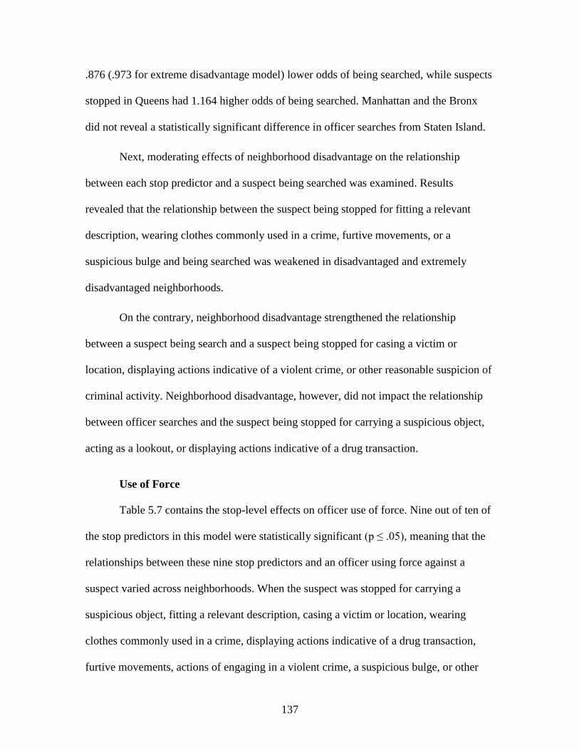
137

.876 (.973 for extreme disadvantage model) lower odds of being searched, while suspects

stopped in Queens had 1.164 higher odds of being searched. Manhattan and the Bronx

did not reveal a statistically significant difference in officer searches from Staten Island.


between each stop predictor and a suspect being searched was examined. Results

revealed that the relationship between the suspect being stopped for fitting a relevant

description, wearing clothes commonly used in a crime, furtive movements, or a

suspicious bulge and being searched was weakened in disadvantaged and extremely

disadvantaged neighborhoods.

On the contrary, neighborhood disadvantage strengthened the relationship

between a suspect being search and a suspect being stopped for casing a victim or

location, displaying actions indicative of a violent crime, or other reasonable suspicion of

criminal activity. Neighborhood disadvantage, however, did not impact the relationship

between officer searches and the suspect being stopped for carrying a suspicious object,

acting as a lookout, or displaying actions indicative of a drug transaction.

Use of Force

Table 5.7 contains the stop-level effects on officer use of force. Nine out of ten of

the stop predictors in this model were statistically significant (p ≤ .05), meaning that the

relationships between these nine stop predictors and an officer using force against a

suspect varied across neighborhoods. When the suspect was stopped for carrying a

suspicious object, fitting a relevant description, casing a victim or location, wearing

clothes commonly used in a crime, displaying actions indicative of a drug transaction,

furtive movements, actions of engaging in a violent crime, a suspicious bulge, or other

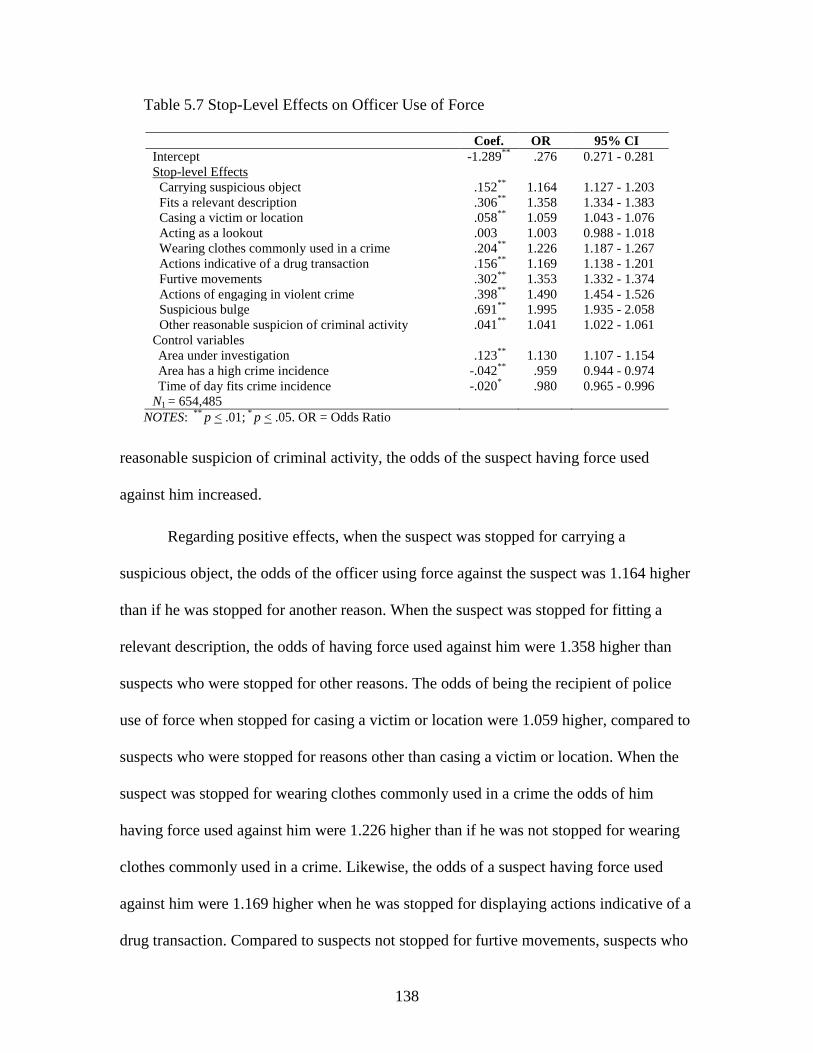
138

Table 5.7 Stop-Level Effects on Officer Use of Force

Coef. OR 95% CI

Intercept -1.289**

.276 0.271 - 0.281

Stop-level Effects


1.164 1.127 - 1.203


1.358 1.334 - 1.383

Casing a victim or location .058**

1.059 1.043 - 1.076

Acting as a lookout .003 1.003 0.988 - 1.018


1.226 1.187 - 1.267


1.169 1.138 - 1.201


1.353 1.332 - 1.374


1.490 1.454 - 1.526


1.995 1.935 - 2.058


1.041 1.022 - 1.061

Control variables


1.130 1.107 - 1.154


.959 0.944 - 0.974

Time of day fits crime incidence -.020* .980 0.965 - 0.996

N1 = 654,485

NOTES: **

p < .01; *


reasonable suspicion of criminal activity, the odds of the suspect having force used

against him increased.


suspicious object, the odds of the officer using force against the suspect was 1.164 higher

than if he was stopped for another reason. When the suspect was stopped for fitting a

relevant description, the odds of having force used against him were 1.358 higher than

suspects who were stopped for other reasons. The odds of being the recipient of police

use of force when stopped for casing a victim or location were 1.059 higher, compared to

suspects who were stopped for reasons other than casing a victim or location. When the

suspect was stopped for wearing clothes commonly used in a crime the odds of him

having force used against him were 1.226 higher than if he was not stopped for wearing

clothes commonly used in a crime. Likewise, the odds of a suspect having force used

against him were 1.169 higher when he was stopped for displaying actions indicative of a

drug transaction. Compared to suspects not stopped for furtive movements, suspects who

139

did display these actions had 1.353 higher odds of having force used against him. When

the suspect was stopped for actions of engaging in a violent crime, the odds of having

force used against him were 1.49 higher than if he was stopped for other reasons.

Compared to suspects not stopped for a suspicious bulge, suspects who did display these

actions had 1.995 higher odds of having force used against him. When the suspect was

stopped for other reasonable suspicion of criminal activity, the odds of being the recipient

of police use of force were 1.041 higher, compared to being stopped for other reasons.

The suspect being stopped for acting as a lookout did not have a statistically

significant effect on officer use of force. In terms of control variables, analyses revealed

that a suspect who was encountered in a neighborhood that is under investigation have

1.130 higher odds of having force used against him. When the suspect was stopped in a

high crime area (.959) or during the time of the day that fit the crime incident (.980) he

has lower odds of being the recipient of police use of force.

Table 5.8 shows the main and moderating effects on officer use of force.24

In both

the concentrated disadvantage and extreme disadvantage models, results revealed that

suspects stopped in neighborhoods with a higher percentage of African-Americans, a

higher percentage of Hispanics, or higher levels of concentrated immigration were more

likely to have force used against them, compared to suspects stopped in neighborhoods

with lower levels of these populations.


most often revealed the same results on all neighborhood-level predictors, except for

disadvantage. There were a few cases where the odds ratios for the predictors differed

between the models. Unless otherwise noted, the differences in neighborhood-level

variables between the models were less than .002.

140

Table 5.8 Main and Moderating Effects on Officer Use of Force




.267 0.263 - 0.272 -1.319**

.267 0.263 - 0.272


1.004 1.004 - 1.005 .004**

1.004 1.003 - 1.005

Percent population Hispanic .005**

1.005 1.004 - 1.006 .004**

1.004 1.003 - 1.005

Percent population recent movers .001 1.001 0.998 - 1.003 .001 1.001 0.999 - 1.004

Percent population renters -.001 .999 0.998 - 1.000 -.001* .999 0.998 - 1.000

Disadvantage -.035* .966 0.935 - 0.998 .011 1.012 0.942 - 1.086


1.104 1.084 - 1.124 .097**

1.102 1.083 - 1.122

Control variables

Manhattan .217**

1.242 1.152 - 1.339 .233**

1.263 1.173 - 1.360

Bronx .293**

1.340 1.238 - 1.452 .275**

1.316 1.215 - 1.426

Brooklyn -.104* .901 0.844 - 0.962 -.095

* .909 0.852 - 0.970

Queens -.044 .957 0.897 - 1.022 -.025 .975 0.916 - 1.039

N2 = 2,114




1.177 1.136 - 1.218 .157**

1.170 1.132 - 1.210

x Disadvantage -.038* .963 0.933 - 0.994 -.093

* .911 0.833 - 0.998


1.378 1.352 - 1.405 .317**

1.373 1.347 - 1.399


.969 0.953 - 0.985 -.108**

.897 0.857 - 0.939

Level-1 Casing a victim or location Effect .074**

1.077 1.059 - 1.094 .070**

1.072 1.055 - 1.089


.970 0.956 - 0.985 -.060* .942 0.899 - 0.987

Level-1 Acting as a lookout Effect .015 1.015 0.999 - 1.031 .012 1.012 0.996 - 1.027

x Disadvantage -.021* .979 0.966 - 0.993 -.025 .976 0.937 - 1.016


1.241 1.199 - 1.285 .217**

1.242 1.201 - 1.284

x Disadvantage -.001 .999 0.971 - 1.028 .011 1.011 0.931 - 1.098


1.211 1.176 - 1.247 .180**

1.197 1.164 - 1.231


.927 0.905 - 0.949 -.187**

.830 0.781 - 0.882


1.371 1.349 - 1.394 .314**

1.369 1.347 - 1.391


.975 0.961 - 0.990 -.070**

.933 0.896 - 0.971


1.484 1.447 - 1.522 .404**

1.498 1.462 - 1.535


1.043 1.020 - 1.067 .075* 1.078 1.010 - 1.151


2.057 1.982 - 2.136 .715**

2.045 1.979 - 2.113


.952 0.925 - 0.980 -.178**

.837 0.783 - 0.894

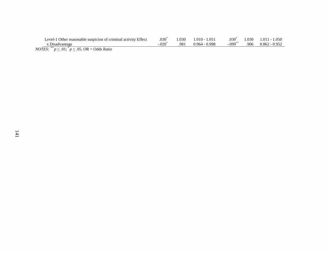
141

Level-1 Other reasonable suspicion of criminal activity Effect .030* 1.030 1.010 - 1.051 .030

* 1.030 1.011 - 1.050

x Disadvantage -.020* .981 0.964 - 0.998 -.099

** .906 0.862 - 0.952

NOTES: **

p < .01; *


142

Regarding positive effects, a suspect stopped in a neighborhood characterized by

a higher percentage of African-Americans had 1.004 higher odds of being the recipient of

force and in a Hispanic neighborhood, the odds were 1.005 higher. When a suspect was

stopped in a neighborhood with higher levels of concentrated immigration, his odds of

having force used against him increased by 1.104 compared to neighborhoods with lower

levels of concentrated immigration. Inverse effects were also apparent. In the

concentrated disadvantage model, a suspect stopped in a more disadvantaged area had

.966 lower odds of having force used against him, while the effect of was not significant

in the extreme disadvantage model. Further, the suspect being stopped in a neighborhood

characterized by higher percentages of recent movers or renters did not impact an

officer’s use of force in either the concentrated disadvantage or extreme disadvantage

models.



1.242 (1.263 for extreme disadvantage model) higher odds of having force used against

him, while suspects stopped in the Bronx had 1.34 (1.316 for extreme disadvantage

model) higher odds of having force used against him. Suspects stopped in Brooklyn had

.901 (.909 in extreme disadvantage model) lower odds of being the recipient of police use

of force, compared to Staten Island. Queens did not reveal a statistically significant

difference in officer use of force from Staten Island.


between each stop predictor and a suspect being the recipient of police use of force was

examined. Results revealed that the relationship between the suspect being stopped for

143

carrying a suspicious object, fitting a relevant description, casing a victim or location,

acting as a lookout,25

displaying actions indicative of a drug transaction, or a suspicious

bulge and being the recipient of police use of force was weakened in disadvantaged and

extremely disadvantaged neighborhoods.


between a suspect being the recipient of police use of force and a suspect being stopped

for displaying actions indicative of a violent crime. Neighborhood disadvantage,

however, did not impact the relationship between police use of force and the suspect

being stopped for wearing clothes commonly used in a crime.

Arrest

Table 5.9 contains the stop-level effects on officer arrests. Eight out of ten of the

Table 5.9 Stop-Level Effects on Officer Arrests

Coef. OR 95% CI

Intercept -1.873**

.154 (0.152,0.155)

Stop-level Effects


1.755 (1.699,1.813)


1.465 (1.442,1.488)


.973 (0.963,0.982)

Acting as a lookout .008 1.008 (0.999,1.017)


1.126 (1.106,1.147)


1.693 (1.647,1.740)

Furtive movements -.002 .998 (0.989,1.006)


1.157 (1.141,1.173)


1.142 (1.123,1.160)


1.269 (1.251,1.287)

Control variables


1.063 (1.050,1.076)


.933 (0.925,0.941)

Time of day fits crime incidence .012* 1.012 (1.003,1.020)

N1 = 654,485

NOTES: **

p < .01; *


25 The relationship between the suspect acting as a lookout and being the recipient of

police use of force was not moderated by extreme disadvantage.

144

stop predictors in this model were statistically significant (p ≤ .05), meaning that the

relationships between these eight stop predictors and an officer arresting a suspect varied

across neighborhoods. When the suspect was stopped for carrying a suspicious object,

fitting a relevant description, wearing clothes commonly used in a crime, displaying

actions indicative of a drug transaction, displaying actions of engaging in a violent crime,

a suspicious bulge, or other reasonable suspicion of criminal activity, the odds of the

suspect being arrested increased.


suspicious object, the odds of being arrested were 1.755 higher than suspects who were

stopped for other reasons. The odds of being arrested when the suspect was stopped for

fitting a relevant description were 1.465 higher, compared to suspects who were stopped

for reasons other than fitting a relevant description. When the suspect was stopped for

wearing clothes commonly used in a crime the odds of him being arrested were 1.126

higher than if he was not stopped for wearing clothes commonly used in a crime.

Likewise, the odds of a suspect being arrested were 1.693 higher when he was stopped

for displaying actions indicative of a drug transaction. When the suspect was stopped for

actions of engaging in a violent crime, the odds of being arrested were 1.157 higher than

if he was stopped for not displaying these actions. Similarly, when the suspect was

stopped for a suspicious bulge, the odds of being arrested were 1.142 higher, compared to

being stopped for other reasons. And, the odds of a suspect being arrested were 1.269

higher when he was stopped for other reasonable suspicion of criminal activity.

Conversely, inverse effects showed that when the suspect was stopped for casing

a victim or location, his odds of being arrested were .973 lower, compared to being

145

stopped for reasons other than casing a victim or location. The suspect being stopped for

acting as a lookout and furtive movements did not have a statistically significant effect on

officer arrests.


encountered in a neighborhood that is under investigation (OR = 1.063) or during the

time of the day that fit the crime incident (OR = 1.012) had higher odds of being arrested.

However, when the suspect was stopped in a high crime neighborhood, the odds of being

arrested were .993 lower, compared to suspects stopped in low crime neighborhoods.

Table 5.10 shows the main and moderating effects on officer arrests. In both the


suspects stopped in a neighborhood with a higher percentage of African-Americans or a

higher percentage of Hispanics were less likely to be arrested, compared to suspects

stopped in a neighborhood with lower levels of these populations. A suspect stopped in a

neighborhood characterized by a higher percentage of African-Americans had .999 lower

odds of being arrested and suspect stopped in a neighborhood with a higher percentage of

Hispanics had .998 lower odds of being arrested. A suspect stopped in neighborhoods

with higher percentages of recent movers, renters, or higher levels of concentrated

immigration did not significantly impact an officer’s decision to arrest.

In the concentrated disadvantage model, disadvantage was a statistically

significant predictor of officer arrests; suspects stopped in disadvantaged neighborhoods

had 1.030 higher odds of being arrested, compared to suspects stopped in more affluent

areas. Extreme disadvantage, however, was not a statistically significant predictor of

officer arrests; differences in an officer’s decision to arrest a suspect in an extremely

146

Table 5.10 Main and Moderating Effects on Officer Arrests




.147 0.146 - 0.148 -1.918**

.147 0.146 - 0.148


.999 0.998 - 0.999 -.001**

.999 0.999 - 0.999


.998 0.997 - 0.999 -.002**

.998 0.998 - 0.999

Percent population recent movers -.001 .999 0.998 - 1.001 -.001 .999 0.998 - 1.001

Percent population renters .0041 1.000 0.999 - 1.000 .001

1 1.000 0.999 - 1.000

Disadvantage .029* 1.030 1.010 - 1.051 .018 1.018 0.979 - 1.058

Concentrated immigration -.009

.991 0.979 - 1.002 -.008

.993 0.981 - 1.004

Control variables

Manhattan .207**

1.230 1.164 - 1.299 .193**

1.213 1.149 - 1.281

Bronx .076* 1.079 1.024 - 1.137 .083

* 1.087 1.031 - 1.146

Brooklyn -.012 .988 0.943 - 1.034 -.019 .981 0.938 - 1.027

Queens .171**

1.187 1.133 - 1.244 .157**

1.169 1.117 - 1.224

N2 = 2,114




1.841 1.780 - 1.905 .610**

1.841 1.781 - 1.902

x Disadvantage .029 1.029 0.997 - 1.062 .133* 1.142 1.040 - 1.253


1.533 1.508 - 1.558 .424**

1.528 1.504 - 1.553


.940 0.928 - 0.953 -.159**

.853 0.821 - 0.887


.951 0.941 - 0.962 -.049**

.952 0.942 - 0.962

x Disadvantage -.004 .996 0.986 - 1.005 .011 1.011 0.984 - 1.038


1.044 1.033 - 1.054 .042**

1.043 1.033 - 1.053


.973 0.965 - 0.982 -.053**

.948 0.924 - 0.973


1.172 1.148 - 1.197 .159**

1.173 1.150 - 1.196

x Disadvantage -.018* .982 0.967 - 0.997 -.055

* .946 0.912 - 0.982


1.806 1.753 - 1.861 .590**

1.805 1.755 - 1.856

x Disadvantage .009 1.009 0.985 - 1.033 .020 1.020 0.957 - 1.088


.982 0.973 - 0.991 -.019**

.981 0.973 - 0.990


.968 0.959 - 0.976 -.070**

.933 0.911 - 0.955


1.194 1.176 - 1.213 .177**

1.194 1.177 - 1.211


.970 0.958 - 0.983 -.068**

.934 0.904 - 0.965


1.167 1.142 - 1.193 .141**

1.151 1.130 - 1.173


.919 0.906 - 0.933 -.178**

.837 0.811 - 0.863

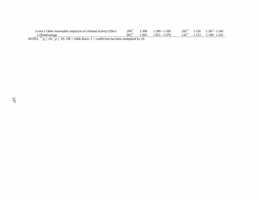
147


1.308 1.289 - 1.328 .282**

1.326 1.307 - 1.345


1.065 1.051 - 1.079 .143**

1.153 1.108 - 1.201

NOTES: **

p < .01; *

p < .05. OR = Odds Ratio; 1 = coefficient has been multiplied by 10.

148

disadvantaged neighborhood and a less disadvantaged neighborhood were not apparent.

Results for control variables at the neighborhood-level revealed similarities between the

two models. Compared to Staten Island, a suspect stopped in Manhattan had 1.23 (1.213

for extreme disadvantage model) higher odds of being arrested. Likewise, suspects

stopped in the Bronx had 1.079 higher odds of being arrested and suspects stopped in

Queens had 1.187 (1.169 for extreme disadvantage model) higher odds of being arrested,

compared to suspects stopped in Staten Island. Brooklyn did not reveal a statistically

significant difference in officer arrests from Staten Island.


between each stop predictor and a suspect being arrested was examined. Results revealed

that the relationship between the suspect being stopped for fitting a relevant description,

acting as a lookout, wearing clothes commonly used in a crime, furtive movements,

displaying action indicative of a violent crime, or a suspicious bulge and being arrested

was weakened in disadvantaged and extremely disadvantaged neighborhoods.


between a suspect being arrested and a suspect being stopped for other reasonable

suspicion of criminal activity. Also, extreme disadvantage strengthened the relationship

between a suspect being arrested and a suspect being stopped for carrying a suspicious

object. Concentrated disadvantage did not moderate the relationship between a suspect

being arrested and a suspect being stopped for carrying a suspicious object, while neither

concentrated disadvantage or extreme disadvantage moderated the relationship between a

suspect being arrested and the suspect being stopped for casing a victim or location, or

being stopped for displaying actions indicative of a drug transaction.

149

5.2 Coercive Action Continuum

Table 5.11 contains the stop-level effects on the coercive action continuum. All of

Table 5.11 Stop-Level Effects on Coercive Action Continuum

Coef. (SE)

Intercept 3.040**

(.01)

Stop-level Effects (.05)

Carrying suspicious object 1.186**

(.02)

Fits a relevant description 1.022**

(.01)


(.01)

Acting as a lookout -.156**

(.03)


(.04)

Actions indicative of a drug transaction 1.017**

(.01)


(.02)


(.03)

Suspicious bulge 1.379**

(.02)


(.01)

Control variables


(.02)


(.01)


(.01)

N1 = 654,485

NOTES: **

p < .01; *

p < .05

the stop predictors in this model were statistically significant (p ≤ .05), meaning that the

relationships between the stop predictors and an officer’s decision to use coercion varied

across neighborhoods. When the suspect was stopped for carrying a suspicious object,

fitting a relevant description, wearing clothes commonly used in a crime, displaying

actions indicative of a drug transaction, furtive movements, displaying actions of

engaging in a violent crime, a suspicious bulge, or other reasonable suspicion of criminal

activity, his likelihood of receiving higher levels of coercive action increased.

Regarding positive effects, the suspect being stopped for carrying a suspicious

object was associated with a 1.19 unit increase in the coercive action used against him.

The coercive action used against a suspect when stopped for fitting a relevant description

increased by 1.02 units. When the suspect was stopped for wearing clothes commonly

150

used in a crime, he was .28 units higher on the coercive action continuum. Likewise, the

suspect being stopped for displaying actions indicative of a drug transaction was

associated with a 1.02 unit increase in the coercive action used against him. The coercive

action used against a suspect when stopped for furtive movements increased by .53 units.

When the suspect was stopped for displaying actions indicative of violent crime, he was

.64 units higher on the coercive action continuum. The suspect being stopped for a

suspicious bulge was associated with a 1.38 unit increase in the coercive action used

against him. And, when the suspect was stopped for other reasonable suspicion of

criminal activity, he was .33 units higher on the coercive action continuum.

Conversely, inverse effects showed that being stopped for casing a victim or

location or acting as a lookout was associated with a decrease in the amount of coercive

action he received. When the suspect was stopped for casing a victim or location, he was

.12 units lower on the coercive action continuum. Lastly, when the suspect was stopped

for acting as a lookout, he was .16 units lower on the coercive action continuum.


encountered in a neighborhood that is under investigation has a higher likelihood of

receiving greater coercive action (.19 unit increase). However, the suspect being stopped

in a high crime neighborhood (-.23) or during the time of the day that fit the crime

incident (-.059) was associated with a reduction in the coercive action used against him.

Table 5.12 shows the main and moderating effects on the coercive action

continuum. In both the concentrated disadvantage and extreme disadvantage models,

results revealed a positive association between suspects being stopped in a neighborhood

with a higher percentage of African-Americans, a higher percentage of Hispanics, or

151

Table 5.12 Main and Moderating Effects on Coercive Action Continuum


Coef. (SE) Coef. (SE)

Stop-level Main Effects (intercept as outcome) 3.021**

(.01) 3.021**

(.01)


(.001) .002**

(.0004)

Percent population Hispanic .002* (.001) .002

* (.0006)

Percent population recent movers -.002 (.002) -.003 (.002)

Percent population renters .001 (.001) .001 (.0007)

Disadvantage .036 (.02) .181**

(.05)


(.01) .102**

(.01)

Control variables

Manhattan .328**

(.06) .331**

(.06)

Bronx .332**

(.06) .302**

(.06)

Brooklyn -.194**

(.05) -.191**

(.05)

Queens .236**

(.05) .226**

(.05)

N2 = 2,114



Level-1 Carrying suspicious object Effect 1.197**

(.05) 1.193**

(.05)

x Disadvantage .004 (.05) .206 (.14)

Level-1 Fits a relevant description Effect 1.058**

(.02) 1.044**

(.02)


(.02) -.398**

(.05)


(.01) -.113**

(.01)


(.01) -.095* (.04)

Level-1 Acting as a lookout Effect -.139**

(.01) -.151**

(.01)


(.01) -.078* (.03)


(.03) .290**

(.03)

x Disadvantage -.073* (.02) -.165

* (.06)

Level-1 Actions indicative of a drug transaction Effect 1.053**

(.04) 1.037**

(.04)


(.04) -.313**

(.08)


(.01) .533**

(.01)


(.01) -.156**

(.03)


(.02) .642**

(.02)

x Disadvantage -.016 (.02) -.020 (.05)

Level-1 Suspicious bulge Effect 1.482**

(.04) 1.420**

(.03)


(.03) -.553**

(.05)

152


(.02) .332**

(.02)

x Disadvantage .053* (.02) .078 (.06)

NOTES: **

p < .01; *

p < .05

153

higher levels of concentrated immigration and greater coercive action. For every one

percent increase in African-American population or Hispanic population, the suspect’s

likelihood of receiving greater levels of coercive action increases by .002 units. Similarly,

for every one unit increase in concentrated immigration, the suspect’s likelihood of

receiving greater levels of coercive action increases by .10 units. In both models, a

suspect stopped in neighborhoods with higher percentages of recent movers or renters did

not significantly impact an officer’s decision to use coercion.

In the concentrated disadvantage model, disadvantage was not a statistically

significant predictor of officer use of coercion. However, suspects who were encountered

in extremely disadvantage neighborhoods had a higher likelihood of receiving greater

levels of coercive action (.18 unit increase). Results for control variables at the

neighborhood-level revealed similarities between the two models. Compared to Staten

Island, a suspect stopped in Manhattan was associated with a .33 unit increase in the

coercive action continuum; suspects stopped in the Bronx increased the level of coercion

by .33 units (.30 for extreme disadvantage model); and suspects stopped in Queens

increased the level of coercion by .23 units. Suspects encountered in Brooklyn, however,

were associated with a .19 unit decrease in the coercive action continuum. Compared to

Staten Island, officers in Brooklyn use less serious forms of coercive action when

stopping a suspect.


between each stop predictor and the coercive action continuum was examined. Results

revealed that the relationship between the suspect being stopped for fitting a relevant

description, casing a victim or location, acting as a lookout, wearing clothes commonly

154

used in a crime, displaying actions indicative of a drug transaction, furtive movements, or

a suspicious bulge and receiving greater levels of coercive action was weakened in

disadvantaged and extremely disadvantaged neighborhoods.

On the contrary, concentrated disadvantage strengthened the relationship between

a suspect receiving greater levels of coercive action and a suspect being stopped for other

reasonable suspicion of criminal activity. Neighborhood disadvantage did not moderate

the relationship between a suspect receiving greater levels of coercive action and the

suspect being stopped for carrying a suspicious object or displaying actions indicative of

a violent crime. Further, extreme disadvantage did not moderate the relationship between

a suspect receiving greater levels of coercive action and the suspect being stopped for

other reasonable suspicion of criminal activity.

5.3 Highest Level of Coercive Action Used

Table 5.13 contains the stop-level effects on the highest level of coercion used

outcome. Nine out of ten of the stop predictors in this model were statistically significant

(p ≤ .05), meaning that the relationships between these nine stop predictors and an

officer’s level of coercion varied across neighborhoods. When the suspect was stopped

for carrying a suspicious object, fitting a relevant description, wearing clothes commonly

used in a crime, displaying actions indicative of a drug transaction, furtive movements,

displaying actions of engaging in a violent crime, or a suspicious bulge, the odds of the

suspect being in a higher category of coercive action used against him decreased.

When the suspect was stopped for carrying a suspicious object, the odds of being

in a higher category of coercion were .641 lower than suspects who were stopped for

other reasons. The odds of being in a higher category of coercion when the suspect was

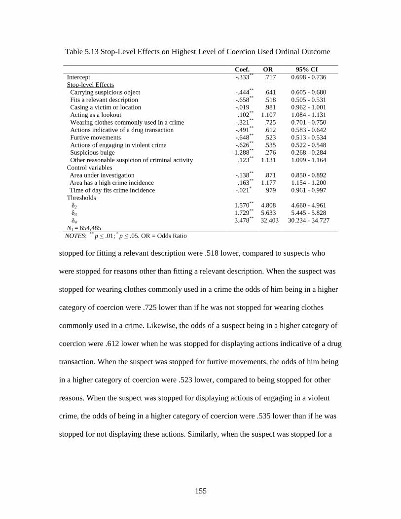
155

Table 5.13 Stop-Level Effects on Highest Level of Coercion Used Ordinal Outcome

Coef. OR 95% CI

Intercept -.333**

.717 0.698 - 0.736

Stop-level Effects

Carrying suspicious object -.444**

.641 0.605 - 0.680

Fits a relevant description -.658**

.518 0.505 - 0.531

Casing a victim or location -.019 .981 0.962 - 1.001

Acting as a lookout .102**

1.107 1.084 - 1.131

Wearing clothes commonly used in a crime -.321**

.725 0.701 - 0.750

Actions indicative of a drug transaction -.491**

.612 0.583 - 0.642

Furtive movements -.648**

.523 0.513 - 0.534

Actions of engaging in violent crime -.626**

.535 0.522 - 0.548

Suspicious bulge -1.288**

.276 0.268 - 0.284


1.131 1.099 - 1.164

Control variables

Area under investigation -.138**

.871 0.850 - 0.892

Area has a high crime incidence .163**

1.177 1.154 - 1.200

Time of day fits crime incidence -.021* .979 0.961 - 0.997

Thresholds

δ2 1.570**

4.808 4.660 - 4.961

δ3 1.729**

5.633 5.445 - 5.828

δ4 3.478**

32.403 30.234 - 34.727

N1 = 654,485

NOTES: **

p < .01; *


stopped for fitting a relevant description were .518 lower, compared to suspects who

were stopped for reasons other than fitting a relevant description. When the suspect was

stopped for wearing clothes commonly used in a crime the odds of him being in a higher

category of coercion were .725 lower than if he was not stopped for wearing clothes

commonly used in a crime. Likewise, the odds of a suspect being in a higher category of

coercion were .612 lower when he was stopped for displaying actions indicative of a drug

transaction. When the suspect was stopped for furtive movements, the odds of him being

in a higher category of coercion were .523 lower, compared to being stopped for other

reasons. When the suspect was stopped for displaying actions of engaging in a violent

crime, the odds of being in a higher category of coercion were .535 lower than if he was

stopped for not displaying these actions. Similarly, when the suspect was stopped for a

156

suspicious bulge, the odds of being in a higher category of coercion were .276 lower,

compared to being stopped for other reasons.

Conversely, when the suspect was stopped for acting as a lookout, his odds of

being in a higher category of coercion were 1.107 higher, compared to being stopped for

reasons other than acting as a lookout. And, the odds of a suspect being in a higher

category of coercion were 1.131 higher when he was stopped for other reasonable

suspicion of criminal activity. The suspect being stopped for casing a victim or location

did not have a statistically significant effect on the ordinal outcome. In terms of control

variables, analyses revealed that a suspect who was encountered in a neighborhood that is

under investigation (OR = .871) or during the time of the day that fit the crime incident

(OR = .979) had lower odds of being in a higher category of coercion. However, when

the suspect was stopped in a high crime neighborhood, the odds of being in a higher

category of coercion were 1.177 higher, compared to suspects stopped in low crime

neighborhoods.

Table 5.14 shows the main and moderating effects on the highest level of coercion

used outcome. 26

In both the concentrated disadvantage and extreme disadvantage

models, results revealed that suspects stopped in a neighborhood with a higher percentage

of African-Americans, a higher percentage of Hispanics, or higher levels of concentrated

immigration were less likely to be in a higher category of coercion, compared to suspects


most often revealed the same results on all neighborhood-level predictors. There were a

few cases where the odds ratios for the predictors differed between the models. Unless

otherwise noted, the differences in neighborhood-level variables between the models

were less than .001.

157

Table 5.14 Main and Moderating Effects on Highest Level of Coercion Used Ordinal Outcome



Stop-level Main Effects (intercept as outcome) -.317**

.728 .712 - 0.745 -.317**

.728 0.712 - 0.745


.996 .995 - 0.997 -.004**

.996 0.996 - 0.997


.996 .995 - 0.997 -.003**

.997 0.996 - 0.998

Percent population recent movers .002 1.002 .999 - 1.005 .002 1.002 0.999 - 1.004

Percent population renters -.001 .999 .998 - 1.000 .0031

1.000 0.999 - 1.001

Disadvantage .027 1.028 .994 - 1.062 .026 1.026 0.962 - 1.094

Concentrated immigration -.109**

.897 .877 - 0.917 -.107**

.898 0.879 - 0.919

Control variables

Manhattan -.179**

.836 .757 - 0.924 -.189**

.827 0.750 - 0.913

Bronx -.276**

.759 .688 - 0.836 -.272**

.762 0.691 - 0.840

Brooklyn .148**

1.159 1.061 - 1.266 .142* 1.152 1.056 - 1.258

Queens -.203**

.816 .748 - 0.892 -.216**

.805 0.739 - 0.878

N2 = 2,114



Level-1 Carrying suspicious object Effect -.458**

.633 0.595 - 0.673 -.447**

.640 0.603 - 0.679

x Disadvantage .067* 1.069 1.012 - 1.131 .031 1.031 0.884 - 1.203

Level-1 Fits a relevant description Effect -.672**

.510 0.497 - 0.524 -.663**

.516 0.502 - 0.529


1.086 1.061 - 1.111 .222**

1.248 1.169 - 1.333

Level-1 Casing a victim or location Effect -.033* .967 0.947 - 0.988 -.022

* .978 0.958 - 0.998


1.079 1.060 - 1.098 .140**

1.151 1.095 - 1.209


1.091 1.067 - 1.115 .097**

1.101 1.078 - 1.125


1.070 1.050 - 1.091 .103**

1.108 1.051 - 1.169

Level-1 Wearing clothes commonly used in a crime Effect -.321**

.725 0.697 - 0.755 -.323**

.724 0.699 - 0.751

x Disadvantage .026 1.026 0.996 - 1.057 .083* 1.087 1.009 - 1.170

Level-1 Actions indicative of a drug transaction Effect -.519**

.595 0.565 - 0.627 -.500**

.607 0.577 - 0.638


1.162 1.114 - 1.213 .339**

1.403 1.271 - 1.549


.522 0.511 - 0.533 -.646**

.524 0.513 - 0.535


1.047 1.029 - 1.065 .134**

1.143 1.090 - 1.199

Level-1 Actions of engaging in violent crime Effect -.622**

.537 0.522 - 0.552 -.618**

.539 0.525 - 0.553

x Disadvantage .030* 1.031 1.008 - 1.054 .086

* 1.090 1.026 - 1.157

Level-1 Suspicious bulge Effect -1.321**

.267 0.257 - 0.277 -1.277**

.279 0.270 - 0.288

x Disadvantage .172* 1.188 1.155 - 1.221 .397

** 1.488 1.399 - 1.582

158


1.125 1.092 - 1.160 .120**

1.128 1.096 - 1.160

x Disadvantage .007 1.007 0.982 - 1.033 .035 1.035 0.959 - 1.117

NOTES: **

p < .01; *

p < .05; 1 = coefficient has been multiplied by 10.

159

stopped in a neighborhood with lower levels of these populations. A suspect stopped in a

neighborhood characterized by a higher percentage of African-Americans and a higher

percentage of Hispanics had .996 lower odds of being in a higher category of coercion.

The odds of a suspect being in a higher category of coercion were .897 lower when

stopped in neighborhoods marked by higher levels of concentrated immigration. A

suspect stopped in neighborhoods with higher percentages of recent movers, renters, or

higher levels of disadvantage did not significantly impact an officer’s decision to use

coercion.



.836 (.827 for extreme disadvantage model) lower odds of being in a higher category of

coercion. Likewise, suspects stopped in the Bronx had .759 (.762 for extreme

disadvantage model) lower odds of being in a higher category of coercion and suspects

stopped in Queens had .816 (.805 for extreme disadvantage model) lower odds of being

arrested, compared to suspects stopped in Staten Island. On the other hand, suspects

stopped in Brooklyn faced a 1.159 (1.152 for extreme disadvantage model) higher odds

of being in a higher category of coercion, compared to Staten Island.


between each stop predictor and the highest level of coercion used was examined. Results

revealed that the relationship between the suspect being in a higher category of coercive

action and being stopped for any of the stop predictors listed in the UF-250 report was

strengthened by neighborhood disadvantage. There were a few exceptions: concentrated

disadvantage did not moderate the relationship between a suspect being in a higher

160

category of coercive action and being stopped for wearing clothes commonly used in a

crime or a suspicious bulge, while extreme disadvantage did not moderate the

relationship between a suspect being in a higher category of coercive action and being

stopped for carrying a suspicious object or other reasonable suspicion of criminal

activity.

161

CHAPTER 6

DISCUSSION AND CONCLUSION

6.1 Discussion of Results

Researchers have observed that community characteristics are thought to be more

statistically consistent in explaining an officer’s decision to act coercively, compared to

the other conceptual frameworks (situational factors, officer characteristics, and

organizational factors) (National Research Council, 2004). Although researchers have

uncovered an important link between the structural features of the community and an

officer’s decision-making behavior (e.g., Kane, 2002; Sun et al., 2008), the role of

neighborhood social disorganization applied to police decision-making during street

encounters has been understudied. This study attempts to fill this gap by examining the

influence of concentrated disadvantage (and extreme disadvantage) on the relationship

between the reason for the stop (e.g., suspect fits a relevant description) and an officer’s

use of coercion that may occur during a PCI (e.g., frisk, search, use of force, or arrest).

Two main hypotheses were tested in this study: (1) how the factors of neighborhood

disorganization effect an officer’s decision to use coercion (main effects) and (2) how

neighborhood disadvantage impacts (or moderates) the relationship between the stop

predictors and the coercive action the officer uses during the stop. The analyses revealed

several patterns, which are discussed below.

162

Summary of Main Effects

In order to examine the effects of social disorganization on police use of coercion,

the contemporary disorganization measures were used in this analysis. Table 6.1 depicts

the summary of the main effects of the social disorganization measures on police use of

coercion. One notable finding is that there are apparent similarities in communities

marked by a higher percentage of African-Americans, a higher percentage of Hispanics,

and a higher rate of concentrated immigration. Generally speaking, suspects stopped in

communities with higher levels of these populations were more likely to be frisked, to be

the recipient of police use of force, and to be on the more coercive end of the coercive

action continuum. They were, however, less likely to be searched, arrested, and to be in a

higher category of coercive action.27

Although this study did not specifically analyze the individual-level effect of the

suspect’s race on police use of coercion, it can be seen that police are more active in

communities characterized by higher amounts of minority populations. These results

seem to provide support for arguments that police may be threatened by increases in

minority populations. Some researchers would argue that the components of conflict

theory, racial discrimination, racial profiling, institutional racism, and racial threat are

apparent in the NYPD, where officers impose increased social controls on minorities in

order to keep them powerless (see e.g., Eitle, 2002; Link and Phelan, 2001; Trone, 2010;

Walker et al., 2000). Findings from this study are consistent with the findings from past

27 Concentrated immigration was not a statistically significant predictor of officer

searches or arrests

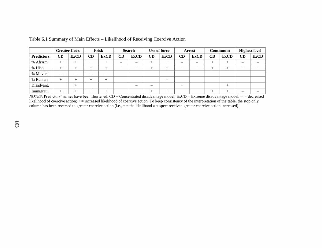
163

Table 6.1 Summary of Main Effects – Likelihood of Receiving Coercive Action

Greater Coer. Frisk Search Use of force Arrest Continuum Highest level

Predictors CD ExCD CD ExCD CD ExCD CD ExCD CD ExCD CD ExCD CD ExCD

% AfrAm. + + + + – – + + – – + + – –

% Hisp. + + + + – – + + – – + + – –

% Movers – – – –

% Renters + + + + –

Disadvant. + – – + +

Immigrat. + + + + + + + + – –

NOTES: Predictors’ names have been shortened. CD = Concentrated disadvantage model; ExCD = Extreme disadvantage model. – = decreased

likelihood of coercive action; + = increased likelihood of coercive action. To keep consistency of the interpretation of the table, the stop only

column has been reversed to greater coercive action (i.e., + = the likelihood a suspect received greater coercive action increased).

164

studies examining racial discrimination within the NYPD, stating that minorities are

stopped and frisked at a much higher rate than whites, while controlling for other factors

(Fagan, 2012; Gelman et al., 2007); findings also contradict Lee et al.’s conclusions

(2010) that police use of force is not related to the community’s percent of minority

population.

Although suspects stopped in neighborhoods characterized by higher levels of

minorities are more likely to be frisked and be the recipients of police use of force, they

face lower odds of being searched and arrested. Officers may be more willing to frisk and

use force against suspects encountered in these communities, potentially because the laws

outlining these actions are less explicit than search and arrest, where the law states a

specific need for probable cause. It seems that there may be a point where the law steps in

to prevent outright discrimination and avert further punitive action against minorities,

what several court rulings (e.g., Terry v. Ohio; Tennessee v. Garner) were designed to

accomplish.

Contrary to the view that NYPD officers are discriminatory toward suspects

encountered in areas with higher levels of minorities, some researchers would argue that

police are choosing their targets based on patterns of criminal activity and the “typical”

offender (Smith et al., 2006). For example, Fagan and Davies (2000) explained that racial

profiling is often based on the officer’s prior knowledge and reasonable suspicion;

therefore, some would argue that results for this study may be explained by officers

simply doing their job based on their past experiences and knowledge of crime patterns.

Turning our attention to the residential instability component of social

disorganization, recall that scholars often use the community’s percentage of recent

165

movers and the percentage of renters in an index that represents the unstable environment

that may be associated with higher levels of criminal activity (Sampson et al., 1997).

These two variables were included separately in this analysis because they did not load

on the same factor; analyses of these variables revealed contradictory findings. Suspects

stopped in neighborhoods marked by a higher percentage of recent movers were less

likely to be stopped and frisked, while suspects stopped in neighborhoods marked by a

higher percentage of renters were more likely to be stopped and frisked. It may be that in

New York City, moving residences is more commonplace and officers do not see this as

an indicator or predictor of problem behaviors or criminal activity, while lower rates of

home ownership remains a predictor of problem behaviors (see Brooks-Gunn et al.,

1993).

The main focus of this study, neighborhood disadvantage, was used to represent a

community’s social and economic indicators (see Land et al., 1990). Results revealed that

neighborhood disadvantage (and extreme disadvantage) was not a statistically significant

predictor of police coercive action in many instances. Although, results did reveal that

suspects encountered in disadvantaged areas were less likely to have force used against

them and more likely to be arrested, while suspects encountered in extremely

disadvantaged areas were less likely to be searched and more likely to be on the higher

end of the coercive action continuum. In hindsight it does not seem that neighborhood

disadvantage plays a substantial role in predicting an officer’s use of coercive action;

however, moderating effects tell a different story.

166

Summary of Moderating Effects

Table 6.2 provides a summary of the effects of concentrated disadvantage and

extreme disadvantage on the relationship between each stop predictor and each outcome.

Concentrated disadvantage and extreme disadvantage had the same directional impact

(e.g., strengthening or weakening) on the relationship between each stop predictor and

each outcome. There were a few instances when one of the models had a statistically

significant impact (e.g., concentrated disadvantage), yet the other model did not (e.g.,

extreme disadvantage). Regardless, a few overall patterns emerged.

The general pattern of the moderating effects is that neighborhood disadvantage

weakens the positive relationship between the stop predictors and coercive action. In

other words, a suspect who is stopped for at least one of the reasons listed on the UF-250

report in a disadvantaged (or extremely disadvantaged) neighborhood faces a lower

likelihood of having coercive action used against him. This is a key finding for this study.

Although neighborhood disadvantage did not have a substantial main effect on an

officer’s use of coercive action, the moderating effects show support for the alternative

hypothesis that officers who work in disadvantaged areas may be less likely to act

coercively during a PCI.

This study reasoned three theoretical connections between a community’s level of

social disorganization, normally predicting crime within a community, and an officer’s

decision-making. The first and second theoretical connections argued that police would

become more coercive in disorganized and disadvantaged neighborhoods as a result of

the high amount of crime and lack of formal social controls observed in these areas (e.g.,

Terrill and Reisig, 2003). The third theoretical connection posited that police would

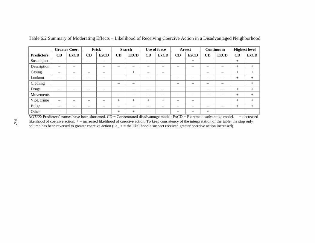
167

Table 6.2 Summary of Moderating Effects – Likelihood of Receiving Coercive Action in a Disadvantaged Neighborhood

Greater Coer. Frisk Search Use of force Arrest Continuum Highest level

Predictors CD ExCD CD ExCD CD ExCD CD ExCD CD ExCD CD ExCD CD ExCD

Sus. object – – – – – – + +

Description – – – – – – – – – – – + +

Casing – – – – + – – – – + +

Lookout – – – – – – – – – + +

Clothing – – – – – – +

Drugs – – – – – – – – – + +

Movements – – – – – – – – + +

Viol. crime – – – – + + + + – – + +

Bulge – – – – – – – – – – – – + +

Other – – – – + + – – + + +

NOTES: Predictors’ names have been shortened. CD = Concentrated disadvantage model; ExCD = Extreme disadvantage model. – = decreased

likelihood of coercive action; + = increased likelihood of coercive action. To keep consistency of the interpretation of the table, the stop only

column has been reversed to greater coercive action (i.e., + = the likelihood a suspect received greater coercive action increased).

168

become less coercive in these areas because they are overworked and these areas are

more accepting of deviant behaviors (e.g., Klinger, 1997).

Overall, findings from this study support the third theoretical connection that

police are less likely to use coercive action against suspects encountered in disadvantaged

areas. Main effects of disadvantage on coercive action provided mixed and, often times,

statistically insignificant results. However, results from moderating effects provide

support for Khruakham and Hoover’s (2012) findings that officers use less coercion in

disadvantaged neighborhoods. The general pattern is that neighborhood disadvantage acts

as a weakening mechanism on the relationship between each stop predictor and the

coercive action used during the stop. When a suspect is stopped, his chances of receiving

any level of coercive action are reduced, if the stop occurred in a disadvantaged

neighborhood.

As a result of the sheer number of stops made in disadvantaged neighborhoods,

suspects potentially face lower odds of receiving coercive action. A person may be more

likely to be subjected to a stop in a disadvantaged and high crime neighborhood, but the

odds of having coercion used against him is lower than if stopped in an affluent

neighborhood. For example, if 100 stops were made in a disadvantaged neighborhood a

suspect may have a 1/10 chance of having coercive action used against him; if 10 stops

were made in an affluent neighborhood, the suspect may face a 1/3 chance of having

coercive action used against him. Results from this study should not be interpreted as

coercive action occurring less frequently in disadvantaged neighborhoods per se, only

that disadvantage has a reduction effect on the coercive action an officer uses in each

stop. It very well may be that higher levels of coercive action occur more frequently in

169

disadvantaged neighborhoods, yet a suspect faces a lower likelihood of receiving greater

levels of coercive action in disadvantaged neighborhoods.

Results from this study also lend support to Klinger’s (1997) ecological theory of

police behavior. Klinger (1997) argued that residents perceive deviance as more

accepting in disadvantaged communities and that officers are too busy with heavy

workloads, which may cause officers to handle only the most serious offenses formally.

This could be the case for NYPD stops made in 2011, which explains why neighborhood

disadvantage reduces the chances of a suspect receiving greater levels of coercive action

when stopped. When low-level criminal behavior (e.g., simple drug possession) is

tolerated in disadvantage communities and occurs frequently, suspects face a lower risk

of receiving higher levels of coercive action. Further, because police resources are slim

and low-level criminal behavior is tolerated in these areas, a suspect stopped in a

disadvantaged neighborhood has a lower likelihood of having coercive action used

against him. If this same scenario played out in an affluent neighborhood, where police

resources are abundant enough to apply coercion to low-level crimes, a suspect stopped

would face a higher likelihood of having coercive action used against him.

There are, however, a few exceptions to the general pattern found in the data

analyses. Extreme disadvantage increases the likelihood a suspect will be searched when

he is stopped for casing a victim or location. And, extreme disadvantage increases the

likelihood a suspect will be arrested when he is stopped for carrying a suspicious object.

Further, the stop predictors displaying actions indicative of a violent crime and other

reasonable suspicion of criminal activity often behave dissimilar to the general pattern.

170

When a suspect is stopped for displaying actions indicative of a violent crime, he

is more likely to be subjected to a search or police use of force when stopped in a

disadvantaged neighborhood. It may be that when an officer believes a suspect is

involved in committing a violent offense, the officer’s feelings to protect himself

increases because of his perception of harm (Brown, 1981). The perception of harm

would then lead to a greater likelihood of the suspect experiencing a search or police use

of force.

In terms of the suspect being stopped for other reasonable suspicion of criminal

activity in a disadvantaged neighborhood, he is more likely to be searched, arrested, and

to receive higher levels of coercive action (as determined by the coercive action

continuum). Suspects stopped for other reasonable suspicion of criminal activity may

encompass a wide variety of potential criminal conduct not outlined in the UF-250 report,

making it difficult to speculate as to why this relationship occurs. Further, it may be that

individual-level factors not included in this analysis are having an impact on this

relationship. For example, scholars have reasoned that the amount of coercive action used

by police may be attributed to the behavior of the suspect (Sun and Payne, 2004; Sun et

al., 2008). These individual-level factors, however, are not included in this study, but

may potentially help explain some of the dissimilar relationships to the general pattern.

Another noteworthy finding is that the highest level of coercion used outcome

provides results contrary to the general pattern. For this outcome, the relationship

between each stop predictor and a suspect being in a higher category of coercive action is

strengthened by neighborhood disadvantage. This could potentially be explained by the

differences in measures between the two outcomes. Recall that the coercive action

171

continuum considered all possible combinations of police coercive action, while the

ordinal measure only accounted for the highest coercive action imposed on the suspect.

For example, if a suspect was frisked, searched, and arrested, the ordinal measure would

only account for the arrest, while the coercive action continuum accounted for all

coercive actions that occurred during the stop. For the ordinal measure, the highest level

of coercive action was arrest. For the coercive action continuum, however, arrest fell

midway on the continuum; arrest combined with other coercive actions was believed to

be more intrusive and these measures were placed higher on the coercive action

continuum. It could be that suspects were less likely to fall higher on the coercive action

continuum because of the scale used in the continuum (e.g., coercive actions measured

above arrest on the continuum included arrest combined with other types of coercion);

results obtained from the continuum do not reveal exactly where the suspect fell on the

continuum, only that he is less likely to fall “higher” on the continuum in a disadvantaged

neighborhood.

On the other hand, it can be argued that overall results dispute Klinger’s (1997)

propositions. Klinger (1997) argued that officers are too busy with heavy workloads and

police resources are slim in disadvantage and high crime areas, which may be a cause

behind their leniency in these areas. The general pattern provides support for Klinger’s

arguments, but results for the ordinal outcome produced conflicting conclusions –

officers are more coercive in disadvantaged neighborhoods. A few possible explanations

to these findings emerge.

First, as Klinger noted, officers are busy with heavy workloads and resources are

slim in disadvantaged neighborhoods. So, it can be deduced that officers may actually be

172

employing these types of coercive action during a stop, but are not taking the already

strained amount of time to fill out the UF-250 report accurately (i.e. checking the

required boxes on the report). Further, officers may be more likely to ensure the accuracy

of UF-250 reports in affluent neighborhoods in order to cover their tracks. In affluent

neighborhoods, police chiefs have a higher likelihood of taking a citizen complaint of

improper police behavior seriously (see e.g., Brunson, 2007). An officer may be more

compelled to fill out the UF-250 to the best of his ability in case these reports do get

filed. In a disadvantaged area, where UF-250 reports are abundant, the probability of

having a complaint filed against the officer (and it being taken seriously) is low.

If these scenarios are occurring, the data for the dichotomous and linear outcomes

naturally become misleading. Lower levels of coercive action an officer used during a

stop may (or may not) be reported on the UF-250, but it is expected that the highest level

of coercion the officer used during the stop was accurately reported. It may be that this

outcome is actually providing a more accurate picture of the type of coercive action a

suspect is likely to endure, and how neighborhood disadvantage impacts that relationship.

Meaning, suspects encountered in disadvantaged neighborhoods face a higher likelihood

of coercive action being used against them.

Based on prior evidence, the majority of police researchers would argue that a

suspect’s risk of coercive action is higher in disadvantaged neighborhoods (Terrill and

Reisig, 2003), yet only results for the ordinal outcome provide support for this

speculation. There may be a deeper question of what takes place in these communities. It

may not be that officers are more lenient in these areas, but that their reporting

procedures differ between neighborhoods. This is a significant direction for this research

173

and should be explored further. Whether the possible misreporting occurs on accident

(because of the heavy workload and slim police resources as explained by Klinger) or

that officers are consciously making the decision to be more accurate on reports in an

affluent neighborhood is a topic yet to be uncovered in police research.

6.2 Limitations and Future Directions

Limitations

This study has provided an examination of the impact of neighborhood

disadvantage on police use of coercive action; it is, however, not without limitations. The

specific weaknesses of using the mandated UF-250 reports were previously discussed, yet

more general limitations regarding the data may also pose threats to the overall

conclusions acquired by this study.

Although three outcome measures were used to capture the full story of what

occurs during an officer-initiated stop, these measures may have potential drawbacks.

First, the dichotomous outcomes (e.g., stop only, frisk, search, use of force, and arrest)

are not mutually exclusive categories. That is, an officer may have checked more than

one box on the UF-250 report, illustrating the type(s) of coercive action used during the

stop. This could be problematic because the dichotomous measures are not depicting the

entire picture of what occurred during a stop. For example, if an officer frisked and

searched a person during a stop, the frisk dichotomy will only show that the person was

frisked (or not frisked); it does not take the other coercive actions into account. As an

attempt to reduce this limitation, the coercive action continuum was created. The coercive

action continuum provides a deeper look into all types of coercive actions used in a single

stop; in the example above, the continuum would reveal that the suspect was both frisked

174

and searched, which is something the dichotomous outcomes cannot accomplish.

However, this outcome also has its flaws.

The categories included in the coercive action continuum outcome were created

by following practices of police use of force continuums. Literature utilizing the police

use of force continuum derives their categories from police department policies (e.g.,

Klinger, 1995; Garner and Maxwell, 1999), yet there is no departmental policy regarding

the ranking of police officer coercive action. Here, the coercive action continuum is

based on the “natural rankings” of intrusiveness a suspect may face (e.g., a frisk is

perceived to be less intrusive than a search).

Another potential limitation concerning the coercive action continuum and to the

highest level of coercion used outcome is that the categories included in the measures do

not meet the assumption of equal distance. For example, the distance between a suspect

being stopped only and frisked only is assumed to be equivalent as a suspect being

frisked only and searched only (see also Garner and Maxwell, 1999). The Brant test of

proportional odds revealed the data do violate the assumption, yet this test is very

sensitive to large sample sizes. Again, these outcomes may be an inadequate way of

examining the effects of the social disorganization on officer decision-making.

There is an obvious discrepancy in the conclusions made by the outcome

measures used in this study. The coercive action continuum ranks all possible categories

of coercive action that may occur during a stop (e.g., a frisk and use of force), while the

highest level of coercive action used outcome only includes the most intrusive coercive

action occurring during the stop (e.g., use of force). When filling out the UF-250 report,

an officer may only find it necessary to report the highest level of coercion used (e.g.,

175

only reported the force), which could explain why these results differ from the coercive

action continuum. The accuracy of the UF-250 reports, however, is unknown and may

help explain why the findings are contradictory.

Another drawback is the lack of actual crime data included in this study. This

study used the officer’s perception of crime in the area as a control variable, which is

included in the UF-250 report. However, this measure relied upon the officer checking

the designated box (area has a high crime incidence) and is, therefore, based on the

officer’s belief that the area is marked by a high amount of criminal activity, and not on

the actual amount of crime in the area. This could introduce biases, since every person’s

perceptions differ.

Future Directions

The current study prompted several directions for future research. First and

foremost, the contradictory findings reported by the different outcome measures need

further exploration. One possible explanation as to why this finding occurred is that

officers’ reporting procedures differ between affluent and disadvantaged neighborhoods.

Officers may be less likely to check the box on the UF-250 report for every type of

coercive action used during the stop, and this may be more likely to occur in

disadvantaged neighborhoods where police resources are already strained. It may not be

that officers’ use of coercive action differs between neighborhoods, but that their

reporting procedures differ. Future research should examine the accuracy of UF-250

reports to determine whether officers reporting procedures differ between neighborhoods

or whether officers, in fact, do implement the types of coercive action during a stop based

on the characteristics of the neighborhood.

176

Another direction for future research involves further examination of the variables

included in the study. As addressed in the weaknesses of the UF-250 reports, the stop

predictor “other reasonable suspicion of criminal activity” is undefined. This category

comprises 17% of all the reasons for the stop in this analysis, which is a substantial

number. Further, the use of force measure also includes an “other” category, which is

also undefined. It is unclear exactly what these “other” categories are consisting of and

whether or not they impact the conclusions drawn from this study.

As previously discussed, the coercive action continuum and the highest level of

coercion used outcomes rely on the ordering of categories based on natural rankings of

intrusiveness. Preliminary tests (ordinal logistic regression) examined the coercive action

continuum, originally a linear measure, on an ordinal scale. Results for stop-level

predictors mirrored results from the highest level of coercion used outcome, showing that

the method of operationalization is very important in drawing conclusions from analyses.

In terms of control variables, future research should intend on including suspect

characteristics and official crime data in analyses. Prior research has shown that the

suspect’s behavior, race, gender, and socioeconomic status may influence officer

decision-making processes (National Research Council, 2004), which the current

research does not account for. Also, the amount of neighborhood crime in which the stop

occurred may also influence an officer’s decision-making (Terrill and Reisig, 2003), and

should be included as a control variable. Using the officer’s perception of the amount of

crime in a neighborhood to explain officer decision-making is adequate, but may be

biased; one officer may check the box “area has a high crime incidence” based solely on

his experiences in that neighborhood, while another officer does not perceive that area to

177

have a high crime incidence. Future research should make an effort to collect and include

these types of data as control variables.

Future directions for this research also include an examination of the latest data to

determine whether results remain applicable to future years. Due to policy changes within

the NYPD, the number of stops drastically decreased over the past few years. A total of

694,000 stops were made in the NYPD in 2011; this number dropped to 194,000 stops

made in 2013 (Tracy, 2014). With these recent changes in the NYPD, would current data

provide a more accurate explanation to the findings reported in this study? Future

research should account for the current limitations to this study and pay particular

attention to the conceptualization and operationalization of the measures used, in order to

uncover the role of neighborhood disorganization on police use of coercion during an

officer-initiated stop of a suspect.

178

REFERENCES

Adams v. Williams 407 U.S. 143 (1972).

Adams, K. (1996). Measuring the prevalence of police abuse of force. In W. A. Geller

and H. Toch (Eds.), Police violence: Understanding and controlling police abuse

of force (pp. 52-93). New Haven, CT: Yale University Press.

Alpert, G. (1989). Police use of deadly force: The Miami experience. In R. Dunham and

G. Alpert (Eds.), Critical issues in policing: Contemporary reading, 1st Edition

(pp. 480-95). Prospect Heights, IL: Waveland Press.

Alpert, G. and Fridell, L. (1992). Police vehicle and firearms: Instruments of deadly

force. Prospect Heights, IL: Waveland Press.

Alpert, G. and MacDonald, J. (2001). Police use of force: An analysis of organizational

characteristics. Justice Quarterly, 18, 393-409.

Alpert, G., MacDonald, J., and Dunham, R. (2005). Police suspicion and discretionary

decision making during citizen stops. Criminology, 43(2), 407-34.

Anderson, E. (1994). The code of the streets. Atlantic Monthly, May, 80-94.

Anderson, E. (1999). Code of the street: Decency, violence, and the moral life of the

inner city. New York: Norton.

179

Balch, R.W. (1972). Police personality: Fact or fiction. Journal of Criminal Law,

Criminology, and Police Science, 63, 106-19.

Baro, A.L. and Burlingame, D. (1999). Law enforcement and higher education: Is there

an impasse? Journal of Criminal Justice Education, 10(1), 57-73.

Barrett, J.Q. (1998). Deciding the stop and frisk cases: A look inside the Supreme Court’s

conference. St. John’s Law Review, 72, 749-844.

Batton, C. and Kadleck, C. (2004). Theoretical and methodological issues in racial

profiling research. Police Quarterly, 7(1), 31-64.

Bayley, David H. and Mendelsohn, Harold. (1969). Minorities and the police:

Confrontation in America. New York: Free Press.

Berk, S.F. and Loseke, D.R. (1981). Handling family violence: Situational determinants

of police arrest in domestic disturbances. Law and Society Review, 15, 317-46.

Bittner, E. (1990). Aspects of police work. New Hampshire: Northeastern University

Press.

Black, D. (1971). The social organization of arrest. Stanford Law Review, 23, 63-77.

Black, D. (1976). The Behavior of law. New York: Academic Press, Inc.

Black, D. (1980). The manners and customs of the police. New York: Academic Press,

Inc.

Black, D. and Reiss, A. (1970). Police control of juveniles. American Sociological

Review, 35, 63-77.

Blalock, H. (1967). Toward a theory of minority-group relations. New York: Capricorn

Books.

180

Block, R. (1979). Community, environment, and violent crime. Criminology, 17, 46-57.

Borooah,V.K. (2011). Racial disparity in police stop and searches in England and Wales.

Journal of Quantitative Criminology, 4(27), 453-73.

Braga, A. (2001). The effects of hot spots policing on crime. Annals of the American

Academy of Political and Social Science 578, 104-125.

Brezina, T., Agnew, R., Cullen, F.T., and Wright, J.P. (2004). The code of the street: A

quantitative assessment of Elijah Anderson’s subculture of violence thesis and its

contribution to youth violence research. Youth Violence and Juvenile Justice, 2,

303-28.

Brooks, L.W. (2001). Police discretionary behavior: A study of style. In R. Dunham and

G. Alpert (Eds.), Critical issues in policing: Contemporary reading, 4th

Edition

(pp. 117-31). Prospect Heights, IL: Waveland Press.

Brooks, L.W., Piquero, A., and Cronin, J. (1993). Police officer attitudes concerning their

communities and their roles: A comparison of two suburban police departments.

American Journal of Police, 12, 115-39.

Brooks-Gunn J., Duncan G.J., Klebanov P.K., and Sealand N. (1993). Do neighborhoods

influence child and adolescent development? American Journal of Sociology,

99(2), 353–95.

Brown, M.K. (1981). Working the street: Police discretion and the dilemmas of reform.

New York: Russell Sage.

Brown, R.A. and Frank, J. (2006). Race and officer decision making: Examining

differences in arrest outcomes between black and white officers. Justice

Quarterly, 23(1), 96-126.

181

Brown, M.C. and Warner, B.D. (1992). Immigrants, urban politics, and policing in 1900.

American Sociological Review, 57, 293-305.

Brown, R.A., Novak, K.J., and Frank, J. (2009). Identifying variation in police officer

behavior between juveniles and adults. Journal of Criminal Justice, 37, 200-08.

Browning, C.R. (2002). The span of collective efficacy: Extending social disorganization

theory to partner violence. Journal of Marriage and Family, 64, 833-50.

Brunson, R.K. (2007). “Police don’t like black people”: African-American’s young

men’s accumulated police experiences. Criminology and Public Policy, 6, 71-102.

Bui, H.N. (2013). Racial and ethnic differences in the immigrant paradox in substance

use. Journal of Immigrant Minority Health, 15, 866-81.

Bursik, R. (1988). Social disorganization and theories of crime and delinquency:

Problems and prospects. Criminology, 26, 519-52.

Bursik, R. and Grasmick, H. (1993). Neighborhoods and crime: The dimensions of

effective community control. New York: Lexington Books.

Byrne, J. and Sampson, R.J. (1986). Key issues in the social ecology of crime. In J. Byrne

and R.J. Sampson (Eds.), The social ecology of crime, (pp. 1-22). New York:

Springer-Verlag.

Center for Constitutional Rights (CCR). (2012). 2011 NYPD stop and frisk statistics.

Retrieved from http://ccrjustice.org/files/CCR-Stop-and-Frisk-Fact-Sheet-

2011.pdf.

Center for Constitutional Rights (CCR). (2013a). Floyd et al. v. City of New York, et al.

Retrieved from http://ccrjustice.org/floyd.

182

Center for Constitutional Rights (CCR). (2013b). NYPD reveals memo revising stop-and-

frisk procedure. Retrieved from http://ccrjustice.org/newsroom/press-

releases/nypd-reveals-memo-revising-stop-and-frisk-procedure-rights-attorneys-

sought-change.

Center for Constitutional Rights (CCR). (2013c). Floyd v New York City trial updates.

Retrieved from http://ccrjustice.org/floyd-trial-updates.

Center for Constitutional Rights (CCR). (2014). Floyd timeline and fact sheet (1/30/14).

Retrieved from http://www.ccrjustice.org/files/CCR_Floyd_Timeline-

20140130.pdf.

Chambliss, W. (1969). Crime and the legal process. New York: McGraw Hill.

Chambliss, W. and Seidman, R. (1971). Law, order, and power. Reading, MA: Addison-

Wesley.

Clear, T.R. (2007). Imprisoning communities: How mass incarceration makes

disadvantaged neighborhoods worse. New York: Oxford University Press.

Clear, T., Rose, D., Waring, E., and Scully, K. (2003). Coercive, mobility and crime: A

preliminary examination of concentrated incarceration and social disorganization.

Justice Quarterly, 20, 33-64.

Crank, J. (1990). The influence of environmental and organizational factors of police

style in urban and rural environments. Journal of Research in Crime and

Delinquency, 27, 166-189.

Crawford, C. and Burns, R. (1998). Predictors of the police use of force: The application

of a continuum perspective in Phoenix. Police Quarterly, 1, 41-63.

183

Dantzker, M.L. (1993). An issue for policing – Educational level and job satisfaction: A

research note. American Journal of Police, 12, 101-18.

De Coster, S. and Heimer, K. (2006). Crime at the intersections: Race, class, gender, and

violent offending. In R.D. Peterson, L.J. Krivo, and J. Hagan (Eds.), The many

colors of crime: Inequalities of race, ethnicity, and crime in America, (pp. 138-

57). New York: New York University Press.

DeHoog, R.H., Lowery, D., and Lyons, W.E. (1991). Metropolitan fragmentation and

suburban ghettos: Some empirical observations on institutional racism. Journal of

Urban Affairs, 13, 479-93.

DeJong, C., Mastrofski, S., and Parks, R. (2001). Patrol officers and problem solving: An

application of expectancy theory. Justice Quarterly, 18, 1-62.

Eitle, D., D’Allesio, S.J., and Stolzenberg, L. (2002). Racial threat and social control: A

test of the political, economic and threat of black crime hypotheses. Social

Forces, 81(2), 557-76.

Ellickson, R.C. (1996). Controlling chronic misconduct in city spaces: Of panhandlers,

skid rows, and public-space zoning. Yale Law Journal, 105, 1165-1248.

Engel, R.S. (2000). The effects of supervisory styles on patrol officer behavior. Police

Quarterly 3(3), 262–293.

Engel, R.S. (2002). Patrol officer supervision in the community policing era. Journal of

Criminal Justice, 30, 51–64.

Engel, R.S., Sobol, J., and Worden, R. (2000). Further exploration of the demeanor

hypothesis: The interaction effects of suspects' characteristics and demeanor on

police behavior. Justice Quarterly, 17, 235-58.

184

Ericson, R. (1982). Reproducing order: A study of police patrol work. Toronto:

University of Toronto Press.

Fagan, J.A. (2012). NYPD stop and frisk data: second supplemental report. Retrieved

from http://ccrjustice.org/files/FaganSecondSupplementalReport.pdf.

Fagan, J.A., and Davies, G. (2000). Street stops and broken windows: Race and disorder

in New York City. Terry Fordham Urban Law Journal, 28, 457–504.

Frenkel- Brunswick, E., Levinson, D.J., and Adorno, T.W. (1993). The authoritarian

personality (Studies in prejudice). New York, NY: W. W. Norton and Company.

Friedrich, R. (1977). The impact of organizational, individual, and situational factors on

police behavior. (Doctoral dissertation). University of Michigan, Department of

Political Science.

Fyfe, J.J. (1978). Reducing the use of deadly force: The New York experience. In U.S.

Department of Justice (Ed.), Police use of deadly force, (pp.29). Washington,

D.C.: U.S. Government Printing Office.

Fyfe, J.J. (1982). Blind justice: Police shootings in Memphis. Journal of Criminal Law

and Criminology, 73(2), 707-22.

Fyfe, J.J. (1988). Police use of deadly force: Research and reform. Justice Quarterly, 5,

165-205.

Fyfe, J.J. (1996). Methodology, substance and demeanor in police observational research:

A response to Lundman and others. Journal of Research in Crime and


Garner, J.H. and Maxwell, C.D. (1999). Measuring the amount of force used by and

against the police in six jurisdictions. Use of Force by Police: Overview of

185

National and Local Data. Washington, D.C.: US Department of Justice, Bureau

of Justice Statistics.

Garner, J.H., Maxwell, C.D., and Heraux, C.G. (2002). Characteristics associated with

the prevalence and severity of force used by the police. Justice Quarterly, 19(4),

705-46.

Gau, J.M., and Pratt, T.C. (2008). Broken windows or window dressing? Citizens’

(in)ability to tell the difference between disorder and crime. Criminology and

Public Policy, 7, 163-194.

Geller, W.A. and Karales, K.J. (1981). Split-second decisions. Chicago: Chicago Law

Enforcement Study Group.

Geller, W.A., and Scott, M.S. (1992). Deadly force: What we know- A practitioner's

desk-reference on police involved shootings. Washington, DC: Police Executive

Research Forum.

Gelman, A., Fagan, J., and Kiss, A. (2007). An analysis of the New York City police

department “stop-and-frisk” policy in the context of claims of racial bias. Journal

of the American Statistical Association, 102, 813-23.

Gelsthorpe, L. (1986). Towards a skeptical look at sexism. International Journal of the

Sociology of Law, 14, 125-52.

Goldstein, J. (1960). Police discretion not to invoke the criminal process: Low visibility

decisions in the administration of justice. Yale Law Journal, 69, 543-94.

Goldstein, H. (1979). Improving policing: A problem-solving approach. Crime and

Delinquency, 25, 236–58.

186

Harris, D.A. (1994a). Factors for reasonable suspicion: When black and poor means

stopped and frisked. Indiana Law Journal, 69, 659-88.

Harris, D.A. (1994b). Frisking every suspect: The withering of Terry. U.C. Davis Law

Review, 28(1), 1-52.

Hindelang, M.J. (1979). Sex differences in criminal activity. Social Problems, 27(2), 143-

56.

House, W. (2013). Stop-and-frisk on trial. Retrieved from

http://socialistworker.org/2013/03/26/stop-and-frisk-on-trial.

Illinois v. Wardlow 528, U.S. 119 (2000).

Ingram, J.R. (2007). The effect of neighborhood characteristics on traffic citation

practices of the police. Police Quarterly, 10, 371-93.

Jackson, P.I. (1992). Minority group threat, social context, and policing. In A.E. Liska

(Ed.), Social threat and social control, (pp. 89-102). Albany, NY: State

University of New York Press.

Jackson, P.I. and Carroll, L. (1981). Race and the war on crime: The sociopolitical

determinants of municipal police expenditures in 90 non-Southern U.S. cities.

American Sociological Review, 46(3), 290-305.

Jacobs, D. (1979). Inequality and police strength: Conflict theory and coercive control in

metropolitan areas. American Sociological Review, 44(6), 913-25.

Jacobs, D. and O'Brien, R.M. (1998). The determinants of deadly force: A structural

analysis of police violence. American Journal of Sociology, 103, 837-62.

187

Jacobs, D. and Wood, K. (1999). Interracial conflict and interracial homicide: Do

political and economic rivalries explain white killings of blacks or black killings

of whites? American Journal of Sociology, 105, 157-90.

Johnson, R. and Olschansky, E. (2010). The ecological theory of police response: A

state police agency test. Criminal Justice Studies, 23, 119-131.

Jones-Brown, D., Gill, J., and Trone, J. (2010). Stop, question, and frisk policing

practices in New York City: A primer. Retrieved from

http://www.nyc.gov/html/nypd/html/analysis_and_planning/stop_question_and_fr

isk_report.shtml.

Kane, R.J. (2002). Social ecology of police misconduct. Criminology, 40, 867-96.

Kania, R.J. and Mackey, W. (1977). Police violence as a function of community

characteristics. Criminology, 15(1), 27-48.

Kennedy, R. (1997). Race, crime and law. New York: Pantheon Books.

Khruakham, S. and Hoover, L.T. (2012). The impact of situational and contextual factors

on police arrest decisions: An analysis from the New York police department.

Law Enforcement Executive Forum, 12(1), 122-135.

Klinger, D. (1994). Demeanor or crime? Why ‘hostile’ citizens are more likely to be

arrested. Criminology, 32, 475-93.

Klinger, D. (1995). The micro-structure of nonlethal force: Baseline data from an

observational study. Criminal Justice Review, 20(2), 169-86.

Klinger, D. (1996a). More on demeanor and arrest in Dade County. Criminology, 34, 61-

82.

188

Klinger, D. (1996b). Quantifying law in police-citizen encounters. Journal of

Quantitative Criminology, 12(4), 391-415.

Klinger, D. (1996c). Bringing crime back in: Toward a better understanding of police

arrest decisions. Journal of Research in Crime and Delinquency, 33, 333-36.

Klinger, D. (1997). Negotiating order in patrol work: An ecological theory of police

response to deviance. Criminology, 35, 277-306.

Knowles, L.L. and Prewitt, K. (Eds.). (1969). Institutional racism in America. Englewood

Cliffs, NJ: Prentice-Hall, Inc.

Kornhauser, R. (1978). Social sources of delinquency. Chicago: University of Chicago

Press.

Krivo, L.J and Peterson, R.D. (1996). Extremely disadvantaged neighborhoods and urban

crime. Social Forces, 75, 619-48.

Kubrin, C. and Weitzer, R. (2003). New directions in social disorganization theory.

Journal of Research in Crime and Delinquency, 40, 374-402.

LaFree, G., O’Brien, R., and Baumer, E. (2006). Is the gap between black and white

arrest rates narrowing? National trends for personal contact crimes, 1960-2002. In

R.D. Peterson, L.J. Krivo, and J. Hagan (Eds.), The many colors of crime:

Inequalities of race, ethnicity, and crime in America, (pp. 179-98). New York:

New York University Press.

Land, K., McCall, P., and Cohen, L. (1990). Structural covariates of homicide rates: Are

there any invariances across time and space? American Journal of Sociology, 95,

922-63.

189

Langworthy, R.H. (1985). Wilson's theory of police behavior: A replication of the

constraint theory. Justice Quarterly, 3, 89–98.

Lea, J. (2000). The Macpherson report and the question of institutional racism. The

Howard Journal, 39, 3, 219-33.

Lee, H., Jang, H., Yun, I., Lim, H., and Tushaus, D. (2010). An examination of police use

of force utilizing police training and neighborhood contextual factors. Policing:

An International Journal of Police Strategies & Management, 33(4), 681-702.

Lee, M.T. and Martinez, R. (2002). Social disorganization revisited: Mapping the recent

immigration and Black homicide relationship in Northern Miami. Sociological

Focus, 35, 365–82.

Lee, M.T. and Martinez, R. (2006). Immigration and Asian homicide patterns in urban

and suburban San Diego. In R. Martinez and A. Valenzuela, Immigration and

Crime: Race, Ethnicity, and Violence. New York: New York University Press.

Link, B.G. and Phelan, J.C. (2001). Conceptualizing stigma. Annual Review of Sociology,

27, 363-85.

Liska, A.E. and Chamlin, M.B. (1984). Social structure and crime control among

macrosocial units. American Journal of Sociology, 90, 383-95.

Long, N. (1967). Political science and the city. In L.F. Schnore and H. Fagin (Eds.),

Urban research and policy planning. Beverly Hills, CA: Sage Publications.

Long, C. (2013, November 18). NYC stop-and-frisk numbers down sharply. Huffington

Post. Retrieved from http://www.huffingtonpost.com/2013/11/18/nyc-police-stop-

and-frisk_n_4299137.html.

190

Long, J.S. and Freese, J. (2006) Regression Models for categorical and limited dependent

variables using Stata, Second Edition. College Station, Texas: Stata Press.

Lopez, I.H. (2000). Institutional racism: Judicial conduct and a new theory of racial

discrimination. Yale Law Journal, 109, 1716-1884.

Lowenkamp, C.T., Cullen, F.T. and Pratt, T.C. (2003). Replicating Sampson and

Groves’s test of social disorganization theory: Revisiting a criminological classic.

Journal of Research in Crime and Delinquency, 40, 351-373.

Lum, C. (2011). The influence of places on police decision pathway: From call for

service to arrest. Justice Quarterly, 28(4), 631-65.

Lundman, R.J. (1974). Routine police arrest practices: A commonweal perspective.

Social Problems, 22, 127 – 141.

Lundman, R.J. (1994). Demeanor or crime? Why ‘hostile’ citizens are more likely to be

arrested. Criminology, 32, 475-493.

Mac Donald, H. (2001). The myth of racial profiling. City Journal, 11, 2–5.

Maclin, Tracey. (1998). Terry v. Ohio’s Fourth Amendment legacy: Black men and

police discretion. St. John’s Law Review, 72, 1271-1322.

Maimon, D. and Browning, C.R. (2010). Unstructured socializing, collective efficacy,

and violent behavior among urban youth. Criminology, 48, 443-474.

Manning, P.K. (1977). Police work: The social organization of policing. Cambridge,

MA: The MIT Press.

Martinez, R. (2006). Coming to America: The impact of the new immigration on crime.

In Martinez, R. and Valenzuela, A. (Eds.), Immigration and crime: Race,

ethnicity, and violence, (pp. 1-19). New York: New York University Press.

191

Martinez, R., Stowell, J. and Lee, M. (2010). Immigration and crime in an era of

transformation: A longitudinal analysis of homicides in San Diego

neighborhoods, 1980-2000. Criminology, 48, 797-829.

Mastrofski, S.D. (1983). The police and noncrime services. In G. Whitaker and C.D.

Phillips (Eds.), Evaluating performance of criminal justice agencies, (vol. 18).

Beverly Hills: Sage Publications.

Mastrofski, S.D. (1993). Varieties of community policing. American Journal of Police,

12(3), 65-77.

Mastrofski, S.D., Reisig, M.D., and McCluskey, J.D. (2002). Police disrespect toward the

public: An encounter-based analysis. Criminology, 40(3), 519-51.

Mastrofski, S.D., Snipes, J.B. and Supina, A.E. (1996). Compliance on demand: The

public’s response to specific police requests. Journal of Research in Crime and


Mastrofski, S.D., Worden, R., and Snipes, J. (1995). Law enforcement in a time of

community policing. Criminology, 33, 539-63.

Matsueda, R.L., Drakulich, K., and Kubrin, C.E. (2006). Race and neighborhood codes of

violence. In R.D. Peterson, L.J. Krivo, and J. Hagan (Eds.), The many colors of

crime: Inequalities of race, ethnicity, and crime in America, (pp. 334-56). New

York: New York University Press.

Mazerolle, L., Wickes, R. and McBroom, J. (2010). Community variations in violence:

The role of social ties and collective efficacy in comparative context. Journal of

Research in Crime and Delinquency, 47, 3-30.

192

Morenoff, J.D., Sampson, R.J. and Raudenbush, S.W. (2001). Neighborhood inequality,

collective efficacy, and the spatial dynamics of urban violence. Criminology, 39,

517-60.

Muir, W.K. (1977). Police: Streetcorner politicians. Chicago: University of Chicago

Press.

Myers, S.M. (2002). Police encounters with juvenile suspects. (Report to National

Institute of Justice). Albany, NY: University of Albany.

National Research Council. (2004). Fairness and effectiveness in policing: The evidence.

Washington, D.C.: The National Academies Press.

New York City Police Department. (2011). New York Police Department Stop, Question,

and Frisk Database. A computerized database prepared by the New York City

police department.

Novak, K.J., Frank, J., Smith, B., and Engel, R. (2002). Revisiting the decision to arrest:

Comparing beat and community officers. Crime and Delinquency, 48, 70-98.

Odland, J. (1988). Spatial autocorrelation (Scientific Geography Series, Vol. 9). Beverly

Hills, CA: Sage.

Paoline, E.A. and Terrill, W. (2005). Women police officers and the use of coercion.

Women and Criminal Justice, 15, 97-119.

Paoline, E.A. and Terrill, W. (2007). Police education, experience, and the use of force.

Criminal Justice and Behavior, 34, 179-96.

Park, R.E. and Burgess, E.W. (1925). The city. Chicago, IL: The University of Chicago

Press.

Parks, R., Mastrofski, S., DeJong, C., and Gray, M. (1999). How officers spend their time

193

with the community. Justice Quarterly, 16, 483-518.

Piliavin, I., and Briar, S. (1964). Police encounters with juveniles. American Journal of

Sociology, 70, 206–214.

Pratt, T.C. and Cullen, F.T. (2005). Assessing macro-level predictors and theories of

crime: A meta-analysis. Crime and Justice: An Annual Review of Research, 32,

373-450.

Putnam, R. (1993). The prosperous community: Social capital and community life. The

American Prospect, 35-42.

Quinney, Richard. (1970). The social reality of crime. Boston: Little, Brown and

Company.

Rabe-Hemp, C.E. (2008). Female officers and the ethic of care: Does officer gender

impact police behaviors? Journal of Criminal Justice, 36, 426-434.

Raudenbush, S.W. and Bryk, A.S. (2002). Hierarchical linear models: Applications and

data analysis methods (2nd

edition). Thousand Oaks, CA: Sage Publications.

Raudenbush, S.W., Bryk, A.S., Cheong, Y.F., Congdon, R., and du Toit, M. (2004).

HLM6: Linear and nonlinear modeling. Lincolnwood, IL: Scientific Software

International, Inc.

Reisig, M. and Parks, R.B. (2004). Can community policing help the truly

disadvantaged? Crime and Delinquency, 50, 139-67.

Reiss, A.J. (1968). Police brutality – Answers to key questions. Transaction, 5, 10-19.

Reiss, A.J. and Bordua, David. (1967). Environment and organization: A perspective on

the police. In David Bordua (Ed.), The police: Six ecological essays (pp. 25-55).

New York: Wiley.

194

Reuss-Ianni, E. and Ianni, F. (1983). Street cops and management cops: Two cultures of

policing. In Maurice Punch (Ed.), Control in the police organization (pp. 251-

274). Cambridge, MA: MIT Press.

Ridgeway, G. (2007). Analysis of racial disparities in the New York Police department’s

stop, question, and frisk practices. Santa Monica, CA: RAND Corporation.

Riksheim, E. and Chermak, S. (1993). Causes of police behavior revisited. Journal of

Criminal Justice, 21, 353-82.

Ronayne, J.A. (1964). The right to investigate and New York’s “stop and frisk” law.

Fordham Law Review, 33(1), 211-38.

Rose, D., and Clear, T. (1998). Incarceration, social capital, and crime: Implications for

social disorganization theory. Criminology, 36, 441-80.

Rose, J. (2013). Lawsuit over NYPD’s ‘stop and frisk’ program heads to court. Retrieved

from http://www.npr.org/2013/03/18/174415367/lawsuit-over-nypd-s-stop-and-

frisk-program-heads-to-court.

Rosenfeld, R. and Decker, S. (1993). Where public health and law enforcement meet:

Monitoring and preventing youth violence. American Journal of Police, 12(1),

11-57.

Sampson, R.J. (2002). The community. In J.Q. Wilson and J. Petersilia (Eds.), Crime:

Public Policies for Crime Control. Oakland, CA: Institute for Contemporary

Studies.

Sampson, R.J. (2013). The place of context: A theory and strategy for criminology’s hard

problems. Criminology, 51(1), 1-31.

195

Sampson, R.J. and Bartusch, D. (1998). Legal cynicism and (subcultural?) tolerance of

deviance: The neighborhood context of racial differences. Law and Society

Review, 32, 777-804.

Sampson, R.J. and Cohen, J. (1988). Deterrent effects of the police on crime: A

replication and theoretical extension. Law and Society Review, 22(1), 163-89.

Sampson, R.J. and Groves, W.B. (1989). Community structure and crime: Testing social

disorganization theory. American Journal of Sociology, 94, 774-802.

Sampson, R.J. and Raudenbush, S.W. (1999). Systematic social observation of public

spaces: A new look at disorder in urban neighborhoods. American Journal of

Sociology, 105(3), 603-51.

Sampson, R.J., and Wilson, W.J. (1995). Toward a theory of race, crime, and urban

inequality. In J. Hagan and R. Peterson (Eds.), Crime and Inequality, (pp. 37-54).

Stanford, CA: Stanford University Press.

Sampson, R.J., Morenoff, J.D., and Gannon-Rowley, T. (2002). Assessing “neighborhood

effects”: Social processes and new directions in research. Annual Review of

Sociology, 28, 443-78.

Sampson, R.J., Raudenbush, S., and Earls, F. (1997). Neighborhoods and violent crime:

A multilevel study of collective efficacy. Science, 277, 918-24.

Sampson, R.J., Raudenbush, S., and Earls, F. (2004). Seeing disorder: Neighborhood

stigma and the social construction of “broken windows.” Social Psychology

Quarterly, 67(4), 319-42.

Scheindlin, S.A. (2013). Opinion and order. Retreived from

http://ccrjustice.org/files/Floyd-Remedy-Opinion-8-12-13.pdf.

196

Sealock, M. and Simpson, S. (1998). Unraveling bias in arrest decisions: The role of

juvenile offender type-scripts. Justice Quarterly, 15, 427-57.

Sharp, E.B. (2006). Policing urban America: A new look at the politics of agency size.

Social Science Quarterly, 87(2), 291-307.

Shaw, C. and McKay, H. (1942). Juvenile delinquency and urban areas. Chicago:

University of Chicago Press.

Shaw, C. and McKay, H. (1969). Juvenile delinquency and urban areas, revised.

Chicago: University of Chicago Press.

Sherman, L.W. (1980). Causes of police behavior: The current state of quantitative

research. Journal of Research in Crime and Delinquency, 17, 69-100.

Shernock, S.K. (1992). The effects of college education on professional attitudes among

police. Journal of Criminal Justice Education, 3(1), 71-92.

Sibron v. New York 392, U.S. 40 (1968).

Silver, A. (1967). The demand for order in civil society: A review of some themes in the

history of urban crime, police, and riot. In David Bordua (Ed.), The Police: Six

ecological essays (pp. 1-24). New York: John Wiley.

Sindell, S.L. (1966). Stop and frisk: Police protection or police state. Intramural Law

Review – New York University School of Law, 21(1), 180-90.

Skogan, W. (1990). Disorder and decline: Crime and the spiral decay in American

neighborhoods. New York: Free Press.

Skolnick, J.H. (1994). Justice without trial: Law enforcement in democratic society, 3rd

edition. New York: Macmillan College Publishing Company.

Small, M.L. and Newman, K. (2001). Urban poverty after The Truly Disadvantaged: The

197

rediscovery of the family, the neighborhood, and culture. Annual Review of

Sociology, 27, 23–45.

Smith, D.A. (1984). The organizational context of legal control. Criminology, 22, 19-38.

Smith, D.A. (1986). The neighborhood context of police behavior. Crime and Justice, 8,

313-41.

Smith, D.A. and Klein, J. (1983). Police agency characteristics and arrest decisions. In G.

Whitaker, and C. Phillips (Eds.), Evaluating performance of criminal justice

agencies (pp. 63-97). Beverly Hills, CA: Sage.

Smith, D.A. and Klein, J. (1984). Police control of interpersonal disputes. Social

Problems, 31, 468-81.

Smith, D.A. and Visher, C. (1981). Street-level justice: Situational determinants of police

arrest decisions. Social Problems, 29, 167-77.

Smith, M.R., Makarios, M., and Alpert, G.P. (2006). Differential suspicion: Theory

specification and gender effects in the traffic stop context. Justice Quarterly, 23,

271–95.

Sobol, J. (2010). Social ecology and police discretion: The influence of district crime,

cynicism, and workload on the vigor of police response. Journal of Criminal

Justice, 38, 481-88.

Sobol, J., Wu, Y., and Sun, I.Y. (2013). Neighborhood context and police vigor: A

multilevel analysis. Crime and Delinqunecy, 59(3), 344-68.

Spitzer, E. (1999). The New York City police department’s “stop and frisk” practices: A

report to the people of the state of New York from the Office of the Attorney

General. New York: Civil Rights Bureau.

198

Stark, R. (1987). Deviant places: A theory of the ecology of crime. Criminology, 25, 893-

909.

Stewart, E.A. and Simons, R.L. (2010). Race, code of the street, and violent delinquency:

A multilevel investigation of neighborhood street culture and individual norms of

violence. Criminology, 48, 569-603.

Stewart, E.A., Schreck, C.J., Simons, R.L. (2006). “I ain’t gonna let no one disrespect

me”: Does the code of the street reduce or increase violent victimization among

African American adolescents? Journal of Research in Crime and Delinquency,

43, 427-58.

Stretesky, P., Schuck, A., and Hogan, M. (2004). Space matters: An analysis of poverty,

poverty clustering, and violent crime. Justice Quarterly, 21, 817-41.

Stults, B.J. and Baumer, E.P. Racial context and police force size: Evaluating the

empirical validity of the minority threat perspective. American Journal of

Sociology, 113(2), 507-46.

Suarez-Orozco, C., Rhodes, J., and Milburn, M. (2009). Unraveling the immigrant

paradox: Academic engagement and disengagement among recently arrived

immigrant youth. Youth and Society, 41(2), 151-85.

Sun, I.Y. and Payne, B. (2004). Racial differences in resolving conflicts: A comparison

between Black and White police officers. Crime and Delinquency, 50, 516-41.

Sun, I.Y., Payne, B.K., and Wu, Y. (2008). The impact of situational factors, officer

characteristics, and neighborhood context on police behavior: A multilevel

analysis. Journal of Criminal Justice, 36, 22-32.

199

Sun, I.Y., Triplett, R., and Gainey, R.R. (2004). Neighborhood characteristics and crime:

A test of Sampson and Groves’ model of social disorganization. Western

Criminology Review, 5(1), 1-16.

Sutherland, E. (2011). Cultural deviance theory. In Lilly, J.R., Cullen, F.T., and Ball,

R.A. (Eds.), Criminological theory: Context and consequences, 5th

edition, (pp.

53-56). Thousand Oaks, CA: Sage Publications.

Taylor, M. (1998). How white attitudes vary with the racial composition of local

populations: Numbers count. American Sociological Review, 63, 512-35.

Tedeschi, J.T., and Felson, R.B. (1994). Violence, aggression, and coercive actions.

Washington, DC: American Psychological Association.

Tennessee v. Garner 471 U.S. 1 (1985).

Terrill, W. and Mastrofski, (2002). Situational and officer based determinants of police

coercion. Justice Quarterly, 19, 101-34.

Terrill, W. and Reisig, M. (2003). Neighborhood context and police use of force. Journal

of Research in Crime and Delinquency, 40, 291-321.

Terry v. Ohio 392 U.S. 1 (1968).

Tiedeman, C.G. (1885). Police control of dangerous classes, other than by criminal

prosecutions. American Law Review, 19, 547-70.

Tracy, T. (2014). NYPD top cop Bratton says he’s ‘more or less solved’ stop-and-frisk

issues. Retrieved from http://www.nydailynews.com/new-york/nyc-crime/nypd-

bratton-solved-stop-and-frisk-issues-article-1.1581457.

200

Trone, J. (2010). The New York police department’s stop and frisk policies: Are they

effective? Fair? Appropriate? Summary of a NYC Bar Association forum March

9, 2010. John Jay College of Criminal Justice: Center on Race, Crime and Justice.

Turk, A.T. (1969). Criminality and legal order. Chicago: Rand McNally.

United States Constitution, Amendment IV.

United States Department of Justice, Federal Bureau of Investigation. (2012). Crime in

the United States, 2011. Retrieved from http://www.fbi.gov/about-

us/cjis/ucr/crime-in-the-u.s/2011/crime-in-the-u.s.-2011/tables/table-43.

U.S. Census Bureau. (2011). Demographic overview: Immigrant communities in NYC.

Retrieved from http://www.nyc.gov/html/imm/downloads/pdf/Demographics-

2010.pdf.

U.S. Commission on Civil Rights. (2013). Stop, question, and frisk. In Police Practices

and Civil Rights in New York City (chapter 5). Retrieved from

http://www.usccr.gov/pubs/nypolice/ch5.htm#_ftn119.

Van Maanen, J. (1978). The asshole. In Peter K. Manning and John Van Maanen (Eds.),

Policing: A View from the Street (pp. 221-38). Santa Monica, CA: Goodyear

Publishing.

Visher, C.A. (1983). Gender, police arrest decisions, and notions of chivalry.

Criminology, 21, 5–28.

Walker, S., Spohn, C., and DeLone, M. (2000). The color of justice: Race, ethnicity, and

crime in America, 2nd

ed. Belmont, CA: Wadsworth/Thomson Learning.

Werthman, C. and Piliavin, I. (1967). Gang membership and the police. In David Bordua

(Ed.), The Police: Six ecological essays (pp. 56-98). New York: John Wiley.

201

Wilkinson, D.L. (2001). Violent events and social identity: Specifying the relationship

between respect and masculinity in inner-city youth violence. Sociological Studies

of Children and Youth, 8, 231-65.

Wilkinson, D.L. (2003). Guns, violence, and identity among African American and

Latino youth. New York: LFB Scholarly Publishing.

Williams, R. (2006). Generalized ordered logit/partial proportional odds model for

ordinal dependent variables. Stata Journal, 6(1), 58-82.

Wilson, J.Q. (1978). Varieties of police behavior: The management of law and order in

eight communities. Cambridge, MA: Harvard University Press.

Wilson, J.Q. and Boland, B. (1978). The effect of police on crime. Law and Society

Review, 12(3), 367-90.

Wilson, J.Q. and Kelling, G. (1982). Broken windows. Atlantic Monthly, March, 29-38.

Wilson, W.J. (1987). The truly disadvantaged: The inner city, the underclass, and public

policy. Chicago: University of Chicago Press.

Wilson, W.J. (1996). When work disappears: The world of the new urban poor. New

York: Random House.

Worden, R. (1990). A badge and a baccalaureate: Policies, hypotheses, and further

evidence. Justice Quarterly, 7(3), 565-592.

Worden, R. (1996). The causes of police brutality: Theory and evidence on police use of

force. In W.A. Geller and H. Toch (Eds.), Police violence: Understanding and

controlling police abuse of force (pp. 31-60). Washington, D.C.: Police Executive

Research Forum.

202

Worden, R.E., and Shepard, R.L. (1996). Demeanor, crime, and police behavior: A

reexamination of the police services study data. Criminology, 34, 83–105.

Zhao, J., and Hassell, K.D. (2005). Policing styles and organizational priorities: Retesting

Wilson’s theory of local political culture. Police Quarterly, 8, 411-30.

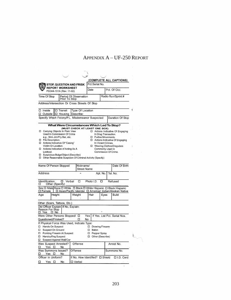
203

APPENDIX A – UF-250 REPORT

Neighborhood Disorganization and Police Decision-Making in ...

Documents

Transcript of Neighborhood Disorganization and Police Decision-Making in ...