NBA Expansion and Relocation: A Viability Study of …dougloudenback.com/nba/nba-analysis.pdf ·...

274 Rascher and Rascher

274

Journal of Sport Management, 2004, 18, 274-295© 2004 Human Kinetics Publishers, Inc.

NBA Expansion and Relocation:A Viability Study of Various Cities

Daniel RascherUniversity of San Francisco

Heather RascherSportsEconomics

An examination of possible expansion or relocation sites for the NBA is un-dertaken using a two-equation system requiring two-stage probit least squaresto estimate. The location model forecasts the best cities for an NBA teambased on the underlying characteristics of current NBA teams. The resultssuggest that Louisville, San Diego, Baltimore, St. Louis, and Norfolk appearto be the most promising candidates for relocation or expansion.

Regardless of the state of the economy, many cities continue to pursue big-league sports franchises for their metropolitan areas. For instance, Louisville hasbeen trying to lure a National Basketball Association (NBA) franchise for morethan 7 years. More recently, New Orleans successfully attracted the former Char-lotte Hornets to move into a new arena in the city.1 Both Northern Virginia andWashington, DC, are currently looking to house a Major-League Baseball (MLB)team. Moreover, Paul Allen was interested in bringing a National Hockey League(NHL) or MLB team to the city of Portland, WA, in an effort to provide content forhis regional sports network.

Professional basketball began in the United States in 1946 with 11 teams, 3of which are still in existence. Some teams have gone out of business; others havemoved to different cities and have changed names.2 Instances of relocation, how-ever, are infrequent. Some of the recent team relocations include the Golden StateWarriors’ move from San Francisco to Oakland (1971); the Rockets’ move fromSan Diego to Houston (1971); the Wizards’ move to Washington in 1974 (renamedthe Wizards in 1997 from the Washington Bullets); the Nets’ move to New Jersey(East Rutherford) from New York (1977); the Jazz’s move from New Orleans toSalt Lake City (1979); the Clippers’ move to Los Angeles from San Diego (1984);and the Kings’ move to Sacramento from Kansas City (1985).3 The Vancouver

D. Rascher is with the University of San Francisco, Sport Management Program,2130 Fulton Street, San Francisco, CA 94117-1080. H. Rascher is with SportsEconomics,110 Brookside Dr., Berkeley, CA 94705.

NBA Expansion 275

Grizzlies’ move in 2001 to Memphis (over cities such as Louisville, St. Louis, andNew Orleans) and the aforementioned Hornets’ move to New Orleans are the mostrecent relocations.

One key impetus for relocation is to increase arena-related team revenues.Some owners argue that the increased revenues from a new arena put a franchisein a better position to bid for quality players, resulting in a better team, which, inturn, draws more fans, resulting in more revenues, and so on. The type of sportsfacility and lease arrangements are as important as the quality of the market in anowner’s location decision.

For instance, in the NFL a few teams have recently relocated to smallermarkets in order to play in a new stadium with a “sweetheart” lease agreement, inwhich the teams are offered more favorable stadium deals in order to entice themto relocate. In 1995 the Raiders moved from Los Angeles (the second largest mar-ket in the U.S.) back to Oakland, and the Rams moved from Los Angeles to St.Louis. In 1996 the Browns moved to Baltimore to become the Ravens, and theOilers moved to Tennessee from Houston (becoming the Titans) the followingyear.4 In each of these cases, the new market was smaller (in terms of population)than the previous market. Moreover, the Hornets move from Charlotte to NewOrleans was primarily because of a more appealing facility agreement with NewOrleans for a state-of-the-art facility; the relocation, however, placed the team in asmaller media market and a less affluent city.5

Team relocations, and the threat thereof, have commensurately increasedthe value of major-league clubs. The Oakland A’s and Montreal Expos (MLB), theMinnesota Vikings (NFL), and numerous NHL franchises are also consideringnew locations. This is primarily because of the fact that the four major sports leaguescontrol the supply of teams, the placement of franchises, and the number of teamspermitted to locate in any market. In spite of demand, the leagues are reluctant toincrease the rate of expansion-team creation. In fact, since the NFL and AFL mergedin 1966, the NFL has added only seven additional teams, even though severalmarkets desire franchises.6

Which cities should teams choose when considering their ideal locale? Thechoice of a city depends on at least three major factors: the owner’s personal pref-erence, the political climate, and the economics of the location. Whereas manyteam owners are profit maximizers and make decisions accordingly, some ownersmight be more personally motivated, perhaps choosing to move a team to a citybecause it is where they live. For instance, Georgia Frontiere, owner of the St.Louis Rams, moved the team from Los Angeles to her hometown of St. Louis,MO. Similarly, the Minnesota Vikings are considering a move to San Antonio,TX, because owner Billy Joe “Red” McCombs is from San Antonio.7 Personalpreference, as in these cases, is idiosyncratic and will therefore not be investigatedin this analysis.

Political support for a major league team in a city is very important becausearenas and stadiums are often financed in part or in full by local governments.8 Thelocation decision is usually the result of a bidding competition among the govern-ments of various cities, each offering a variety amenities to the teams in order to


attract the team to their locale. In fact, the moves by the Oilers, Rams, and Raiderswere all to smaller markets, but the stadium leases were more favorable in thesemarkets, despite the reduced population of their new locations.

Finally, the economics of the market matters. Regions with larger, richerpopulations and those that contain large businesses or numerous corporate head-quarters are assumed to more readily support a team than a smaller city that lacksthese desirable demographic features. The three overarching decision criteria, how-ever, can be interrelated. For instance, the degree of public funding is likely tocorrespond to the size and economic demographics of the market. In fact, there isa correlation of .33 (significant at the 1% level) between the percentage of publicfunding and the population for six cities with NBA teams that are in relativelysmaller population centers. In addition, an owner’s preferences are likely to be infavor of locating in a large metropolitan area because of the potential favorableeconomics.

This article analyzes the economics of each potential market to determinewhich cities are likely to be the best prospects for expansion or relocation of NBAteams. A hierarchical two-equation system is employed. In the first equation of thelocation model, the 25 current U.S. markets that have NBA franchises are exam-ined to determine the relationship among the underlying factors.9 It is then used toforecast the relative likelihood of other cities being similar enough to NBA citiesto be able to support a team (again based on economic factors, not personal prefer-ence or political factors). This model is similar to the analysis for baseball teamsby Bruggink and Zamparelli (1999) except that the NBA model has additionalvariables, two stages, and uses a substantially different econometric approach.

The second equation is a revenue equation. The revenue forecasts generatedare used as inputs into the first equation. The logic is that the potential revenueseach location could generate are important factors in an owner’s location decision.

One objective of the overall analysis is to be able to aid in the financialdecision regarding league expansion or team relocation. The current methodologyused in the field involves separate comparisons of cities by population and a fewother measures, as opposed to an integrated approach that captures the relation-ships between the factors and relative importance of each. A set of models such asdescribed in this article can be used to rank cities for further, more in-depth analy-sis across many sports and in many countries.

The next section examines the basic theory underlying the analysis. Thedata, data sources, and limitations are described in the third section. The analysisand results for the two-equation system is presented in the fourth section, and thefinal section provides a summary and a discussion of the results.

Theoretical Model

The location model is a franchise model based on the work, most recently, ofBenjamin Klein (1995). Owners of franchises in the same company have the in-centive and desire to locate at least some minimum geographic distance away fromeach other, but want to maintain similarity in terms of quality and products offered

NBA Expansion 277

in order to reduce uncertainty for customers. For instance, Domino’s Pizza fran-chises are not allowed to locate near each other unless they are owned by the samefranchisee.

Sports teams (or franchises) operate in a similar manner, and each of theleagues has developed rules regarding franchise movement and location. In theNBA, an area with a radius of 75 miles surrounds each NBA team, and no otherNBA team is permitted to locate within that radius without permission of the in-cumbent team. To understand the rationale as to why NBA teams chose their cur-rent locations, the location model takes into consideration the information avail-able from current teams and uses that data to determine the common underlyingeconomic factors of existing NBA locations. The cities currently without NBAteams are then evaluated based on those factors. In order to discern between suc-cessful locations of current NBA teams and less successful ones, the revenue equa-tion in the location model accounts for the relative success of each location.

The general model is Location = f (market characteristics, revenue poten-tial, political support, owner preferences) and Revenue Potential = g (market char-acteristics, team characteristics). Market characteristics contain variables such aspopulation, income, competition from other sports teams, basketball fanaticism,and corporate depth. Team characteristics contain variables such as prices, win-ning percentage, and arena quality. The relationship that results from revenue po-tential is an input into the location relationship. This creates a hierarchical, two-equation system. Owner preferences are excluded from the models because theyare based on where an owner would like to locate a team and determining this isabove and beyond the scope of this study.

Similarly, there are difficulties in trying to model political support. For onething, the political support for constructing an NBA arena in a city without anNBA team might not be revealed in any data available if the issue has not previ-ously arisen. Information on political support for other major professional sportsteams might be a useful, comparable variable, but many of these cities do not haveany other major professional sports teams. In addition, if a city has already spent alarge sum of public money to build a baseball stadium, it is often unclear whetherit would be more or less likely to finance an NBA arena with public funds.

Another avenue in modeling potential political support is to note whetherpolitical leaders account for the public’s preferences when spending public money,or if the public votes directly on the issue. If the public votes on the issue, then ameasure of the public’s preferences towards basketball might be informative. Anexplanatory variable of the location model, basketball fanaticism, might capturethe public’s likely support for publicly financing an arena. In fact, there is a corre-lation of –0.2323 between the existing degree of public support for current arenas(in those cities with an NBA team) and the basketball fanaticism ranking (whichmeans a higher score = less fanatical, and it is significant at the 5% level).10

Further, cities with higher populations (another of the explanatory variables in themodel) are more likely to publicly fund an arena.11 Therefore, basketball fanati-cism and population partially capture the degree of political support that an ownermight expect to receive in each potential location.


In summary, the theoretical model is a two-equation system measuringwhether a city is a good or poor candidate for an NBA team. A testable assumptionis that NBA cities that maintain a team over a long period of time have factors incommon. For example, the empirical analysis will determine the importance ofpopulation as a common factor that successful NBA teams share.

The two-equation system representing the model is as follows:

Y1 = αY

2 + β

1X

1 + µ

1

Y2 = β

2X

2 + µ

2

where Y1 is a binary variable, X

1and X

2 are vectors of independent variables, µ

1 and

µ2 are error terms, α

and β

i (i = 1, 2) are vectors of parameters to be estimated, and

Y2 is a continuous variable. Equation 2 is a revenue equation based on the triangu-

lar hierarchical structure and feeds into Equation 1, the location equation. Y1 takes

a value of 1 if the city contains an NBA team, and 0, otherwise. The error terms, µ1

and µ2, are not uncorrelated because Y

2 is correlated with µ

2, and, given that Y

2 is

part of equation 1, µ2 is correlated with µ

1.

Equation 1 models cities that currently have NBA franchises based on X1

(market characteristics) and Y2 (a forecast of potential revenue for an NBA team in

that location). Equation 2 is a forecast equation that is an input into Equation 1. Itis explained by factors in X

2, such as market characteristics and team characteris-

tics, that affect the revenue of NBA teams.

Data

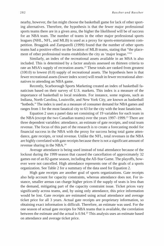
The cross-sectional data for Equation 1 of the location model consists of 48observations from 1999 (unless otherwise specified): 25 are for cities with NBAteams, and 23 are for cities without NBA teams that are potentially the most eli-gible cities for league expansion or team relocation.12 There are 12 potential ex-planatory variables, some of which are correlated (e.g., 1995 metropolitan statiscalarea [MSA] population and 2000 MSA population).13 Each observation representsinformation for the year 1999 (except where specified).

The dependent variable in Equation 1, Y1, is an indicator or dummy variable

that distinguishes a city with an NBA team (or two) from a prospective NBA citywithout a team for the 1999 season.

In developing a forecasting model for possible locations for NBA teams, it isimperative to include the population of the market for each team. Five populationvariables are examined: 1990 city population, 1999 city population, MSA popula-tion for the years 1995 and 2000, and the MSA population growth over that pe-riod.14 It is likely that an NBA team draws not only from the city in which it islocated but also from the surrounding towns and communities. Therefore, the MSApopulation is expected to provide the best relative forecast of the populationvariables. It is expected that the effect of population on whether a city has or at-tains an NBA team will be positive. A summary of the data is provided in Table 1.

(1)

(2)

NBA Expansion 279

Tab

le 1

Sim

ple

Stat

isti

cs o

f th

e N

BA

Rev

enue

Mod

el D

ata

Min

imum

Mea

nM

edia

nM

axim

umSt

d. d

ev.

Dep

ende

nt v

aria

ble:

avg.

atte

nden

ce a

t gam

es9,

968

17,0

7517

,072

23,9

882,

927

estim

ated

gat

e re

ceip

ts o

f ea

ch te

am’s

hom

e ga

mes

($)

19,3

79,8

9234

,547

,708

33,5

01,6

7869

,567

,390

11,7

00,0

00to

tal r

even

ue (

mill

ions

of

$)34

.570

.767

.415

2.2

24.3

Inde

pend

ent v

aria

bles

:ar

ena

seat

cap

acity

16,3

1119

,586

19,6

0024

,042

1,64

7ye

ar s

easo

n be

gan

1997

1998

1998

1999

0.82

avg.

tick

et p

rice

($)

23.6

944

.01

43.0

986

.82

12.3

7co

nces

sion

s pr

icea (

$)6.

008.

908.

7511

.75

1.21

avg.

bee

r pr

ice

($)

2.50

4.10

4.00

6.00

0.63

avg.

hot

dog

pri

ce (

$)1.

002.

502.

504.

000.

51av

g. s

oda

pric

e ($

)1.

502.

302.

254.

500.

47to

tal p

rice

b ($)

36.4

461

.30

58.0

012

3.32

15.9

4

(con

tinu

ed)


avg.

par

king

pri

ce (

$)0.

008.

387.

0027

.00

4.71

bask

etba

ll fa

natic

ism

inde

x1.

022

.016

.059

.016

.9re

crea

tiona

l ind

ex r

anki

ng65

.788

.189

.899

.78.

7nu

mbe

r of

oth

er m

ajor

spo

rts

team

s lo

cate

din

city

0.0

2.1

2.0

7.0

1.8

MSA

hou

seho

ld in

com

e ($

)68

,000

83,0

8983

,400

100,

203

9,25

2M

SA p

opul

atio

n, 2

000

1,25

3,52

33,

763,

065

2,89

1,59

59,

187,

860

2,58

3,40

5m

idsi

zed

corp

orat

ions

in M

SA84

23,

565

3,30

08,

267

2,49

7la

rge

corp

orat

ions

in M

SA39

51,

814

1,73

34,

115

1,27

6fo

rtun

e 50

0 co

mpa

nies

hea

dqua

rter

ed in

MSA

0.0

13.0

11.0

52.0

13.5

cost

of

livin

g in

dex

rank

ing

0.0

25.0

21.3

91.8

23.2

team

win

ning

per

cent

age

0.13

0.51

0.54

0.82

0.16

prev

ious

sea

son

team

win

ning

per

cent

age

0.13

0.52

0.54

0.84

0.17

num

ber

of a

ll–st

ar v

otes

rec

eive

d20

,631

925,

597

601,

359

5,59

7,84

21,

045,

122

age

of a

rena

1.0

11.2

8.0

39.0

10.5

dist

ance

to n

eare

st c

ity w

ith N

BA

fra

nchi

se81

.621

6.3

181.

353

3.0

126.

7

a Con

cess

ions

pri

ce =

tota

l of

beer

, hot

dog

, and

sod

a pr

ices

.b Tot

al p

rice

= to

tal o

f co

nces

sion

, tic

ket,

and

park

ing

pric

es. M

SA =

met

ropo

litan

stat

isca

l are

a.

Tab

le 1

(con

tinu

ed)

Min

imum

Mea

nM

edia

nM

axim

umSt

d. d

ev.

NBA Expansion 281

The growth of a community could play a role in whether an NBA team choosesto locate there, especially if annual growth is significant and consistent. The growthvariable is the change in MSA population during the past 5 years. The expectedeffect is that a higher population growth rate will increase the probability of anNBA team choosing to locate in a particular area. Alternatively, a city that has asignificant decline in population might decrease the probability of an NBA teamchoosing to locate there.

Typical household income and average pay per worker of the MSA are alsoincluded as potential determining factors of NBA franchise location.15 Other stud-ies have found income to be a significant factor in determining attendance at sport-ing events.16 As for location of sports teams, Bruggink and Zamparelli (1999) foundthat a $1,000 increase in average household income increased the probability ofthe city having a MLB team by 8%. The expected effect is that a higher typicalhousehold income in an MSA will increase the probability of an NBA team choos-ing that location.

Similarly, a measure of the relative cost of living in these metropolitan areasis considered in order to obtain a reasonable measure of household disposableincome. The cost-of-living index takes into consideration nine items that collec-tively represent more than 60% of the typical household budget, which varies widelyamong regions.17 The annual costs for these items were ranked from lowest tohighest and then scored such that 100.00 represents the least expensive, 50.00indicates the median, and 0.00 ranks as the most expensive city. The theory here isthat regions with higher disposable income might choose to allocate a higher per-centage of their budget towards recreational and leisure activities such as attend-ing an NBA game.

The success of sports teams in the modern era is largely dependent on corpo-rate support via the purchase of luxury suites, club seats, sponsorship (includingnaming rights), and other premium services. The locational analysis includes ameasure of corporate supply by using the number of Fortune 500 companies thatare headquartered in a relevant city.18 Although not a perfect measure of corporatesupply, it is expected that large corporations might want to entertain clients oremployees in the luxury suites of a professional sports franchise located in the cityin which they are headquartered. Also included are two measures of the number ofcompanies that are considered to be large enough to be interested in premiumservices, such as luxury seats, and profitable enough to be able to afford suchservices.19

As in any spatial model of competition, the distance between competitorscan affect the success of a business. The distance in miles to the nearest city withan NBA team is used as a measure of spatial competition. All else equal, it isexpected that franchises located relatively far distances from other franchises havea higher likelihood of success.20

Competitors to a sports franchise would be any other major professionalsports teams located in the same area. For instance, a sports fan might choose toattend a hockey game instead of a basketball game. If there was no hockey team


nearby, however, the fan might choose the basketball game for lack of other sport-ing alternatives. Therefore, the hypothesis is that the fewer major professionalsports teams there are in a given area, the higher the likelihood will be of successfor an NBA team. The number of teams in the other major professional sportsleagues (NHL, NFL, and MLB) is used as a proxy for sports-entertainment com-petition. Bruggink and Zamparelli (1999) found that the number of other sportsteams had a positive effect on the location of MLB teams, stating that “the place-ment of other professional teams establishes the city as ‘major league.’”21

Similarly, an index of the recreational assets available in an MSA is alsoincluded. This is determined by a factor analysis assessed on thirteen criteria torate an MSA’s supply of recreation assets.22 These totals are ranked from greatest(100.0) to lowest (0.0) supply of recreational assets. The hypothesis here is thatfewer recreational assets (lower index score) will result in fewer recreational alter-natives to attending an NBA game.

Recently, Scarborough Sports Marketing created an index of basketball fa-naticism based on their survey of U.S. markets. This index is a measure of theimportance of basketball to local residents. For instance, some regions, such asIndiana, North Carolina, Louisville, and New York City, are known as basketball“hotbeds.” The index is used as a measure of consumer demand for NBA games andranges from 1 for the most fanatical city to 63 for the city with the least fanaticism.

Equation 2 uses a panel data set consisting of 19 variables for each team inthe NBA (except the two Canadian teams) over the years 1997–1999.23 There arethree dependent variables: attendance, an estimate of gate receipts, and total teamrevenue. The focus of this part of the research is to create a forecasting model forfinancial success in the NBA with the proxy for success being total game atten-dance, gate receipts, or total revenue. Unlike the NFL, total revenues in the NBAare highly correlated with gate receipts because there is not a significant amount ofrevenue sharing in the NBA.24

Average attendance is being used instead of total attendance because of thelockout during the 1999 season that caused the cancellation of approximately 32games out of an 82-game season, including the All-Star Game. The playoffs, how-ever were not cancelled. High attendance represents one of the goals of a sportsorganization. See Table 2 for a summary of the data used for Equation 2.

High gate receipts are another goal of sports organizations. Gate receiptsalso help account for capacity constraints, whereas attendance does not. For in-stance, smaller arenas can charge higher prices if the supply of seats is less thanthe demand, mitigating part of the capacity constraint issue. Ticket prices varysignificantly across teams, and, by using only attendance, this price informationwould be lost. Gate receipts are estimated using actual attendance and averageticket price for all 3 years. Actual gate receipts are proprietary information, soobtaining exact information is difficult. Therefore, an estimate was used. For theone season of actual gate receipts for NBA teams that is available, the correlationbetween the estimate and the actual is 0.94.25 This analysis uses an estimate basedon attendance and average ticket price.

NBA Expansion 283

Tab

le 2

Sim

ple

Stat

isti

cs o

f th

e N

BA

Loc

atio

n M

odel

Dat

a

Min

imum

Mea

nM

edia

nM

axim

umSt

d. D

ev.

Dep

ende

nt v

aria

ble

NB

A te

am lo

cate

d in

city

0.00

0.52

1.00

1.00

0.50

Inde

pend

ent v

aria

bles

MSA

pop

ulat

ion

grow

th, 1

995–

2000

–1.2

%5.

9%5.

1%21

.6%

4.7%

MSA

pop

ulat

ion,

200

071

2,46

02,

451,

255

1,61

9,45

09,

220,

312

1,94

7,82

1M

SA p

opul

atio

n, 1

995

669,

998

2,34

0,97

71,

629,

508

9,05

4,39

41,

923,

162

bask

etba

ll fa

natic

ism

inde

x1.

027

.226

.063

.018

.6M

SA h

ouse

hold

inco

me

($)

52,7

0077

,935

77,1

5010

0,20

310

,393

num

ber

of o

ther

maj

or s

port

s te

ams

loca

ted

in c

ity0.

01.

52.

07.

01.

5fo

rtun

e 50

0 co

mpa

nies

hea

dqua

rter

ed in

MSA

0.0

8.4

4.0

52.0

9.3

mid

size

d co

rpor

atio

ns in

MSA

289

2,19

01,

612

8,26

71,

975

larg

e co

rpor

atio

ns in

MSA

153

1,11

376

24,

115

1,03

6re

crea

tiona

l-in

dex

rank

ing

42.5

85.1

87.5

100.

010

.9co

st-o

f-liv

ing–

inde

x ra

nkin

g0.

036

.135

.095

.525

.3av

g. N

iels

en T

.V. r

atin

gs f

or N

BA

gam

esin

city

0.9

2.6

2.0

6.9

1.61

avg.

Nie

lsen

T.V

. rat

ings

for

6 N

BA

gam

esin

city

1.5

4.6

4.2

13.1

2.25

dist

ance

to n

eare

st c

ity w

ith N

BA

fra

nchi

se45

274

194

2,56

036

1

Not

e. M

SA =

met

ropo

litan

sta

tistic

al a

rea.


The third measure of revenue is total team revenue as reported by Forbesmagazine. Other localized revenue sources not included in gate receiptssuch as media, sponsorship, concessions, and parking are included in thisfigure.

The independent variables used to predict financial success or to measureattendance demand are prices, team winning percentage, a measure of the quantityof star players, the age of the venue, the year of the season, basketball fanaticism,household income, number of other professional sports teams located in the MSA,2000 MSA population, recreational and cost-of-living indices, number of Fortune500 companies headquartered in MSA, the number of midsized and large corpora-tions in MSA, and distance to nearest NBA city.

There is also a vector of prices that fans pay to attend sporting events. Theseinclude the ticket price, the price of a 12-oz beer, the price of a hot dog, the price ofa 12-oz soda, and the price of parking.26 The first law of demand predicts thathigher prices will lead to lower levels of demand, ceteris paribus. Ticket pricesaverage $44 for the sample, with a low of $24 and a high of $87.

Winning percentage is expected to be an important proxy for the quality ofthe home team. The winning percentage in the year each season began for 1997through 1999 was used.27 Many studies have found winning to be an impor-tant determinant of attendance demand.28 As expected, the average winningpercentage is near .500 (at .514), with the minimum at .134 and the maximumat .817.29

Lagged winning percentage is also expected to affect demand because theprevious season’s performance affects season ticket sales and the appeal of earlyseason games. For instance, Rascher (1999) shows that, in baseball, an extra winby the home team in the previous season increases per-game attendance by about450 fans for the first half of the season, but by the second half of the season, theincrease declines in magnitude to 150 fans per game (signfigance declines, as well,with the t statistic dropping from 7.64 to 3.02).

Relative to other major professional sports, the NBA markets its product byfocusing on the individual talent of the players more so than the quality of eachteam. It is expected that the star power of the players on a team will affect thedemand for games above and beyond their skill in producing wins. The analysisuses the number of all-star votes that each team received as a proxy for the indi-vidual star power of each team.

Sports teams in the U.S. have been on a facility-construction spree in the lastdecade. The older domes built in the late 1960s and early 1970s have given way tonewer, higher quality, entertainment-oriented facilities. These facilities increasethe revenue streams for NBA and NHL teams by as much as 50% because theyoffer better amenities including premium seating, parking, food, drink, and non-game entertainment. In MLB, a new stadium can generate more than $40 millionin new revenue annually.30 The analysis uses the age of the sports venue as a proxyfor the quality of fans’ experiences unrelated to the game. The remaining variableswere described earlier.

NBA Expansion 285

Analysis and Results

The location model creates a forecast of the best cities for NBA expansion orrelocation based on economic factors that exist in current NBA cities. The depen-dent variable, whether the city has an NBA team, is an indicator variable. Themodel is a two-equation system with a binary dependent variable and a continuousendogenous variable. The type of triangular system described in the section on thetheoretical model requires a two-stage probit least squares (2SPLS) estimationtechnique.

The first stage is the estimation of Equation 2, the revenue equation. Typi-cally, ordinary least squares (OLS) estimation would be unbiased and efficient,but there are a few econometric issues that prevent straight OLS from working.First, the revenue equation is estimated using data for 27 teams over 3 years. Theerror structure exhibits cluster correlation. For each team, the error term for 3years is autocorrelated. Even though there is not correlation across teams, there iscorrelation of the errors within each team. The effect of cluster correlation is toinflate t statistics. In this case, the t statistics are about 12% higher when not ac-counting for the cluster correlation problem. The solution involves estimating ro-bust errors by analyzing a cluster variable in the model itself.

The second estimation problem is that one of the dependent variables, atten-dance, is censored because of the capacity constraint of the size of an arena. Truedemand might be larger than actual attendance, but the size of the arena preventsthe full demand from being satisfied. Interval regression offers a solution in thetradition of Tobit (Tobin, 1958).

In calculating the correlation between each of the variables, income and popu-lation, as expected, are correlated—people in larger cities have higher incomes.Another multicollinearity issue occurs among population, the number of corporateheadquarters, and the number of non-NBA sports teams. The smallest bivariatecorrelation among these variables is .73. Although it is not surprising that corpora-tions and sports teams locate in large population centers, the interpretation of theindividual effects of these factors on NBA team location could be inefficient, butnot biased, if included simultaneously in econometric analysis. Because the goalin this step of the analysis is not to interpret individual effects but to create anendogenous variable to be used in the next step, these variables were included inthe analysis.

Sensitivity analyses showed that there was no omitted variable bias. Evi-dence of heteroscedasticity was accounted for using White’s corrected errors. Log-linear models were estimated, but the levels models had superior fit. Log-linearmodels are often used in demand estimation, but only because the elasticities areeasy to calculate. In this case that reason is not compelling enough to use log-linear models. Table 3 shows the results of the revenue and attendance equationsestimation.

Overall, the attendance model is extremely statistically significant with aWald χ2 statistic of 74.14. Both the gate-receipts and total-revenue models have R2

values greater than 0.53 and F values that are significant at the 1% level. Each of


Table 3 Attendance and Revenue Regression Results

Total revenueModel Attendance Gate receipts in millions

Adjusted R2 — 0.55 0.53F-value or Wald Chi2 74.14*** 13.42*** 7.86***Number of observations 81 81 81Independent variables

constant 1447.55 –39,100,000** –24.4(0.19) (–2.14) (–0.56)

basketball fanaticism index –91.06*** –319,263*** –0.35(–3.28) (–4.38) (–1.62)

number of other major sports 405.40 1,209,033 2.79teams located in city (1.12) (0.82) (0.70)

population of local MSA 0.0000485 1.71 0.0000031(0.10) (1.39) (1.09)

index of recreation opportunities 27.09 118,218 0.26(0.75) (1.15) (1.06)

MSA household income 0.1490* 680.2*** 0.00044(1.67) (3.26) (0.95)

number of midsized companies –0.924 –4208* 0.00034in MSA (–0.74) (–1.76) (0.06)

current season winning 1451.47 9,033,650 36.53*percentage (0.52) (0.87) (1.72)

previous season team winning 8136.83*** 13,500,00*** 22.96**percentage (4.02) (2.82) (1.97)

age of arena –73.06 –235,793* –0.52(–1.37) (–1.65) (–1.62)

Note. Significance:* = 10% level; ** = 5% level; *** = 1% level. MSA = metropolitanstatistical area. T statistic in parentheses.

the Stage-1 models is statistically significant and provides suitable endogenousvariables for Stage 2. Basketball fanaticism, household income, previous season’swinning percentage, and age of the arena are consistently statistically significantwith the expected signs.31 Interpreting the marginal impacts of a few of the vari-ables that do not suffer from multicollinearity, a 5% increase in household incomeis associated with an 8% increase in gate receipts. An increase of 10% in gameswon (e.g., from 0.500 to 0.600—eight more wins) is associated with a rise in gatereceipts of 4%, or $1.35 million. The aging of a stadium is associated with lowergate receipts, about $235,000 per year.

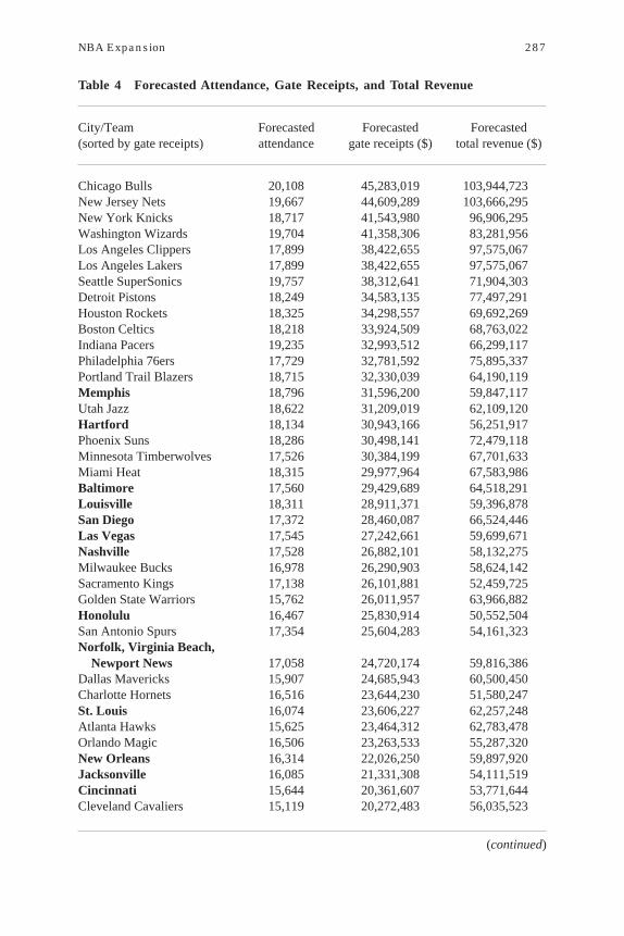
Table 4 shows the forecasts of attendance, gate receipts, and total revenuefor each NBA and non-NBA city, sorted by decreasing gate receipts.32 Gate re-ceipts range from a high of $84 million in Chicago, down to $32 million in El

NBA Expansion 287

Table 4 Forecasted Attendance, Gate Receipts, and Total Revenue

City/Team Forecasted Forecasted Forecasted(sorted by gate receipts) attendance gate receipts ($) total revenue ($)

Chicago Bulls 20,108 45,283,019 103,944,723New Jersey Nets 19,667 44,609,289 103,666,295New York Knicks 18,717 41,543,980 96,906,295Washington Wizards 19,704 41,358,306 83,281,956Los Angeles Clippers 17,899 38,422,655 97,575,067Los Angeles Lakers 17,899 38,422,655 97,575,067Seattle SuperSonics 19,757 38,312,641 71,904,303Detroit Pistons 18,249 34,583,135 77,497,291Houston Rockets 18,325 34,298,557 69,692,269Boston Celtics 18,218 33,924,509 68,763,022Indiana Pacers 19,235 32,993,512 66,299,117Philadelphia 76ers 17,729 32,781,592 75,895,337Portland Trail Blazers 18,715 32,330,039 64,190,119Memphis 18,796 31,596,200 59,847,117Utah Jazz 18,622 31,209,019 62,109,120Hartford 18,134 30,943,166 56,251,917Phoenix Suns 18,286 30,498,141 72,479,118Minnesota Timberwolves 17,526 30,384,199 67,701,633Miami Heat 18,315 29,977,964 67,583,986Baltimore 17,560 29,429,689 64,518,291Louisville 18,311 28,911,371 59,396,878San Diego 17,372 28,460,087 66,524,446Las Vegas 17,545 27,242,661 59,699,671Nashville 17,528 26,882,101 58,132,275Milwaukee Bucks 16,978 26,290,903 58,624,142Sacramento Kings 17,138 26,101,881 52,459,725Golden State Warriors 15,762 26,011,957 63,966,882Honolulu 16,467 25,830,914 50,552,504San Antonio Spurs 17,354 25,604,283 54,161,323Norfolk, Virginia Beach,

Newport News 17,058 24,720,174 59,816,386Dallas Mavericks 15,907 24,685,943 60,500,450Charlotte Hornets 16,516 23,644,230 51,580,247St. Louis 16,074 23,606,227 62,257,248Atlanta Hawks 15,625 23,464,312 62,783,478Orlando Magic 16,506 23,263,533 55,287,320New Orleans 16,314 22,026,250 59,897,920Jacksonville 16,085 21,331,308 54,111,519Cincinnati 15,644 20,361,607 53,771,644Cleveland Cavaliers 15,119 20,272,483 56,035,523

(continued)


Paso, TX. Based on these Stage-1 results (revenues), the best cities for expansionor relocation are Memphis, Hartford, Baltimore, Louisville, San Diego, Las Ve-gas, and Nashville.

The second stage of the 2SPLS involves the estimation of Equation 1 withthe estimated dependent variable from Equation 2 as an endogenous variable inthe model. Again, the attendance, gate receipts, and total revenue estimates fromTable 3 are regressors in the estimation of Equation 2. A number of sensitivity testswere performed on the model before final selection. Scatter plots and the Cook-Weisberg test show that heteroscedasticity is an issue with the data. White’s cor-rected errors are used to avoid inflated t statistics from heteroscedasticity. Thereappears to be one or more omitted variables based on the results of the RamseyRESET test.

Table 5 shows the results of the probit analysis. Overall, the models aresignificant at the 5% or better level. Interpretation of the marginal impacts showsthat a 10% increase in attendance, gate receipts, or total revenue is associated withan 11%, 10%, and 17% increase in the probability that a city is suitable for an NBAteam, respectively.

Conclusion and Discussion

The forecasts for which cities are “best” for NBA expansion or relocationare shown in Table 6. Louisville and San Diego lead the list of potential candi-dates. This model examines the underlying economic structure of the cities in or-der to create forecasts for expansion or relocation of NBA teams. Models of thistype could be used for many other sports and in other regions and countries.

Austin–San Marcos 15,931 19,766,609 49,390,583Denver Nuggets 14,939 19,541,896 51,326,220Kansas City 15,280 19,503,955 54,329,534Albuquerque 15,394 17,362,572 45,547,891Columbus 13,879 13,684,159 45,976,470Pittsburgh 13,357 12,543,029 48,788,601Omaha 13,553 12,345,181 39,255,986Buffalo–N. Falls 13,659 11,974,656 46,414,481Oklahoma City 11,432 11,114,854 33,726,430Tucson 11,071 10,608,078 31,618,100El Paso 9,311 10,178,875 19,506,282

Note. Bolded cities are those without an NBA team in 1999.

Table 4 (continued)

City/Team Forecasted Forecasted Forecasted(sorted by gate receipts) attendance gate receipts ($) total revenue ($)

NBA Expansion 289

Before the 2001–2002 season, the Vancouver Grizzlies of the NBA had tomake a location decision. The team decided to move out of Canada and created ashort list of possible locations that they believed could sustainably and success-fully support the franchise. San Diego, Las Vegas, New Orleans, Memphis, andLouisville were on the list. The city of San Diego showed no interest in the Griz-zlies because, at the time, the city was embroiled in a dispute over a half-built,publicly financed baseball stadium. The NBA ruled out the city of Las Vegas be-cause of its ties to gambling. St. Louis had been a contender the year before thesale, but after the failed purchase of the team by St. Louis Blues (NHL) owner BillLaurie, he declared he would not open the Savvis Center to a an NBA team ofwhich he was not the owner. The three final locations were quickly narrowed totwo, because New Orleans was unable to generate an offer that was suitable to theGrizzlies. The decision between Memphis and Louisville was tipped in favor ofMemphis when Federal Express (FedEx), whose headquarters are in Memphis,made a naming rights offer and equity purchase of the team.33 The results heresupport the location decision made by the Grizzlies.

More recently, the Hornets considered Louisville, Norfolk, VA, and NewOrleans for their relocation out of Charlotte before agreeing to terms with NewOrleans. Based on the findings in this study, the Hornets might have been betteroff moving to Louisville. This is supported by the fact that attendance last seasonin New Orleans was below expectations.

Changes in the revenue-generating capability of sports facilities are amongthe most important factors that have improved the profitability of sports-team fran-chises recently. All four of the major professional sports leagues have recentlyseen an increase in the variance of team valuations because the team owners retain

Table 5 Two–Stage Probit Least Squares Results

NBA indicator NBA indicator NBA indicatorModel variable variable variable

Wald Chi–Square 5.84** 12.66*** 9.86***Number of Observations 45 45 45Independent Variables

constant –3.30** –3.16*** –5.95***(–2.21) (–3.08) (–2.98)

attendance from stage one 2.14e-4*** 1.15e-7*** ––(2.42) — ––

gate receipts from stage one –– (3.56) 0.0855***total revenue from stage one –– –– (3.14)

Note. Significance: * = 10% level; ** = 5% level; *** = 1% level. T statistic in parentheses.


Table 6 Forecast Results for Location Model Predicting Probable NBA Cities

Forecasted Forecasted ForecastedCity/Team probability probability probability(sorted by gate receipts) (attendance) (gate receipts) (total revenue)

Atlanta Hawks 1.000 1.000 1.000Boston Celtics 1.000 1.000 1.000Chicago Bulls 1.000 1.000 1.000Dallas Mavericks 1.000 1.000 1.000Detroit Pistons 1.000 1.000 1.000Houston Rockets 1.000 1.000 1.000Los Angeles Lakers 1.000 1.000 1.000Los Angeles Clippers 1.000 1.000 1.000Minnesota Timberwolves 1.000 1.000 1.000New York Knicks 1.000 1.000 1.000New Jersey Nets 1.000 1.000 1.000Golden State Warriors 1.000 1.000 1.000Philadelphia 76ers 1.000 1.000 1.000Washington Wizards 1.000 1.000 1.000Portland Trail Blazers 1.000 1.000 1.000Seattle SuperSonics 0.997 0.998 0.990Phoenix Suns 0.937 0.989 0.947Utah Jazz 0.963 0.962 0.912Charlotte Hornets 0.919 0.954 0.896Indiana Pacers 0.873 0.953 0.901Orlando Magic 0.816 0.862 0.817Louisville 0.740 0.743 0.751Milwaukee Bucks 0.501 0.709 0.520Denver Nuggets 0.675 0.707 0.715San Antonio Spurs 0.404 0.703 0.549San Diego 0.696 0.677 0.658Miami Heat 0.675 0.585 0.615Las Vegas 0.416 0.345 0.442Baltimore 0.252 0.288 0.256St Louis 0.271 0.279 0.299Cleveland Cavaliers 0.351 0.262 0.323Norfolk, Virginia Beach,

Newport News 0.220 0.255 0.352Memphis 0.486 0.241 0.331Pittsburgh 0.333 0.163 0.328Hartford 0.209 0.155 0.164Nashville 0.125 0.115 0.152Sacramento Kings 0.130 0.107 0.087

(continued)

NBA Expansion 291

much of facility revenues. Although the size and magnitude of a team’s market isimportant in determining its revenue-generating ability in the league, facility eco-nomics has quickly caught up with market size in determining financial success,as evidenced by the recent franchise moves and the awarding of a new NFL fran-chise to Houston over Los Angeles.

The major determinants of the profitability of any major professional sportsfranchise are the type of lease agreement it has and the quality of its stadium.Hence, an important aspect of the location decision is not only the underlyingeconomics of the market but also the actual lease agreement offered to a team byeach city. In other words, if the market economics are better in a larger city, modelsof this sort can help determine how much better a lease agreement has to be froma smaller city in order to convince an owner to move to the smaller city.34

If an expansion team were considering a larger market such as Kansas City(population of 1.8 million), for example, versus a smaller market such as Buffalo(population of 1.2 million), the model forecasts that a Kansas City team wouldgenerate about $8 million more per year in total revenue (about 17% more) thanwould a team in Buffalo. In order for a team to move to Buffalo, the lease agree-ment would have to include at least $8 million more per year in expected revenuefor the team. For instance, the combination of lower rent, property tax, sales tax,percentages of parking, concessions, etc. that the team keeps would have to add upto at least $8 million more than the lease in Kansas City offered.

In a real example, in choosing New Orleans over Louisville, the Hornetsassessed expected attendance, gate receipts, and total revenues. According to thefindings here, expected total revenues were about the same, but attendance andgate receipts were forecasted to be higher in Louisville than in New Orleans.

Austin – San Marcos 0.073 0.055 0.118Kansas City 0.017 0.015 0.036Cincinnati 0.003 0.001 0.004New Orleans 0.002 0.000 0.004Columbus 0.002 0.000 0.004Jacksonville 0.000 0.000 0.000Albuquerque 0.000 0.000 0.000Buffalo – N.Falls 0.000 0.000 0.000

Note. Bolded cities are those without an NBA team in 1999.

Table 6 (continued)

Forecasted Forecasted ForecastedCity/Team probability probability probability(sorted by gate receipts) (attendance) (gate receipts) (total revenue)


Presumably, the lease agreement in New Orleans accounted for the difference inforecasted gate receipts between the two possible locations.

In choosing Memphis over New Orleans, Louisville, St. Louis, Las Vegas,and San Diego, the Grizzlies chose the market with the highest expected atten-dance and gate receipts but not the highest total revenue. As described earlier inthis article, however, San Diego was not in a position to offer to build a new facil-ity and the owner of the Savvis Center in St. Louis was not interested in having anNBA team in the facility unless he owned it.

By using a hierarchical, two-equation system involving the underlying eco-nomic factors that are deterministic for a team’s success, this article provides amodel that aids in the financial decision regarding league expansion or team relo-cation. This integrative approach effectively captures inter-relationships amongfactors, as well as the relative importance of each factor. A set of models such asdescribed in this article are not solely applicable to NBA franchise location deci-sions but can also be used to rank cities for further, more in-depth analysis acrossmany sports and in many countries.

References

Baim, D.V., & Sitsky, L. (1994). The sports stadium as a municipal investment. Westport,CT: Greenwood Publishing Group.

Bruggink, T.H., & Zamparelli, J.M. (1999). Emerging markets in baseball: An econometricmodel for predicting the expansion teams’ new cities. In J. Fizel, E. Gustafson, & L.Hadley (Eds.), Sports economics: Current research (pp. 49-59). Westport, CT: PraegerPress.

Burdekin, R.C., & Idson, T.L. (1991). Customer preferences, attendances and the racialstructure of professional basketball teams. Applied Economics, 23, 179-186.

CSL, Inc. (1999). Feasibility study for baseball in Washington D.C. Unpublished report.Hausman, J.A., & Leonard, G.K. (1997). Superstars in the National Basketball Association:

Economic value and policy. Journal of Labor Economics, 15(4), 586-624.Hoang, H., & Rascher, D.A. (1999). The NBA, exit discrimination, and career earnings.

Industrial Relations, 38(1), 69-91.Klein, B. (1995). The economics of franchise contracts. Journal of Corporate Finance,

Contracting, Governance, and Organization, 2(1-2), 9-37.McDonald, M., & Rascher, D.A. (2000). Does bat day make cents?: The effect of

promotions on the demand for baseball. Journal of Sport Management, 14(1),8-27.

Rascher, D.A. (1999). A Test of the optimal positive production network externality in MajorLeague Baseball. J. Fizel, E. Gustafson, & L. Hadley (Eds.), Sports economics: Cur-rent research (pp. 27-45). Westport, CT: Praeger Press.

Rich, W.C. (2000). The economics and politics of sports facilities. Westport, CT: QuorumBooks.

Savageau, D. With D’Agostino, R. (2000). Places Rated Almanac (millennium ed.). FosterCity, CA: IDG Books Worldwide, Inc.

Tobin, J. (1958). Estimation of relationships for limited dependent variables. Econometrica.26, 24-36.

NBA Expansion 293

Notes

1The third time was a charm for New Orleans. Since losing the Jazz to Utah in 1979,the city had twice attempted to land an NBA team. The NBA blocked an attempt to bring theMinnesota Timberwolves to New Orleans in 1994, and the Vancouver Grizzlies, who thecity made a major effort to land in 2000, moved instead to Memphis.

2The original teams include the Boston Celtics, Chicago Stags, Cleveland Rebels,Detroit Falcons, New York Knickerbockers, Philadelphia Warriors, Pittsburgh Ironmen,Providence Steamrollers, St. Louis Bombers, Toronto Huskies, and the Washington Capi-tols. Teams still in existence include the Boston Celtics, New York Knicks, and the GoldenState Warriors (by way of Philadelphia and San Francisco).

3The American Basketball Association (ABA) existed for nine full seasons from 1967to 1976. During that time, the ABA competed with the established NBA for players, fans,and media attention. In June 1976, the two rival professional leagues merged, with the fourstrongest ABA teams (the New York Nets, Denver Nuggets, Indiana Pacers, and San Anto-nio Spurs) joining the NBA. The other remaining ABA teams vanished, along with the ABAitself.

4The Oilers moved from Houston to Memphis, TN, in 1997 but did not change theirname to the Titans until the move from Memphis to Nashville in 1999. The NFL then ex-panded back into Cleveland, in September 1998, forming the Cleveland Browns, and intoHouston, whose expansion franchise commenced play in 2002 as the Houston Texans.

5The agreement is for a 10-year lease, with the team paying $2 million annual rentand receiving all the revenue from premium seating, advertising, naming rights, conces-sions, novelty, and parking—a guarantee of at least $18 million in annual arena revenue forthe team. The rent is subject to adjustment if attendance is under 11,000 a game but will notdrop below $1 million. All expenses to move the team were covered by the city of NewOrleans, as were all incidentals incurred as a result of the relocation. The team moved intoNew Orleans Arena, which the city spent $15 million to upgrade to NBA standards.

New Orleans’ median household income is $38,800 a year, below the national aver-age and below Charlotte’s median income of $51,000. New Orleans’s TV market, ranked43rd nationally, is the smallest in the NBA; Charlotte’s TV market ranks 27th.

6Those teams are the New Orleans Saints (1966), Seattle Seahawks (1974), TampaBay Buccaneers (1974), Carolina Panthers (1994), Jacksonville Jaguars (1994), ClevelandBrowns (1999), and Houston Texans (2002).

7Minnesota Vikings’ owner Red McCombs said the Vikings cannot remain competi-tive unless they get a new stadium to replace the Metrodome. Getting a new stadium builtfor the Vikings was Red McCombs’ top priority, but measures to finance a stadium in Min-nesota have twice failed. McCombs suggestion that the team relocate to San Antonio isunlikely because San Antonio is another small market in a state with two teams, the DallasCowboys and the Houston Texans.

8See Baim and Sitsky (1994) and Rich (2000) for an in-depth discussion of the poli-tics of stadium financing.

9In 1999 there were 29 teams in the NBA, with two located in Canada (the Vancouverteam has recently moved to Memphis, Tennessee), and two each in the Los Angeles andNew York areas.

10Data for the degree of public financial support for current arenas comes from Turn-key Sports, LLC.


11The correlation between city population and the percentage of an arena that waspublicly financed is 0.45, which is significant at the 1% level.

12The choice of the 23 non-NBA cities is simply based on MSA population.13These variables were chosen based on a review of the literature, on the availability

of data, and on knowledge regarding the theory of demand. Ultimately, the data will deter-mine their applicability.

14City population variables were derived from U.S. Census data, and MSA popula-tion data is from Places Rated Almanac (Savageau, 2000).

15The income variables are average pay per worker by MSA (1999), and typical house-hold income by MSA (1999). See Places Rated Almanac (Savageau, 2000).

16See Rascher (1999) for a discussion of factors that affect demand at sporting events.17Theses nine items are state income taxes, state and local sales taxes, property taxes,

home mortgage or rent, utilities, food, health care, transportation, and recreation. The re-maining 40% is composed of federal income taxes, investments, and miscellaneous goodsand services. See Places Rated Almanac (Savageau, 2000).

18See Places Rated Almanac (Savageau, 2000).19See Dun & Bradstreet. Figures were compiled by MSA for companies with more

than 25 employees and earning more than $5 million in annual revenues, referred to as“Mid-sized Corporations.” Also included was a measure compiled by MSA for companieswith more than 50 employees and earnings in excess of $10 million annually, referred to as“Large Corporations.”

20Although it is true, however, that distance isolates the franchise from competition,the amount of isolation from competitors also has the negative effect of increasing teamtravel costs. This article analyzes revenues, not costs. In general, the variation in costs fromfranchise to franchise is not a function of locational attributes, but relates to decisions re-garding team salary and marketing expenditures, for instance. An analysis of profits wasconsidered, but reliable profit data are unavailable.

21Bruggink and Zamparelli (1999), p. 55.22This includes: amusement and theme parks, aquariums, auto racing, college sports,

gambling, golf courses, good restaurants, movie theater screens, professional sports, pro-tected recreation areas, skiing, water areas, and zoos. See Places Rated Almanac (Savageau,2000).

23The Canadian teams are excluded for lack of comparable data. By excluding theCanadian teams, 81 observations are omitted (27 teams for three seasons).

24For the corresponding years in the NFL, the 32 franchises share approximately80% of gross revenues. In MLB, teams share approximately 33% of total revenues, theNBA shares in excess of 35% of league revenues, and the NHL shares approximately 30%of total revenues. In most leagues, certain localized revenue streams are exempted from therevenue sharing formula, including revenues generated by the stadium (as opposed to theteam), such as premium seating (club seats and luxury suites), sponsorship, parking, andconcessions. Stadium-based revenues are increasing at impressive rates, growing more dra-matically in recent years because of luxury suites, naming rights, etc. Hence, the recentboom in stadium construction is primarily in response to these revenue-sharing exemp-tions. The level of an individual team’s financial success is dependant on the team’s abilityto capitalize on the local market in terms of stadium economics.

25The actual reported gate receipts are for the year 1999.26This data comes from the Fan Cost Index™ published annually by Team Marketing

Report.

NBA Expansion 295

27To create a fair forecast, however, all cities were assumed to have a winning per-centage of 0.500, given that non-NBA cities do not have a winning percentage at all.

28For example, see Burdekin and Idson (1991), Hausman and Leonard (1997), Hoangand Rascher (1999), and McDonald and Rascher (2000).

29Winning percentage is not exactly at 0.500 because the data does not include thetwo Canadian teams who have subpar records.

30See CSL, Inc. (1999).31Prices were not found to be an important factor (except to the extent that there was

multicollinearity) in forecasting attendance, with no t statistic exceeding .40. Cost of living,all-star votes, and distance to nearest NBA city also proved to be insignificant predictors ofattendance and revenue.

32Results shown are for the 1999–2000 NBA season. The Lakers and Clippers havethe same forecast because the variables in the model are market specific, and therefore thesame for both teams. The only difference among teams sharing a locale is winning percent-age, and, in this table, all teams’ winning percentages were set to 0.500 in order to createcomparable forecasts for cities without NBA teams (which do not have a correspondingwinning percentage).

33Memphis had attracted enough investors to buy a 49% interest in the team, whereasLouisville investors were only able to offer a 20% stake in the team. FedEx helped to sealthe deal for Memphis by agreeing to pay $100 million for naming rights for a new stadiumin Memphis and the team (Memphis Express), matching the offer of Tricon Global Restau-rants (parent company of Kentucky Fried Chicken, Pizza Hut, and Taco Bell) that report-edly offered $100 million for the naming rights of the new arena.

34We thank one of the reviewers for noting this use of the model.

NBA Expansion and Relocation: A Viability Study of …dougloudenback.com/nba/nba-analysis.pdf ·...

Documents

Transcript of NBA Expansion and Relocation: A Viability Study of …dougloudenback.com/nba/nba-analysis.pdf ·...