Navigation in Wheeled Mobile Robots Using Kalman Filter - QSpace
122
Navigation in Wheeled Mobile Robots Using Kalman Filter Augmented with Parallel Cascade Identification to Model Azimuth Error By Atif Rahman A Thesis submitted to the Department of Electrical and Computer Engineering In conformity with the requirements for A degree of Master of Applied Science Queen’s University Kingston, Ontario, Canada (June, 2013) Copyright ©Atif Rahman, 2013
Transcript of Navigation in Wheeled Mobile Robots Using Kalman Filter - QSpace

Navigation in Wheeled Mobile Robots Using Kalman Filter Augmented with
Parallel Cascade Identification to Model Azimuth Error
By
Atif Rahman
A Thesis submitted to the Department of Electrical and Computer Engineering
In conformity with the requirements for
A degree of Master of Applied Science
Queen’s University
Kingston, Ontario, Canada
(June, 2013)
Copyright ©Atif Rahman, 2013

i
Abstract
Unmanned ground mobile robots are land-based robots which do not have a human passenger
on board. They can be either autonomous, or controlled via telecommunication. For
navigational purposes, GPS is often used. However, the GPS signal can be distorted in
obstructive environments such as tunnels, urban canyons, and dense forests. IMUs can be used
to provide an internal navigational solution, free from external input. However, low cost IMUs
are prone to various intrinsic sources of error, which leads to large errors in the long run.
Using the short term accuracy of the IMU, and the long term accuracy of the GPS, these two
technologies are often integrated to combine the aforementioned aspects of the two systems.
For integration of the two, various methods are implemented. Such integration methods
include Particle Filters, and Kalman Filters. Kalman Filters are commonly used due to their
simplicity in calculations. However, the Kalman Filter linearizes the nonlinear error estimates
which are inherent with low cost IMUs. The Kalman Filter also does not account for IMU
measurement drift, which is present when the measurement unit is used for a long period of
time.
In this thesis, a Parallel Cascade Identification (PCI) algorithm is augmented with the Kalman
Filter (KF) to model the nonlinear errors which are intrinsic to the low cost IMU. The method of
integration used was 2D GPS/RISS loosely coupled integration using a Kalman Filter. The PCI
algorithm modelled the nonlinear error for the z-axis gyroscope while the GPS signal was
available. During a GPS outage, the PCI nonlinear error model was combined with the KF
estimated error and the mechanization error, to provide a corrected azimuth. The KFPCI

ii
algorithm showed an improvement over the KF algorithm in RMS position error, maximum
position error, RMS azimuth error, and maximum azimuth error by an average of 30.76%,
34.71%, 66.76%, and 53.58% in each of the respective areas.

iii
Acknowledgements
I would like to express my gratitude to my supervisor during the course of my MASc program,
Dr. Aboelmagd Noureldin. His support, guidance, and his enthusiasm during the course of the
program have been a major factor in the completion of my research.
I would like to thank all the members of the NavINST lab for their support. The environment in
the lab is very welcoming, and it provided a familial environment. The lab shared many laughs
together, and everyone in the NavINST lab was hard working and focussed.
I would like to express my thanks to Dr. Umar Iqbal, who has helped me ever since I was in
undergrad and during my graduate studies. He has offered my constant guidance during my
experiments and research, and has advised and encouraged me during planning periods. I
would also like to express my thanks to Dr. Mohammad Atia, for his guidance during the
development in my written thesis. Additional thanks go to Walid Abdul-Fatah for his help in the
use of the mobile robot, and the TP-N data logger. I would like to thank the technicians of the
Royal Military College of Canada, for their assistance in all of my software needs, as well as
structural and component needs for the mobile robot.
Finally, I owe my deepest gratitude to my parents, my sisters, and the rest of my family for their
undying love and support.

iv
Table of Contents
Abstract............................................................................................................................................i
Acknowledgements........................................................................................................................iii
Table of Contents...........................................................................................................................iv
List of Figures.................................................................................................................................ix
List of Tables.................................................................................................................................xiii
List of Abbreviations and Acronyms.............................................................................................xiv
Chapter 1 – Introduction................................................................................................................1
1.1 Mobile Robots – Unmanned Ground Vehicles..............................................................1
1.2 Localization of Mobile Robots.......................................................................................1
1.3 Problem Statement.......................................................................................................2
1.4 Contributions to the Thesis...........................................................................................3
1.5 Research Plan................................................................................................................3
1.6 Thesis Outline...............................................................................................................4
Chapter 2 - Background..................................................................................................................6
2.1 Brief History of Navigation............................................................................................6

v
2.2 GPS Positioning.............................................................................................................6
2.2.1 Errors Originating at the Satellite...................................................................8
2.2.2 Errors Due to Propagation.............................................................................8
2.2.3 Errors Originating at the Receiver..................................................................9
2.2.4 Geometry of Satellites.................................................................................10
2.3 Reference Frames.......................................................................................................11
2.3.1 Local Level Frame.........................................................................................11
2.3.2 Body Frame..................................................................................................12
2.3.3 LLF to Body Frame Conversion.....................................................................12
2.4 Dead Reckoning and Internal Navigation Systems.....................................................13
2.4.1 Bias Offset and Drift.....................................................................................15
2.4.2 Scale Factor..................................................................................................16
2.4.3 Non-orthogonality of the IMU axes.............................................................16
2.4.4 Noise............................................................................................................17
2.5 Literature Review........................................................................................................18
Chapter 3 - Parallel Cascade Identification Algorithm..................................................................23
3.1 Introduction to the PCI Algorithm...............................................................................23

vi
3.2 Overview of the PCI algorithm....................................................................................24
3.3 Calculation of the Impulse Response of the Linear Element......................................25
3.4 Fitting the Polynomial Nonlinearity............................................................................26
3.5 Condition for Adding a New Cascade to the Model....................................................27
3.6 Stopping Condition of the PCI Algorithm....................................................................27
Chapter 4 – Methodology.............................................................................................................29
4.1 2D RISS – Advantages Over Full IMU..........................................................................29
4.2 Loosely Coupled GPS/INS Integration.........................................................................30
4.3 Kalman Filtering..........................................................................................................32
4.3.1 System Model..............................................................................................33
4.3.2 Measurement Model...................................................................................36
4.4 Kalman Filtering Augmented with PCI....................................................................................36
4.5 Why Use Parallel Cascade Identification................................................................................38
Chapter 5 - Experimental Setup....................................................................................................39
5.1 Overview.....................................................................................................................39
5.2 Robot Platform............................................................................................................39
5.3 Sensors........................................................................................................................42

vii
5.3.1 Crossbow IMU300CC....................................................................................42
5.3.2 TP-N Data Logger.........................................................................................43
5.3.3 Honeywell HG1700 IMU...............................................................................45
5.3.4 Novatel SPAN Unit.......................................................................................47
5.4 Wheel Encoders..........................................................................................................48
Chapter 6 - Experiments and Results............................................................................................49
6.1 Trajectory 1.................................................................................................................49
6.2 Trajectory 2.................................................................................................................56
6.3 Trajectory 3.................................................................................................................65
6.4 Trajectory 4.................................................................................................................73
6.5 Trajectory 5.................................................................................................................81
6.6 Trajectory 6.................................................................................................................87
6.7 Summary of Results....................................................................................................97
Chapter 7 - Concluding Remarks...................................................................................................99
7.1 Summary.....................................................................................................................99
7.2 Contributions..............................................................................................................99
7.3 Recommendations for Future Work.........................................................................100

viii
References..................................................................................................................................101
ix
List of Figures
Figure 2.1: Twenty-Four Satellites in six orbits around the Earth [8].............................................7
Figure 2.2: Propagation delays due to Ionosphere and Troposphere. Adapted from [13].............9
Figure 2.3: Desired and Undesired Satellite Geometry................................................................10
Figure 2.4: Local Level Frame (Navigation Frame). Adapted from [7, 23]....................................11
Figure 2.5: Body Frame, with vehicle at origin.............................................................................12
Figure 2.6: Effect of Bias on sensor Output. Adapted from [13]..................................................15
Figure 2.7: Effect of Scale Factor on Sensor Output. Adapted from [13].....................................16
Figure 2.8: Non-orthogonality of IMU axes. Adapted from [7, 23]...............................................17
Figure 2.9: Effect of Noise on Sensor Output. Adapted from [13]................................................18
Figure 3.1: The idea of the PCI algorithm. Adapted from [34]......................................................25
Figure 4.1: Block Diagram for Loosely Coupled Algorithm...........................................................31
Figure 4.2: Block Diagram for Kalman Filter Process....................................................................33
Figure 5.1: The mobile robot platform (Note: not all connections are shown)............................40
Figure 5.2: Block Diagram of connections....................................................................................41
Figure 5.3: Xbow IMU300CC used in this thesis...........................................................................42
x
Figure 5.4: The TPN data logger. Connections to external GPS and power shown......................44
Figure 5.5: Honeywell HG1700 IMU provided by NovaTel...........................................................46
Figure 5.6: NovaTel Span Unit, shown with OEM-4 GPS receiver and Honeywell HG1700 IMU..47
Figure 6.1: Trajectory 1, performed in open sky environment with two simulated outages.......50
Figure 6.2: A zoomed in image of the first simulated outage......................................................51
Figure 6.3: A zoomed in image of the second simulated outage..................................................52
Figure 6.4: RMS Azimuth Error for each outage Trajectory 1.......................................................53
Figure 6.5: Maximum Azimuth Error for each outage in Trajectory 1..........................................54
Figure 6.6: RMS Position Error for each of the outages in Trajectory 1.......................................55
Figure 6.7: Maximum Errors in position for each outage in Trajectory 1.....................................56
Figure 6.8: Trajectory 2, performed in open sky environment with two simulated outages.......57
Figure 6.9: A zoomed in image of the first outage of Trajectory 2...............................................58
Figure 6.10: A zoomed in image of the second outage of Trajectory 2........................................59
Figure 6.11: A zoomed in image of the third outage isolated from Trajectory 2..........................60
Figure 6.12: RMS Azimuth Error during each outage in Trajectory 2...........................................61
Figure 6.13: Maximum Azimuth Errors in Trajectory 2.................................................................62
Figure 6.14: RMS Position Error for Trajectory 2..........................................................................63

xi
Figure 6.15: Maximum Position Errors for Trajectory 2...............................................................64
Figure 6.16: Trajectory 3, performed in open sky environment with four simulated outages.....65
Figure 6.17: A zoomed in image of the first outage in Trajectory 3.............................................66
Figure 6.18: A zoomed in image of the second outage in the third trajectory.............................67
Figure 6.19: A zoomed in image of the third outage in Trajectory 3............................................68
Figure 6.20: A zoomed in image of the fourth outage of Trajectory 3.........................................69
Figure 6.21: RMS Azimuth Error for Trajectory 3..........................................................................70
Figure 6.22: Maximum Azimuth Errors in Trajectory 3.................................................................71
Figure 6.23: RMS Position Error for Trajectory 3..........................................................................72
Figure 6.24: Maximum Position Error for each outage in Trajectory 3.........................................73
Figure 6.25: Trajectory 4, performed in an open sky
environment with three simulated outages.................................................................................74
Figure 6.26: A zoomed in image of the first outage in Trajectory 4.............................................75
Figure 6.27: A zoomed in image of the second outage of Trajectory 4........................................76
Figure 6.28: A zoomed in image of the third outage in Trajectory 4............................................77
Figure 6.29: RMS azimuth errors for Trajectory 4........................................................................78
Figure 6.30: Maximum azimuth errors for Trajectory 4...............................................................79
xii
Figure 6.31: RMS position errors for Trajectory 4........................................................................80
Figure 6.32: Maximum position errors for Trajectory 4...............................................................81
Figure 6.33: Trajectory 5, which included an indoor portion as a natural GPS outage................82
Figure 6.34: A zoomed in image of the outage in Trajectory 5.....................................................83
Figure 6.35: RMS Azimuth Error for Trajectory 5..........................................................................84
Figure 6.36: Maximum Azimuth Error for Trajectory 5.................................................................85
Figure 6.37: RMS Position Error for Trajectory 51........................................................................86
Figure 6.38: Maximum Position Error for Trajectory 5.................................................................87
Figure 6.39: Trajectory 6, performed in an open sky environment with 4 simulated outages.....88
Figure 6.40: A zoomed in image of the first outage of Trajectory 6.............................................89
Figure 6.41: A zoomed in image of the second outage in Trajectory 6........................................90
Figure 6.42: A zoomed in image of the third outage of Trajectory 6............................................91
Figure 6.43: A zoomed in image of the fourth outage of Trajectory 6.........................................92
Figure 6.44: RMS Azimuth Errors for Trajectory 6........................................................................93
Figure 6.45: Maximum Azimuth Errors for Trajectory 6...............................................................94
Figure 6.46: RMS Position Error for Trajectory 6..........................................................................95
Figure 6.47: Maximum Position Error for Trajectory 6.................................................................96

xiii
List of Tables
Table 5.1: Specifications for the Crossbow IMU300CC.................................................................43
Table 5.2: Specifications for the TP-N Data Logger.......................................................................45
Table 5.3: Honeywell HG1700 IMU specifications........................................................................46
Table 5.4: OEM-4 GPS receiver specifications..............................................................................48
Table 6.1: A summary of results for all six trajectories.................................................................98

xiv
List of Abbreviations and Acronyms
ANFIS Adaptive Neurofuzzy Inference System
AR Autoregression/Autoregressive
FOG Fiber Optic Gyroscope
FOS Fast Orthogonal Search
GDOP Geometric Dilution of Precision
GM First Order Gauss Markov
GPS Global Positioning System
IMU Inertial Measurement Unit
INS Internal Navigation System
KF Kalman Filter
KFANFIS Kalman Filter with ANFIS model
KFAR Kalman filter augmented with Autoregessive model
KFGM Kalman Filter with 1st order Gaussian Model
KFPCI Kalman Filter Augmented with Parallel Cascade Identification
L Dynamic Linear

xv
LLF Local Level Frame
MPF Mixture Particle Filter
MSE Mean-Squared Error
MSS Multisensory System
N Static Nonlinear
NF Neurofuzzy
PCI Parallel Cascade Identification
PF Particle Filter
RBA Resonating Beam Accelerometer
RISS Reduced Inertial Sensor System
RLG Ring Laser Gyroscope
RMS Global Positioning System
TPI Trusted Positioning Inc.
T-PN Trusted Positioning Networks
UGV Unmanned Ground Vehicle
Xbow Crossbow

Chapter 1 - Introduction
1.1 Mobile Robots – Unmanned Ground Vehicles
Unmanned Ground Vehicles (UGV) is a mechanized robot which moves across the surface of the
ground. More explicitly, the robot serves as a means of transportation where a human being is
not carried onboard. These UGVs can be operated via telecommunication, or they may be
autonomous [1]. Unmanned vehicles have a variety of uses, including: surveillance, search and
rescue, bomb disabling, and during peacekeeping operations [2]. These robots can also be used
for indoor housekeeping uses, such as automated vacuuming and floor cleaning. Outside the
home, some robots can be used for activities such as mowing the lawn. [3]
1.2 Localization of Mobile Robots
By mounting a GPS receiver onto a mobile robot, one can receive the three-dimensional
position of the robot in terms of longitude, latitude, and altitude. However, in order to receive
an accurate position via GPS, the signal between the satellites and the receiver must not be
blocked, and the geometry of the satellites above the receiver must be adequate. In urban
canyons, tunnels, dense foliage, and around other tall structures, the GPS receiver will be under
a partial or full GPS outage. When this happens, the position received from the GPS will not be
accurate.
Inertial measurement units (IMUs) such as gyroscopes and accelerometers can be used to
calculate the position of the robot during these outages via dead reckoning. However, low cost
IMUs are quite prone to errors such as noise, bias, and other internal sources of error. During
2
integration to calculate position, the integration of these errors causes the position to
increasingly drift from its true value as time progresses. The dead reckoning calculation
provides an Internal Navigation System (INS), free of position determination from the outside
environment.
The GPS can be combined with the INS to provide an integrated navigation solution. Methods
such as Kalman Filtering and Particle Filtering are used to integrate the GPS with the INS. These
navigation solutions employ different methods of determining position, comprising of absolute
positioning, dead reckoning, and methods of integrating the absolute positioning with dead
reckoning. Absolute positioning methods include GPS localization, or WiFi localization. Dead
reckoning methods of position estimating include the use of gyroscopes, accelerometers, and
vehicle speed sensors.
1.3 Problem Statement
A Kalman Filter can be used to integrate the GPS and dead reckoning methods to take
advantage of the GPS’s long term accuracy, and the IMUs short term accuracy. The Kalman
Filter linearizes the errors of the IMUs during its estimation process. However, the nonlinear
errors are still present. Therefore, we need a method to model the nonlinear errors of the IMU
errors, which will then be augmented with the Kalman Filter.
3
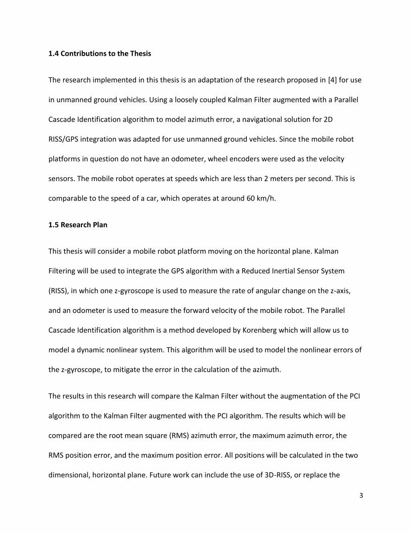
1.4 Contributions to the Thesis
The research implemented in this thesis is an adaptation of the research proposed in [4] for use
in unmanned ground vehicles. Using a loosely coupled Kalman Filter augmented with a Parallel
Cascade Identification algorithm to model azimuth error, a navigational solution for 2D
RISS/GPS integration was adapted for use unmanned ground vehicles. Since the mobile robot
platforms in question do not have an odometer, wheel encoders were used as the velocity
sensors. The mobile robot operates at speeds which are less than 2 meters per second. This is
comparable to the speed of a car, which operates at around 60 km/h.
1.5 Research Plan
This thesis will consider a mobile robot platform moving on the horizontal plane. Kalman
Filtering will be used to integrate the GPS algorithm with a Reduced Inertial Sensor System
(RISS), in which one z-gyroscope is used to measure the rate of angular change on the z-axis,
and an odometer is used to measure the forward velocity of the mobile robot. The Parallel
Cascade Identification algorithm is a method developed by Korenberg which will allow us to
model a dynamic nonlinear system. This algorithm will be used to model the nonlinear errors of
the z-gyroscope, to mitigate the error in the calculation of the azimuth.
The results in this research will compare the Kalman Filter without the augmentation of the PCI
algorithm to the Kalman Filter augmented with the PCI algorithm. The results which will be
compared are the root mean square (RMS) azimuth error, the maximum azimuth error, the
RMS position error, and the maximum position error. All positions will be calculated in the two
dimensional, horizontal plane. Future work can include the use of 3D-RISS, or replace the
4
Kalman Filter with a Particle Filter, which does not require linearization of errors during its
estimation process.
1.6 Thesis Outline
The thesis is structure as follows:
Chapter 1 gives a brief introduction to the mobile robot platform, the problem statement, and
the scope of research for this thesis.
Chapter 2 contains a brief background about GPS navigation, an introduction to the frames of
reference, background in dead reckoning, and a literature review about land vehicle navigation,
as well as unmanned ground vehicle navigation. It provides methods of integration of GPS and
Inertial Navigation Systems (INS), as well as methods to reduce the IMU errors.
Chapter 3 provides a detailed look into the Parallel Cascade Identification algorithm. Section
3.1 Introduces the PCI algorithm, and Section 3.2 provides an overview of the PCI algorithm.
Section 3.3 provides the equations used when calculating the linear response of the dynamic
linear system, and Section 3.4 provides equations used during the modeling of the static
nonlinear system. Section 3.5 introduces a criterion in adding a cascade to the PCI algorithm,
and Section 3.6 provides a list of stopping criteria for the PCI algorithm.
Chapter 4 provides the methodology used in this thesis. Section 4.1 provides the calculations
used for 2D/RISS. Section 4.2introduces loosely coupled filtering methods, and Section 4.3
provides an introduction to Kalman Filtering. Section 4.4 explains the augmentation of the PCI
algorithm with the Kalman Filter.
Chapter 5 is a look into the sensors used and their specifications, and the mobile robot. It also
features the connections used to connect these sensors to the host machine.

5
Chapter 6 is a discussion of the results of the KF augmented with the PCI, which is compared to
the KF without the PCI. Results compared are RMS azimuth error, the maximum azimuth error,
the RMS position error, and the maximum position error.
Chapter 7 is a conclusion of the work provided in this thesis, as well as recommendations for
future work.

6
Chapter2 - Background
2.1 Brief History of Navigation
Navigation is described as the skill or process of plotting a route and directing a vehicle, along
the route. Navigation comprises of various methods and technologies to determine the
position, speed, and orientation of the moving body via measurements [5].
The earliest forms of navigation involved traveling by ship near a coastline, and making note of
the coast to estimate the distance travelled. This later evolved into using the stars or midday
sun to measure latitude, and then using time and speed measurements to measure longitude.
Time was measured using a sand hourglass. Speed was measured by tossing a piece of wood
into the water, and counting the knots in the rope as it slipped through the navigator’s hands.
The amount of distance travelled would then be calculated using distance = speed x time. This
technique is known as dead reckoning [6].
2.2 GPS Positioning
The GPS comprises of over 24 satellites which revolve around the Earth in six orbits [7]. These
satellites measure the distance between the receiver and itself, and from the comparison of the
distances of multiple satellites, the position of the receiver can be determined.

7
Figure 2.1: Twenty-Four Satellites in six orbits around the Earth [8].
At minimum, four satellites are required to provide an accurate 3D calculation of the position of
the receiver. Each satellite rotates the Earth twice per day, and the life span of the satellites is
typically around 7.5 years [7, 8]. The GPS satellites transmit a signal of its measurements at
frequencies L1 and L2. L1 has a frequency of 1575.42 MHz, while L2 has a frequency of 1227.6
MHz [9, 10]. The signal sent by the satellite stores measurements such as: the pseudorange, the
Doppler velocity, the carrier phase, and the standard deviation of the measurements. Given this
information, the receiver can determine the position of the satellites, then the position of the
moving body [7, 10]. The receiver position can be determined via pseudorange, and the
receiver velocity can be determined via the Doppler measurements. [11]
The accuracy of the GPS signal is subject to many sources of error. These errors include: errors
originating at the satellite, errors originating during signal propagation, errors originating at the
receiver, and errors due to the overall geometry of the satellites overhead. [12]

8
2.2.1 Errors Originating at the Satellite
Errors which originate at the satellite consist of satellite clock errors and satellite orbital errors.
The satellite orbital error is the difference between the actual satellite position, and the
satellite position calculated by the receiver. The satellite clock error is the drift of the satellite
clock time from the GPS system time. These errors are predicted by control algorithms, and
then broadcasted to the satellites every half hour via ephemeris data [13].
2.2.2 Errors Due to Propagation
As the GPS signal passes through the ionospheric and tropospheric layers of the Earth’s
atmosphere, they time to reach the receiver is delayed. The delay in time ultimately results in
inaccuracies in the calculation of position and velocity. The ionosphere lies between 60 to 1000
kilometers above the surface of the Earth. The ionosphere consists of various ionized gasses
whose ionization level changes with solar activity. The troposphere is located 50 km above the
Earth’s surface, and mainly consists of dry gasses and water vapour. The troposphere is
refractive, which causes a decrease in the speed of propagation. [12]

9
Figure 2.2: Propagation delays due to Ionosphere and Troposphere. Adapted from [13].
2.2.3 Errors Originating at the Receiver
The main sources of error at the receiver are receiver clock error, and receiver noise. Due to the
inexpensiveness of receiver clocks when compared to satellite clocks, receiver clocks are much
less accurate. This error can be corrected by the navigation processor. The measurement noise
at the receiver is due to component nonlinearity, and thermal noise. This is usually modeled as
white noise, and cannot be avoided. [12]
Signal Delay
Ionosphere
60 to 1000km Troposphere
50 km

10
2.2.4 Geometry of Satellites
A higher angular separation between satellites represents good geometry between the
satellites. The higher the angular separation, the more precise the information provided to the
receiver is. The accuracy of the geometry between the satellites is represented by the
Geometric Dilution of Precision, or GDOP. A high value in GDOP represents poor geometry f the
satellites, thus resulting in higher error. Conversely, a low value in GDOP represents good
geometry, and results in smaller error. [13]
Figure 2.3: Desired and Undesired Satellite Geometry.
a) Good satellite geometry b) Bad satellite geometry
11
2.3 Reference Frames
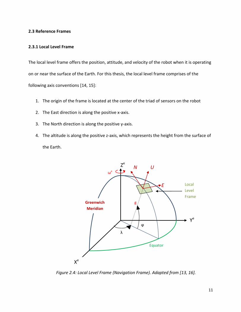
2.3.1 Local Level Frame
The local level frame offers the position, attitude, and velocity of the robot when it is operating
on or near the surface of the Earth. For this thesis, the local level frame comprises of the
following axis conventions [14, 15]:
1. The origin of the frame is located at the center of the triad of sensors on the robot
2. The East direction is along the positive x-axis.
3. The North direction is along the positive y-axis.
4. The altitude is along the positive z-axis, which represents the height from the surface of
the Earth.
Figure 2.4: Local Level Frame (Navigation Frame). Adapted from [13, 16].
ωe
λ
ϕ
Ze
N U
E
g
Equator
Greenwich
Meridian
Ye
Xe
Local
Level
Frame

12
2.3.2 Body Frame
The body frame is the frame of reference which moves along the axes of the accelerometers
and gyroscopes. The body frame is usually oriented such that [17]:
1. The origin of the frame is in center of gravity of the robot
2. The y-axis is the in the forward direction of the robot
3. The x-axis points towards the transverse direction.
4. The z-axis is in the vertical direction of the robot, completing the right hand rule. The z-
axis can point down or up, depending on the direction of the transverse axis. If it is
pointed upwards, the gravity component of the acceleration will be negative.
Figure 2.5: Body Frame, with vehicle at origin.
2.3.3 LLF to Body Frame Conversion
In order to convert from the body frame to the local level frame, one requires the pitch, roll,
and azimuth from the body frame. The azimuth is defined as the rotation about the z-axis from
Forward Direction, Yb
Transverse Direction, Xb
Vertical Direction, Zb

13
the North axis, and is denoted by A. The roll, denoted by Θ, is the rotation about the roll axis, or
the y-axis, from a desired orientation. The pitch, denoted by ρ, is the rotation about the pitch
axis, or the x-axis, from the desired horizontal plane. Through mechanization, one can obtain
the rotations in the pitch, azimuth, and roll. The transformation from the body frame to the
local level frame can be expressed via , the rotation matrix shown in 4.1 [14, 15]:
2.4 Dead Reckoning and Internal Navigation Systems
Dead reckoning is a method used in which the position of an object is calculated provided the
starting position is known, as well as previous displacements [18]. The minimum requirements
for a dead reckoning algorithm are speed indication, and direction indication. The distance the
vehicle travelled can be obtained via the average speed, multiplied by the time. The
displacement can be obtained by plotting the distance travelled along the measured direction
[17]. The position x at time n can be calculated using Equation 2.2:
Where di is the distance traveled, and Θi is the orientation of the object, which can be obtained
via:

14
Where ωi is the angular rate of change of the orientation of the vehicle. [18]
In Inertial Navigation Systems (INS), the most commonly used Internal Measurement Units
(IMU) are gyroscopes and accelerometers. Gyroscopes are bodies that display strong angular
momentum characteristics, and maintain a known spatial direction through control of torque.
The vehicular navigation, gyroscopes are often used to measure the orientation of the vehicle.
Accelerometers utilize Newton’s Second Law of Motion, which states that force is a product of
mass and acceleration. To obtain the position and velocity based on the measured acceleration,
the acceleration is integrated over time. The first integration of acceleration yields the velocity
of the vehicle, while a second integration yields the displacement [19]. Using the position,
velocity, and orientation of the vehicle, a vehicles position and velocity can be calculated at any
time using dead reckoning equations 2.2 and 2.3.
Gyroscope and accelerometer measurements are taken in the body frame, as shown in section
2.3.2. The gyroscopes measure the rotations around the respective axes, and the
accelerometers measure the accelerations on these axes. Using the rotation matrix in 2.3.3, the
measurements taken in the body frame can be converted to the LLF frame [17].
Most accelerometers and gyroscopes experience a multitude of error types. The main types of
error that these measurement devices undergo that will be discussed are: Bias offset and drift,
Scale Factor, axis misalignment, and noise. [13]

15
2.4.1 Bias Offset and Drift
The bias error consists of two parts. The offset, which is deterministic, refers to the offset in
measurement provided by the measurement sensors. This can easily be removed through
calibration. Typically, for gyroscopes and accelerometers, the offset is determined during the
stationary portion of the data. During this portion of data, the output of the sensors should be
centered about 0. To remove this, a mean of the stationary data is taken, and then this value is
subtracted from the entirety of the data. [16]
The bias drift is the stochastic part of the bias error. The bias drift is the variation of the
measurement due to temperature. The bias drift uncertainty is random in nature, and therefore
can only be modeled via stochastic processes [16]. Figure 2.1 shows the offset and drift in
typical sensor data.
Figure 2.6: Effect of Bias on sensor Output. Adapted from [13].
True Output

16
2.4.2 Scale Factor
The scale factor is the constant ratio between the actual sensor measurement and the output
signal. The scale factor is mostly affected by variations in temperature. Random changes in
scale factor are known as scale factor instability. Conversely, the capability for the sensor to
accurately measure the angular rate or acceleration is called scale factor stability. [16]
Figure 2.7: Effect of Scale Factor on Sensor Output. Adapted from [13].
2.4.3 Non-orthogonality of the IMU Axes
During the mounting of the sensors, it is possible that the one or more of the axes are not
orthogonal to the others. For example, the z-axis may not be 90 degrees from both the x and y
axes. If the IMU axes are not aligned properly, each axis will be affect by the measurements
along the other two axes. [15, 16]
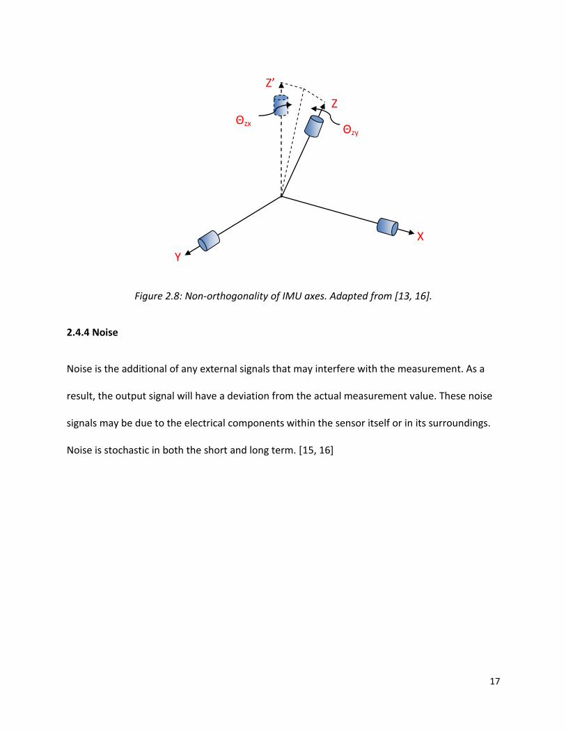
17
Figure 2.8: Non-orthogonality of IMU axes. Adapted from [13, 16].
2.4.4 Noise
Noise is the additional of any external signals that may interfere with the measurement. As a
result, the output signal will have a deviation from the actual measurement value. These noise
signals may be due to the electrical components within the sensor itself or in its surroundings.
Noise is stochastic in both the short and long term. [15, 16]
Θzx Θzy
X
Y
Z’
Z

18
Figure 2.9: Effect of Noise on Sensor Output. Adapted from [13].
2.5 Literature Review
Yoon et al. [20] implemented control algorithm for an automated ground vehicle to navigate
through waypoints using GPS as a coordinate system, and a compass to provide azimuth. These
waypoints were place along a predefined path the vehicle was to navigate. Using the compass
to define its current azimuth, the vehicle could redefine its direction to direct itself to the
desired waypoint. His tests had shown that turns with a larger radius resulted in a higher error.
However, in Yoon’s second experiment, it was found that the GPS signal was unstable and
provided poor accuracy. Yoon suggested to integrate and inertial navigation system to assist
the GPS during these unstable moments.
In [21], Sukkarieh et al combined the use of GPS and IMU to provide a navigation solution.
During his investigation, he determined the faults in IMU and GPS measurements. Sukkarieh
noted that at low frequency, the IMU faults were due to bias, which could be removed through
19
calibration. However, over time, bias drift was still a major factor in error. This drift could be
corrected with the GPS. However, the high frequency faults were located in the GPS, notably
due to multipath. These errors could be monitored and corrected by observing the GPS
covariances in the Kalman Filter. During his experiments, he noted that a correction in the IMU
error lead the automated vehicle to correct its heading, if it was facing the wrong direction.
Eric North developed a mobile robot with which Unmanned Ground Vehicle (UGV) data can be
gathered. This robot was built to be simple to fabricate, to be durable, modular, and easy to
maintain. In his work he also developed a predictive error model for use in a Kalman Filter to
estimate position, velocity, and attitude of a vehicle in both 2D and 3D navigation. [15]
Aono, using fiber optic gyroscopes, a kinetic GPS, and a roll pitch sensor, was able to provide a
positioning algorithm for automated lawn mowers. These mowers would travel in straight lines
with an arcing path. These sensors were fused using a Kalman Filter, and it was found that the
GPS error of 1 meter was reduced to 0.2 meters through sensor fusion [22].
In navigation, it is useful to have your current position and attitude provided to you in real time.
In [23], Walid AbdelFatah developed a low cost, real time embedded navigation system for
mobile robots. Using a MicroBlaze soft-core embedded processor, AbdelFatah developed a 2D
reduced inertial sensor system integrated with GPS via Kalman Filter which was able to provide
a real time navigation solution. [23]
In [24], Atia introduced WiFi and Reduced Inertial Sensor System (RISS) positioning for indoor
environments. Due to the low cost sensors used, and the extremely noisy WiFi signal strength
both having nonlinear errors, a mixture Particle Filter with adaptive weighting techniques was

20
used. The nonlinearity of the WiFi signal strength made Kalman Filter very difficult to use, thus
making the choice to use a particle filter clear. Atia was able to integrate WiFi positioning with
RISS sensors to smooth WiFi noisy position estimates, and reduce the sensor noise, which
ultimately lead to a respectable navigation solution. [24]
Chan suggested the use of magnetic markers for use as a position reference system for land
based vehicles. These magnets were placed in the road as reference points, and were sensed
via a magnetometer on the vehicle’s front end bumper. Through peak mapping, the vehicle was
able to maintain its trajectory along these magnet markers. It was noted that the Earth’s
magnetic field, as well as large objects show a considerable distortion on the readings from the
sensors. [25]
In land vehicle navigation, Zhi Shen was able to introduce a new nonlinear technique to
enhance the performance of low cost positioning for land based vehicles. Using the Fast
Orthogonal Search (FOS), Shen was able to model and handle the nonlinear errors of low cost
Internal Measurement Unit devices. The FOS algorithm was augmented with a Kalman Filter to
suppress both the linear and nonlinear error models of the measurement units. This KF/FOS
integration was then implemented in hardware using the TMS320DM642 digital signal
processing evaluation module, where the data could be logged and evaluated in real time. [26]
In [27], a Kalman Filter was augmented with an autoregressive (AR) model, as well as
neurofuzzy (NF) modules for nonlinear modeling to improve navigation in land based vehicles.
The Neurofuzzy model used an adaptive NF inference system P-δP model. The NF model was
trained during GPS availability to recognize patterns, and used this model during GPS outages to

21
predict the INS errors. When comparing the KF augmented with 1st order Gaussian model
(KFGM), the KF with the AR model (KFAR), and the KF with the ANFIS model (KFANFIS), it was
found that the KFAR model was superior to the KFGM model by 20%, and the KFANFIS model
lowered the error to by 64% in comparison to the KFAR model.
In [28], an open loop Kalman Filter was used to provide a 2D navigational solution for land
based vehicles. Iqbal et al. used a system dubbed multisensory system (MSS), which consisted
of one gyroscope and an odometer as the vehicle sensors, similar to RISS. Both the gyroscope
and odometer assumed first order Gaussian error models. The covariance matrices were then
tuned to optimize the KF calculations.
Georgy used a mixture particle filter in [29] to propose a 3D navigational solution using
RISS/GPS integration in land based vehicles. The RISS sensors included two accelerometers
whose measurements were used to calculate pitch and roll, the z-axis gyroscope, and an
odometer. Georgy found that the proposed particle filter 3D RISS/GPS integration performed
better than its Kalman filter counterpart, as well as its 2D particle filter predecessor. In [30],
Atia et al. expanded on this and used an Arm Cortex A8 processor to provide a real time
solution. Atia et al, implemented a technique called median-cut clustering to reduce the PF
iteration time without affecting the overall accuracy.
In [31], Georgy implemented the Parallel Cascade Identification (PCI) algorithm to model the
stochastic drift of a low cost gyroscope. This PCI algorithm was augmented to a loosely coupled
Mixture Particle Filter (MPF) to provide a 2D navigation solution using RISS/GPS integration in
land based vehicles. It was found that the MPF augmented with the PCI performed better than
22
both MPF which used a Gauss Markov model, as well as the MPF with a white Gaussian noise
model.
In [4], the PCI algorithm was used to model the azimuth error for 2D car navigation. This
algorithm was augmented to the Kalman Filter in a loosely coupled fashion. This 2D integration
used RISS/GPS integration, and it was found to have performed better than the KF without the
PCI augmented.
The research implemented in this thesis is an adaptation of the research proposed in [4] for use
in low mobility land vehicles. At low motilities, the lower speed of the robot results in lower
errors in the Kalman Filter and Kalman Filter with PCI outputs, as the azimuth error is
proportional to vehicle speed [32]. In [4], the outages had resulted in maximum position errors
in the hundreds of meters with the Kalman Filter. Since position is dependent on speed, a lower
speed will results in a lower displacement, which in turn would be less susceptible to error.
Using a loosely coupled Kalman Filter augmented with a Parallel Cascade Identification
algorithm to model azimuth error, a navigational solution for 2D RISS/GPS integration was
adapted for use unmanned ground vehicles. Since the mobile robot platforms in question do
not have an odometer, wheel encoders were used as the velocity sensors. The mobile robot
operates at speeds which are less than 2 meters per second. This is comparable to the speed of
a car, which operates at around 60 km/h.
23
Chapter 3 - Parallel Cascade Identification Algorithm
3.1 Introduction to the PCI Algorithm
The Parallel Cascade Identification (PCI) Algorithm was proposed by Korenberg in [33]. The PCI
algorithm was developed to approximate an unknown dynamic nonlinear system, given the
input and output are known. The PCI algorithm models the input/output behavior of a system
by summing the parallel cascades. Each cascade consists of a dynamic linear (L) and static
nonlinear (N) element.
Korenberg showed that any discrete-time Volterra series with finite memory and order can be
represented by a finite sum of parallel LN cascades, where the N elements are polynomials. This
technique does not depend on white Gaussian noise as input, but the L and N elements may
vary depending on the properties of the input chosen. [34]
The PCI algorithm finds LN cascades individually given a known input and a known output. The
first cascade uses the actual output to model the system in question. Each successive cascade is
obtained based on the residual, where the residual is the difference between the actual output
and the output of the cascades identified until then. Each additional cascade reduces the mean
squared error (MSE) of the output of the parallel cascade model from the actual output over
the training data. Cascades are added until one of the stopping criteria are met, one of which
includes the MSE reaching a threshold value. [32, 34]

24
3.2 Overview of the PCI Algorithm
The PCI algorithm models an unknown dynamic nonlinear system with parallel cascades of a
dynamic linear (L) element followed by a static nonlinear (N) element. Of the unknown system,
the input x(n) and the output y(n) are known (where n = 0,…,T). The length of the training data
is given by T. We assume that the output can depend on delayed input values x(n-j),for j = 0,…,R
(where R+1 is the modeled memory length of the system), and the maximum degree of
nonlinearity required for a good approximation of the system is D. [32, 34]
Korenberg developed several algorithms to build the parallel cascade. The version of the
algorithm used in this thesis is as described in [34]:
1. Approximate the dynamic nonlinear system by a first cascade of a dynamic linear (L)
element followed by a static nonlinear (N) element. The output of the first cascade is
z1(n).
2. Compute the first residual: y1(n)= y(n) – z1(n)
3. Approximate the new nonlinear system having input x(n) and output being the residual
of the previous cascade, y1(n), by a cascade L2 followed by N2. The output of this cascade
is z2(n).
4. Compute the second residual: y2(n)= y1(n) – z2(n).
5. And so on…
In each cascade, we must calculate the impulse response of the linear element, and apply the
fitting of the polynomial nonlinearity to the nonlinear element. We must also make sure the
cascade meets a certain condition before adding it to the model. Each after the addition of a

25
cascade, we check if it meets one of the stopping criteria to stop the PCI algorithm. The details
of each of these steps are detailed in the subsections below. [32, 34]
Figure 3.1: The idea of the PCI algorithm. Adapted from [35] and based on [33, 34].
3.3 Calculation of the Impulse Response of the Linear Element
When identifying the i-th cascade, the current residual before the addition of the i-th cascade is
yi-1(n). The output of the i-th cascade is denoted zi(n). To get the impulse response of Li at the
beginning of the i-th cascade, we use cross correlations of the input x(n) with the current
residual yi-1(n).
(a) Input residual cross correlation
Dynamic
Nonlinear
System
New
Nonlinear
System
L1 N1
L2 N2
x(n) x(n)
x(n) x(n)
y(n) z1(n)
z2(n) y1(n) = y(n)-z1(n)
a) Original unknown nonlinear system b) First LN cascade approximation
c) New Nonlinear system whose output is first residual
d) Second LN cascade

26
(b) , where the sign chosen is random, and A is chosen at random
from 0,…,R. The variable c is chosen such that c0 as
0, where the overbar
represents a finite time average from n = R to n = T as in .
(c)
(d) The expression can be used until:
However, the third order cross correlation is typically enough.
After calculating gi(j), the output ui(n) is calculated via convolution of the impulse response and
the input:
Before polynomial fitting, the following is usually done for computation purposes. First,
is calculated. Then gi(j) is adjusted to ensure
by: [35, 36]
3.4 Fitting the Polynomial Nonlinearity
To find the polynomial coefficients of the static nonlinearities, best fitting of the current
residual can be used. The D+1 coefficients aid, of the Ni which follows Li that best fit to minimize
the MSE, are found as follows:

27
This leads to D+1 equations with D+1 unknowns “aid”
These D+1 linear equations with D+1 unknowns are solved to get the polynomial coefficients of
the nonlinear element of the cascade. [35]
3.5 Condition for Adding a New Cascade to the Model
Before adding the i-th cascade whose output is zi(n)to the model, it must satisfy the condition:
If the cascade does not fulfill the condition, the cascade is discarded and a new candidate
cascade is built. The cascade helps to choose unnecessary cascades, which are simply modeling
noise. [32,34]
3.6 Stopping Condition of the PCI Algorithm
The process of building a parallel cascade can end if it fulfills any one of these stopping
conditions: [32, 34]
1. When a certain number of cascades is added
2. When a certain number of cascades is tested (whether or not they have been added)

28
3. When the MSE is sufficiently small
4. When no remaining candidate cascade can reduce the MSE more than a small threshold
level.
If any of these conditions are met, the PCI algorithm is halted and no additional cascades
are added to the model.
29
Chapter 4 - Methodology
4.1 2D RISS – Advantages Over Full IMU
In 2D Reduced Inertial Sensor Systems (RISS), the z-axis gyroscope is used to measure the
azimuth, and the wheel encoders of the robot are used to measure the velocity. This is a much
smaller system than the full IMU positioning, which features three accelerometers and three
gyroscopes. Due to the reduction of the sensors from six to three, a reduction in the overall
cost of the system is also implied.
For 2D RISS in land vehicles, one can assume that the only direction of movement is in the
direction that the land vehicle is facing. This means that the vehicle does not move along the x
or z axes. This is due to the assumption that the vehicle is on the horizontal plane, and due to
the non-holomic restraints of the vehicle. Furthermore, the pitch and roll of the vehicle are
assumed constant, as the vehicle only moves on the horizontal plane. [35]
In order to calculate the azimuth, one must first calculate the rate of change of the azimuth.
Using the gyroscope readings, as well as the wheel encoder readings, the yaw can be calculated
using Ve, the latitude, Φ, and the nominal radius of the Earth, RN. The yaw must also be
compensated with the component of the earth’s rotation, and the rotation of the local level
frame on the earth’s curvature. Using the above variables, the rate of change of the azimuth
can be calculated as:

30
Where ωz is the measurement made by the z-axis accelerometer, ωe is the Earth’s rotation rate,
φ is the latitude of the robot, Ve is the Eastern velocity of the robot, RN is the normal radius of
the Earth, and h is the altitude of the robot. The azimuth is obtained by integrating the rate of
change of the azimuth.[13]
From the wheel encoders, the translational velocity, Vtrans, and the rotational velocity, Vrot, are
extracted. These must be converted into the east and north directions, using the azimuth
previously calculated. [23]
Where Vtrans is the translational velocity of the robot, or the forward moving velocity; and A is
the azimuth of the robot. From the velocity, the rate of change of latitude and longitude can be
calculated by integration. The rates of change in the position are integrated, and then added to
the previous iterations latitude and longitude, to get the current position.
Where RM is the meridian radius of the earth, RN is the normal radius of the Earth, is the rate
of change in latitude, and is the rate of change in longitude. [23]
4.2 Loosely Coupled GPS/INS integration
In a loosely coupled GPS/INS integration, both GPS and INS systems operate separately, and
provide separate navigation solutions. One solution is provided from INS or RISS, and one

31
solution is provided from the GPS position. The solutions for both GPS and INS are usually fed
through an integration algorithm to model the error of the INS component. During GPS
outages, the integration uses the developed error model to estimate the INS error. Using this
estimated error, the solution can be calculated by subtracting the error from the INS solution.
[13]
Figure 4.1: Block Diagram for Loosely Coupled Algorithm.
The main advantage of the loosely-coupled model is its simplicity and redundancy. Since it uses
the final solution for both the GPS and INS algorithms, it can be used with any INS and GPS
equipment. The main disadvantages of the loosely coupled integration are the uncompromised
measurement noise, and satellite reliability. Since the loosely coupled integration assumed the
noise has been compensated, when there is measurement noise the integration solution is
-
-
+
+ Sensor
Measurements
GPS Navigational Solution
Integrated Navigational
Solution
INS Navigational Solution
GPS
Receiver
Mechanization
Integration
32
negatively impacted. Since one of inputs of the integration comprises the GPS position and
velocity solution, a minimum of four satellites is required in order to update the integration
method. [13]
4.3 Kalman Filtering
The integration filter used in this work is the Loosely-Coupled Kalman Filter. The Kalman Filter
was developed in November of 1958 by Rudolf Emil Kalman, who applied a notion of state
variables to the Wiener Filter. It is an estimator which is used to predict the instantaneous state
of a linear dynamic system, which is polluted with uncorrelated (white) noise. The Kalman Filter
utilizes the probability distributions of the state variables to provide statistical characterization
of the estimation problem. The Kalman Filter is uses a model of estimation that distinguishes
between phenomena (observables), noumena (known state), and knowledge about the
noumena that can be deduced from the phenomena [37].
While the GPS signal is available, the Kalman filter develops an error model based on the GPS
position and velocity, and the RISS/INS solution. During GPS outages, or when the number of
visible satellites is less than four, the integration uses the error model obtained via the Kalman
filter to estimate the position, velocity, and orientation of the mobile robot [13]. These error
models are required, as the nonlinear errors of the accelerometer and gyroscope sensors lead
to the calculated position, velocity, and attitude of the vehicle to drift as time progresses.
Using covariance matrices R (measurement noise), Q (system noise), and P (error state vector),
as well as the system & measurement models (x and z), and the state transition and design
matrices (F and H), the Kalman Filter can predict error states. [38]

33
First, the error states and covariance matrices are initialized. The next state (a priori) is
predicted using the previous iteration and the state transition matrix. Then, the error
covariance is predicted. This prediction is used with design matrix H, and covariance matrix R to
calculate Kalman gain. Using the Kalman gain, the a posteriori (updated) state estimate is
calculated. The error covariance is then updated for use in the following iteration [38]. This
process is shown in Figure 4.2.
4.3.1 System Model
The errors produced by the sensors are nonlinear and dynamic, so they are described by
differential equations. In the Kalman Filter, these nonlinear systems are linearized to obtain a
set of linear differential equations to define the error states. The error state vector in a 2D RISS
system is represented by:
A priory
Information
Initial
Conditions
Zk
Error state prediction
Error covariance
prediction
Kalman Gain
Update state estimate
Update error
covariance
Figure 4.2: Block Diagram for Kalman Filter Process.
Initialization

34
The rate of change of the RISS position errors are represented by:
Where is the error in the rate of change in latitude, is the error in the rate of change in
longitude, is the rate of change in the eastern velocity, and is the rate of change
in the northern velocity. [23]
The rate of change of the RISS velocity error is represented by:
Where aforward is the acceleration derived from the wheel encoders, δaforward is the error in the
forward wheel encoder derived acceleration, is the error in the rate of change of the
eastward velocity, and is the error in the rate of change of the northward velocity.
The rate of change in the azimuth error is defined simply by:
Where is the error in the rate of change in the azimuth, and is the error in the
gyroscope measurement. [23]
35
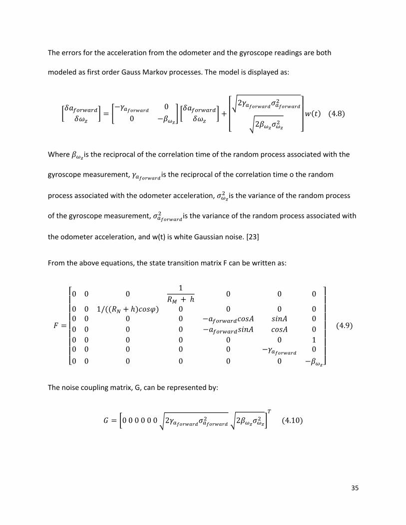
The errors for the acceleration from the odometer and the gyroscope readings are both
modeled as first order Gauss Markov processes. The model is displayed as:
Where is the reciprocal of the correlation time of the random process associated with the
gyroscope measurement, is the reciprocal of the correlation time o the random
process associated with the odometer acceleration, is the variance of the random process
of the gyroscope measurement, is the variance of the random process associated with
the odometer acceleration, and w(t) is white Gaussian noise. [23]
From the above equations, the state transition matrix F can be written as:
The noise coupling matrix, G, can be represented by:

36
4.3.2 Measurement Model
The measurement model of the RISS/GPS system can be represented as follows:
The design matrix, H, of the measurement model can be represented by [23]:
4.4 Kalman Filtering Augmented with PCI
When augmented with the Kalman Filter, the role of the PCI algorithm is to model the residual
azimuth errors which are not modeled by the KF. While the KF models the linear portion of the
errors, the PCI algorithm will model the nonlinear errors, as well as correct any errors due to
mis-modeling by the KF [4].
When the GPS signals are available, the KF normally outputs the outcome of the update phase.
For PCI modeling, the KF will also output the outcome of the prediction phase. The PCI
algorithm will then use this as its input to build its model on the azimuth error, in parallel to the
KF. The target output of the model consists of all the residual errors which were not modeled
by the KF. The azimuth derived from mechanization (Amech), the azimuth derived from GPS
(AGPS), and the predicted azimuth errors from the KF (δ-KF) are used to derive the residual
37
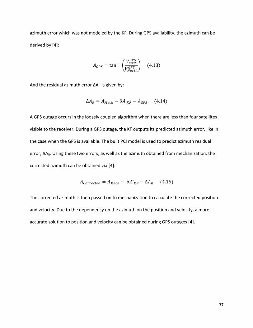
azimuth error which was not modeled by the KF. During GPS availability, the azimuth can be
derived by [4]:
And the residual azimuth error ΔAR is given by:
A GPS outage occurs in the loosely coupled algorithm when there are less than four satellites
visible to the receiver. During a GPS outage, the KF outputs its predicted azimuth error, like in
the case when the GPS is available. The built PCI model is used to predict azimuth residual
error, ΔAR. Using these two errors, as well as the azimuth obtained from mechanization, the
corrected azimuth can be obtained via [4]:
The corrected azimuth is then passed on to mechanization to calculate the corrected position
and velocity. Due to the dependency on the azimuth on the position and velocity, a more
accurate solution to position and velocity can be obtained during GPS outages [4].

38
4.5 Why Use Parallel Cascade Identification
As stated in Section 4.3, the Kalman Filter uses assumes linear transitions between the states.
However, low cost sensors are prone to nonlinear errors which are not accounted for in the
Kalman Filter. Because of this, the output of the Kalman Filter will include a residual nonlinear
error. The PCI will enable modeling of the nonlinear error during the GPS availability. During a
GPS outage, the modelled nonlinear error will be used to further correct the azimuth error,
after the linear corrections modelled by the Kalman Filter.
In mobile robots, accurate positioning information is required so the robots can perform its
given tasks. For example, one of the applications of mobile robots is mine detection. This type
of work requires pinpoint accuracy, as a small error can result in the loss of life or equipment.
Another example where this is required is in search and rescue, where exits, entrances, and
locations of threats are crucial information to the rescuers.

39
Chapter 5 - Experimental Setup
5.1 Overview
This chapter introduces the Mobile Robot Platform used and the sensor specifications of those
used. The sensors used are the Crossbow (Xbow) IMU, the NovaTel OEM-4 GPS receiver, the
Honeywell HG1700 IMU, U-blox GPS receiver, and VTI Gyroscopes and Accelerometers. For five
of the trajectories, the NovaTel SPAN unit was used as a reference, which used the OEM-4 GPS
receiver and the Honeywell IMU. The sixth trajectory used the T-PN data logger solution as a
reference.
5.2 Robot Platform
The mobile robot platform used was built by Eric North. It features one motor for each of the
two powered wheels, with wheel encoders on each motor. The wheel encoders are used to
count the number of pulses per second as the wheel turns. Using the pulses per second, one
can determine the speed of the vehicle. The speed data from the encoders is exported via an
RS-232 cable to the host machine. Each of the wheels of the robot is controlled individually
through the analog control box which is connected to the Sabertooth motor controller [15].
The motors are powered by two 12 volt DC batteries. A second set of 12 volt DC batteries are
used as a power supply for the sensors that are to be connected to the robot. The batteries will
power the robot for 1 to 1.5 hours, and the batteries for the motors can be replaced without
disrupting the power supply to the sensors [15].
40
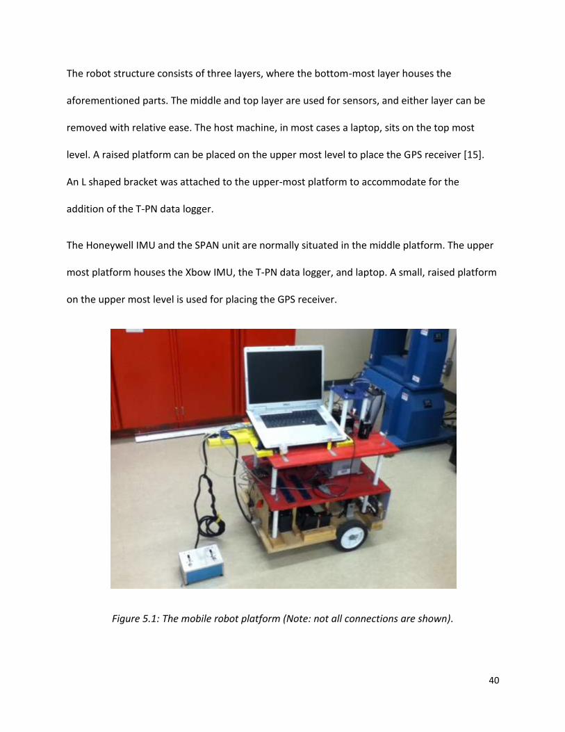
The robot structure consists of three layers, where the bottom-most layer houses the
aforementioned parts. The middle and top layer are used for sensors, and either layer can be
removed with relative ease. The host machine, in most cases a laptop, sits on the top most
level. A raised platform can be placed on the upper most level to place the GPS receiver [15].
An L shaped bracket was attached to the upper-most platform to accommodate for the
addition of the T-PN data logger.
The Honeywell IMU and the SPAN unit are normally situated in the middle platform. The upper
most platform houses the Xbow IMU, the T-PN data logger, and laptop. A small, raised platform
on the upper most level is used for placing the GPS receiver.
Figure 5.1: The mobile robot platform (Note: not all connections are shown).

41
The host machine or the laptop is connected to all of the sensors. The SPAN unit is connected to
the host machine via serial port, or a serial to USB converter. The T-PN unit is connected to the
host machine via serial-422 to USB. If the T-PN unit is not connected to the host machine, it is
able to log the data on a mini-SD card. The Xbow unit is connected to the host machine via
serial port, or serial to USB. Finally, the wheel encoder data is sent via serial to USB to the host
machine. The host machine runs a MATLAB script which sends a command to retrieve data
from the encoders at approximately 1Hz. The host machine collects the data from all these
sensors simultaneously.
Figure 5.2: Block Diagram of connections.
Wheel Encoders
SPAN Unit with OEM-4
GPS and HG1700
Xbow IMU
TP-N Data logger
TP-N Power Supply
u-Blox GPS Antenna
Serial 232 to
USB Serial 422 to
USB
Host
Machine

42
5.3 Sensors
5.3.1 Crossbow IMU300CC
The XBow IMU300CC is a six degree of freedom (6DOF) inertial measurement system used to
measure rotation rate and linear acceleration of a moving body. MEMS technology is used to
measure the accelerations and rotation rates of a moving body. The MEMS gyroscopes measure
the angular rates via the Corolis force in micro-machined vibratory MEMS sensors. The MEMS
accelerometers use differential capacitance to sense acceleration [39].
Figure 5.3: Xbow IMU300CC used in this thesis.
For the trajectories taken, the IMU was conFigured to run in continuous mode, sending
measurements via RS-232 cable at a rate of 100 samples per second. The measurement mode
43
was set to scaled sensor mode, rather than voltage mode [39]. Table 5.1 lists the specifications
for the Xbow IMU.
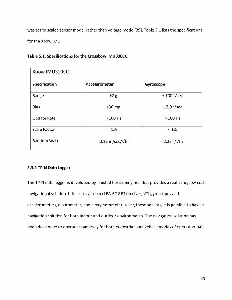
Table 5.1: Specifications for the Crossbow IMU300CC.
Xbow IMU300CC
Specification Accelerometer Gyroscope
Range ±2 g ± 100 ⁰/sec
Bias ±30 mg ± 2.0 ⁰/sec
Update Rate > 100 Hz > 100 Hz
Scale Factor <1% < 1%
Random Walk <0.15 m/sec/ <2.25 ⁰/
5.3.2 TP-N Data Logger
The TP-N data logger is developed by Trusted Positioning Inc. that provides a real-time, low cost
navigational solution. It features a u-blox LEA-6T GPS receiver, VTI gyroscopes and
accelerometers, a barometer, and a magnetometer. Using these sensors, it is possible to have a
navigation solution for both indoor and outdoor environments. The navigation solution has
been developed to operate seamlessly for both pedestrian and vehicle modes of operation [40].
44
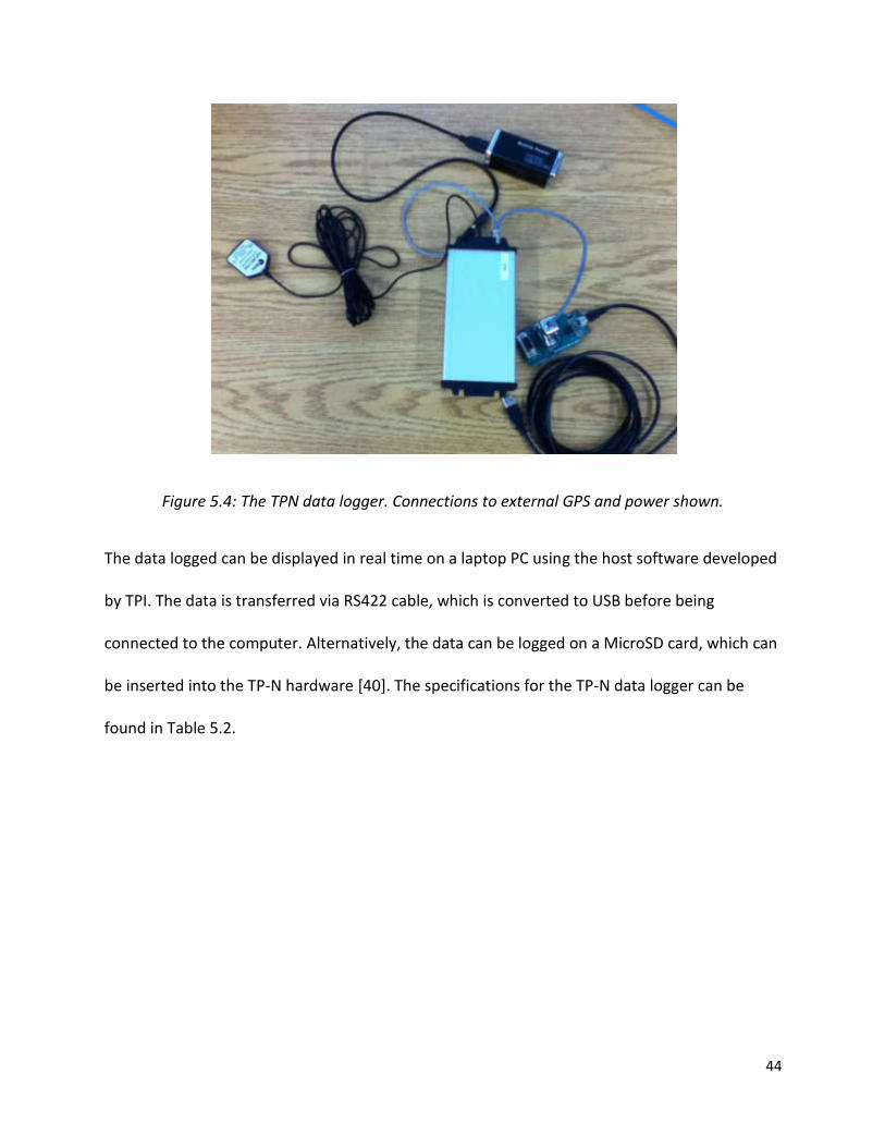
Figure 5.4: The TPN data logger. Connections to external GPS and power shown.
The data logged can be displayed in real time on a laptop PC using the host software developed
by TPI. The data is transferred via RS422 cable, which is converted to USB before being
connected to the computer. Alternatively, the data can be logged on a MicroSD card, which can
be inserted into the TP-N hardware [40]. The specifications for the TP-N data logger can be
found in Table 5.2.

45
Table 5.2: Specifications for the TP-N Data Logger
TP-N Data Logger
Specification VTI Accelerometer VTI Gyroscope
Range 2 g ± 100 ⁰/sec
Bias 16 mg ± 1.0 ⁰/hr
Scale Factor 2500 ppm 2000 ppm
Random walk 0.1 m/sec/ 0.45 ⁰/
Specification U-Blox LEA-6T GPS Receiver
Time to First Fix : Cold Start 65 sec
Time to First Fix : Hot Start 35 sec
Horizontal Position Accuracy: Single Point
L1
1.5 m
Horizontal Position Accuracy: SBAS 0.7m
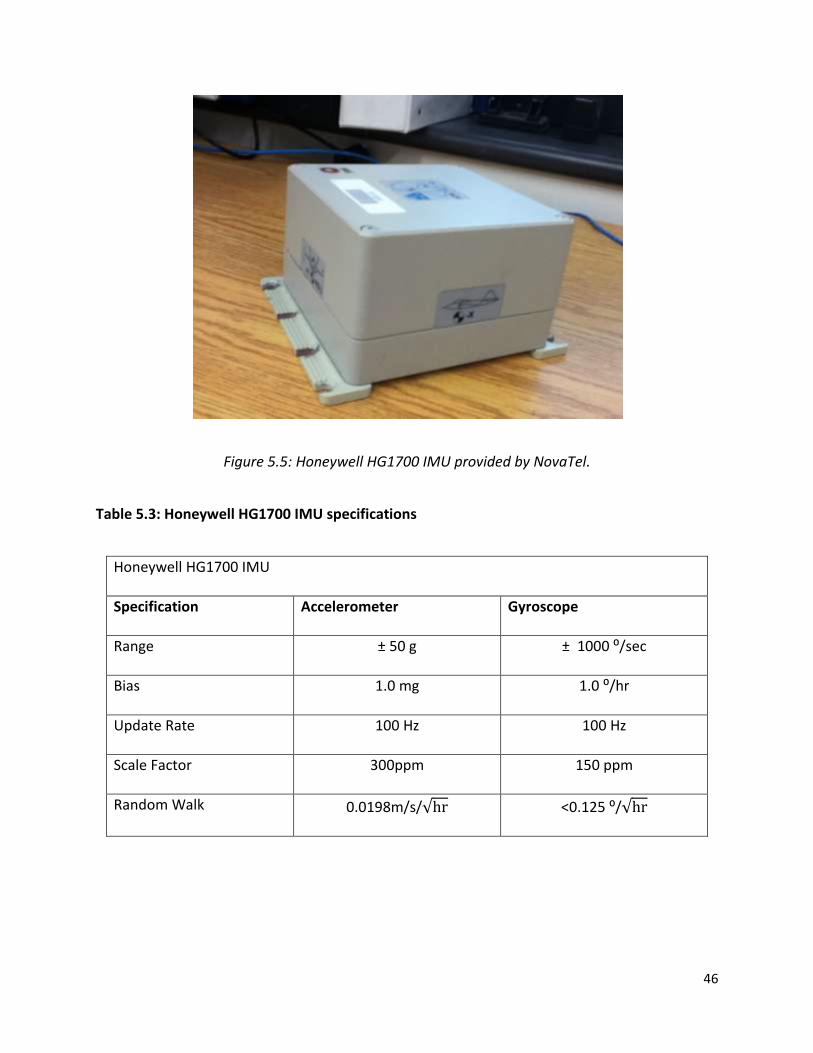
5.3.3 Honeywell HG1700 IMU
The Honeywell HG1700 is a tactical grade IMU which is a component used as reference during
the trajectories. The HG1700 uses three Ring Laser Gyroscopes (RLG) and three quartz
resonating beam accelerometers (RBA) for measuring rotation rate and linear acceleration. It
uses an external environmental ring isolator to filter common sources of unwanted noise. Table
5.3 details the specifications for the HG1700 IMU [41].
46
Figure 5.5: Honeywell HG1700 IMU provided by NovaTel.
Table 5.3: Honeywell HG1700 IMU specifications
Honeywell HG1700 IMU
Specification Accelerometer Gyroscope
Range ± 50 g ± 1000 ⁰/sec
Bias 1.0 mg 1.0 ⁰/hr
Update Rate 100 Hz 100 Hz
Scale Factor 300ppm 150 ppm
Random Walk 0.0198m/s/ <0.125 ⁰/

47
5.3.4 Novatel SPAN Unit
The NovAtel ProPak-G2 combines the Honeywell HG1700 IMU with the high accuracy NovaTel
OEM-4 GPS receiver via SPAN technology to formulate a high end solution. The SPAN
technology integrates raw inertial measurements with GPS information and raw GPS
measurements to formulate the navigation solution. When the number of GPS satellites visible
to the receiver is less than four, the SPAN unit is still able to produce an integrated solution via
raw measurements such as pseudorange. The high end solution provided by the ProPak-G2
SPAN unit is what was used as a reference during the majority of trajectories taken. The
specifications for the OEM-4 GPS receiver, which is used by the SPAN unit, are detailed in Table
5.4. [42]
Figure 5.6: NovaTel Span Unit, shown with OEM-4 GPS receiver and Honeywell HG1700 IMU.
48
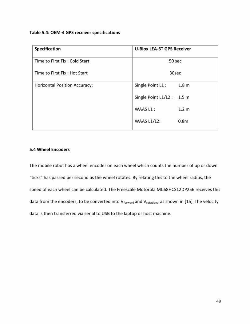
Table 5.4: OEM-4 GPS receiver specifications
Specification U-Blox LEA-6T GPS Receiver
Time to First Fix : Cold Start
Time to First Fix : Hot Start
50 sec
30sec
Horizontal Position Accuracy: Single Point L1 : 1.8 m
Single Point L1/L2 : 1.5 m
WAAS L1 : 1.2 m
WAAS L1/L2: 0.8m
5.4 Wheel Encoders
The mobile robot has a wheel encoder on each wheel which counts the number of up or down
“ticks” has passed per second as the wheel rotates. By relating this to the wheel radius, the
speed of each wheel can be calculated. The Freescale Motorola MC68HCS12DP256 receives this
data from the encoders, to be converted into Vforward and Vrotational as shown in [15]. The velocity
data is then transferred via serial to USB to the laptop or host machine.

49
Chapter 6 - Experiments and Results
Trajectories 1 through 5 were conducted during the summer season of 2010. These trajectories
were performed by Walid Abdelfatah [23]. The raw data for these trajectories were provided
for post processing. The details of Trajectory 6th, conducted in late 2012, are provided after the
discussion of the aforementioned trajectories. All of the data processing was done in MATLAB.
In all experiments, the memory length was 15, and the degree of nonlinearity was 2. Any
increases in either of these variables did not provide any further reduction in the MSE. To
restate the assumptions made in the post processing of the 2D-RISS experiments, we assume
that the vehicle is always on the horizontal plane, so pitch and roll are constant. We also
assume the vehicle can only move in the direction it is facing, due to its non-holomic
constraints. This means there is no movement in the x or z direction. Since MEMS sensors’
outputs may vary during different weather conditions due to temperature dependence, if these
experiments were done in the winter, the results may vary.
6.1 Trajectory 1
Trajectory 1 was performed in the parking lot at the Royal Military College of Canada with the
mobile robot. The duration of this trajectory was 11 minutes and 26 seconds. Two 60 second,
simulated outages were introduced to the open sky trajectory. The maximum speed of the
robot in this trajectory was 0.924 m/s, and the vehicle was always in motion. Figure 6.1 displays

50
Trajectory 1, with the outages circles in red. For Trajectory 1, MATLAB processed 685 seconds
worth of data in 10.73 seconds.
Figure 6.1: Trajectory 1, performed in open sky environment with two simulated outages.
The PCI algorithm was able to model the nonlinear azimuth error, by using the mechanization
azimuth, GPS azimuth, and KF azimuth error as inputs. The performance of the KF was
compared to the performance of the KF PCI algorithm in each of the outage scenarios. Both of
these algorithms use the NovaTel SPAN unit output as a reference. Each outage was placed
after a dramatic change in the robot’s orientation, to encompass large changes in the robot’s
sensors.

51
A zoomed in image of the first outage is shown in Figure 6.2. This outage takes place after a
right turn, as well as during a small, natural GPS outage. The outage can be noted in the GPS
path by the deviance from the straight line that the robot is heading.
Figure 6.2: A zoomed in image of the first simulated outage.
A zoomed in image of the second outage is shown in Figure 6.3. This outage takes place during
a left turn, near the end of the trajectory. Comparisons of the performance of the Kalman Filter
versus the KF Augmented with PCI for azimuth error can be investigated through these
simulated outages.

52
Figure 6.3: A zoomed in image of the second simulated outage.
The performance of the KF, versus the KF augmented with the PCI can be noted through the
errors in the RMS and max azimuth error, as well as the RMS and max position error. Figure 6.4
shows a bar graph comparing the RMS azimuth error. The RMS azimuth errors for the KFPCI
algorithm are 0.8818 degrees and 5.4813 degrees for first and second outages, respectively. In
contrast, the RMS azimuth error was 5.0072 degrees and 8.7919 degrees for the KF in the
respective outages. The KFPCI shows an improvement of 82.4 % in the first outage, and 37.7%
in the second outage.

53
Figure 6.4: RMS Azimuth Error for each outage Trajectory 1.
The bar graph displayed in Figure 6.5 displays the maximum azimuth error for each of the
outages. The maximum errors in the azimuth for the KFPCI algorithm are 1.499 degrees and
16.5188 degrees for the first and second outage, respectively. The KF algorithm shows a
maximum error of 5.3243 degrees and 21.4722 degrees for each respective outage. The KFPCI
shows an improvement in the error by 71.8% in the first outage and 23.1% in the second
outage.
0
1
2
3
4
5
6
7
8
9
10
1 2
Azi
mu
th E
rro
r in
De
gre
es
Outage Number
RMS Azimuth Error
KF RMS Azimuth Error
KFPCI RMS Azimuth Error

54
Figure 6.5: Maximum Azimuth Error for each outage in Trajectory 1.
The improvements in error will result in an improvement in the calculated position, as the
calculation of the position in the following iteration is dependent on the heading. The RMS
position error for each outage is depicted in Figure 6.6. The KFPCI RMS position error is 0.4593
meters, and 1.767 meters for the first and second outage, respectively. Conversely, the KF
shows RMS errors of 0.765 meters and 1.9436 meters for each of the respective outages. The
KFPCI shows an improvement in the RMS error of 40% in the first outage, and 9.1% in the
second outage.
0
5
10
15
20
25
1 2
Azi
mu
th E
rro
r in
De
gre
es
Outage Number
Max Azimuth Error
KF Max Azimuth Error
KFPCI Max Azimuth Error

55
Figure 6.6: RMS Position Error for each of the outages in Trajectory 1.
The maximum position error for each outage is depicted in the bar graph in Figure 6.7. The
KFPCI maximum position error is 0.8179 meters for the first outage, and 2.3684 second outage.
The KF shows maximum errors of 1.8251 meters and 2.8761 meters for each of the respective
outages. The KFPCI algorithm shows an improvement in the maximum position error of 55.2%
in the first outage, and 17.6% in the second outage.
0
0.5
1
1.5
2
2.5
1 2
Po
siti
on
Err
or
in m
ete
rs
Outage Number
RMS Position Error
KF RMS Position Error
KFPCI RMS Position Error

56
Figure 6.7: Maximum Errors in position for each outage in Trajectory 1.
6.2 Trajectory 2
Trajectory 2 also took place in the RMC parking lot with the mobile robot. The duration of the
trajectory was 11 minutes and 56 seconds. The trajectory was subject to three simulated
outages, as it was taken in an open sky environment. The maximum speed of the robot in this
trajectory was 0.9781 m/s, and the vehicle was always in motion. Figure 6.8 depicts the path
taken, and identifies each of the outages in red circles. For Trajectory , it took 15.59 seconds to
process 715 seconds worth of data in MATLAB.
0
0.5
1
1.5
2
2.5
3
3.5
1 2
Po
siti
on
Err
or
in m
ete
rs
Outage Number
Max Position Error
KF Max Position Error
KFPCI Max Position Error

57
Figure 6.8: Trajectory 2, performed in open sky environment with three simulated outages.
The PCI algorithm was able to model the nonlinear azimuth error, by using azimuth obtained via
mechanization, azimuth obtained by the GPS, and azimuth error obtained by the KF as inputs.
The performance of the KF was compared to the performance of the KF PCI algorithm in each of
the outage scenarios. Both of these algorithms use the Novatel SPAN unit output as a
reference. Each outage was placed after, or during a dramatic change in the robot’s orientation,
to encompass large changes in the robot’s sensors.
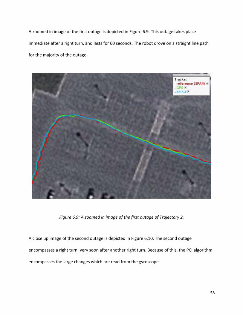
58
A zoomed in image of the first outage is depicted in Figure 6.9. This outage takes place
immediate after a right turn, and lasts for 60 seconds. The robot drove on a straight line path
for the majority of the outage.
Figure 6.9: A zoomed in image of the first outage of Trajectory 2.
A close up image of the second outage is depicted in Figure 6.10. The second outage
encompasses a right turn, very soon after another right turn. Because of this, the PCI algorithm
encompasses the large changes which are read from the gyroscope.

59
Figure 6.10: A zoomed in image of the second outage of Trajectory 2.
The final outage encompasses a gradual right turn, which occurs some time after the previous
one. Figure 6.11 shows the third outage, as well as 20 seconds before and 20 seconds after the
outage. The trajectory is isolated to remove confusion, as this part of the trajectory intersects
with a pervious portion.

60
Figure 6.11: A zoomed in image of the third outage isolated from Trajectory 2.
The performance of the KF, versus the KF augmented with the PCI can be noted through the
errors in the RMS and max azimuth error, as well as the RMS and max position error. Figure
6.12 displays a bar graph comparing the RMS azimuth error. The RMS azimuth errors for the
KFPCI algorithm are 0.4227 degrees, 1.074 degrees, and 6.7885 degrees for first, second, and
third outages respectively. In contrast, the RMS azimuth errors were 2.3492 degrees, 2.2292
degrees, and 12.1483 degrees for the KF in the respective outages. The KFPCI shows an

61
improvement of 42.2% in the first outage, 22.1% in the second outage, and 62.3% in the third
outage.
Figure 6.12: RMS Azimuth Error during each outage in Trajectory 2.
The bar graph displayed in Figure 6.13 displays the maximum azimuth error in each outage. The
first outage had a maximum error of 1.234 degrees for KFPCI and 2.5192 degrees for the KF.
The KFPCI showed an improvement of 51% over the KF in the first outage. The second outage
had a maximum azimuth error of 1.7546 for the KFPCI and 3.0052 for the KF. The second
outage showed an improvement in the azimuth of 41.6%, when comparing the KFPCI to the KF.
The third outage had maximum errors of 14.671, and 21.5814, for the KFPCI and KF algorithms
respectively. This KFPCI in this outage showed an improvement of 32% over the KF.
0
2
4
6
8
10
12
14
1 2 3
Azi
mu
th E
rro
r in
de
gre
es
Outage number
RMS Azimuth Error
KF RMS Azimuth Error
KFPCI RMS Azimuth Error
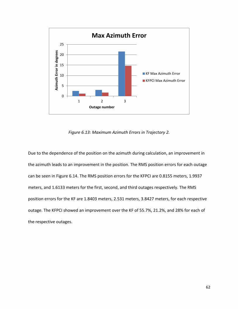
62
Figure 6.13: Maximum Azimuth Errors in Trajectory 2.
Due to the dependence of the position on the azimuth during calculation, an improvement in
the azimuth leads to an improvement in the position. The RMS position errors for each outage
can be seen in Figure 6.14. The RMS position errors for the KFPCI are 0.8155 meters, 1.9937
meters, and 1.6133 meters for the first, second, and third outages respectively. The RMS
position errors for the KF are 1.8403 meters, 2.531 meters, 3.8427 meters, for each respective
outage. The KFPCI showed an improvement over the KF of 55.7%, 21.2%, and 28% for each of
the respective outages.
0
5
10
15
20
25
1 2 3
Azi
mu
th E
rro
r in
de
gre
es
Outage number
Max Azimuth Error
KF Max Azimuth Error
KFPCI Max Azimuth Error

63
Figure 6.14: RMS Position Error for Trajectory 2.
The bar graph displayed in Figure 6.15 displays the maximum position error in each outage. The
first outage had a maximum error of 1.957 meters for KFPCI and 3.3864 meters for the KF. The
KFPCI showed an improvement of 42.2% over the KF in the first outage. The second outage had
a maximum position error of 2.8981 meters for the KFPCI and 3.7222 for the KF. The second
outage showed an improvement in the position of 22.1%, when comparing the KFPCI to the KF.
The third outage had maximum errors of 2.8252, and 7.484, for the KFPCI and KF algorithms
respectively. This KFPCI in this outage showed an improvement of 62.3% over the KF.
0
0.5
1
1.5
2
2.5
3
3.5
4
4.5
1 2 3
Po
siti
on
Err
or
in M
ete
rs
Outage number
RMS Position Error
KF RMS Position Error
KFPCI RMS Position Error

64
Figure 6.15: Maximum Position Errors for Trajectory 2.
0
1
2
3
4
5
6
7
8
1 2 3
Po
siti
on
Err
or
in M
ete
rs
Outage number
Max Position Error
KF Max Position Error
KFPCI Max Position Error

65
6.3 Trajectory 3
The third trajectory was a loop around a portion of the RMC campus, and is depicted in Figure
6.16. The trajectory started near the east entrance of the parking lot. The robot drove along
General Crerar Crescent, and then turned onto Valour Drive. After proceeding along Valour
Drive, the robot turned onto General Crerar Crescent again, and stopped close to the starting
point. Four 60-second simulated outages were introduced. The maximum speed of the robot
was 1.0544 m/s, and the vehicle was always in motion. All of the simulated outages include
natural GPS outages, which can be noted by the spikes in the GPS trajectory. MATLAB took
21.78 seconds to process 1393 seconds worth of data.
Figure 6.16: Trajectory 3, performed in open sky environment with four simulated outages.

66
As in the previous trajectories, the PCI algorithm modeled the nonlinear azimuth error, by using
the difference in the mechanization azimuth, GPS azimuth, and Kalman filter azimuth error as
inputs. The first outage is depicted in Figure 6.17. It encompasses a portion of the trajectory in
which the robot is making a gradual right turn. The spikes in the GPS trajectory show where the
robot is under the influence of a natural outage.
Figure 6.17: A zoomed in image of the first outage in Trajectory 3.
The second outage is depicted in Figure 6.18. This outage encompasses a very gradual left turn
after the robot has made a 90 degree left turn. The sharp turn will encompass large changes in

67
the robot’s sensors, which will affect the PCI model. The GPS natural outage can be noted by
the spikes in the GPS trajectory.
Figure 6.18: A zoomed in image of the second outage in the third trajectory.
The third outage, depicted in Figure 6.19, encompasses a straight portion, followed by a slight
left turn. This portion of the trajectory also has a natural GPS outage, albeit small.

68
Figure 6.19: A zoomed in image of the third outage in Trajectory 3.
The final outage in Trajectory 3 is depicted in Figure 6.20. The robot had travelled between two
buildings, which resulting in poor GPS positions due to multipath. The robot’s trajectory during
this outage was mostly a straight line path.
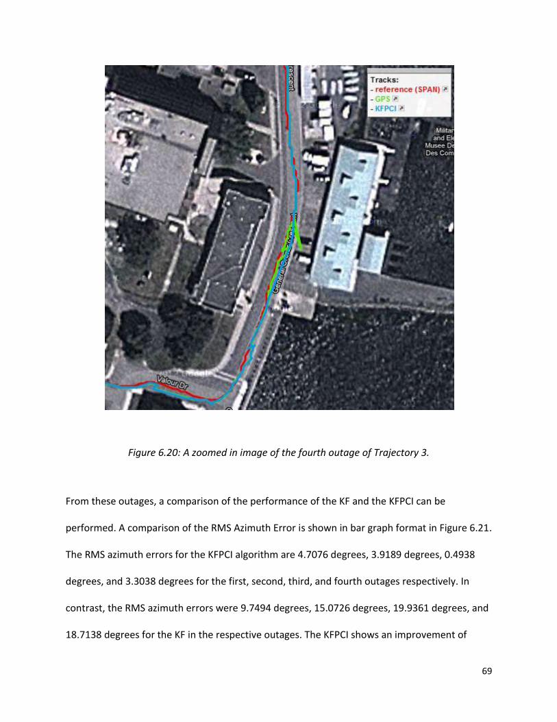
69
Figure 6.20: A zoomed in image of the fourth outage of Trajectory 3.
From these outages, a comparison of the performance of the KF and the KFPCI can be
performed. A comparison of the RMS Azimuth Error is shown in bar graph format in Figure 6.21.
The RMS azimuth errors for the KFPCI algorithm are 4.7076 degrees, 3.9189 degrees, 0.4938
degrees, and 3.3038 degrees for the first, second, third, and fourth outages respectively. In
contrast, the RMS azimuth errors were 9.7494 degrees, 15.0726 degrees, 19.9361 degrees, and
18.7138 degrees for the KF in the respective outages. The KFPCI shows an improvement of

70
51.7% in the first outage, 74.0% in the second outage, 97.5% in the third outage, and 82.34% in
the fourth outage.
Figure 6.21: RMS Azimuth Error for Trajectory 3.
The bar graph in Figure 6.22 shows the maximum azimuth error for each outage in Trajectory 3.
The maximum azimuth error in the KF PCI algorithm was found to be 9.826 degrees for the first
outage, 5.878 degrees for the second outage, 1.4895 degrees for the third outage, and 6.0395
degrees in the fourth outage. In contrast, the maximum azimuth errors for the KF were found
to be 15.2935 degrees for the first outage, 17.7067 degrees for the second outage, 20.5468
degrees for the third outage, and 19.0917 degrees for the fourth outage. The KFPCI showed an
improvement in the maximum azimuth error by 35.75%, 66.9%, 92.75%, and 68.37% for each of
the respective outages.
0
5
10
15
20
25
1 2 3 4
Azi
mu
th E
rro
r in
de
gre
es
Outage Number
RMS Azimuth Error
KF RMSAzimuth Error
KFPCI RMS Azimuth Error

71
Figure 6.22: Maximum Azimuth Errors in Trajectory 3.
Due to the dependency of the azimuth in the calculation of the position, an improvement in the
azimuth results in an improvement in the calculation of the position. A bar graph showing the
RMS errors in the position error is shown in Figure 6.23. The KFPCI algorithm shows RMS errors
of 4.8085 meters, 3.8566 meters, 2.2094 meters, and 3.7094 meters for the first through to
fourth outages respectively. In contrast, the KF algorithm shows RMS errors of 5.3958 meters,
6.2246, 2.7432, and 3.7686 meters for each of the respective outages. For each of the
respective outages, the KFPCI algorithm shows improvements of 10.89%, 38.04%, 19.46% and
1.57%.
0
5
10
15
20
25
1 2 3 4
Azi
mu
th E
rro
r in
de
gre
es
Outage Number
Max Azimuth Error
KF Max Azimuth Error
KFPCI Max Azimuth Error
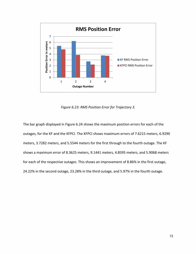
72
Figure 6.23: RMS Position Error for Trajectory 3.
The bar graph displayed in Figure 6.24 shows the maximum position errors for each of the
outages, for the KF and the KFPCI. The KFPCI shows maximum errors of 7.6215 meters, 6.9290
meters, 3.7282 meters, and 5.5544 meters for the first through to the fourth outage. The KF
shows a maximum error of 8.3625 meters, 9.1441 meters, 4.8595 meters, and 5.9068 meters
for each of the respective outages. This shows an improvement of 8.86% in the first outage,
24.22% in the second outage, 23.28% in the third outage, and 5.97% in the fourth outage.
0
1
2
3
4
5
6
7
1 2 3 4
Po
siti
on
Err
or
in m
ete
rs
Outage Number
RMS Position Error
KF RMS Position Error
KFPCI RMS Position Error

73
Figure 6.24: Maximum Position Error for each outage in Trajectory 3
6.4 Trajectory 4
The fourth trajectory was performed in the marching square at RMC, and is depicted in Figure
6.25. Starting from a point within the marching square, the robot moved diagonally towards the
southern edge of the marching square. It would proceed to move along the edges of the
marching square. After progressing a few meters along the north side, the robot turned right
approximately 30 degrees and maintained a straight path towards the southern edge of the
marching square. The robot then proceeded along the southern and eastern edge of the
marching square. After progressing a few meters on the northern edge, the robot moved on an
angle towards the starting point. The robot reached a maximum speed of 0.8825 m/s, and the
vehicle was always in motion. The trajectory was done in an open sky environment, and three,
0
1
2
3
4
5
6
7
8
9
10
1 2 3 4
Po
siti
on
Err
or
in m
ete
rs
Outage Number
Max Position Error
KF Max Position Error
KFPCI Max Position Error
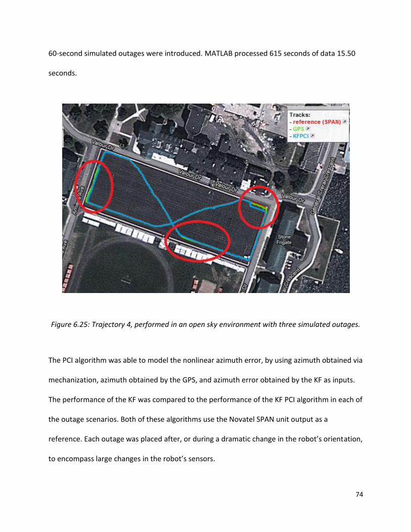
74
60-second simulated outages were introduced. MATLAB processed 615 seconds of data 15.50
seconds.
Figure 6.25: Trajectory 4, performed in an open sky environment with three simulated outages.
The PCI algorithm was able to model the nonlinear azimuth error, by using azimuth obtained via
mechanization, azimuth obtained by the GPS, and azimuth error obtained by the KF as inputs.
The performance of the KF was compared to the performance of the KF PCI algorithm in each of
the outage scenarios. Both of these algorithms use the Novatel SPAN unit output as a
reference. Each outage was placed after, or during a dramatic change in the robot’s orientation,
to encompass large changes in the robot’s sensors.

75
A close up of the first outage is depicted in Figure 6.26. This outage was placed at the first 90
degree turn the robot faces in its trajectory. This turn encompasses drastic changes in the
gyroscope readings of the robot.
Figure 6.26: A zoomed in image of the first outage in Trajectory 4.
The second outage, depicted in Figure 6.27, occurs at the end of the diagonal trajectory across
the marching square. This includes a relatively straight path followed by a 30 degree turn to the
right. The robot proceeds to move along the southern edge of the marching square for the
remainder of the outage.

76
Figure 6.27: A zoomed in image of the second outage of Trajectory 4.
A zoomed in image of the third outage is displayed in Figure 6.28. The outage includes a 90
degree left turn after the robot has progressed along the eastern edge of the marching square.
The 90 degree turn includes dramatic changes in the z-axis gyroscope readings.
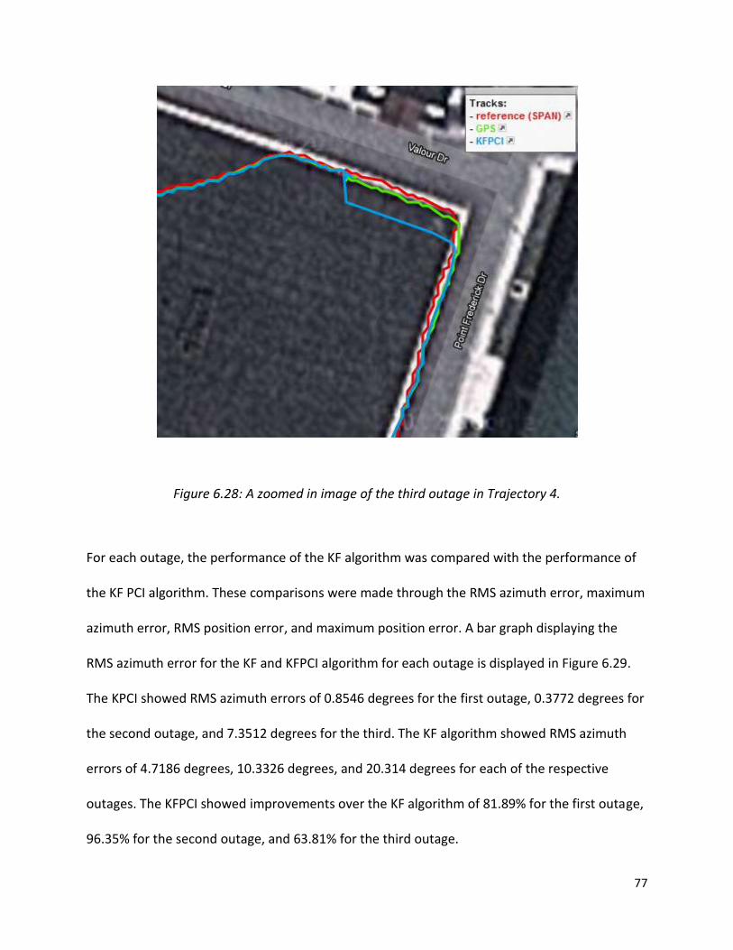
77
Figure 6.28: A zoomed in image of the third outage in Trajectory 4.
For each outage, the performance of the KF algorithm was compared with the performance of
the KF PCI algorithm. These comparisons were made through the RMS azimuth error, maximum
azimuth error, RMS position error, and maximum position error. A bar graph displaying the
RMS azimuth error for the KF and KFPCI algorithm for each outage is displayed in Figure 6.29.
The KPCI showed RMS azimuth errors of 0.8546 degrees for the first outage, 0.3772 degrees for
the second outage, and 7.3512 degrees for the third. The KF algorithm showed RMS azimuth
errors of 4.7186 degrees, 10.3326 degrees, and 20.314 degrees for each of the respective
outages. The KFPCI showed improvements over the KF algorithm of 81.89% for the first outage,
96.35% for the second outage, and 63.81% for the third outage.

78
Figure 6.29: RMS azimuth errors for Trajectory 4.
The maximum azimuth errors are displayed in the bar graph in Figure 6.30. For the first outage,
the KF PCI showed a maximum azimuth error of 2.0635 degrees, while the KF algorithm showed
an error of 6.0663 degrees. The second outage showed a maximum error of 1.4182 degrees for
the KF PCI algorithm, and 10.6777 degrees for the KF algorithm. The third outage showed
maximum errors for 34.4878 degrees for the KFPCI algorithm, and 51.2647 degrees for the third
outage. The KFPCI showed improvements of 65.98%, 86.72% and 32.73% over the KF for each
of the respective outages.
0
5
10
15
20
25
1 2 3
Azi
mu
th E
rro
r in
de
gre
es
Outage Number
RMS Azimuth Error
KF RMS Azimuth Error
KFPCI RMS Azimuth Error

79
Figure 6.30: Maximum azimuth errors for Trajectory 4.
An improvement in the azimuth results in an improvement in the calculation of the position, as
the calculation of the position is dependent on the azimuth. The RMS position errors for each
outage are displayed in Figure 6.31. The KFPCI showed RMS position errors of 1.065 meters,
1.232 meters, and 3.1131 meters for the first, second, and third outages respectively. The KF
showed RMS position errors of 1.7043 meters, 1.9158 meters, and 3.947 meters for each of the
respective outages. The KFPCI algorithm showed improvements over the KF algorithm by
37.51%, 35.69%, and 21.13% for each of the respective outages.
0
10
20
30
40
50
60
1 2 3
Azi
mu
th E
rro
r in
de
gre
es
Outage Number
Max Azimuth Error
KF Max Azimuth Error
KFPCI Max Azimuth Error

80
Figure 6.31: RMS position errors for Trajectory 4.
A bar graph displaying the maximum position errors is shown in Figure 6.32. The KF PCI
algorithm shows maximum position errors of 1.4215 meters for the first outage, 2.8823 meters
for the second outage, and 3.9227 for the third outage. In contrast, the KF shows maximum
position errors of 2.9325 meters, 4.1698 meters, and 6.9228 meters for each of the respective
outages. The KFPCI shows an improvement over the KF algorithm of 51.53%, 30.88% and
43.39% for each of the respective outages.
0
0.5
1
1.5
2
2.5
3
3.5
4
4.5
1 2 3
Po
siti
on
Err
or
in m
ete
rs
Outage Number
RMS Position Error
KF RMS Position Error
KFPCI RMS Position Error
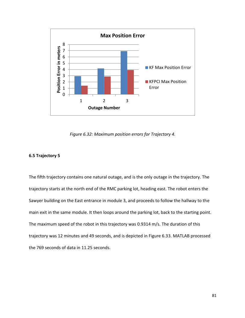
81
Figure 6.32: Maximum position errors for Trajectory 4.
6.5 Trajectory 5
The fifth trajectory contains one natural outage, and is the only outage in the trajectory. The
trajectory starts at the north end of the RMC parking lot, heading east. The robot enters the
Sawyer building on the East entrance in module 3, and proceeds to follow the hallway to the
main exit in the same module. It then loops around the parking lot, back to the starting point.
The maximum speed of the robot in this trajectory was 0.9314 m/s. The duration of this
trajectory was 12 minutes and 49 seconds, and is depicted in Figure 6.33. MATLAB processed
the 769 seconds of data in 11.25 seconds.
0
1
2
3
4
5
6
7
8
1 2 3
Po
siti
on
Err
or
in m
eter
s
Outage Number
Max Position Error
KF Max Position Error
KFPCI Max Position Error
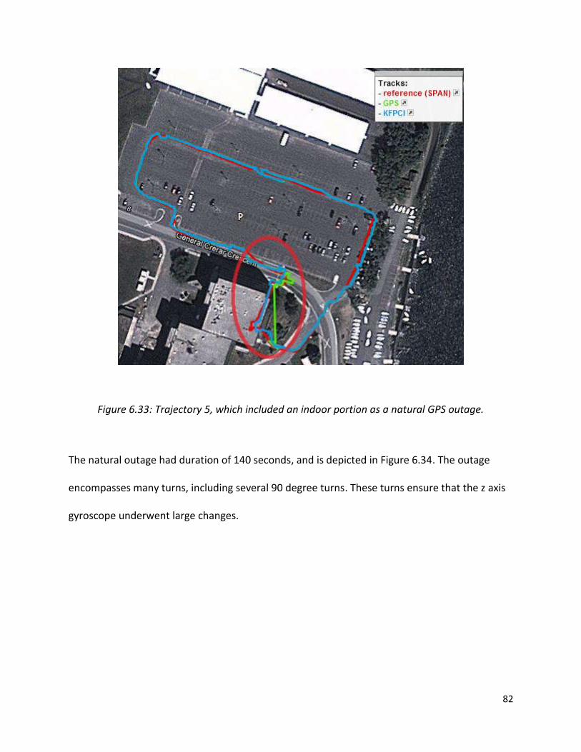
82
Figure 6.33: Trajectory 5, which included an indoor portion as a natural GPS outage.
The natural outage had duration of 140 seconds, and is depicted in Figure 6.34. The outage
encompasses many turns, including several 90 degree turns. These turns ensure that the z axis
gyroscope underwent large changes.
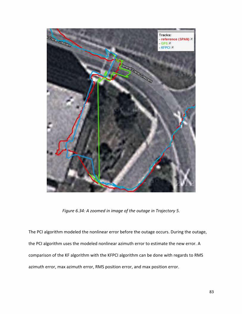
83
Figure 6.34: A zoomed in image of the outage in Trajectory 5.
The PCI algorithm modeled the nonlinear error before the outage occurs. During the outage,
the PCI algorithm uses the modeled nonlinear azimuth error to estimate the new error. A
comparison of the KF algorithm with the KFPCI algorithm can be done with regards to RMS
azimuth error, max azimuth error, RMS position error, and max position error.

84
A bar graph showing the RMS azimuth error is shown in Figure 6.35. One can note the RMS
azimuth error for the KFPCI during this outage is significantly less than the RMS azimuth error
for the KF. During this outage, the RMS azimuth error for the KFPCI algorithm was 2.8465
degrees, while it was 10.8016 degrees for the KF algorithm. The KFPCI algorithm shows a
73.65% improvement to the KF algorithm.
Figure 6.35: RMS Azimuth Error for Trajectory 5.
The maximum azimuth error for Trajectory 5 is shown in the bar graph in Figure 6.36. Similar to
the RMS azimuth error, the KFPCI algorithm results in a smaller value in the error. The KFPCI
algorithm has a maximum azimuth error of 9.9076 degrees, while the KF algorithm has an error
of 12.9845 degrees. The KFPCI algorithm shows a 29.93% improvement over the KF algorithm.
0
2
4
6
8
10
12
1
Azi
mu
th E
rro
r in
de
gre
es
Outage Number
RMS Azimuth Error
KF RMS Azimuth Error
KFPCI RMS Azimuth Error

85
Figure 6.36: Maximum Azimuth Error for Trajectory 5.
An improvement in the azimuth results in an improvement in the calculation of the position,
due to the dependency of the azimuth on the calculation of the position. A bar graph displaying
the RMS position error is depicted in Figure 6.37. For this outage, the KFPCI had an RMS
position error of 2.9348 meters, while the KF algorithm resulted in an error of 15.9171 meters.
The KFPCI algorithm showed an improvement of 81.56% over the KF algorithm.
0
2
4
6
8
10
12
14
1
Azi
mu
th E
rro
r in
de
gre
es
Outage Number
Max Azimuth Error
KF Max Azimuth Error
KFPCI Max Azimuth Error
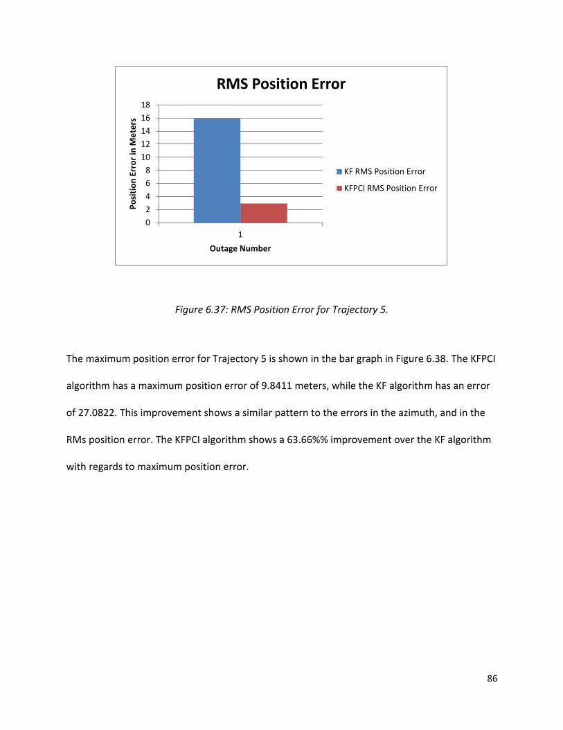
86
Figure 6.37: RMS Position Error for Trajectory 5.
The maximum position error for Trajectory 5 is shown in the bar graph in Figure 6.38. The KFPCI
algorithm has a maximum position error of 9.8411 meters, while the KF algorithm has an error
of 27.0822. This improvement shows a similar pattern to the errors in the azimuth, and in the
RMs position error. The KFPCI algorithm shows a 63.66%% improvement over the KF algorithm
with regards to maximum position error.
0
2
4
6
8
10
12
14
16
18
1
Po
siti
on
Err
or
in M
ete
rs
Outage Number
RMS Position Error
KF RMS Position Error
KFPCI RMS Position Error
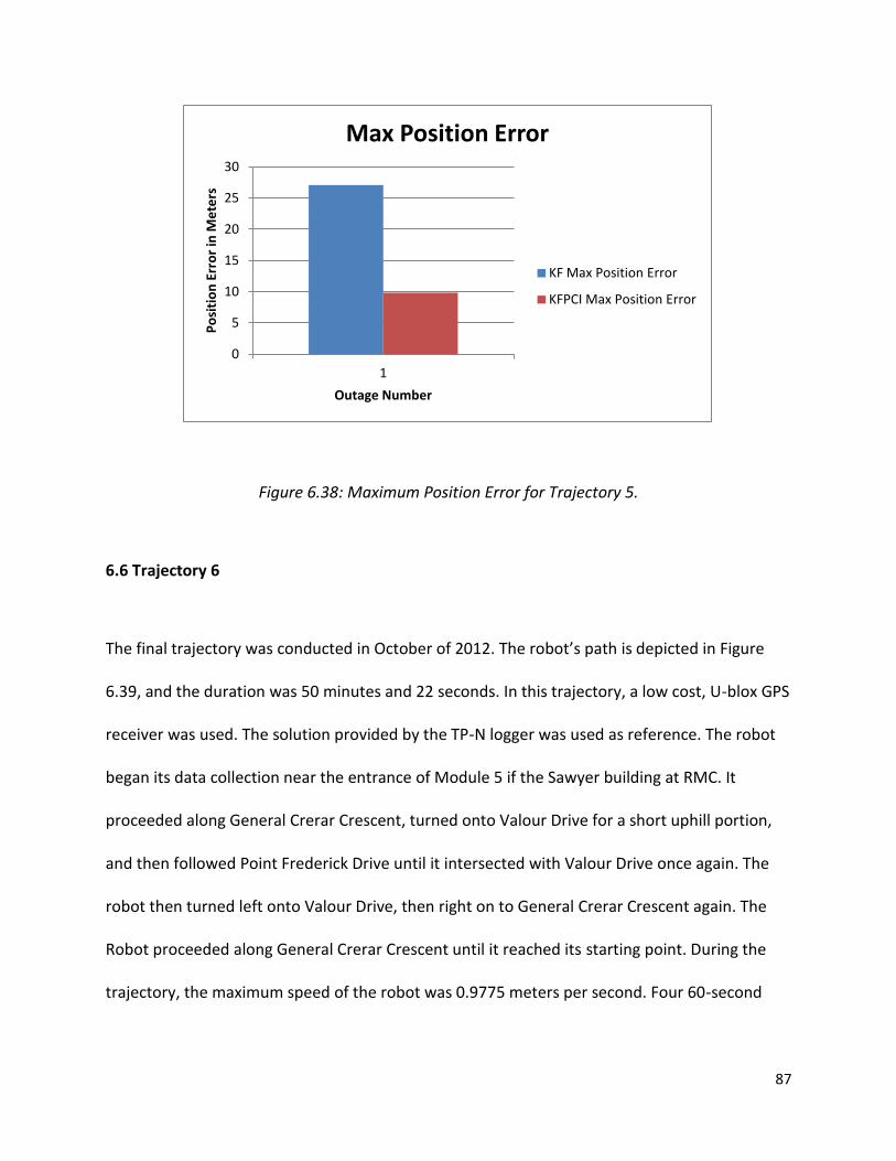
87
Figure 6.38: Maximum Position Error for Trajectory 5.
6.6 Trajectory 6
The final trajectory was conducted in October of 2012. The robot’s path is depicted in Figure
6.39, and the duration was 50 minutes and 22 seconds. In this trajectory, a low cost, U-blox GPS
receiver was used. The solution provided by the TP-N logger was used as reference. The robot
began its data collection near the entrance of Module 5 if the Sawyer building at RMC. It
proceeded along General Crerar Crescent, turned onto Valour Drive for a short uphill portion,
and then followed Point Frederick Drive until it intersected with Valour Drive once again. The
robot then turned left onto Valour Drive, then right on to General Crerar Crescent again. The
Robot proceeded along General Crerar Crescent until it reached its starting point. During the
trajectory, the maximum speed of the robot was 0.9775 meters per second. Four 60-second
0
5
10
15
20
25
30
1
Po
siti
on
Err
or
in M
ete
rs
Outage Number
Max Position Error
KF Max Position Error
KFPCI Max Position Error

88
simulated outages were used in this trajectory. The MATLAB code took 30.16 seconds to
process 3022 seconds of data.
Figure 6.39: Trajectory 6, performed in an open sky environment with 4 simulated outages.
The PCI algorithm was used to model the nonlinear azimuth errors while GPS is still available.
When the GPS signals are deemed unreliable, the KF PCI algorithm utilized the nonlinear
azimuth error model to predict and estimate the nonlinear error for the azimuth during the GPS
outage. The simulated outages are placed in locations encompassing a majority of scenarios
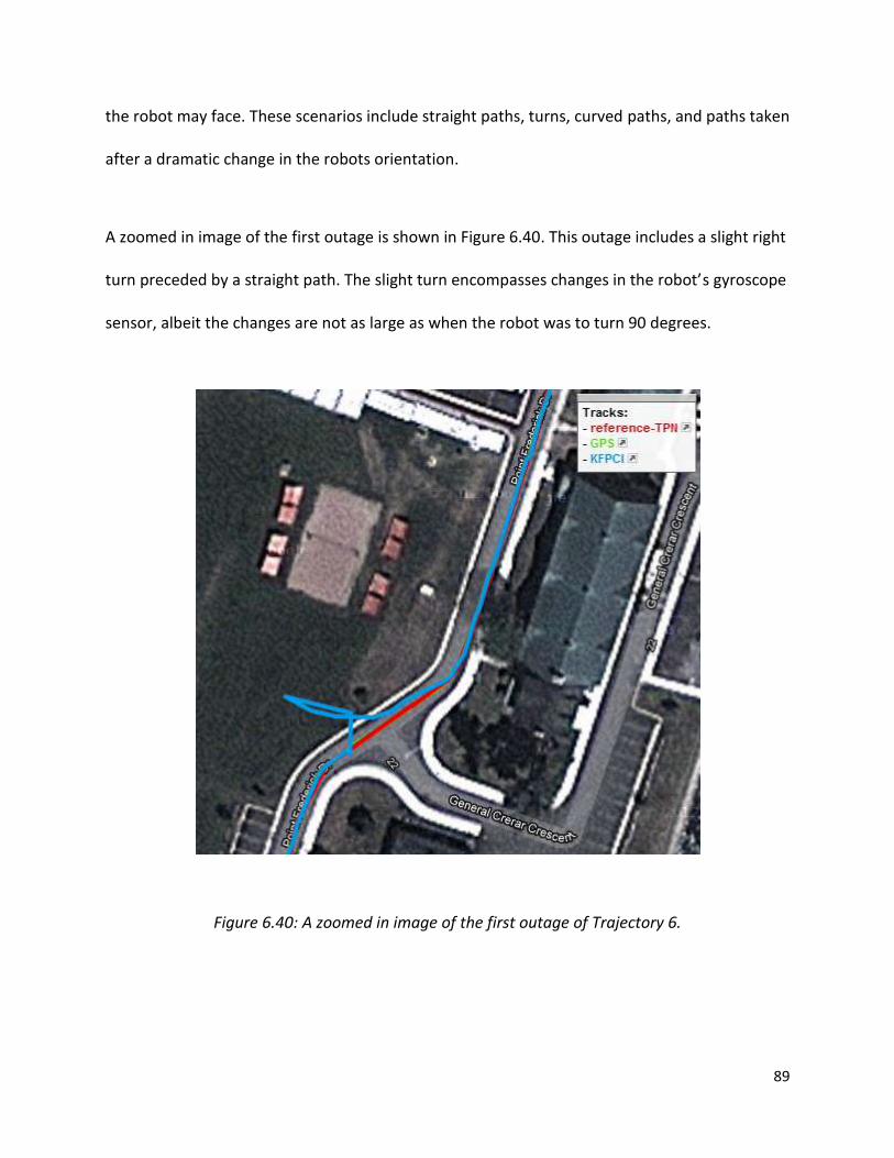
89
the robot may face. These scenarios include straight paths, turns, curved paths, and paths taken
after a dramatic change in the robots orientation.
A zoomed in image of the first outage is shown in Figure 6.40. This outage includes a slight right
turn preceded by a straight path. The slight turn encompasses changes in the robot’s gyroscope
sensor, albeit the changes are not as large as when the robot was to turn 90 degrees.
Figure 6.40: A zoomed in image of the first outage of Trajectory 6.

90
The second outage, depicted in Figure 6.41, encompasses a relatively straight path. The
changes gyroscope readings for this portion of the trajectory were relatively small, in
comparison to other outages. The deviance in the actual trajectory can still be noted.
Figure 6.41: A zoomed in image of the second outage in Trajectory 6.
The third outage is depicted in Figure 6.42, and features a gradual 80 degree turn. This turn is
when the robot is traversing around “the point” at RMC.

91
Figure 6.42: A zoomed in image of the third outage of Trajectory 6.
The fourth outage is along a slightly curved path, which takes place sometime after a near right
angled turn. This outage is depicted in Figure 6.43, and was placed near the intersection of
General Crerar Crescent and Precision Drive.
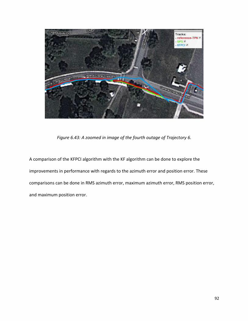
92
Figure 6.43: A zoomed in image of the fourth outage of Trajectory 6.
A comparison of the KFPCI algorithm with the KF algorithm can be done to explore the
improvements in performance with regards to the azimuth error and position error. These
comparisons can be done in RMS azimuth error, maximum azimuth error, RMS position error,
and maximum position error.

93
The RMS azimuth errors for trajectory 6 are graphed in Figure 6.44. The RMS azimuth error for
the KFPCI algorithm is less than the KF algorithm in all cases. Due to the low cost U-Blox GPS
receiver, the error in the azimuth is much higher than the error when using the NovaTel GPS
receiver. The RMS azimuth errors for outages 1 through 4 for the KFPCI algorithm are: 44.3356
degrees, 23.2427 degrees, 37.0051 degrees, and 19.4653 degrees respectively. With regards to
the KF algorithm, the respective RMS azimuth errors are: 112.7772 degrees, 81.7888 degrees,
61.4499 degrees, and 92.6305 degrees. The KFPCI algorithm showed improvements over the KF
algorithm for each outage. The percent difference between the KF algorithm and the KFPCI for
each respective outage was: 60.68%, 71.58%, 39.78% and 78.99%.
Figure 6.44: RMS Azimuth Errors for Trajectory 6.
0
20
40
60
80
100
120
1 2 3 4
Azi
mu
th E
rro
r in
de
gre
es
Outage Number
RMS Azimuth Error
KF RMS Azimuth Error
KFPCI RMS Azimuth Error

94
Similar to the RMS azimuth error, the maximum azimuth error shows improvement in the KFPCI
algorithm over the KF algorithm. The maximum azimuth error is graphed for each outage in
Figure 6.45. For the first outage, the maximum azimuth error was 93.0624 degrees for the
KFPCI algorithm, and 149.5127 degrees for the KF algorithm. The second outage showed
maximum azimuth errors of 47.9799 degrees for the KFPCI algorithm, and 112.6345 degrees for
the KF algorithm. The third outage showed errors of 53.2017 for the KFPCI and 83.7671 for the
KF. The final outage showed errors 55.4762 degrees for the KFPCI and 136.448 degrees for the
KF. The KFPCI showed improvements over the KF of 37.76%, 57.41%, 36.49%, and 59.34% for
the outages 1 through to 4, respectively.
Figure 6.45: Maximum Azimuth Errors for Trajectory 6.
0
20
40
60
80
100
120
140
160
1 2 3 4
Azi
mu
th E
rro
r in
de
gre
es
Outage Number
Max Azimuth Error
KF Max Azimuth Error
KFPCI Max Azimuth Error
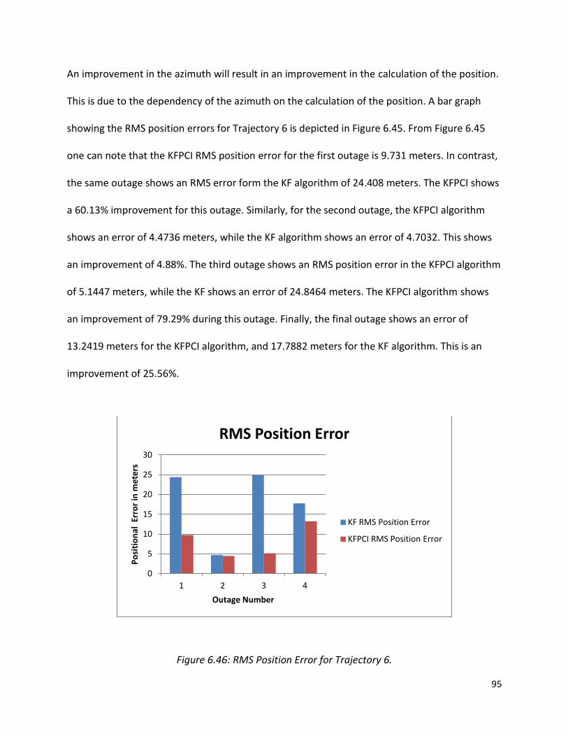
95
An improvement in the azimuth will result in an improvement in the calculation of the position.
This is due to the dependency of the azimuth on the calculation of the position. A bar graph
showing the RMS position errors for Trajectory 6 is depicted in Figure 6.45. From Figure 6.45
one can note that the KFPCI RMS position error for the first outage is 9.731 meters. In contrast,
the same outage shows an RMS error form the KF algorithm of 24.408 meters. The KFPCI shows
a 60.13% improvement for this outage. Similarly, for the second outage, the KFPCI algorithm
shows an error of 4.4736 meters, while the KF algorithm shows an error of 4.7032. This shows
an improvement of 4.88%. The third outage shows an RMS position error in the KFPCI algorithm
of 5.1447 meters, while the KF shows an error of 24.8464 meters. The KFPCI algorithm shows
an improvement of 79.29% during this outage. Finally, the final outage shows an error of
13.2419 meters for the KFPCI algorithm, and 17.7882 meters for the KF algorithm. This is an
improvement of 25.56%.
Figure 6.46: RMS Position Error for Trajectory 6.
0
5
10
15
20
25
30
1 2 3 4
Po
siti
on
al E
rro
r in
me
ters
Outage Number
RMS Position Error
KF RMS Position Error
KFPCI RMS Position Error

96
The KFPCI algorithm shows improvements for the maximum position error over the KF
algorithm, as depicted by the bar graph in Figure 6.46. For the first outage, an improvement of
66.96% can be seen. The KFPCI algorithm yields a maximum error of 16.0441 meters, while the
KF algorithm’s maximum error was 48.5595 meters. The second outage shows an improvement
of 5.21%. The KFPCI algorithm shows a maximum error of 8.7874 meters, while the KF
algorithm shows an error of 9.27 meters. The third outage shows the largest improvement of
the trajectory, of 84.10%. Use of the KFPCI algorithm resulted in a maximum error of 7.9029
meters, while the KF algorithm shows an error of 49.7109 meters. The final outage shows an
improvement of 23.60% in the maximum error. The KFPCI algorithm produces a maximum error
of 25.52 meters, while the KF algorithm produces a maximum error of 33.4142 meters.
Figure 6.47: Maximum Position Error for Trajectory 6.
0
10
20
30
40
50
60
1 2 3 4
Po
siti
on
al E
rro
r in
me
ters
Outage Number
Max Position Error
KF Max Position Error
KFPCI Max Position Error

97
6.7 Summary of Results
A summary of the results for all 6 trajectories is depicted in Table 6.1. Each column represents
the average error among the outages for each trajectory. From Table 6.1, one can note that the
KFPCI reduces the azimuth and position error more than the KF. This is due to the modelling of
the nonlinear portions of the azimuth error, which are not modelled in the stand alone KF. The
nonlinear modelling of the residual azimuth error, which was modelled by the PCI, results in a
reduction in the overall azimuth error. In turn, the reduction in the azimuth error has lead to a
reduction in the position error, due to the calculation dependency of the position on the
azimuth.
In most cases, the first outage for each trajectory would provide the smallee error in azimuth
and position for both the KF and the KFPCI than the second outage. This is due to the gyroscope
bias drift, as explained in Section 2.4.1. The only exception to this is in Trajectory 2, where the
first and second outages show approximately the same RMS azimuth error. This may be due to
the robot moving on a straight line path during the second outage.
In all experiments, the maximum speed of the robot would never reach above 1.1 m/s. This low
speed would classify the robot as having low mobility. At lower speeds, the azimuth error is
generally lower than that of a civilian sedan, which reaches speeds of 60 to 100 km/h.
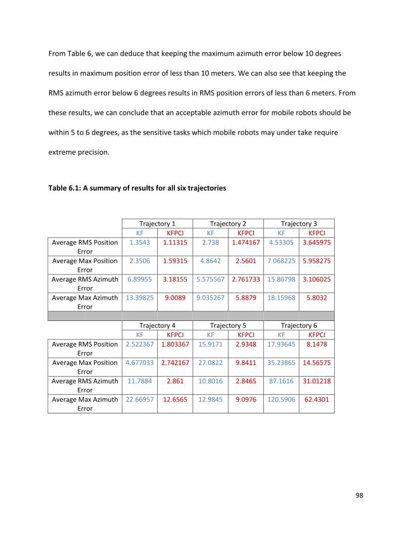
98
From Table 6, we can deduce that keeping the maximum azimuth error below 10 degrees
results in maximum position error of less than 10 meters. We can also see that keeping the
RMS azimuth error below 6 degrees results in RMS position errors of less than 6 meters. From
these results, we can conclude that an acceptable azimuth error for mobile robots should be
within 5 to 6 degrees, as the sensitive tasks which mobile robots may under take require
extreme precision.
Table 6.1: A summary of results for all six trajectories
Trajectory 1 Trajectory 2 Trajectory 3
KF KFPCI KF KFPCI KF KFPCI
Average RMS Position Error
1.3543 1.11315 2.738 1.474167 4.53305 3.645975
Average Max Position Error
2.3506 1.59315 4.8642 2.5601 7.068225 5.958275
Average RMS Azimuth Error
6.89955 3.18155 5.575567 2.761733 15.86798 3.106025
Average Max Azimuth Error
13.39825 9.0089 9.035267 5.8879 18.15968 5.8032
Trajectory 4 Trajectory 5 Trajectory 6
KF KFPCI KF KFPCI KF KFPCI
Average RMS Position Error
2.522367 1.803367 15.9171 2.9348 17.93645 8.1478
Average Max Position Error
4.677033 2.742167 27.0822 9.8411 35.23865 14.56575
Average RMS Azimuth Error
11.7884 2.861 10.8016 2.8465 87.1616 31.01218
Average Max Azimuth Error
22.66957 12.6565 12.9845 9.0976 120.5906 62.4301
99
Chapter 7 - Concluding Remarks
7.1 Summary
As seen in Chapter 6, the KFPCI algorithm provided superior results to the KF algorithm for each
of the outages described in the six trajectories in terms of azimuth error and position error. The
results compared between the two algorithms were the RMS position error, the maximum
position error, the RMS azimuth error, and the maximum azimuth error. When combining the
low cost XBow IMU with the OEM-4 GPS Receiver, the KFPCI algorithm showed average
improvements of 30.76%, 34.71%, 66.76%, and 53.58% over the KF for each of the respective
errors. When combining the low cost XBow IMU with the low cost U-blox receiver, the KFPCI
algorithm showed average improvements of 42.47%, 44.96%, 62.75%, and 47.75% over the KF
for each of the respective errors. We can conclude the azimuth error for mobile robots should
be less than 6 degrees, as position accuracy is a necessity for the sensitive tasks the robot may
participate in. The azimuth error of 6 degrees results in a position error of less than 6 meters.
7.2 Contributions
The main contribution from this research is implementation of the Kalman Filter augmented
with Parallel Cascade Identification for modeling azimuth error. The research provided in [4] for
cars and land based vehicles was implemented into the mobile platform.

100
7.3 Recommendations for Future Work
This thesis dealt with the integration of 2D RISS/GPS, and the results of the trajectories were
achieved via post processing. It is recommended that 3D RISS/GPS integration be pursued, to
investigate whether 3D integration is superior to the 2D integration in hills and valleys. To
implement 3D RISS, two accelerometers are used in the x and y axes to measure pitch and roll,
as explained in [13]. It is also recommended to investigate the real time application of the KFPCI
algorithm, as the PCI algorithm results in a larger computation time.
While Kalman Filtering is a good technique for estimating the error states of the position and
attitude of the moving platform, it is limited due to the linearization of the errors. The Particle
Filter does not linearize errors, and is designed to work with nonlinear error models. It is
recommended that the use of the Particle Filter in the mobile robot platform should be
pursued. One of the main limitations of the Particle Filter is that its error increases as the state
dimension increases. As stated in [43], this is because the number of particles increase
exponentially with the dimension of the state space.
As mentioned in Chapter 2, Atia was able to integrate RISS and WiFi to form an integrated
navigation solution for indoor environments. For future research, one can pursue the
integration of GPS, WiFi, and RISS, so that an integrated solution can be available for both
indoor and outdoor environments.

101
References
[1] D. W. Gage, “UGV History 101: A Brief History of Unmanned Ground Vehicle Development
Efforts,” in Unmanned Systems Magazine, vol. 13, No. 3. pp. 1-9, 1995.
[2] Unmanned Air Vehicle (UAV), Transport Canada, [online] May, 2010,
http://www.tc.gc.ca/eng/civilaviation/standards/general-recavi-brochures-uav-2270.htm
(Accessed: February 2012).
[3] C. DesMarais, “Domestic Robots: High-Tech House Helpers,” PCWorld, [online] Apr 16,
2012,
http://www.pcworld.com/article/253882/domestic_robots_high_tech_house_helpers.ht
ml (Accessed: February 2013).
[4] U. Iqbal et al, “Nonlinear Modeling of Azimuth Error for 2D Car Navigation Using Parallel
Cascade Identification Augmented with Kalman Filtering,” International Journal of
Navigation and Observation, Vol. 2010, pp. 1-13, 2010.
[5] Dictionary.com, "navigation," in Collins English Dictionary - Complete & Unabridged 10th
Edition. Source location: HarperCollins Publishers.
http://dictionary.reference.com/browse/navigation. Available:
http://dictionary.reference.com. (Accessed: June 11, 2013).
[6] Navigation - History of Navigation, ABC, [online] 2011,
http://www.abc.net.au/navigators/navigation/history.htm (Accessed: February 2012).
[7] F. Van Diggelen, A-GPS: Assisted GPS, GNSS, and SBAS, Artech House, 2009, pp. 9 - 13.

102
[8] Space Segment, GPS Government. [online] February 12, 2013,
http://www.gps.gov/systems/gps/space/ (Accessed: March, 2013) .
[9] J. A. Farrel and M. Barth, The Global Positioning System and Inertial Navigation, McGraw-
Hill, 1999, pp 5 - 11.
[10] T. Karamat, The GPS Positioning System, an Introduction, class notes for EE523,
Department of Electrical and Computer Engineering, Royal Military College of Canada,
September, 2011.
[11] Y. Zhao, Vehicle Location and Navigation Systems, Michigan, Artech House, 1997, pp. 63 -
76.
[12] A. El-Rabbany, Introduction to GPS: The Global Positioning System, class notes,
Department of Civil Engineering, Ryerson University, 2002.
[13] U. Iqbal, “MULTI-SENSOR DATA FUSION FOR VEHICULAR NAVIGATION APPLICATIONS,”
PHD thesis, Queen’s University, 2012.
[14] A. Noureldin et al. Fundamentals of Inertial Navigation, Satellite-based Positioning and
their Integration, Springer, 2013.
[15] E. North, “POSITIONING AND NAVIGATION OF WHEELED MOBILE ROBOTS IN
CHALLENGING GPS ENVIRONMENTS” MASc Thesis, Royal Military College of Canada, 2009.
[16] A. Noureldin. “Integrated Navigation Systems,” class notes for EE523, Department of
Electrical and Computer Engineering, Royal Military College of Canada, September 2012.

103
[17] J. A. Farrel et al., The Global Positioning System and Inertial Navigation, McGraw-Hill,
2000, pp 21-24.
[18] Y. Zhao, Vehicle Location and Navigation Systems, Artech House, 1997, pp. 43 - 56.
[19] K. R. Britting, Inertial Navigation Systems Analysis, Artech House, 2010, pp. 1 - 4.
[20] B-J. Yoon et al., UGV (Unmanned Ground Vehicle) Navigation Method Using GPS and
Compass in SICE-ICASE International Joint Conference, 2006, pp. 3621 – 3625.
[21] S. Sukkarieh et al., “A High Integrity IMU/GPS Navigation Loop for Autonomous Land
Vehicle Applications,” IEEE Transactions on Instrumentation and Automation. Vol. 15, No
3, pp. 572 - 578, June 1999.
[22] T. Aono, “Positioning of Vehicle on Undulating Ground Using GPS and Dead Reckoning,”
Proceedings of 1998 IEEE international Conference on Robotics and Automation, Vol 4. Pp.
3443 – 3448, May 1998.
[23] W. Abdelfatah “REAL-TIME EMBEDDED SYSTEM DESIGN AND REALIZATION FOR
INTEGRATED NAVIGATION SYSTEMS” MASc Thesis, Queen’s University, 2010.
[24] M. Atia et al, “Particle Filter-based WiFi-Aided Reduced Inertial Sensors Navigation System
for Indoor and GPS denied Environments,” Hindawi International Journal of Navigation
and Observation, Vol. 2009, pp. 1-12, 2012.
104
[25] C-Y. Chan, “Magnetic Sensing as Position Reference System for Ground Vehicle Control,”
IEEE Transactions on Instrumentation and Measurement, vol. 51, No. 1, pp. 43 – 52,
February 2002.
[26] Z. Shen “NONLINEAR MODELING OF INERTIAL ERRORS BY FAST ORTHOGONAL SEARCH
ALGORITHM FOR LOW COST VEHICULAR NAVIGATION” PHD Thesis, Queen’s University,
2012.
[27] A. Noureldin et al. “Performance Enhancement of MEMS-Based INS/GPS Integration for
Low Cost Navigation Applications” IEEE Transactions on Vehicular Technology, vol. 58, pp.
1077 – 1096, March 2009.
[28] U. Iqbal et al. “Experimental Results on an Integrated GPS and Multisensor System for
Land Vehicle Positioning,” Hindawi International Journal of Navigation and Observation,
Vol. 2009. pp. 1 – 18, 2009.
[29] J. Georgy “Low Cost Three-Dimensional Navigation Solution for RISS/GPS Integration Using
Mixture Particle Filter”, IEEE Transactions on Vehicular Technology. vol. 59, No. 2, pp. 599
– 615, February 2010.
[30] M. Atia et al. “Real-time implementation of mixture particle filter for 3D RISS/GPS
integrated navigation solution” Electronics Letters, vol. 46, No. 15, pp. 1083 – 1084, July
2010.

105
[31] J. Georgy et al. “Modeling the Stochastic Drift of a MEMS based gyro in gyro/odometer/GPS
integrated navigation” IEEE Transactions on Vehicular Technology, Vol. 11, No. 4, pp. 856
– 872, December 2010.
[32] J. Georgy, “ADVANCED NONLINEAR TECHNIQUES FOR LOW COST LAND VEHICLE
NAVIGATION” PHD Thesis, Queen’s University, 2010.
[33] M. J. Korenberg, “Statistical Identification of parallel cascades of linear and nonlinear
systems,” Sixth IFAC Symposium on Identification and System Parameter Estimation, pp.
580-585, 1982.
[34] M. J. Korenberg, “Parallel Cascade Identification and kernel estimation for nonlinear
systems,” Annals of Biomedical Engineering, vol. 19, pp. 429-455, 1991.
[35] J. Georgy et al, “Low-Cost Three-Dimensional Navigation Solution for RISS/GPS Integration
Using Mixture Particle Filter,” IEEE Transactions on Vehicular Technology, vol. 59. No.2,
pp. 599 – 615, February 2010.
[36] M. J. Korenberg et al. "Parallel cascade identification as a means for automatically
classifying protein sequences into structure/function groups," Biological Cybernetics, vol.
81, pg 15-21, 2000.
[37] M. S. Grewal et al., Kalman Filtering: Theory and Practice Using MATLAB, 2nd ed., John
Wiley and Sons, 2001, pp 1 to 24.
[38] A. Noureldin. “Kalman Filter-An Introduction,” class notes for EE523, Department of
Electrical and Computer Engineering, Royal Military College of Canada, September 2012.

106
[39] IMU 6DOF Inertial Measurement Unit: Crossbow Technology Inc., Crossbow Technology
Inc., [online],
http://saba.kntu.ac.ir/eecd/ecourses/instrumentation/projects/reports/Poly%20Gyroscop
e/Producers/Crossbow/IMU/6020-0019-01_B_IMU300CC.pdf (Accessed: February 2013).
[40] Trusted Positioning Inc. “TPN Quick Start Manual ver. 1.0” September, 2012.
[41] HG1700 Inertial Measurement Unit: Honeywell Inc., Honeywell Inc., [online].
http://www51.honeywell.com/aero/common/documents/myaerospacecatalog-
documents/Missiles-Munitions/HG1700_Inertial_Measurement_Unit.pdf (Accessed:
February 2013).
[42] SPAN Technology System User Manual OM-20000062 Rev 7: NovaTel Inc., NovaTel Inc.,
http://webone.novatel.ca/assets/Documents/Manuals/om-20000062.pdf (Accessed:
February 2013).
[43] S. Thrun. “Particle Filters in Robotics” Proceedings of Uncertainty in AI (UAI), pp. 1-9,
2002.uments/Manuals/om-20000062.pdf} (Accessed: February 2013).