Frame Partitioning

in WiMax Mesh mode

by

Qutaiba Albluwi

A thesis submitted to the

School of Computing

in conformity with the requirements for

the degree of Master of Science

Queen’s University

Kingston, Ontario, Canada

October 2008

Copyright c© Qutaiba Albluwi, 2008

Abstract

WiMax or the IEEE 802.16 standard is one of the most promising broadband wireless

technologies nowadays. It is characterized by its high data rates, large coverage area,

flexible design and QoS support. The standard defines two modes of operation: Point-

to-Multi-Point (PMP) and the Mesh Mode. In the first mode, all nodes are connected

directly to the base station and communication is not allowed amongst nodes. In the

mesh mode, nodes are placed in an ad hoc manner communicating to neighbors and

relaying the traffic of other nodes. The goal of this thesis is to design a partitioning

scheme for the frame structure of the Mesh mode. Increasing the frame utilization

would result in better support for QoS applications and optimized resource allocation,

and thus revenue increase from the service provider’s perspective.

The mesh frame is divided into control and data, which are further divided into

centralized and distributed portions. We propose a novel and efficient scheme for par-

titioning the data subframe between the two schedulers. We use a Markovian model

that studies the system behavior in the long run, and provides predictions based on

analysis of previous window of frames. We further enhance the decision by tuning the

partitioning through statistical analysis of smaller windows to accommodate demand

changes. Our simulations show that the proposed scheme achieves high utilization

under different network and traffic conditions and decreases the packet overflow.

i

Dedication

To who taught me how to carry the pencil

... and how to rejoice for the sound it makes

To who inspired me to search for meanings

... and share them with the breeze

Before two decades you had a dream

... But now I have a dream!

I just want to see you smile

... And He embraces your hearts with peace

To my beloved parents

... I dedicate this work

ii

Acknowledgments

I would like to express my sincerest gratitude and thanks to my supervisor: Dr.

Hossam Hassanein for his continues academic support and for his nice treatment and

patience. He motivated me along the way by encouraging creative thinking and open-

ing my eyes upon different issues in the wireless field. I would like to thank also my

co-supervisor Dr. Najah Abu Ali (UAE University), who provided support for the

details in this thesis which include the algorithm design, and simulation analysis. Spe-

cial thanks are to my family, especially my parents , my two brothers and twin sisters

who were always inspirative and supportive. Without their prayers and emotional

support, this work would not have seen the light. The wonderful team in the TRL

lab will be always remembered with their excellent cooperative work and help. The

team was amazing. The over-night stays, day coffee breaks, and many of the daily

chats are memorable. Special thanks are to my dear colleague Bader Almanthari,

who read my thesis and generously provided many constructive comments. There

are other individuals who have helped me during my study period, but their names

are not listed here. Their support to me is too precious to be recorded in writing.

I am indebted to them for the rest of my life. Finally, I thank the members of the

School of Computing at Queens University for their nice program and for providing

such productive environment.

iii

Contents

Abstract i

Dedication ii

Acknowledgments iii

Contents iv

List of Tables vii

List of Figures viii

Acronyms ix

Abbreviations xiii

1 Introduction 11.1 Broadband Access Networks . . . . . . . . . . . . . . . . . . . . . . . 21.2 Broadband Wireless Access . . . . . . . . . . . . . . . . . . . . . . . 31.3 WiMax . . . . . . . . . . . . . . . . . . . . . . . . . . . . . . . . . . . 41.4 Motivation and Research Objectives . . . . . . . . . . . . . . . . . . . 71.5 Thesis Organization . . . . . . . . . . . . . . . . . . . . . . . . . . . . 9

2 Background 102.1 Overview of WiMax and its evolution . . . . . . . . . . . . . . . . . . 10

2.1.1 WiMax PMP Mode . . . . . . . . . . . . . . . . . . . . . . . . 132.1.2 WiMax Mesh Mode . . . . . . . . . . . . . . . . . . . . . . . . 16

2.2 Frame Structure in WiMax Mesh Mode . . . . . . . . . . . . . . . . . 192.2.1 Control subframe . . . . . . . . . . . . . . . . . . . . . . . . . 202.2.2 Data Subframe . . . . . . . . . . . . . . . . . . . . . . . . . . 23

2.3 Scheduling in WiMax Mesh Mode . . . . . . . . . . . . . . . . . . . . 242.3.1 Centralized Scheduling . . . . . . . . . . . . . . . . . . . . . . 25

iv

2.3.2 Coordinated Distributed Scheduling . . . . . . . . . . . . . . . 282.3.3 Uncoordinated Distributed Scheduling . . . . . . . . . . . . . 31

2.4 Related Work . . . . . . . . . . . . . . . . . . . . . . . . . . . . . . . 32

3 Frame Partitioning in WiMax Mesh Mode 353.1 Problem Description . . . . . . . . . . . . . . . . . . . . . . . . . . . 353.2 System Model . . . . . . . . . . . . . . . . . . . . . . . . . . . . . . . 37

3.2.1 Network Model . . . . . . . . . . . . . . . . . . . . . . . . . . 393.2.2 Bandwidth Requests . . . . . . . . . . . . . . . . . . . . . . . 40

3.3 Mathematical Model . . . . . . . . . . . . . . . . . . . . . . . . . . . 433.3.1 Preliminaries . . . . . . . . . . . . . . . . . . . . . . . . . . . 433.3.2 Coarse Window . . . . . . . . . . . . . . . . . . . . . . . . . . 453.3.3 Fine Window . . . . . . . . . . . . . . . . . . . . . . . . . . . 50

3.4 Prediction for optimal frame partitioning . . . . . . . . . . . . . . . . 543.4.1 Preliminaries . . . . . . . . . . . . . . . . . . . . . . . . . . . 543.4.2 Frame Partitioning with Gradual Increase . . . . . . . . . . . 563.4.3 Frame Partitioning with Maximal Increase . . . . . . . . . . . 57

3.5 Summary . . . . . . . . . . . . . . . . . . . . . . . . . . . . . . . . . 59

4 Performance Evaluation 634.1 Simulation Model . . . . . . . . . . . . . . . . . . . . . . . . . . . . . 63

4.1.1 Simulator . . . . . . . . . . . . . . . . . . . . . . . . . . . . . 634.1.2 Traffic Model . . . . . . . . . . . . . . . . . . . . . . . . . . . 644.1.3 Performance Metrics . . . . . . . . . . . . . . . . . . . . . . . 664.1.4 Simulation Parameters . . . . . . . . . . . . . . . . . . . . . . 69

4.2 Scheme Parameters Evaluation . . . . . . . . . . . . . . . . . . . . . 724.2.1 Coarse window Parameters . . . . . . . . . . . . . . . . . . . . 724.2.2 Fine Window . . . . . . . . . . . . . . . . . . . . . . . . . . . 74

4.3 Numerical Results . . . . . . . . . . . . . . . . . . . . . . . . . . . . . 784.3.1 Traffic Type . . . . . . . . . . . . . . . . . . . . . . . . . . . . 794.3.2 Frame Duration . . . . . . . . . . . . . . . . . . . . . . . . . . 814.3.3 Number of Nodes . . . . . . . . . . . . . . . . . . . . . . . . . 82

4.4 Summary . . . . . . . . . . . . . . . . . . . . . . . . . . . . . . . . . 84

5 Conclusion 865.1 Contributions . . . . . . . . . . . . . . . . . . . . . . . . . . . . . . . 865.2 Future Work . . . . . . . . . . . . . . . . . . . . . . . . . . . . . . . . 87

Bibliography 89

v

A Simulator Model Components 96A.1 Network Package . . . . . . . . . . . . . . . . . . . . . . . . . . . . . 97A.2 Frame Package . . . . . . . . . . . . . . . . . . . . . . . . . . . . . . 98A.3 Traffic Package . . . . . . . . . . . . . . . . . . . . . . . . . . . . . . 99A.4 Algorithm Package . . . . . . . . . . . . . . . . . . . . . . . . . . . . 99A.5 Math Package . . . . . . . . . . . . . . . . . . . . . . . . . . . . . . . 101

vi

List of Tables

2.1 802.16 PHY variants . . . . . . . . . . . . . . . . . . . . . . . . . . . 142.2 WiMax Modulation Schemes . . . . . . . . . . . . . . . . . . . . . . . 152.3 QoS Services supported by WiMax . . . . . . . . . . . . . . . . . . . 172.4 Frame Duration . . . . . . . . . . . . . . . . . . . . . . . . . . . . . . 20

4.1 Transmission Modes of IEEE 802.16 . . . . . . . . . . . . . . . . . . . 664.2 Fixed Simulation Parameters . . . . . . . . . . . . . . . . . . . . . . . 704.3 Variable Simulation Parameters . . . . . . . . . . . . . . . . . . . . . 714.4 Simulation Variables for Measuring Coarse Window Parameters . . . 724.5 Test Environments for Studying the Effect of the Fine Window . . . . 75

A.1 WiMax Traffic Model Parameters . . . . . . . . . . . . . . . . . . . . 100

vii

List of Figures

1.1 WiMAX Network Architecture . . . . . . . . . . . . . . . . . . . . . . 71.2 Illustration of the Thesis Problem . . . . . . . . . . . . . . . . . . . . 8

2.1 IEEE 802.16 Publications . . . . . . . . . . . . . . . . . . . . . . . . 112.2 IEEE 802.16 Protocol Stack . . . . . . . . . . . . . . . . . . . . . . . 122.3 IEEE 802.16 MAC PDU Format . . . . . . . . . . . . . . . . . . . . . 162.4 Mesh mode frame structure . . . . . . . . . . . . . . . . . . . . . . . 212.5 Scheduling network control frames . . . . . . . . . . . . . . . . . . . . 222.6 Structure of Control Subframe . . . . . . . . . . . . . . . . . . . . . . 232.7 Example of Centralized Scheduling . . . . . . . . . . . . . . . . . . . 26

3.1 Example of WiMax mesh network . . . . . . . . . . . . . . . . . . . . 413.2 Partitioning Algorithm Flow Chart . . . . . . . . . . . . . . . . . . . 443.3 Calculation of window sizes . . . . . . . . . . . . . . . . . . . . . . . 463.4 Demand Markov Chain . . . . . . . . . . . . . . . . . . . . . . . . . . 483.5 Calculation of PD Matrix . . . . . . . . . . . . . . . . . . . . . . . . . 493.6 Network State . . . . . . . . . . . . . . . . . . . . . . . . . . . . . . . 513.7 Calculation of PC and PS probability matrices . . . . . . . . . . . . . 533.8 Example of Fine Window Partitioning Decision . . . . . . . . . . . . 583.9 Frame Partitioning Algorithm with Gradual Increase . . . . . . . . . 613.10 Frame Partitioning Algorithm with Maximal Increase . . . . . . . . . 62

4.1 Optimum Coarse Window Size . . . . . . . . . . . . . . . . . . . . . . 734.2 Coarse Window Granularity . . . . . . . . . . . . . . . . . . . . . . . 744.3 Fine Window Effect . . . . . . . . . . . . . . . . . . . . . . . . . . . . 774.4 Fine Window Step Size . . . . . . . . . . . . . . . . . . . . . . . . . . 784.5 Scheme Comparison (Traffic Type) . . . . . . . . . . . . . . . . . . . 804.6 Scheme Comparison (Frame Duration) . . . . . . . . . . . . . . . . . 814.7 Scheme Comparison (Number of Nodes) . . . . . . . . . . . . . . . . 83

viii

Acronyms

AAS Adaptive Antenna System

ADSL Asymmetric Digital Subscriber Line

AES Advanced Encryption Standard

AMC Adaptive Modulation and Coding

ARQ Automatic Repeat Request

ATM Asynchronous Transfer Mode

BE Best Effort

BPSK Binary Phase Shift Keying

BS Base Station

BWA Broadband Wireless Access

CAC Call Admission Control

CID Connection Identifier

CPS Common Part Sublayer

ix

CS Convergence Sublayer

CSCF Centralized Scheduling Configuration

CSCH Centralized Scheduling

DL Down Link

DSCH Distributed Scheduling

DSL Digital Subscriber Line

ertPS Extended Real-Time Polling Service

FDD Frequency Division Duplex

FEC Forward Error Correction

FFT Fast Fourier Transform

H-FDD Half Duplex Frequency Division Duplex

HDSL High-bit-rate Digital Subscriber Line

HUMAN High Speed Unlicensed Metropolitan Area Network

IDSL ISDN Digital Subscriber Line

IE Information Element

IP Internet Protocol

LMDS Local Multipoint Distribution System

LOS Line of Sight

x

MAC Medium Access Control

MAN Metropolitan Area Network

MIB Management Information Base

MMDS Multichannel Multi-point Distribution System

MSH Mesh

NCFG Network Configuration

NENT Network Entry

NLOS None Line of Sight

nrtPS Non-Real-Time Polling Service

OFDM Orthogonal Frequency Division Multiplexing

OFDMA Orthogonal Frequency Division Multiple Access

PDU Protocol Data Unit

PHY Physical Layer

PMP Point to Multi-point

QAM Quadrature Amplitude Modulation

QoS Quality of Service

QPSK Quadrature Phase Shift Keying

rtPS Real Time Polling Service

xi

SAP Service Access Point

Sc Single Carrier

Sc-a Single Carrier Access

SDSL Symmetric Digital Subscriber Line

SDU Service Data Unit

SFID Service Flow Identifier

SS Subscriber Station

STC Space Time Coding

TDD Time Division Duplex

TDM Time Division Multiplexing

TDMA Time Division Multiple Access

U Utilization

UGS Unsolicited Grant Service

UL Up Link

VoIP Voice over IP

WiMax Worldwide Interoperability for Microwave Access

WirelessMAN Wireless Metropolitan Area Network

xii

Abbreviations

Abbrev. Description Units

LD Size of the data subframe symbolsLDC Size of the centralized scheduler in the data subframe symbolsLDD Size of the distributed scheduler in the data subframe symbolsLDmin Minimum value for LDC and LDD symbolsLDmax Maximum value for LDC and LDD symbolsWC Number of coarse windows windowsWF Number of fine windows in a coarse window windowsFc Number of frames per coarse window framesFf Number of frames per fine window framesλni The request of node n in the frame i symbolsλmax The maximum node request per frame symbolsλi The sum of all node requests for the frame i symbolsUi Utilization of frame i –δi Overflow probability of frame i –

xiii

Chapter 1

Introduction

The world today, undoubtedly speaks Wireless. The number of people today carrying

a cell phone is approximately 3.25 billion, which is three times the number of people

speaking Mandarin, the largest spoken language [45]. From the simple wireless hand-

sets used in video games to the complex satellite military communications, wireless

technologies show high penetration rates into many aspects of daily life. Generally,

wireless communication provides lower costs, wider support for users and more con-

venient access by supporting user mobility. One of the newest wireless broadband

access technologies is the IEEE 802.16, which is also known as WiMax standing for

Worldwide Interoperability for Microwave Access. In this work, we provide a novel

method for increasing the throughput of WiMax networks by finding an efficient

method for partitioning the frame through different schedulers. This work should be

of interest to service providers as it provides better utilization of the resources, which

would result in increased revenues. Before, providing the technical details, we will

start by giving a brief history of broadband access networks in general, and wireless

broadband access networks.

1

1.1 Broadband Access Networks

Whenever the term broadband is mentioned, the concept of high speed connections

comes to mind. The initial motivation to provide customers with high speed Internet

services was the main reason for the birth of broadband access networks; however, the

result was the evolution of access networks with astonishing features that go beyond

just providing faster connections. In terms of speed, broadband networks provide

users with connection speeds that are 10-100 times faster than traditional dial up

connections. This is achieved through the transmission of data over a high range

of frequencies, or in slightly technical terms, over high-bandwidth channels, which

researchers agreed to call ”broadband”. The advantages of broadband access net-

works include: high speed connections, always-on availability, support of delay/jitter

sensitive applications, connection sharing and cost effective architectures [39]. The

first popular broadband technologies were cable modems and Digital Subscriber Line

(DSL), where data transmissions were carried over telephone lines, with speeds rang-

ing from 128 kbps to 3 Mbps. Later, this technology was upgraded to the Asymmetric

Digital Subscriber Line (ADSL), which achieved speed limits up to 24 Mbps for down-

stream and up to 3.5 Mbps for upstream. Other market variants of this technology

include, Symmetric Digital Subscriber Line (SDSL), ISDN Digital Subscriber Line

(IDSL) and High-bit-rate Digital Subscriber Line (HDSL).

Much of the Internet popularity and applications that we see today is indebted to

such broadband technologies. The number of end users going online increased dra-

matically, both from the residential and business market domains. This has caused

a remarkable and vivid movements in the market investments and research activity.

More complicated applications started to appear requiring different Quality of Service

2

(QoS) requirements, such as bandwidth and delay, which are necessary for multimedia

applications (e.g. Voice over IP (VoIP) and video streaming) and real-time applica-

tions (e.g. interactive gaming and video conferencing). From the service providers

point of view, this has raised the need for efficient management of the network re-

sources. These topics remain until today as hot themes affecting both the industry

and research. Nevertheless, the glow and vibrant movement in the communication

market today is focused on another generation of broadband networks, called Broad-

band Wireless Access (BWA) networks, which is the topic for the following section.

1.2 Broadband Wireless Access

Broadband wireless networks are considered a blend of the two most successful stories

in the field of telecommunication, which are broadband and wireless. It inherits from

broadband its rich performance support, and from wireless the user convenience and

cost reductions. From a broader perspective, broadband wireless technologies have

the following advantages over wired networks [7]:

1. The deployment, operational and maintenance costs are comparatively low

2. Equipments can be installed on demand, without the need for major infrastruc-

ture support

3. Flexibility of equipment setup and upgrades.

4. High bandwidth reuse because of the cellular infrastructure.

5. Scalability

3

Although the first occurrence of this technology can be traced back to the late

eighties, the first large scale industrial technology was the the Local Multipoint Dis-

tribution Systems (LMDS) appeared in the mid nineties. The term local refers to the

fact that signals generated from the base station have a range limit, the term mul-

tipoint refers to the fact that it is transmitted in a point-to-multipoint or broadcast

manner, and the term Distribution refers to ability to transmit a wide range of data

types such as voice, video and Internet traffic simultaneously. LMDS (also known in

Canada as LMCS) operated on microwave frequencies higher than 10 GHz (24 - 38

GHz), with a coverage around 1-5 miles from the base station. A slightly modified

version called Multichannel Mutltipoint Distribution System (MMDS), emerged with

the difference that it operates in frequencies below 10 GHz, and achieves a coverage

up to 25-30 miles. Both systems received much interest from the industry with invest-

ments in billions of dollars, and were deployed in over than 20 countries [12] [40] [50]

[43]. However, there were two main issues associated with these technologies. The

first is the lack of standardization. The second is the high distortions (electromag-

netic interference) of the transmitted signals by the weather and obstacles. These

two issues worked inspired the design of one of the most successful and promising

broadband wireless technologies today, which is WiMax.

1.3 WiMax

The Worldwide Interoperability for Microwave Access (WiMax) is one the most dom-

inant wireless broadband technology nowadays. Using the classical classification of

networks, WiMax is an example of Metropolitan Area Networks (MANs), and thus is

referred to in some texts as WirelessMAN. The official documentation name for the

4

technology is called IEEE 802.16, and WiMax is the equivalent popular term used

by market and industry.

WiMax was intended to provide a wireless alternative to DSL, cable modems and

T1 lines, but in a standardized form. However, the technology ended up providing

high quality wireless solutions to many of the networking issues. Starting with speed

and coverage, WiMax achieves high data rates which can reach up to 74 Mbps, and a

coverage distance far to 30 miles in the Point to Multi-Point mode (PMP), and over a

hundred mile in the Mesh Mode. As far as compatibility is concerned, WiMax is IP-

based and requires no extra interfaces that have to be added to the other competing

technologies like the third generation (3G) cellular networks.

One of major advantages of WiMax is its flexible design which supports different

physical layer implementations and various network protocols. For example, single

and multiple carriers, and the duplexing schemes of Time Division Duplex (TDD)

and Frequency Division Duplex (FDD) are supported. For the modulation schemes,

the Binary Phase Shift Keying (BPSK), Quadrature Phase Shift Keying (QPSK) and

Quadrature Amplitude Modulation (QAM) are examples of the supported modulation

schemes. For the access methods, both Time Division Multiple Access (TDMA)

and Orthogonal Frequency Division Multiple Access (OFDMA) are supported. In

the network layer, the Internet Protocol (IP), Asynchronous Transfer Mode (ATM)

and Time Division Multiplexing Voice (TDM voice) protocols are supported by the

WiMax MAC layer.

WiMAX provides ubiquitous access, which means providing the same application

services for everyone and everywhere. This comes from the fact that WiMax was ini-

tially designed to support different QoS requirements, such as delay and bandwidth.

5

There are five QoS classes defined by the standard covering the requirements of var-

ious current applications, with the ability to provide Differentiated Service. These

classes include ertPS (Extended Real-time Polling Service, e.g. VoIP), rtPS (Real-

time Polling Service, e.g. MPEG Video), nrtPS (Non-Real-time Polling Service, e.g.

FTP), UGS (Unsolicited Grant Service, VoIP without silence suppression) and BE

(Best Effort, e.g. HTTP). Furthermore, unlike most wireless paradigms, WiMax has a

robust security design, which is built on Advanced Encryption Standard (AES) along-

side robust privacy and key management protocols. Finally, the support of mobility

and mesh networking were one of the main reasons of the market popularity of the

technology [7] [39].

The main application of WiMAX is backhauling. A WiMAX network can work

as a backhaul for WiFi hot spots, or for different base stations to provide connection

to the internet. The standard defines two modes of operation named: Point-to-

Multipoint (PMP) and Mesh Mode. The WiMax PMP architecture has a cellular-like

structure consisting of a Base Station (BS) and multiple Subscriber Stations (SS). In

this infrastructure, SS nodes are only allowed to establish communication with the

BS. In the Mesh Mode, on the other hand, nodes are structured in an ad hoc manner,

where they can communicate with neighboring nodes or relay traffic to the BS. An

example of the two infrastructures is shown in Figure 1.1.

WiMax today is implemented in more than seventy countries worldwide [25], with

successful operation reports. One of the key achievements was during the catastrophic

event of Tsunami when WiMAX was the main communication medium for aid relief as

the telecommunication infrastructures were destroyed. As of March 2007, the number

of WiMax subscribers has approached a million user [52]. There are over hundred

6

Base Station

City Block

Provider

Laptop

Internet

SS SS School House

BS

SS SS

SS

SS

S S

Internet

PMP Mode

Mesh Mode

Figure 1.1: WiMAX Network Architecture

operators, with an average of 18,227 subscribers. More than half of these subscribers

come from the USA, Australia and Spain. The corporate subscription constitutes

of 42% of the total customers, and the rest is for the residential access. The market

revenue for 2007 was 322 million US dollars, with an investment of around 9.2 billions.

As a sign of promising market future, it is expected that the investments will reach

up to 30 billions by the end of 2008 [52]. Nevertheless, the major WiMax market

movement is expected by the end of this year, when laptops will be largely distributed

with onboard Intel WiMax chips.

1.4 Motivation and Research Objectives

This thesis proposes an enhancement to the 802.16 standard related to frame parti-

tioning in the WiMax mesh mode. As a brief description of the problem, the 802.16

standard defines for the mesh mode the frame structure shown in Figure 1.2. The

frame is divided into control and data subframes. The control subframe is used

7

for exchanging network configuration messages, and the data subframe for carrying

the actual traffic of different nodes. In both subframes, two schedulers share each

subframe: Centralized and Distributed. The standard currently implements a fixed

partitioning between the two schedulers, but provided some parameters to allow dy-

namic partitioning. The standard, however, did not specify any dynamic algorithm

for partitioning the frame. In this work we propose a novel heuristic algorithm for

partitioning the data subframe between the centralized and distributed schedulers.

By studying the current and past traffic (over windows of specific sizes), we partition

the frame in such a manner to maximize the utilization of the frame. In fixed parti-

tioning, which is presented by the standard, problems like under utilization and unfair

allocations arise, which our work tries to eliminate. By increasing the utilization of

the frame, service providers can admit more users to the network, and support more

complex QoS applications, which in both cases will increase its revenue. This will

reflect to end users in the form of larger bandwidth allocations and lower delays for

their applications.

Control Subfarme Data Subfarme

C D C D

C = Centralized D = Distributed

Problem: Find an algorithm that dynamically partition the data subframe to maximize the utilization of the frame

Figure 1.2: Illustration of the Thesis Problem

8

We propose a novel scheme for partitioning the WiMax mesh mode frame struc-

ture, where this problem has not been studied in the literature. Our proposed scheme

is generic in the sense that it can be applied to other networks, where the frame is

shared between two schedulers. Also it can be implemented along side different traf-

fic schedulers and call admission controllers. We propose no changes to the 802.16

standard, and we claim no interference with other operations of the network. We

use Markov chain modeling for describing the long run behavior of the network, and

probabilistic functions for accommodating the short term changes. The output of

the two algorithms are used to predict the future behavior of the network, and hence

decide the appropriate partitioning for the frame. Finally, part of this study is to

build a specialized benchmark for measuring the utilization of the frame under differ-

ent partitioning schemes. As will be shown in chapter 4, our scheme achieves high

Utilization and low Overflow Probability.

1.5 Thesis Organization

The rest of this thesis is organized as follows. In chapter 2, we present the background

and related work. We start by giving an overview of WiMAX and its variants then

describe the main features of the PMP and mesh modes. We also provide detailed

description of the frame structure and the scheduling procedures in the WiMax mesh

mode, which are the core background of this work. We conclude the chapter by

discussing the related literature works. Chapter 3 describes our proposed scheme from

the theoretical point of view. In chapter 4 we provide the performance evaluation of

the proposed algorithm compared with other algorithms. Finally, we highlight in

chapter 5 the main conclusions and suggest future potential work.

9

Chapter 2

Background

2.1 Overview of WiMax and its evolution

The birth of WiMax was in 1999 when the IEEE 802.16 group was formed to standard-

ize LMDS and address its issues. The first official document appeared in December

2001, as a standard for fixed Broadband Wireless Access (BWA) systems operating

in the 10-66 GHz range [1]. In the following year, more details about the system

profiles for this band range were proposed in 802.16c [4]. Ironically, the interest

shifted to another type of BWA systems, which is the fixed BWA systems operating

in the band 2-11 GHz. Amendment 802.16a [3] was released in 2003, at almost the

same time of 802.16c, adding modifications to the MAC and Physical (PHY) layers

to support the 2-11 GHz bands. All these documents were superseded by the official

document 802-16d-2004 [2], which is abbreviated as 802.16 or commonly known as

WiMax. One major contribution of this version is the support of an optional mesh

mode, where the interest of this thesis falls under. An important amendment to this

document is the 802.16e standard that appeared in February 2006 [5], introducing

10

IEEE 802.16e 2005

LOS, NLOS

IEEE 802.16d 2004

LOS, NLOS PMP, mesh

IEEE 802.16a 2003

NLOS: 2-11 GHz

IEEE 802.16 2001

LOS: 10-66 GHz

IEEE 802.16g 2007

Management Plane Procedures and Services

IEEE 802.16f 2005

Mangement Information Base (MIB)

IEEE 802.16e 2005

Mobility - Licensed Bands

IEEE 802.16k

Bridging

IEEE 802.16i

Mobile MIB

IEEE 802.16j

Multi-hop Relay

IEEE 802.16h

License Exempt

Active Standards Active Amendments Amendments in Draft Status

Figure 2.1: IEEE 802.16 Publications

mobility support to WiMax. The term Mobile WiMax is now used to refer to 802.16

systems that implement the 802.16e specifications .

There are multiple versions and amendments to WiMax under development, namely

802.16 with letters g to m. 802.16g is expected to propose support for management of

plane procedures and services, 802.16h amendments for license-exempt coexistence,

802.16i support for Mobile Management Information Base. 802.16j for introduces

mobile multi-hop relay, 802.16k explores the concept of bridging and finally 802.16k

deals with advanced air interference. The current active standards and amendments

are shown in Figure 2.1.

The 802.16 standard provides specifications for the physical and MAC layers. The

MAC layer is composed of three sublayers: Privacy Sublayer, MAC Common Part

Sublayer (CPS), and Service Specific Convergence Sublayer (CS), as shown in Figure

11

Figure 2.2: IEEE 802.16 Protocol Stack

2.2.

The MAC CS sublayer receives data from higher level protocols through the Ser-

vice Access Point (SAP) and applies the proper transformation from the MAC Service

Data Units (SDUs) to the Protocol Data Units (PDUs). The CS sublayer is interfaced

with the CPS layer, which by the standard can be of two forms: Asynchronous Trans-

fer Mode (ATM) or Packet CS. Although these are the only defined CS services, the

standard allows future additions. The CPS is the core of the MAC layer and performs

bandwidth allocation, connection maintenance, QoS decisions and scheduling. The

privacy sublayer is located before the physical layer and performs authentication, key

exchange and encryption [2] [28].

The physical layer in WiMAX is based on Orthogonal Frequency Division Multi-

plexing (OFDM). Compared to the other multicarrier modulation schemes, OFDM is

12

characterized by its high spectral efficiency, low implementation and computational

complexity, good resistance to multipath propagation, graceful performance degra-

dation under excess delay and robustness against narrowband interference [35] [7].

The other advantages of the WiMAX physical layer include: scalable allocation of

bandwidth through Adaptive Modulation and Coding(AMC), support of different

duplexing schemes (e.g. TDD, FDD, H-FDD), support of various modulation and

coding schemes (8 schemes are supported), mobility support, robust error control

mechanisms, and support of Adaptive Antenna Systems(AAS) [2] [7] [21] [28]. In

the following two subsection, we highlight some of the specifications of the PHY and

MAC layers for the PMP and Mesh modes.

2.1.1 WiMax PMP Mode

In the Point to Multi-Point (PMP) mode, nodes are organized in cellular-like structure

consisting of a base station (BS) and multiple subscriber stations (SS) [13]. Commu-

nication only takes place between the subscriber stations and the BS, where the term

downlink is used to refer to data transmission from the BS to the SSs, and uplink to

data transmission in the reverse direction. All SSs should be within the transmission

range of the BS. If SSs are within the Line of Sight (LOS) of the BS, i.e. there are no

obstructions that would affect the transmitted signal, then frequencies ranging from

10-66 GHz can be used. For Non-Line of Sight (NLOS) nodes, the standard allows

the usage of frequencies in the range 2-11 GHz [21].

There are five PHY variants defined by the 802.16 standard [2]: WirelessMAN

Single Carrier (WirelessMAN-Sc), WirelessMAN Single Carrier Access (WirelessMAN-

Sca), WirelessMAN Orthogonal Frequency Division Multiplexing (WirelessMAN-OFDM),

13

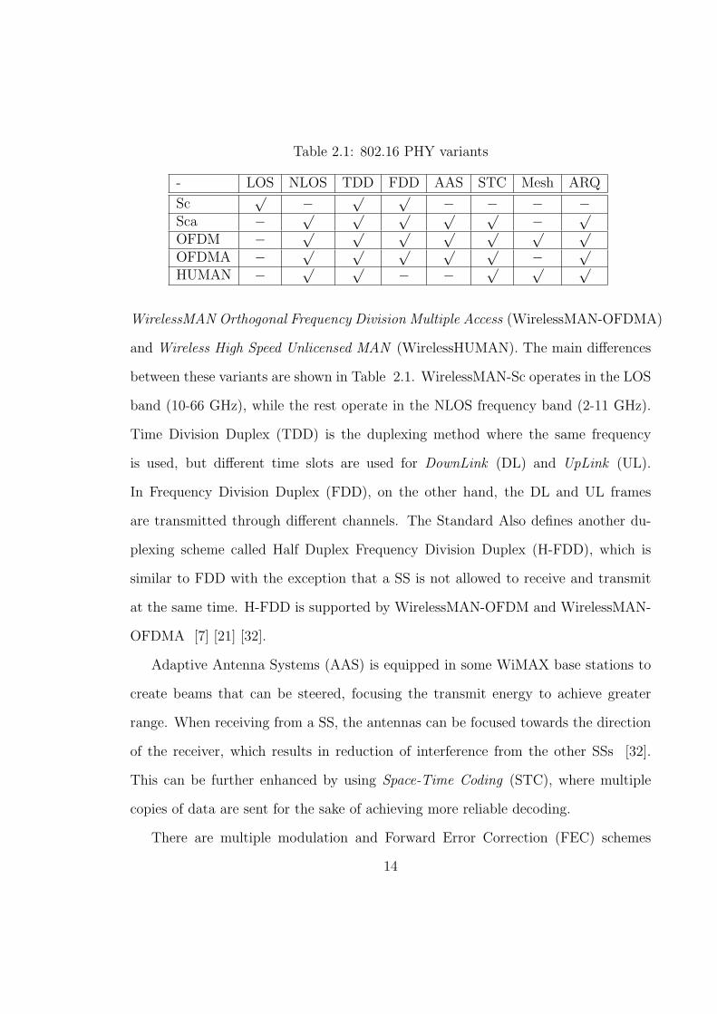
Table 2.1: 802.16 PHY variants

- LOS NLOS TDD FDD AAS STC Mesh ARQ

Sc√ − √ √ − − − −

Sca − √ √ √ √ √ − √

OFDM − √ √ √ √ √ √ √

OFDMA − √ √ √ √ √ − √

HUMAN − √ √ − − √ √ √

WirelessMAN Orthogonal Frequency Division Multiple Access (WirelessMAN-OFDMA)

and Wireless High Speed Unlicensed MAN (WirelessHUMAN). The main differences

between these variants are shown in Table 2.1. WirelessMAN-Sc operates in the LOS

band (10-66 GHz), while the rest operate in the NLOS frequency band (2-11 GHz).

Time Division Duplex (TDD) is the duplexing method where the same frequency

is used, but different time slots are used for DownLink (DL) and UpLink (UL).

In Frequency Division Duplex (FDD), on the other hand, the DL and UL frames

are transmitted through different channels. The Standard Also defines another du-

plexing scheme called Half Duplex Frequency Division Duplex (H-FDD), which is

similar to FDD with the exception that a SS is not allowed to receive and transmit

at the same time. H-FDD is supported by WirelessMAN-OFDM and WirelessMAN-

OFDMA [7] [21] [32].

Adaptive Antenna Systems (AAS) is equipped in some WiMAX base stations to

create beams that can be steered, focusing the transmit energy to achieve greater

range. When receiving from a SS, the antennas can be focused towards the direction

of the receiver, which results in reduction of interference from the other SSs [32].

This can be further enhanced by using Space-Time Coding (STC), where multiple

copies of data are sent for the sake of achieving more reliable decoding.

There are multiple modulation and Forward Error Correction (FEC) schemes

14

supported by WiMax. By utilizing Adaptive Modulation and Coding (AMC), WiMax

allows changing between these schemes based on channel conditions, and on a per

user or per frame basis. The supported schemes associated with their coding rates

are shown in Table 2.2.

Table 2.2: WiMax Modulation Schemes

Modulation Coding Rate Signal to Noise Ratiobits/symbol (SNR)

BPSK 0.5 6.4QPSK(1/2) 1 9.4QPSK(3/4) 1.5 11.216QAM(1/2) 2 16.415QAM(3/4) 3 18.264QAM(2/3) 4 22.764QAM(3/4) 4.5 24.4

The WiMAX MAC layer interfaces the physical layer with the upper network and

transport layers. The upper layers Service Data Units (SDU) are encapsulated in a

MAC PDU, which takes different formats depending on the size of the SDUs. If all

SDUs are of the same size, then they can be aggregated into the same burst to save

PHY overhead. For variable sized SDUs, the WiMax MAC layer supports flexible

allocation within the same MAC PDU to save MAC overhead. Conversely, if an SDU

is too large, it can be fragmented into multiple PDUs [7], see Figure 2.3.

In the PMP mode, the BS is completely responsible for allocating bandwidth

amongst subscriber stations. Similarly, most of the scheduling functionalities be-

tween the uplink and downlink traffic is done by the BS. For the downlink, the BS

allocates bandwidth based on the needs of the incoming traffic, while for the uplink it

is performed considering the SS requests. Before any data transmission, the BS and

SS establishes a unidirectional logical link, called a connection. Packets transmitted

15

MAC Header Subheaders (Optional) Paylod (Optional) CRC (Optional)

Packet Fixed Size MSDU

Packet Fixed Size MSDU

Packet Fixed Size MSDU

Packet Fixed Size MSDU

............. Packet Fixed Size MSDU

MAC PDU carrying several fixed length MSDUs

Packing subheader

Variable Size MSDU

Packing subheader

Variable Size MSDU

Packing subheader

Variable Size MSDU

.....

MAC PDU carrying several variable length MSDUs

Fragmentation Header MSDU Fragment

MAC PDU carrying a single fragmented MSDU

Figure 2.3: IEEE 802.16 MAC PDU Format

through that link use a common identifer called a connection identifier (CID), which

is the first of two addressing mechanisms. The second mechanism uses the concept of

a service flow, where packets sharing particular QoS parameters are identified through

a common service flow identifier(SFID). The QoS scheduling classes defined by the

IEEE 802.16d standard are Unsolicited Grant Service (UGS), Real-Time Polling Ser-

vice (rtPS), Non-Real-Time Polling Service (nrtPS) and Best-Effort (BE) service [2].

In the IEEE 802.16e, another service is added which is Extended Real-Time Polling

Service (ertPS). Table 2.3 shows the QoS parameters for each of these five classes

with an example of supported applications [7] [20].

2.1.2 WiMax Mesh Mode

In Mesh Mode nodes are placed in an ad hoc manner and can be viewed in two

different topological perspectives. In the first perspective, we can view the network

topology as a tree rooted at the BS and spanned to multi-levels with a random number

16

Table 2.3: QoS Services supported by WiMax

QoS Service QoS Parameters Application Example

UGS MSR, MLT, JT VoIP without silence suppressionrtPS mRR, MSR, MLT, TP audio/video streamingnrtPS mRR, MSR, TP FTPBE MSR, TP web browsing

ertPS mRR, MSR, MLT, JT, TP VoIP with silence suppressionMSR: Maximum Sustained Rate , MLT: Maximum Latency Tolerance

mSR: minimum Sustained Rate , mRR: minimum Reserved RateJT : Jitter Tolerance , TP : Traffic Priority

of nodes. In this setup, all communication is centrally controlled by the BS, which

determines all bandwidth allocations for nodes in all levels. Nodes in the first level

can communicate directly with the BS, while communication with nodes in further

levels is relayed by the intermediate nodes to and from the BS. The node used by

lower nodes as a relay for their data to/from the BS is called a Sponsor Node. It is

noticed from this that traffic generated by a node constitutes its own traffic added

to the traffic generated by all its sponsored nodes. Finally, communication between

nodes is limited to the sponsor(ed) relationship described above.

In the second perspective, we can view the network as a pool of clusters con-

taining multiple neighbor nodes. Every node, including the BS, establishes a logical

neighboring relationship with some of its neighboring nodes, such that every logical

neighbor is also a physical neighbor, while the opposite is not necessarily true. For a

node, a cluster is defined to include all nodes with which it has to coordinate before

performing any communication. The communication is done in a distributed fashion,

where nodes that are two-hops away contend for channel access, through an algorithm

called the election algorithm, described in Section 2.3.2. We notice that this access

method is used for the intranet traffic, in contrast to the centralized method which

17

is used for internet traffic.

When a new node decides to join the Mesh Network, it first scans for active net-

works and tries to establish coarse synchronization with the selected network. This

can be done through listening to the periodic broadcasted Mesh Network Configura-

tion (MSH-NCFG) messages, where parameters related to the PHY timing can be

extracted. Once the coarse synchronization is established, the node listens for further

MSH-NCFG messages and extracts the MAC parameters and slowly builds a list of

the physical neighboring nodes. The node then selects a candidate sponsor node, with

which it negotiates the basic capabilities and seeks authorization. The authorization

process involves verifying the security certificates, and determining whether the node

is eligible to join the network. Once authorization is approved, the candidate node

performs registration with the BS through the sponsoring node, and exchanges all

the necessarily parameters. Finally, the node can then communicate with its adja-

cent nodes to join the neighborhood.

Out of the five PHY variants, the WiMax mesh mode supports only two vari-

ants: WirelessMAN-OFDM and WirelessHUMAN, and the method used for regu-

lating channel access is TDMA. The frame structure consists of control and data

portions. Both portions are shared by the centralized and distributed schedulers. In

the control subframe, nodes declare their bandwidth requests, either through time

slots assigned by the BS, or through winning the distributed election algorithm. All

scheduling is done per link, without enforcing a distinction between uplink and down-

link traffic. QoS provisioning is performed per packet basis, and the end-to-end QoS

guarantee can be achieved through the centralized scheduler. Out of the long specifi-

cations of WiMax, in this chapter we focus our attention on the specifications of the

18

mesh frame structure and the functionalities of the schedulers, since they are related

to our contribution in Chapter 3. The following two sections will present the required

details on these two topics.

2.2 Frame Structure in WiMax Mesh Mode

The objective of our work is to find a partitioning scheme that would maximize the

utilization of the WiMax mesh frame. The description of the mesh frame, which we

present here, is the main technical background that relates to our work. The structure

and the configuration parameters will be extensively used later in Chapters 3 and 4.

All details provided in the following paragraphs bind to the description provided in

the 802.16d standard [2].

The IEEE 802.16 mesh mode uses Time Division Multiple Access (TDMA) for

regulating channel access among different nodes. The radio channel is divided into

frames, which are further divided into time slots that can be assigned to the different

nodes. The standard defines the allowed frame durations as indicated by Table 2.4.

The parameter that configures the frame length is called Frame Length Code and

appears in the Network Descriptor IE 1.

Every mesh frame is composed of two integral subframes: the Control Subframe

and Data Subframe, as shown in Figure 2.4. The control subframe carries configura-

tion messages that control the network cohesion and coordinated scheduling. On the

other hand, the data subframe carries the transmission bursts from different nodes in

the network. The following subsections give more insight into the structure of each

1The Network Descriptor Information ELement (ND-IE) is an embedded data carried by themesh configuration message (MSH-NCFG) used for updating subscriber stations of the channel andframe parameters.

19

Table 2.4: Frame Duration

Code Frame duration Frames Symbols per Frame(ms) per second (symbol duration = 12.5us)

0 2.5 400 2001 4 250 3202 5 200 4003 8 125 6404 10 100 8005 12.5 80 10006 20 50 1600

7-255 reserved - -

subframe.

2.2.1 Control subframe

The control subframe has two main objectives. The first is to create and maintain

cohesion between the various entities of the network. This is achieved by exchang-

ing configuration messages such as the Mesh Network Configuration message (MSH-

NCFG) and the Mesh Network Entry message (MSH-NENT). We term a frame that

carries cohesion control messages as a Network Control frame. The second objec-

tive is to coordinate the scheduling of data transfers amongst the various network

entities, which include the base station (BS) and the subscriber stations (SSs). The

message that carries such information is called a Mesh Centralized Scheduling Mes-

sage (MSH-CSCH). A frame that carries MSH-CSCH messages is termed Schedule

Control frame.

The Network Control frames occur periodically, as indicated by the Scheduling

Frames parameter in the Network Descriptor. Scheduling Frames parameter is defined

as the number of schedule control frames that occur between two consecutive network

20

Figure 2.4: Mesh mode frame structure

control frames. It is assigned values in multiples of four, with a minimum value of 0

and a maximum of 64. This is illustrated in Figure 2.5.

The length of the control subframe, regardless of its type, is fixed and equals

MSH-CTRL-LEN × 7 OFDM symbols. The MSH-CTRL-LEN parameter is defined

in the Network Descriptor with boundaries between 0 and 15. The network control

frame carries two types of configuration messages. The first is the Mesh Network

Entry (MSH-NENT) message, which provides the means for a new node to gain

synchronization and initial entry into a Mesh network. The MSH-NENT message

always appears in the first seven symbols of the network control subframe. The rest

of the MSH-CTRL-LEN −1 sets of seven symbols are used for network configuration,

21

Figure 2.5: Scheduling network control frames

through the Mesh Network Configuration MSH-NCFG. The specifications of MSH-

NCFG will be provided in sections 2.3.1 and 2.3.2.

The schedule control is designed to coordinate the scheduling among the different

entities. This includes scheduling in its two forms: centralized and distributed. There

are three main messages carried in the schedule subframe, namely Mesh Centralized

Schedule (MSH-CSCH), Mesh Centralized Schedule Configuration (MSH-CSCF), and

Mesh Distributed Scheduling (MSH-DSCH). The partition of the schedule control sub-

frame between the centralized and distributed schedulers is determined through the

MSH-DSCH-NUM parameter in the Network Descriptor. [(MSH CTRL LEN) −

(MSH DSCH NUM)]×7 symbols are allocated for the centralized and the rest are

assigned to the distributed.

The structure of every transmission opportunity in the control subframe starts

22

Figure 2.6: Structure of Control Subframe

by a long Preamble, then the MAC PDU with a specific control message, and finally

one or more guard symbols. Figure 2.6 provides an illustrative view for the different

structures that can appear in the control subframe.

Finally, it is worth mentioning that all transmissions in the control subframe are

sent using the QPSK − 1/2 modulation over the broadcast channel.

2.2.2 Data Subframe

The data subframe is located after the control subframe. It is divided into minis-

lots. The size of every minislot , with the possible exception of the last minislot, is

calculated using the following equation:⌈

OFDM Symbols Per Frame− 7 × (MSH − CTRL− LEN)

256

⌉

(2.1)

23

Every data minislot carries the physical transmission bursts from the BS and different

SSs. The coding and modulation schemes determine the data rate attainable for

different minislots.

The data subframe is also shared between the centralized and distributed sched-

ulers. This is determined by the MSH-CSCH-DATA-FRACTION parameter in the

Network Descriptor, which is defined as the maximum percentage (value × 6.67) of

minislots in the data subframe allocated for the centralized scheduler. The central-

ized portion of data always precedes the distributed one. The rest of the minislots

and possibly the minislots left unused by the centralized scheduler, are used by the

distributed scheduler.

2.3 Scheduling in WiMax Mesh Mode

As aforementioned, the IEEE 802.16 mesh mode supports two main schedulers: cen-

tralized and distributed. Each scheduler has two main operations, which are schedul-

ing the control messages and scheduling the data. The centralized scheduler is coordi-

nated between the BS and the various SSs for the transfer of the external traffic from

the Internet. On the other hand, the distributed scheduler is used to transfer intranet

traffic between nodes. There are two distinct types of distributed schedulers: coordi-

nated and uncoordinated. The following subsections will explore the functionalities

of these three schedulers.

24

2.3.1 Centralized Scheduling

The coordinated centralized scheduler is used for scheduling the data traffic transfers

between the BS and the SSs. This traffic is primarily external coming from the

Internet. The traffic can be in both directions: either downlink from the mesh BS to

the SSs, or uplink going from the SSs to the mesh BS. The base station (BS) is the

entity that coordinates this scheduling by determining how the SSs are to share the

channel in different time slots.

A distinct centralized scheduler is used for scheduling control messages and an-

other one is used for data. For the control scheduling, the objective is to inform every

node about its opportunity to transmit the MSH-CSCH and MSH-CSCF messages.

To achieve this, the BS calculates a global topology tree up to a pre-defined hop dis-

tance from the BS, and broadcasts it to the SSs. The tree information is embedded in

the Mesh Centralized Schedule Configuration message, MSH-CSCF. The one hop dis-

tant nodes from the BS will receive MSH-CSCF directly from the BS, and then relay

it down to the other nodes. This process repeats until the message is propagated to

the last node in the tree. The MSH-CSCF message carries the order by which nodes

shall abide in their transmission of the control messages. The order follows four main

rules:

Rule 1 The BS shall always transmits first

Rule 2 For every SS, the downlink shall always precede the uplink.

Rule 3 Nodes that are i hops away from the BS shall transmit before nodes that are

i+1 hops far from the BS

Rule 4 The node with a lower Node ID shall transmit first if both nodes are of equal

25

BS

SS1 SS2

SS3 SS4 SS5

Transmission Order: 1- BS to SS1 2- BS to SS2 3- SS1 to BS 4- SS2 to BS 5-SS1 to SS3 6-SS1 to SS4 7-SS3 to SS1 8-SS4 to SS1 9-SS2 to SS5

10- SS5 to SS2

Figure 2.7: Example of Centralized Scheduling

hop distance from the BS

An illustrative example is given in Figure 2.7. The BS is given the first opportunity

as indicated by Rule 1. Because of Rule 2 SS1 and SS2 receive from the BS before

transmitting. Since both SS1 and SS2 share the same hop distance from the BS,

then the node with the higher node ID, i.e. SS1, shall transmit before SS2. Similar

analysis can be applied to the other nodes.

Using the above control scheduling, every SS is given an opportunity to send

its MSH-CSCH request. All requests are sent to the BS, which will calculate the

26

uplink and downlink grants and send them to the different nodes through MSH-

CSCH grant messages. Using the grant messages, every SS will be able to determine

its schedule using a common algorithm that proportionally divides the frame to the

flow assignments [2].

The BS calculates the total number of slots for all SSs. If the sum of the slots

is less than or equal to MSH-CSCH-DATA-FRACTION, the data subframe can be

used directly. However, if the sum of requested slots is larger than MSH-CSCH-

DATA-FRACTION, then all reservations will be scaled down proportionally to fit in

one frame. If this results in infeasible allocations, two frames will be used. In this

process, the standard ensures fairness by ensuring that all active nodes gain a share

in every frame.

The centralized scheduler is relatively simple, because of the fact that all control

and data messages should go through the BS before taking any scheduling decision.

However, this increases the delay in the connection setup rendering the centralized

scheduler unsuitable for occasional traffic needs [13]. Another advantage of the

centralized scheduler is explicitly stated in the standard as: ”It is typically used in

a more optimal manner than distributed scheduling for traffic streams, which persist

over a duration that is greater than the cycle time to relay the new resource requests

and distribute the updated schedule” [2] [27].

There are many areas related to the centralized scheduling left undefined by the

standard. The main reason for this comes from one of the strengths of the 802.16

standard, which is flexibility. Vendors are given the freedom to specify and implement

these issues to the best of their needs and interests. A very clear example is that

although the standard has defined the messaging and control mechanisms, the way of

27

how slots are actually assigned to different nodes has not been defined [14] [38]. A

second example is the absence of a scheduling mechanism that would schedule control

messages, if the number of nodes in the mesh network is more than the available

slots for the centralized control messages. Another example, is the lack of a routing

algorithm that finds the optimum path from the many mesh routes between the BS

and the different SSs [26]. A final example is the scenario where a node is granted less

than its own and forwarding request. The standard does not specify how to divide

the grant between the actual request and relay requests [6].

There are various issues with the centralized scheduler which motivated many

researchers. Amongst these issues is the usage of a single connection at a time,

without any spatial reuse [26]. The lack of QoS validity is another issue, which did

not receive much attention so far [48]. In [6], eleven issues have been highlighted

related to the centralized scheduling, among which is the ordering delay, which arises

in a scenarios where a node sends before it receives. In such a common scenario, the

received data would have to be delayed to the next schedule opportunity.

2.3.2 Coordinated Distributed Scheduling

The coordinated distributed scheduler is one of the main mechanisms that feature the

mesh extension of the WiMax standard. It is mainly designed to schedule the intranet

traffic among different nodes. All nodes, including the BS, are treated equally, and

they contend for transmission opportunities. Every node coordinates its scheduling

with its extended two-hop neighborhood. It is clear from this that spatial reuse is

enhanced, allowing different neighborhoods to utilize the frame according to their

needs.

28

By explaining the distributed scheduler from a top-down approach, we can say

that the mesh network consists of a BS and multiple SSs. Different nodes create links

amongst each other forming different neighborhoods. For a node, a Neighborhood is

defined as all nodes that are within one or two-hops distance from it. All nodes within

a neighborhood compete for opportunities to send the MSH-DSCH messages in the

control subframe. This is achieved by all nodes running a global common algorithm,

called the election algorithm. Global means that all nodes run the same algorithm

and common means that when all nodes run it independently, it will yield the same

output. Similar to the centralized scheduler, data scheduling is determined from the

control messages; however, in a distributed manner in this case.

From the node’s perspective, when a node transmits, it determines its next trans-

mission time. However, since, the next proposed time can also be used by other

nodes, the node will contend for it. The node will run the election algorithm and if it

wins, it will broadcast its schedule to its neighbors. However, if it fails, it will choose

the next time slots and it will contend for it. This will be repeated until the node

wins. To ensure that every node wins the election algorithm in some period of time,

every node should backoff after transmission for a specific period of time without

performing any transmissions.

The MSH-DSCH message has two important parameters: XmtHoldOffExponent

and NextXmtMx. Whenever a node transmits, MSH-DSCH, it does not only transmit

its own parameters, but it also relays its neighbors’ parameters. Both parameters

are used to define two intervals: the eligibility Interval and Backoff Interval. The

eligibility interval is the interval in which a node is allowed to transmit, while the

backoff interval is the period in which that the node is not allowed to transmit. The

29

length of the eligibility interval is 2XmtHoldoffExponent. The actual transmission range

can be found from the following equation:

2XmtHoldoffExponent.(NextXmtMx) < NextXmtT ime ≤

2XmtHoldoffExponent.(NextXmtMx+ 1) (2.2)

After the eligibility interval, the node will backoff for at least 2XmtHoldoffExponent+4

transmission opportunities. After that the node calculates the earliest time it will

be eligible to transmit at (Earliest Subsequent Xmt Time) after the NextXmtTime,

which is calculated as: 2XmtHoldoffExponenet.NextXmtT ime.

The standard presented the specifications of the election algorithm. A node will

set the first slot after the backoff period as the candidate for the next transmission

opportunity. The node will have to compete with three types of nodes for this slot:

1. Nodes which have this slot located in its NextXmtT ime eligibility interval

2. Nodes which have this slot at or before its EarliestSubsequentXmtT ime

3. Nodes with unknown schedule.

The election algorithm is a pseudo-random function which takes as an input the

slot number and the nodes IDs. The output is a series of pseudo-random values.

If the maximum value is equal to the node ID, then it is considered the winner of

the algorithm, where it broadcasts its MSH-DSCH to the neighbors. The standard

defines a three-way handshake for connections between nodes. First, the node sends a

MSH-DSCH request. The destination node replies with a MSH-DSCH grant. Finally,

the requesting node confirms this by broadcasting a MSH-DSCH message with a copy

of the granted slots.

30

Issues related to the coordinated distributed scheduler can be found in [6] [9] [13] [38].

One of the issues is the fact that all nodes compete periodically in the election al-

gorithm whether they have data to send or not. The standard also does not define

a limit on the maximum number of slots that a node can seize when it wins the

election algorithm. With the current specifications, a node can monopolize the whole

distributed scheduling portion of the frame at the moment it wins the election algo-

rithm. Finally, scalability is a major concern, as the performance of the scheduler

would sternly degrade in dense mesh networks.

2.3.3 Uncoordinated Distributed Scheduling

As the name implies, the uncoordinated scheduler allows nodes to compete for time

slots without any prior coordination. It is designed for fast and ad hoc setups of

schedules on a link by link basis [2]. The uncoordinated distributed scheduler is

similar to the coordinated scheduler in the three-way handshake process mentioned

in the previous section. It also uses the mesh distributed message, MSH-DSCH, with

the difference that the Coordination Flag parameter is set. The mesh frame structure

does not reserve any control time slots for the uncoordinated schedule. Thus the

uncoordinated MSH-DSCH messages can only occur in the data subsection. Unused

data slots in both the centralized and the distributed schedulers are liable to the use

of the uncoordinated scheduler.

The standard has not provided a specific uncoordinated scheduler, allowing im-

plementation freedom to different network vendors and service providers. The only

condition stated by the standard is that the uncoordinated data should not collide

31

with the coordinated control and data traffic. The main drawback of the uncoor-

dinated scheduler is the unreliability, allowing collisions to take place. In [6], it

has been argued that this, along with the standard limitation of not colliding with

other schedulers, and the previous extensive attention to the contention-based access

schemes are the main reasons for not receiving a dedicated research interest in this

type of schedulers.

2.4 Related Work

In the recent WiMax publications, there is no published algorithm for partitioning

the WiMax mesh mode frame. Works related to WiMax mesh scheduling, in both

modes: centralized and distributed, are the closest research areas to our work. In

addition, some of the works on QoS in TDMA networks, WiMax traffic modeling,

and PMP frame partitioning are partially related to this work.

In [48] [49], the authors presented some centralized scheduling algorithms through

developing a finite horizon dynamic programming framework which optimizes a cost

function over a fixed number of time slots. Using the cost functions, and after fixing

the routing in the network, the optimum scheduling scheme is chosen. Amongst the

studied schemes are Maximum Transmission, Per Slot Maximum Transmission and

Adaptive Fixed Allocation. However, the schemes can only be applied to uplink

scheduling, and no method for partitioning the frame between uplink and downlink

was proposed [6].

In [13], the performance of WiMax mesh coordinated distributed scheduler is

studied. The authors mainly targeted the relationship between contention −winning

32

the election algorithm− and total number of nodes, network topology and the expo-

nent value. When increasing the total number of neighbors or the exponent value, the

backoff periods increase, affecting the performance of the system. It has been high-

lighted in the paper, however, that the exponent value has a more significant impact.

Finally, the authors suggested using small exponent values for nodes with real-time

traffic. In [53], the authors raised the observation that coordinated distributed mes-

sages can collide in the extended neighborhoods, which has been ignored by previous

performance studies. The performance of the scheduler was studied under a realistic

interference model. It has been shown that the contention ratio increases to 20%

for 2-hop extended neighborhood and to 7% for 3-hops. The authors suggested cer-

tain configurations for the election algorithm parameters to avoid such performance

degradation.

In [22] and later in [23], the authors studied the frame of TDMA networks, but

for the objective of finding the minimum number of slots required to supported a

requested guaranteed QoS in the network. The QoS is defined in terms of both delay

and bandwidth, and specifically VoIP traffic was studied. The optimization problem

for finding the minimum number slots was built on the TDMA propagation delay

(TDMA round trip). This work is the closest to this study in terms of finding the

allocation in a frame that includes centralized and distributed schedulers. However,

the objectives differ in that they target finding the minimum partitioning for sup-

porting a specific QoS requirement, while we target finding the best partitioning for

the network so that to maximize utilization and support multiple traffic classes.

The study in [6] provided the inspiration for our work. The authors studied the

mesh schedulers, both centralized and distributed, and provided thorough reviews

33

of the current work in WiMax mesh scheduling. Issues with the both schedulers as

defined by the standard were presented. In the centralized scheduler, the lack of

spatial reuse, routing algorithms, QoS support and multiple channels support were

highlighted. The issue of frame partitioning and utilization was explicitly mentioned

as one of the open issues, which is the core of this study. For the distributed sched-

uler, issues like the effect of holdoff time, faireness, handshake priorities, QoS and

scalability were discussed.

There are some recent proposals for frame partitioning and dynamic bandwidth

allocations for the PMP mode [17] [44] [47] [36]. The problem of partitioning the

PMP frame is different than that of the mesh frame in two main aspects. The first

difference comes from the fact that the PMP frame partitioning is a problem of finding

the appropriate ratio between the uplink and downlink allocations, while in the mesh

mode allocations are done per link regardless of being uplink or downlink. Whenever

uplink and downlink partitions are used, asymmetric approaches are preferred as SS

tend to download more than to upload. However, assigning low allocations for the

uplink will result in low performance for the TCP traffic [17]. The second difference

comes from scheduling and the method of how different nodes are assigned their

bandwidth allocations. In the PMP mode, all allocations are centrally controlled by

the BS, while in the mesh mode the scheduling is achieved in both centralized and

distributed manner. Amongst the WiMax variants, the 802.16j frame structure is

expected to be the closest to the mesh frame structure. There are some proposals

for the 802.16j frame structure [18] [51], however, the document is still under the

draft stage and these proposals are still under discussion and they require further

performance evaluations.

34

Chapter 3

Frame Partitioning in WiMax

Mesh Mode

3.1 Problem Description

As previously mentioned, the WiMax mesh mode frame structure is composed of two

main parts: control and data, which is further divided into centralized and distributed

as shown in Figures 2.4 and 2.6. The 802.16 standard allows variable partitioning

between the control and data subframes, and further internal partitioning between

the two schedulers. Nevertheless, the standard provides no specific scheme for such

partitioning. We argue that imposing a carefully designed partitioning scheme would

maximize the utilization of the frame, and would certainly reflect on improving the

QoS performance of the system.

In this work, we aim at proposing such a partitioning scheme, by studying the

long and short run behavior of the system and predicting an efficient partitioning to

increase the utilization of future frames. We use a Markovian model, in which the

35

system is represented by states, where every state represent the number of occupied

symbols. Using this method we study the system behavior over a large (coarse)

window and then provide a prediction from the stationary distribution of the Markov

chain. This partitioning is then fine tuned by a statistical analysis of small (fine)

window to adapt to the recent changes of the data traffic.

Let us assume that the size of the Data Subframe is LD symbols, where the size

of the centralized portion is LDC symbols and the size of the distributed portion is

LDD symbols, such that:

LD = LDC + LDD (3.1)

Let us also assume that the possible values for LDC and LDD are in the range

[LDmin, LDmax]. Our problem is to find the optimal values for LDC and LDD in

the given range that would maximize the frame utilization. We achieve this by con-

ducting statistical analysis of the system in coarse and fine windows. For the coarse

window, we use the stationary distribution of the long-run behavior of the Demand

Markov chain D which deduces the optimum partitioning in the long run. For the fine

window, we use statistics represented by the probability matrix C (current demand),

to tune the long run partitioning to the current changes in the traffic.

There are two main factors that control how frame utilization can be measured.

The first is to measure how much data (bits) are carried by every symbol, and then

sum the total bits transmitted in a frame. The second method is to count the number

of symbols that carry some data (non-empty symbols). In the context of this thesis,

we exclusively use the second measurement method for frame utilization. This choice

comes from the fact that the amount of data transmitted in every symbol is controlled

by the channel quality of different links, which is an external factor to the system.

36

Channel quality is affected by factors such as weather, obstacles or mobility, which

are beyond the control of the system. Therefore, when we say that our objective

is to increase the frame utilization, we refer to trying to decrease the number of

empty symbols. If a scheduler is given a large portion of the data subframe, then the

probability of having empty symbols is increased. On the other hand, if the scheduler

is assigned a small portion of the data subframe, then this may be not enough to satisfy

the demand of different nodes, and may consequently result in packet overflow. The

optimum goal of our scheme is to partition the data subframe such that the number

of empty symbols approaches zero, which implies a full utilization.

3.2 System Model

The system model that we propose here is designed taking into consideration three

objectives. The first is to abide to the specifications of the 802.16d standard, and

impose no changes to any of the specifications. The second is to consider practical as-

sumptions that would ensure the viability of our scheme. Finally, the model is mainly

designed to show the effect of frame partitioning on the overall system performance.

Therefore, parameters that have minimum or absent effects on the frame utilization

will be assumed fixed at reasonable values.

Starting with the schedulers, we assume that both the centralized and distributed

schedulers are active at all times. This assumption implies that the system should

not allow one of the schedulers to monopolize the data subframe. Therefore, at any

given moment, the size of both LDC and LDD is greater than or equal to a certain

non-zero threshold, which we denote as LDmin. Large values of LDmin decrease the

utilization of the frame, while very small values might cause un-satisfaction to to the

37

demand of the other scheduler.

We give higher priority to the centralized scheduler over the coordinated dis-

tributed scheduler. We argue that it is better to have more free symbols in the

centralized portion of the data subframe, than that of the the distributed sched-

uler. The reason lies in the fact that the distributed scheduler can always use the

empty symbols of the centralized through either the coordinated or uncoordinated

distributed schedulers. On the other hand, the centralized scheduler can not use any

of the empty distributed symbols. Also, due to the TDMA nature of the frame, the

centralized portion comes before the distributed portion. Therefore, the distributed

scheduler can always check the unused symbols in the centralized portion, but the

reverse is not practically possible. Building on these two reasons, our proposed algo-

rithm bases its decision on the data collected from the centralized scheduler and not

the distributed one.

The proposed scheme is generic and is supposed to work under different imple-

mentations of centralized data schedulers. Also the scheme is independent of Call

Admission Control (CAC) schemes, as we assume that connections are already ad-

mitted into the system and are fed to the scheduler. Without loss of generality, we will

use the centralized data scheduler defined by the standard, as explained in Section

2.3.1.

The input to the scheduler is the traffic received from the admitted connections.

The scheduler evaluates the incoming bandwidth requests specified in the centralized

portion of the control subframe and outputs the symbol allocation for every node.

Since the uncoordinated scheduler is contention-based and does not affect the per-

formance of both coordinated schedulers, we consider that is not implemented. The

38

importance of this assumption comes from the fact that we would like to measure

the frame utilization based on decisions taken by the coordinated schedulers. The

uncoordinated scheduler will always increase the utilization of the frame, and its ab-

sence will enable us to measure more accurately the effect of our proposed algorithm

on the frame utilization. Finally, the control schedulers are used according to the

specifications provided by the standard as described in Section 2.3.

The frame duration can be set to any of the values defined in Table 2.4, which will

reflect on the number of symbols available at every data subframe. The scheduling

frames parameter in the Network Descriptor can be set to any value in multiple of

fours (0-64). The only restriction we impose is using fixed values for the the frame

parameters along the run time of the partitioning algorithm. If any of these values

is to be changed, then the BS will need to re-broadcast the new values and all SS

should re-synchronize, and hence the algorithm should be restarted. In other words,

the partitioning algorithm is generic to frame duration.

3.2.1 Network Model

We use the standard WiMax network model, where there is only one BS in the

network and multiple Subscriber Stations (SS) connected to it. We treat all SS

equally regardless of the number of hosts connected to the individual units. We

assume that every node will have a guaranteed chance to send its bandwidth request

in the centralized portion of the control subframe for every frame. The reason behind

this assumption is that the standard does not specify a scheduler when the number

of nodes is larger than the available control slots. We remark that designing such

a scheduler is beyond the scope of our work. Nevertheless, controlling the size of

39

the centralized control partition can be done through tuning the value of the MSH-

DSCH-NUM parameter in the Network Descriptor, which we will assign a fixed value.

The topology should be created in such a way as to reflect the benefits of the mesh

network. Hence, we assume that the network has at least one node that is two hops

far from the BS. We also assume that at least half of the number of nodes are not

connected directly to the BS.

Ideally, the size of every neighborhood should be reasonable and sensitive to the

MSH-DSCH-NUM parameter. A threshold for the minimum probability of success in

the election algorithm should be maintained in all neighborhoods. Therefore, during

the process of choosing a sponsor, the sponsor node should reject any new node if it

will result in decreasing the success probability beyond the permitted threshold. Find-

ing this probability is a difficult problem, as it depends on many parameters which

are network dependant. For example, the network topology affects how the neigh-

borhoods are formed, and thus creates regions with different success probabilities.

Further discussion about how this probability can be calculated and the difficulties

associated with it can be found in [13].

An example of a network that binds to the above assumptions is illustrated in

Figure 3.1.

3.2.2 Bandwidth Requests

Subscriber stations in WiMax networks work as a backhaul, gathering aggregate

requests of multiple hosts. Hence, it is practical to assume that the base station

always receives requests, meaning the sum of SS requests is always non-zero. This

assumption meets with the standard specifications, where a node, whenever granted

40

Number of BS = 1 Number of SS = 14 Tree Depth =3 Nodes connected to BS = 4 (30%) Max# Neighbors = 5

Base Station

SS# 1

SS# 5

SS# 8

SS# 9

SS# 2

SS# 13 SS# 12 SS# 14

SS# 10 SS# 6 SS# 7

SS# 3 SS# 4

Figure 3.1: Example of WiMax mesh network

a chance to request, will request a small number of symbols to maintain its reserved

slots for future usage [2].

We also assume that there is a limit on the number of symbols that a node

can request per frame [15]. This is important for two reasons. The first is to

maintain fairness between nodes, and prevent aggressive nodes from monopolizing

the frame. The second is the limited size of the frame, where its size can not be

extended indefinitely. The standard suggests two procedures for dealing with the

scenario where the number of requested symbols is more than the available symbols.

41

The first is to scale down all requests proportionally, and the second is to use an

extended frame which equals the size of two frames [2]. In both cases, however,

there is a limit where the BS has to trim down the requests to fit in the available

symbols. For the above reasons, we assume that whenever a node makes a bandwidth

request, it does not request more than λmax symbols. This value depends on multiple

parameters such as the number of nodes in the network, the topology and frame

duration. Further discussion about this value will be addressed in Section 4.1.2.

From the implementation perspective, nodes can be either explicitly informed about

the value of λmax, using some of the reserved bits in the MSH-NCFG message, or

when the BS trims down the extra requested symbols before scheduling the traffic.

The method of scaling, as described by the standard, will be applied in our scheme.

However, whenever the scheduling process results in using two frames instead of one,

we will deal with the two frames as a single long frame, to simplify statistical data

collection and analysis.

The SS request λni starts in the SS itself, where it checks its queues and calculates

the number of bytes to request. This value is embedded in the MSH-CSCH message,

and is sent either directly to the BS, or if not directly connected to the BS, by the

relaying parent nodes. The BS receives this request and converts it to symbols using

the sensed channel quality. The BS gathers all requested symbols by different nodes

and use a data scheduler to specify how many symbols are allocated for every node

and the portion of the data subframe where this allocation is assigned. Henceforth,

whenever we use the term demand, we refer to this allocation of symbols as an output

of the data scheduler, and not the actual bits request. In the special case when the

scheduled demand exceeds the available symbols, the BS will perform the necessary

42

scaling to fit the demand in a frame. It has been noted in [6] that when a node receives

its allocation, the BS does not specify how to divide the allocation amongst the parent

and child nodes. We assume here that the allocations are divided proportionally to

the requested traffic, to ensure fairness among nodes.

3.3 Mathematical Model

3.3.1 Preliminaries

The objective of the proposed partitioning scheme is to predict the best partitioning

for the data subframe between the centralized and distributed schedulers, based on

the current and previous behavior of the network.

The algorithm has two main phases. In the first phase, we predict the best par-

titioning based on statistics gathered on a previous large window, which we call a

Coarse Window. On the other hand, the second phase tries to adjust the suggested

partitioning of the coarse window to accommodate the small scale changes of the

traffic. This is based on statistics gathered in a small window, which we call a Fine

Window. The predicted partitioning by the first phase is only applied at the end of

every coarse window. However, the second phase can be considered real-time, as it

can be applied, if necessary at the end of every fine window. A high level graphical

illustration about the partitioning approach is depicted in Figure 3.2.

Since the physical layer of the mesh mode uses HUMAN (OFDM/TDMA), we will

use the OFDM symbol as our main unit. However, our scheme can allow different

granularities. We define the frame unit ψ as a group of OFDM symbols indicated by

the system granularity. The minimum value for ψ is one symbol and the maximum

43

Coarse Window i-1 Coarse Window i Coarse Window i+1

Fine Window j

- Data Scheduler Collect Node requests from

the control subframe - Outputs the symbols allocations in the data

subframe

Collect Statistics for Coarse Window (Markov Chain

Probability Matrix)

Collect Statistics for Fine Window

No

Start of Coarse Window

Start of Fine Window

End of Fine Window

End of Coarse Window

No

Yes

Yes

Frame Building

Fine Window Partitioning

Coarse Window Partitioning

Figure 3.2: Partitioning Algorithm Flow Chart

possible value is half of the number of symbols in the data subframe. For presentation

purposes, and unless otherwise stated, we will use the data mini-slot interchangeably

with ψ. This means that each ψ unit will have a number of symbols equal to the

number that can fit in a data-mini slot. As indicated in Section 2.2.2, number of

symbols in a data mini-slot depends on the frame duration code and the length of

the control subframe. The main effect of the value of ψ is the algorithm complexity,

as the computational complexity increases inversely with the value of ψ.

44

We use dual discrete quantization for the utilization of ψ. Meaning, ψ is either

utilized (ψ1) or empty (ψ0). Formally, we say that a unit ψ is utilized if at least one

of its symbols is non-empty. If all symbols are empty, ψ is then considered empty.

Using this definition, we can restate our objective as to design a partitioning algorithm

that would increase the number of ψ1 units. The following subsections present our

approach to achieve this goal, and describe in detail the two phases of the scheme.

3.3.2 Coarse Window

Size of Coarse Window

The coarse window is a large time window that contains many WiMax mesh frames.

The window should be large enough to collect statistics that characterize the long-run

behavior of the network. We know from Section 2.2.1 that the control subframe can

be either network or schedule control. Our interest here is on frames of the second

type. Therefore, the number of frames in a coarse window (Fc) is the total number

of schedule control frames, which can be calculated as the the total number of frames

subtracting the network control subframes, as indicated in Figure 3.3.

The time length of the coarse window depends on the frame duration. The number

of frames in a coarse window Ff is inversely proportional to frame duration. For higher

values of frame duration, the window time T should be expanded to allow enough

collection of statistics. Our simulations showed that a size of 1,600 frames or more

is necessary for acquiring stable results. Taking the extreme value (largest frame

duration = 20ms), a window size of no less than half a minute was large enough to

collect the necessarily statistics for all frame durations.

45

.

. T : Length of coarse window in milliseconds

. Ff : Number of frames in a coarse window (scheduling frames)

. FrameDuration: length of a frame in milliseconds

. SchedulingFrames: A parameter in the Network Descriptor representing number of

. scheduling frames between two consecutive control subframes

.

. Ff = TFrameDuration

− TSchedulingFrames

.

Figure 3.3: Calculation of window sizes

Demand Markov Chain

We use a discrete Markov chain (DMC) to model the possible frame occupancy, based

on the requested slots and the size of the centralized portion of the data subframe.

Every state represents the aggregate number of data symbols requested by all nodes

of the network in a frame. For example, if we say that the system is in state 100, it

means that the sum of the requests of all nodes that appears in the control subframe

is equal to 100 ψ units for a current frame frame. We denote our Markov chain as

D (standing for Demand). The number of states in the chain (DS) is equal to the

maximum possible value of ψ units that can be requested by all nodes for a frame,

which can be calculated according to the following equation:

DS =256 − LDmin

ψ(3.2)

A state i represents the actual requested number of ψ units, calculated as∑N

n=0 λni,

where N is the number of nodes in the network, and λni is number of units requested

by node n for frame i. This value does not represent the frame occupancy, but rather

the way that nodes would have expected the frame to be utilized. Taking an example

where in the coarse window j the value of LDC(j) is equal to 100, if all nodes request

46

80 units, the system would be considered in state 80, regardless of the wasted 20

units. Similarly, if all nodes request 120 units, the system would be considered in

state 120, although only 100 units will be assigned through the process of scaling.

The probability Matrix of the Markov chain (PD) is of size DS × DS, which is

sensitive to the system granularity ψ. PDi,jdonates the probability that the system

will transit to state j (i.e. request j ψ units), if the current requested ψ units is equal

to i.

At the beginning of every coarse window, all probabilities in the PD matrix are

initialized to zero. During the coarse window, counters are used to log the occurrence

of different events (i.e. transitions from one state to another). For example, if the

demand in the current frame is λi and the demand of the following frame is λi+1, then

the counter of Di,i+1 will be incremented. If the value of λi is more than LDmax, a

scaling will take place and the counter of D(i−1,LDmax) will be incremented. Similarly,

when the value of λi is less than LDmin the counter of D(i−1,LDmin) will be incremented.

At the end of coarse window, the probabilities are calculated by dividing every counter

by the sum of every row, which represents number of times a specific λ was requested.

In Figure 3.4, we show a simplified example of the demand Markov chain. We

assume that the size of the centralized portion of the data subframe is equal to 6

slots. Hence, the size of the Markov chain probability matrix is equal to 6 × 6. If we

start from state ”3 Slots”, it means that the sum of requested slots by the network for

the previous frame is equal to 3 time slots. The transition probabilities, illustrated

as arrows emerging from the state, represent the probabilities of the sum of requests

of the network by the following frame. For example, the probability that the network

requests 1 slot for the next frame equals to 0.1. Note that, in practice the size of

47

1 Slot 2 Slots 3 Slots

4 Slots 5 Slots 6 Slots

0 . 2 0 . 4 7

0 . 9 0 . 1 7

0.3

0 . 5

0 . 2 0.2

0.13

0 . 1

0 . 2

0 . 3

0 . 2

0 . 2

0 . 1 0 .

3 3

0 . 3 3 0 . 1 7

0 . 2

0 . 2

0 . 4 0 . 2

Data subframe size: L D

= 10 slots Centralized data size: L

DC = 6 slots

Distributed data size: L DD

= 4 slots

Markov Chain

Probability Matrix

20 . 0 40 . 0 20 . 0 20 . 0 00 . 0 00 . 0

00 . 0 90 . 0 10 . 0 00 . 0 00 . 0 00 . 0

00 . 0 20 . 0 20 . 0 30 . 0 20 . 0 10 . 0

13 . 0 00 . 0 20 . 0 47 . 0 00 . 0 20 . 0

00 . 0 00 . 0 50 . 0 30 . 0 20 . 0 00 . 0

= D

Figure 3.4: Demand Markov Chain

the markov chain is much larger, however; the size can be minimized by setting the

granularity ψ to higher values.

In Figure 3.5, we show an example of calculating the transition probabilities.

As previously mentioned, the probabilities are calculated empirically, by gathering

statistics about the demand in a coarse window. The example presented in the figure

is when the sum of requests for the first frame equals to 3, and the sum of requests for

the second frame equals to 4. In this case, the counter {3}{4} will be incremented,

48

Data subframe size: L D

= 10 slots Centralized data size: L

DC = 6 slots

Distributed data siz : L DD

= 4 slots Number of frames in coarse window = 100 frame

1 2 3 4 5 6 1 0 0 0 0 0 0 2 0 0 0 0 0 0 3 0 0 0 1 0 0 4 0 0 0 0 0 0 5 0 0 0 0 0 0 6 0 0 0 0 0 0 At the end of the coarse window, probabilities are calculated

1 2 3 4 5 6 Sum 1 0 2 3 5 0 0 10 2 3 0 7 3 0 2 15 3 2 4 6 4 4 0 20 4 0 0 0 1 9 0 1 0 5 0 10 0 10 5 5 30 6 0 0 1 1 2 1 5

Counters

1 2 3 4 5 6 1 0.00 0.20 0.30 0.50 0. 0 0 0.00 2 0.20 0. 0 0 0.47 0. 2 0 0.00 0 .13 3 0.10 0.20 0.30 0.20 0.20 0.00 4 0.00 0.00 0.00 0.10 0.90 0.00 5 0.00 0. 33 0. 00 0.33 0.17 0.17 6 0.00 0.00 0.20 0.20 0.40 0.20

Probabilities

Demand of Frame 1 = 3 Demand of Frame 2 = 4

Figure 3.5: Calculation of PD Matrix

indicating the occurrence of this event. At the end of the coarse window, all counters

are used to calculate the probabilities as shown in the bottom two tables.

When the probabilities are calculated at the end of the coarse window, the station-

ary distribution π of the Markov chain is computed. Since the stationary distribution

represents the portion of time the system will be spending in that state, a reason-

able decision would be to assign the value of the centralized partition equal to the

maximum value in the stationary distribution.

From a theoretical perspective, the traffic generated by every node can be modeled

49

as a Poisson Process, which is a common model used for this type of traffic [46]

[10] [11] [42]. The Poisson processes of different nodes are independent of each other.

Since the sum of multiple independant Poisson Processes is also a Poisson process,

then at the BS the sum of all requests generated by all nodes is also a Poisson

Process with a rate equal to the sum of the rates of the different processes. The

random variable is the counter of the number of requested symbols, and the time is

the length of the coarse window. Using such a model, which is Markovian by nature,

is enough for guaranteeing the ergodicity of the chain, and hence the existence of a

stationary distribution [19].

System State

We define the system state as the tendency of the network traffic requests. If the

network tends to request high number of symbols, then we say that the network is

in High Demand. Similarly, if the network tends to request few number of symbols,

we say the network is in Low Demand state. Since, ”high” and ”low” are relative

terms, we formally define the system state as shown in Figure 3.6. For example, if

the stationary distribution π =[0.05 , 0.13 , 0.07 , 0.35 , 0.25 , 0.15], then the system

is considered in high demand, because (0.25+0.15) is larger than (0.05+0.13+0.07).

The system state will be used in the algorithm to make sure that the partitions

recommended by the fine window do not conflict with the coarse window partitions.

3.3.3 Fine Window

As the coarse window tries to choose the best partition that would maximize the

overall frame utilization, statistics from the fine window aim at adjusting the partition

50

. Let the stationary distribution of the system be π.

. Let the maximum value in π is πi

. Let d1 =∑i−1

j=0 πj and d2 =∑LDmax

j=i+1 πj

.. If d1 > d2

. Then state = Low Demand.

.. If d1 < d2

. Then state = High Demand.

.. else //d1 == d2

. Let k be the index of the next maximum value in π.

. If k < i

. Then state = Low Demand

. If k > i

. state = High Demand

. else if !End of π vector

. Repeat from line 10

. else

. state = High Demand

Figure 3.6: Network State

to changes in the demand. Changes in the demand can be either a result of a change

in the state of the network, as in the case new nodes join/leave the network, or the

result of a change in bandwidth requests for a specific service, like an increase in

the number of users watching a video streaming. Since these changes might cause

the over-utilization of the following frames, fine tuning the partition would allow the

system to efficiently respond to such changes.

The size of the fine window is much smaller than that of the coarse window.

Nevertheless, if we choose a very small window, the system would be responding to

short bursts of traffic rather than actual traffic changes, and probably not enough

statistics would be collected to reflect the demand behavior. From the other side,

the larger the fine window, the slower the system reaction to demand changes, which

51

is reflected in the degradation of the utilization. Our simulations showed that a fine

window size (Ff ) of 1%−5% of the coarse window was generally reasonable. However,

parameters such as the frame duration and the size of the coarse window should be

carefully taken into consideration before choosing the size of the fine window.

From the fine window we build two probability matrices. The first is the demand

matrix, which we denote as C and the second is the satisfaction matrix which we

denote as S. The C matrix is of size LDC

ψ× LDC

ψ. Since LDC is a configurable

parameter, the matrix C will have different sizes for different coarse windows. If the

demand is equal to LDC then it either means that:

1. The demand was precisely LDC , or

2. The demand was more than LDC and a scaling took place.

The first case means that the current partitioning meets exactly with the demand;

however, the second means that the current partitioning is less than the demand of the

system. To differentiate between these two scenarios, we create the second probability

matrix, which is the satisfaction matrix S. Our trigger for the satisfaction is scaling.

If no scaling takes place then the demand is satisfied, and the reverse is true. The size

of the satisfaction matrix is LDC × 2. The first column refers to satisfaction and the

second refers to dissatisfaction. Both matrices are computed as depicted in Figure

3.7.

At the beginning of every fine window, both C and S are initialized to zero.

Similar to the procedure of the coarse window, counters are used to log the occurrence

of different events. The main difference is that the counting takes place in the fine

window after applying the scheduling process, while in the coarse window the counting

is performed before. Let us assume that the current centralized size (LDC) equals 100

52

. Let the current demand be λi , ψ = 1,

. and the current data centralized size is LDC

.

. If !End of fine window

. If λi < LDC Then

. C(i−1,i) + +

. else if di == LDC Then

. C(i−1,LDC) + +

. S(i−1,1) + +

. else if di > LDC Then

. C(i−1,LDC) + +

. S(i−1,2) + +

.

. if End of fine window

. calculate probabilities

. ∀ i,j PC(i,j)=

C(i,j)∑LDC

i=0 C(i,j).. i = 1, 2:

. PS(i,1)=

S(i,1)

S(i,1)+S(i,2)and PS(i,2)

=S(i,2)

S(i,1)+S(i,2)

Figure 3.7: Calculation of PC and PS probability matrices

ψ units, and the previous scheduled number of symbols was λi−1 = 60. We have three

distinct scenarios depending on the value of current scheduled traffic λi. The first

scenario is when λi < LDC , (e.g., λi = 80) which implies that the frame is not fully

utilized. In this scenario only the counter C(60,80) is incremented and no counter is

incremented in the matrix S. The second scenario takes place when the value of λi is

exactly equal to LDC (100). The counter C(60,100) will be incremented, alongside S(60,1)

which represents the satisfaction (i.e. no scaling took place) of the system. Finally,

if λi is greater than the current available symbols (LDC), then a scaling would take

place and λi would have the value of LDC (100). In this scenario the counter C(60,100)

will be incremented, but this time S(60,1) will be incremented as well to demonstrate

53

the unsatisfaction of the system.

Both C and S help us determine if the partition applied by the coarse window

meets the expectation of the current traffic. The output of C and S can suggest an

increase or decrease of the value LDC . However, the suggested value of LDC by the

fine window is not necessarily adopted. Therefore, we can say that the coarse window

enforces partitions while the fine window recommends. The following subsection

describes how to use D, C and S to predict the best partitioning.

3.4 Prediction for optimal frame partitioning

3.4.1 Preliminaries

The main objective of this section is to combine the recommendations of both coarse

and fine windows to provide the system with the proper frame partitioning. At

the end of every coarse window, the frame will be re-partitioned such that LDC =

πmax. The system state will also be determined. At the end of the fine window, a

recommendation for partitioning will be proposed. We use the system state to resolve

any possible conflict between the two recommendations. If the state is high demand,

and an increase is requested by the fine window, then it should be applied. However,

if no increase is requested, then the partition is kept unchanged. From the other

angle, if the system state is low demand then we argue that all recommendations

by the fine window are to be neglected. This is based on our assumption that the

centralized scheduler has higher priority than the distributed, and it is better to have

free symbols in the centralized than to unsatisfy its demand.

The above description raises two important questions. The first is how does the

54

fine window determine if an increase is needed? The second, if an increase is to be

applied, then what is the value of that change?

To answer the first question, we take a careful look at the matrices C and S.

There are two scenarios that trigger the need for an increase.

Scenario 1 The highest probability in PC is PC(LDC ,LDC) and the probability of unsatisfac-

tion is higher than the probability of satisfaction, i.e. PS(LDC,1) < PS(LDC,2). This

means that there are many instances where the frame has been fully utilized,

and that was a result of the partition being unable to satisfy the demands.

Scenario 2 The overall probability of unsatisfaction is higher than probability of satisfac-

tion:∑LDC

i=1 PSi,1<

∑LDC

i=1 PSi,2, where the probabilities are calculated on enough

many events. Note that this is different than the first scenario as it does not

require the maximum demand to be equal to LDC .

If any of the above two scenarios apply, then we say that the fine window requests

for an increase. Otherwise, the fine window requests no change.

To answer the second question, we propose two ideas. The first is to use a fixed

number of symbols to be added to the current size of the centralized portion of data.

We call this method Frame Partitioning with Gradual Increase which we describe in

Section 3.4.2. The second is to increase to the second maximum value in the stationary

distribution. We call this method Frame Partitioning with Maximal Increase and we

describe it in Section 3.4.3. The first method is more appropriate when the values

of πi are close to each other, and the second method is more appropriate when the

values have high differences. In mathematical terms, when the variance of the values

in π is low then the first method is more appropriate, and when the variance is high

the second method is preferred.

55

Since there are multiple fine windows in a coarse window, then the apparent ques-

tion would be: should the recommendation of the fine window i replace or aggregate

on the recommendation of window i − 1? We argue that replacement is suitable for

the maximal increase and aggregation is suitable for the gradual increase.

We can summarize the difference between the two methods in two points. The

first is the amount of increase whenever a change is recommended. The second is the

method of dealing with the recommendations of multiple fine windows. The following

subsections provide detailed descriptions of the two methods.

3.4.2 Frame Partitioning with Gradual Increase

We start by defining the parameter step as the number of symbols (or ψ units) to be

added to the current centralized size, whenever an increase is recommended by the

fine window. Therefore, if the current centralized size is LDCi, then the new size is

equal to:

LDCi+1 = LDCi + step (3.3)

We use an aggregate strategy, where if window i+2 recommends an increase then a

Step is added, and the new size is calculated as LDCi+2 = LDCi+1+step. Nevertheless,

if the fine window i+2 does not recommend an increase then we will decrease a step

from the current size: LDCi+2 = LDCi+1 − step. We allow as much increase and

decrease to take place as long as neither of the two following conditions is violated:

Condition 1 The size of LDC(i) is strictly smaller than or equal to LDmax.

Condition 2 The size of LDC(i) is strictly larger than or equal to πmax.

To fulfil condition 1, we ceil the size of step so that the value of LDC(i) can never

56

exceed LDmax. We calculate step according to the following equation:

step =Ff .(LDmax − LDC(i))

Fc(3.4)

where Ff is the size of the fine window, Fc is the size of the coarse window both in

units of frames, LDC(i) is the size of the centralized portion of the data subframe in

the current coarse window, and the value of step is rounded to the nearest integer.

If we assume that the average size of the centralized data is somewhere between

100 and 200 frames, and the size of the fine window is 5% of the coarse window, then

the value of of step can be chosen from the range [1,6].

In summary, the scheme works as the follows. After every coarse window, the

size of centralized data is set to the maximum value of the stationary distribution of

the long run demand D. If the system state is ”high demand” and the fine window

requests an increase, then step symbols will be added. More steps will be added as

long as the fine window is recommending for further increases. If the fine window does

not recommends an increase, then step symbols will be subtracted from the current

size, with the condition that the size should not go below the recommendation of the

coarse window. The algorithm is shown in Figure

3.4.3 Frame Partitioning with Maximal Increase

In this algorithm, if the fine window requests an increase, the size of the central-

ized data will be set to the second maximum value to the right of the stationary

distribution π as described by the following equation:

LDC(i+1) = Max(πmax, πmax+1, . . . , πLDmax) (3.5)

57

Figure 3.8: Example of Fine Window Partitioning Decision

Similar to the gradual increase algorithm, the recommendation of the fine window

is only considered if the system state is high demand. We also use an aggregate

procedure, where the result of every fine window adds/subtracts from the values of

previous windows. For instance, suppose the stationary distribution π is equal to

[0.05, 0.13, 0.07, 0.35, 0.23, 0.06, 0.11], and πmax = 0.35. If an increase is needed, then

the value of LDC will be set to 0.23 which is the largest value to the right of 0.35.

If another increase is needed then it will be to 0.11. When the system requires no

increase, the partition will be set back to a previous value, following a reverse order

of the increase process, as shown in Figure 3.10

In Figure 3.8, we depict a simplified graphical example that summarizes the fine

partitioning decision process described in the previous three subsections. Assuming

that the possible size of the centralized data is 10 slots, means that the Markov chain

is composed of 10 states. The stationary distribution is given and it is equal to

[0, 0.05, 0.12, 0.24, 0.13, 0.14, 0.21, 0.07, 0.03, 0.01]. It is clear that the coarse window

decision sets the centralized value to 4 slots, because it has the highest value in the

58

stationary distribution (0.24). We first find the system state, which is High Demand,

because the sum of values to the right of the maximum value of the stationary dis-

tribution is larger than the sum of the values to the left. If the fine window senses

a need for an increase, it will requests a change in the partitioning. If we use the

gradual increase algorithm with a step of 1 slot, then the partitioning will be changed

form 4 to 5. However, if we use the maximal increase algorithm, then the partitioning

will be changed from 4 to 7, because 7 has the second largest value of the stationary

distribution (0.21). Finally, note that if the fine window senses satisfaction with the

current partitioning, then no changes will be applied.

3.5 Summary

In this chapter we have proposed a novel scheme for partitioning the WiMax mesh

mode frame. The scheme mainly partitions the frame in accordance with the traffic

statistics calculated in previous history windows. We use a Markov chain model,

where the states represent the number of requested symbols per frame. The maxi-

mum value of the stationary distribution is chosen as the best predicted size for the

centralized data. In order to take demand changes into consideration, we proposed

the concept of fine window with two variations. In the first variation, we increase

the size of the centralized data by fixed steps and in the second we let the size of the

centralized data jump to the next best value. The first is suitable for scenarios with

minor changes in the demand, whereas the second is suitable for major changes. The

main advantages of the algorithm can be summarized in the following:

1. The 802.16 standard has allowed variable partitioning of the frame between

the centralized and distributed schedulers. However, there was no algorithm

59

specified for the partitioning process. The study presented in this thesis is the

first to address this issue.

2. Our algorithm is generic and works with different schedulers and different frame

lengths. We argue that it is suitable to any frame structure that needs a parti-

tioning between tow schedulers.

3. The proposed scheme aims at achieving high utilization of the frame, compared

to the fixed partitioning currently implemented in WiMax networks.

4. The partitioning is designed in such a way to reflect the traffic demand of the

network. Decisions are made based on long-run analysis of the traffic.

5. The proposed algorithm is dynamic and adjusts itself to the demand changes

of the network.

6. The proposed algorithm does not conflict with any of the functionalities of

the 802.16 standard. Furthermore, no changes are required to the standard

specifications.

3.9.

60

. Algorithm Name: WiMax Mesh Frame Partitioning with Gradual Increase

. Parameters

. D Demand Matrix calculated in coarse widnow

. π Stationary distribution of the Markov chain D

. C Demand Matrix calculated in fine window

. S Satisfaction Matrix calculated in fine window

. state system state determined by coarse window

. LDC size of the centralized data subframe

. increase boolean value for the fine window

. step number of slots to be added when increase is needed

.

. Start of Algorithm while (true)

.

. LDC(0) = πmax //from previous coarse window

. Determine system state

.

. Start of new Coarse Window

. j = 1 //counter for fine windows

.

. Start of fine Window j

. set C and S to 0.

.

. While (!End of Fine Window)

. Gather statistics for C and S and D //counters

. Calculate PC and PS //probabilities

. Is increase needed (increaes=True/False)

.

. If state = High and increase = True

. LDC(j) = LDC(j) + step

. If state = Low and incrase = False and LDC(j) > LDC(0)

. LDC(j) = LDC(j) − step

. Determine system state

. End of Fine window j

.

. j++

.

. End of Coarse window

.

. Set D to 0

. End of Algorithm

Figure 3.9: Frame Partitioning Algorithm with Gradual Increase61

. Algorithm Name: WiMax Mesh Frame Partitioning with Maximal Increase

. Parameters

. D Demand Matrix calculated in coarse widnow

. π Stationary distribution of the Markov chain D

. C Demand Matrix calculated in fine window

. S Satisfaction Matrix calculated in fine window

. state system state determined by coarse window

. LDC(i) current size of the centralized data subframe

. increase boolean value from the fine window

.

. Start of Algorithm while (true)

.

. Jump[0] = IndexOf (Max(π0, π0, . . . , πLDC)

. for k=1 , k = πLDC, k++

. Jump[k]= IndexOf (Max(πJump[k−1]+1, πJump[k−1]+2, . . . , πLDC)

.

. LDC(0) = πJump[0]

. position = 0

. Determine system state

.

. Start of new Coarse Window

. j = 1 //counter for fine windows

.

. Start of fine Window j

. set C and S to 0.

.

. While (!End of Fine Window)

. Gather statistics for C and S and D //counters

. Calculate PC and PS //probabilities

. Is increase needed (increaes=True/False)

.

. If state = High and increase = True

. position+ +

. If state = Low and incrase = False and optimum < max

. position−−

. LDC(j) = πJump[position]

. Determine system state

. End of Fine window j

. j++

.

. End of Coarse window

. Set D to 0

. End of Algorithm

Figure 3.10: Frame Partitioning Algorithm with Maximal Increase

62

Chapter 4

Performance Evaluation

4.1 Simulation Model

4.1.1 Simulator

We designed our own simulator that implements the necessary functions of the WiMax

mesh mode. Java was used as the programming language. Few classes and parameter

specifications were borrowed from the ns-2 implementation [41] [16], and converted to

Java. Some open source mathematical packages were also imported for the statistical

analysis [24] [37] [31] [29].

The simulator is composed of five main packages:

1. Network Package: basic implementation of the BS and SS nodes, the mesh

topology and physical layer functionalities

2. Frame Package: Full implementation of the mesh frame structure, which is

organized in a hierarchal manner. The frame is divided into Control (both

63

types control and schedule) and Data. The main building block is time slots,

which are further divided into symbols

3. Traffic Model Package: An implementation of WiMax mesh traffic, see section

4.1.2

4. Algorithm Package: An implementation of the proposed partitioning scheme

and its variants

5. Math Package: Mathematical classes for the Markov chain and statistical anal-

ysis

More details about the packages’ structure and classes is presented in Appendix A.

All packages, configuration parameters and functionalities adhere to the specifications

of the 802.16d standard. The centralized control scheduler was fully implemented.

However, the distributed scheduler partially implemented, due to its minor impact

on our study. The centralized scheduler was enhanced by allowing it to deal with

different classes of traffic as presented in the following section.

4.1.2 Traffic Model

The traffic model used for this study is mainly adopted from [21] which is based on

the works of [11] [8] [42]. There are four supported traffic classes:

• Non-Real-Time Polling Service (nrtPS): FTP

• Real Time Polling Service (rtPS): Video Streaming

• Extended Real-Time Polling Service (ertPS): VoIP

64

• Best Effort Traffic (BE): HTTP

We assume that every SS supports only one type of traffic, which means that all hosts

connected to a specific SS generate traffic of the same type. However, different SSs

can have different traffic types. In our simulation experiments, we use two different

traffic models: homogenous and heterogenous. In the homogenous model, all nodes

in the network generate traffic of the same class, while in the heterogenous model

different nodes generate different traffic classes. The differentiation between different

classes can be considered as an enhancement to the standard’s scheduler, because in

the WiMax mesh mode all classes are treated the same. This is in contrast to the

PMP mode, where there is a separate queue for each traffic class [21].

As stated in Section 3.2.2, every node can request no more than λmax per frame

[15]. In our simulation model, we assume that all frames are of the same duration,

and the fragmentation of data over two frames is not used. This assumption is used

for simplifying the statistical collection and analysis, and does not have a major

impact on the practicality of the model, as the two frames can be thought of as a

single long frame. Building on this assumption, we limit the centralized total number

of symbols requested by all nodes (λi) to be strictly less than or equal to 1.5 the

size of the possible centralized portion of the data subframe. Transferring this into

mathematical terms, we use the following equation to calculate λmax:

λmax =1.5 × LDmax

#SS(4.1)

where LDmax is the maximum possible size (in symbols) that the centralized scheduler

can have, and #SS represents number of nodes in the network. The equation can be

used for the homogenous model to achieve fairness amongst different nodes. However

the equation can not be used for the heterogenous model, as the rates and packet sizes

65

of different traffic classes differ greatly. We assume that in the heterogenous model

the traffic classes are distributed as: 10% ertPS, 30% nrtPS, 40% rtPS, and 20% BE

[21]. These percentages are mainly chosen to achieve a balance among the different

connections admitted from different classes. The λmax in the heterogenous case is

chosen differently for the various nodes depending on their traffic class, in order to

satisfy the above percentages.

For the AMC schemes, every SS uses one of the schemes defined in Table 4.1,

which represents the AMC schemes defined by the standard for a channel of 20MHz

[21]. For every SS, the channel quality is independent of the other SSs channel

qualities. Along different frames, the AMC schemes for different frames are randomly

chosen based on the Rayleigh distribution, which is one of the models used to model

fading in WiMax networks [7] [28].

Table 4.1: Transmission Modes of IEEE 802.16

Mode AMC scheme Raw Bit Rate(Mbits/sec)

1 QPSK(1/2) 15.362 QPSK(3/4) 23.043 QPSK(3/4) 30.724 16QAM(1/2) 46.085 64QAM(2/3) 61.446 64QAM(3/4) 69.12

4.1.3 Performance Metrics

We define two metrics, Utilization (U) and Overflow Probability (δ). Based on the

applied partitioning decision, utilization is meant to measure the amount of utilized

symbols with respect to the capacity of the centralized portion of the data subframe,

66

and the overflow probability is used to measure the amount of unallocated data be-

cause of the partitioning decision. In simpler terms, utilization checks whether our

partitioning decision was too large, and the overflow probability checks whether it

was small.

For a frame i, we define the utilization Ui as the ratio of the number of utilized

bandwidth units (#ψ1) to the current size for the centralized scheduler in the same

units (LDC(symbols)/ψ). This utilization metric is symbols-based, meaning it calculates

the total number of occupied symbols, regardless of their actual location in the frame,

and then performs an integer division by ψ. In other words, we build a virtual frame

where all occupied symbols are contiguously aligned starting from the left of the

frame, followed by the empty symbols. The frame is then divided by blocks of size

ψ, and we count the number of occupied units ψ1. Mathematically, the utilization of

frame i (Ui) in the coarse window j is calculated as the following:

Ui =

∑LDC(j)

k=0 ψ1k

LDC(j)

(4.2)

where Ui is the utilization of the frame i, LDC(j) is the size (in ψ units) for the

centralized portion of the data subframe for the current coarse window (j), and ψ1k is

the kth utilized bandwidth unit, both applied to the virtual frame described above.

Based on this definition, whenever the demand (λi) is equal to or larger than the

current centralized size LDC(j), the value of Ui will equal to 1. However, when the

value of λi is less than LDC(j), Equation 4.2 will be used. In all situations, the value

of Ui is strictly greater than 0, for the reasons explained in Section 3.2.2

The overflow probability δ, is defined as the ratio of the bandwidth units ψ that

are unallocated because of the current partition, to the difference between the defined

maximum and minimum sizes of the schedulers (LDmax − LDmin). When λi is less

67

than or equal to the current partition size, all units will be allocated and the overflow

probability will be zero. On the other hand, when λi is greater than the current

partition, some units will not be allocated. In this case, the overflow probability

can be found by dividing it by a fixed number of units. This definition is expressed

mathematically in Equation 4.3. The denominator represents the maximum number

of units the partition can be extended to starting from the initial value LDmin.

δi =

0 if λi ≤ LDC

λi−LDC

LDmax−LDminif λi > LDC

(4.3)

where all parameters are defined as those in Equation 4.2.

It is imperative to point out that the definition of λi in Equation 4.2 and 4.3 is

the output of the data scheduler and after any necessary scaling is applied. This is

similar to the demand context we used for the fine window in Section 3.3.3. With

this definition, the effect of other factors that might cause the overflow is eliminated.

From the definition of the two metrics, we target maximizing the utilization while

minimizing the overflow probability. For a clearer elaboration of the relationship

between these two contradicting objectives, we give the following scenarios. If we set

the size of the centralized scheduler to a large value under light/moderate traffic load,

this will yield a low utilization and low overflow probability. However, if we set it

to a small value under moderate/high traffic load, this will result in high utilization

and also high overflow probability. Finally, if we set the centralized size to a medium

value under moderate/high traffic load, both metrics will have close values. We look

forward to avoiding the above three scenarios, and find instead the size that would

produce the maximum utilization and lowest overflow probability.

68

At the end of every simulation experiment, the measured instantaneous utiliza-

tion Ui and instantaneous overflow probability δi are used to measure the average

utilization and overflow probability which is donated as U and δ, respectively. More

precisely, the average values are computed from the instantaneous values over the

number of coarse windows used in an experiment, as described by the following equa-

tions:

U =

∑Fc∗WC

i=1 [Ui]

Fc ∗WC

(4.4)

δ =

∑i=Fc∗WC

i=1 [δi]

Fc ∗WC

(4.5)

where Fc is the number of frames per coarse window, and WC is the number of coarse

windows per simulation.

4.1.4 Simulation Parameters

Throughout our experiments, parameters defined in Table 4.2 are fixed. The physical

layer type, symbol duration, frame size and symbols per slot are chosen as defined by

the standard.

Since the number of symbols per frame is fixed, the size of the control and data

subframe is correlated. For every slot added to the control subframe (up to 15 slots),

7 symbols are subtracted from the data subframe [2]. However, choosing a small

size for the control subframe prevents some nodes from participating in the periodic

bandwidth request, especially if the number of nodes is high. Because of using differ-

ent numbers of nodes in the simulation, we use the maximum size (15) for the control

subframe, which guarantees the participation of all nodes. This size is fixed and hence

the size of the data subframe is also fixed (256−15 = 241) along the simulation. The

69

scheduling frames parameter has also no effect on our results, because it only changes

the structure of the control subframe but not the data. Since our statistics are col-

lected from frames with schedule control subframes, we set the scheduling frames

parameter to its maximum possible value (64) to increase the number of schedule

control frames in a coarse window. The Minimum Scheduler Size (LDmin) parameter

represents the minimum guaranteed slots for every scheduler at any frame. This pa-

rameter is necessary to ensure minimum fairness between the two scheduelrs. We set

LDmin to 24 slots which is approximately 10% of the data subframe size.

Table 4.2: Fixed Simulation Parameters

Parameter Value

Physical Layer WirelessHUMANSymbol Duration 12.5 usNumber of BS 1Frame Size 256 slotsControl subframe size (MSH-CTRL-LEN) 15 time slotSymbols per control slots 7 symbolsScheduling Frames 64 framesMinimum Scheduler Size (slots) 24 time slot

Parameters defined in Table 4.3 can be either fixed or variable depending on the

nature of the experiment. The number of SSs in the network are is chosen such that

it is not too small such that it does not reflect the functionalities of the mesh mode,

or too large such that it over-saturates the control subframe. The frame duration

represents all the values defined in Table 2.4. For the network topology, we create

a random scheme depending on the number of nodes. To ensure that the topology

is mesh, we strictly limit the number of nodes connected directly to the BS to less

than or equal to 50% of the total number of nodes. In addition, the topology can

not be composed of only one chain. The network can either be fully generating a

70

specific traffic type, e.g. BE, rtPS, nrtPS or ertPS, or have a mixture of traffic types.

Whenever, the term mixed traffic is used, it refers to a network where the number

of SS generating different traffic types is equal, whenever possible. For example, if

the number of nodes is 8, then there are 2 nodes generating BE, 2 nodes generating

ertPS, two nodes generating rtPS, and 2 nodes generating nrtPS.

Table 4.3: Variable Simulation Parameters

Parameter Value

Number of SS 8,9,10,11,12,13,14,158 - 15 Frame Duration (ms) 2.5,4,5,8,10,12,20AMC RandomTopology RandomTraffic Classes BE, rtPS, nrtPS, ertPS, MixedBandwidth Unit ψ 1, 2, 4, 7, 10, 15, 20 slotsSize of large window (frames) 1600, 3200, 4800, 6400Queue Length short, long

In most experiments, we use one BS, and on average 8-10 SS nodes [2], which

is increased up to 30 if needed. In WiMax the BS and SS coverage is relatively

large (up to 30 miles), and thus the mesh network coverage can extend to over a

hundred miles, depending on the SS type and mode of operation. At the beginning

of every simulation we create a random topology that adheres to our network model.

However,whenever comparisons are needed, the same topology is used.

A large window is composed of 25 to 100 scheduling intervals, i.e. 1600 to 6400

frames, as shown in Table 4.3. For every experiment, we run the simulation for

a time equal to 20 large windows. The last ten windows are used for the statistical

collection and the first ten windows are neglected to give enough time for the network

to stabilize. Unless otherwise specified, the value of ψ is always set to one slot. The

Number of symbols in every slot, however, depends on the frame duration which is a

71

variable parameter.

Finally, the measurements of the experiments are the average utilization and av-

erage overflow probability. The average is computed over every experiment, such that

all frame measurements are treated equally over all coarse windows.

4.2 Scheme Parameters Evaluation

4.2.1 Coarse window Parameters

There are two system parameters that affect the decisions of the coarse window: the

window size (Fc and system granularity (ψ). The window size affects the precision of

the decisions, while the system granularity affects the utilization of frames. We have

performed two experiments to find optimum values for these two parameters. The

used simulation parameters are shown in Table 4.4.

Table 4.4: Simulation Variables for Measuring Coarse Window Parameters

Parameter Value

Number of SS 8Frame Duration (ms) 20Traffic Classes MixedBandwidth Unit ψ 1 slotNumber of large windows per experiment 20Size of large window (frames) 100,500,1000,2000,3000Number of experiments 100

For the coarse window size, it is essential to encompass a large number of frames

in order to allow precise collection of statistics. To achieve this, we choose different

sizes of windows, and for each size we run the simulation many times where in each

72

run the average utilization U is measured. Then we calculate the variance of the mea-

sured values of U for every size. Having a high variance indicates that the statistics

are more random than presenting the actual system behavior. On the other hand,

the smaller the variance, the better indication that the statistics represent long run

system behavior. The same number of SS and traffic mixture is used for all exper-

iments in order to minimize the environment effects on the utilization. We fix the

frame duration to the worst scenario (i.e. longest run time which is when the frame

duration is set to 20 ms). This implies that the results would intuitively apply to

other durations. The results are shown in Figure 4.1. Window sizes larger than 1500

frames would be large enough to reflect the system behavior. Note, however, that

setting the window size to a value much larger than 1500 reflects negatively on the

utilization, as the algorithm would be too slow to adapt to long run changes in the

nodes’ demands.

Coarse Window Size

0

5

10

15

20

25

30

0 500 1000 1500 2000 2500 3000

Window Size (Frames)

Var

ian

ce

Figure 4.1: Optimum Coarse Window Size

The second experiment is to study the behavior of the algorithm under different

granularities (i.e. values of ψ). It is obvious that the most accurate granularity is

73

using the smallest possible value, which is one symbol (ψ = 1). However, this choice

increases the scheme’s complexity as it involves very large matrix multiplications. We

have run the algorithm for values of ψ between 1 to 15 symbols. Figure 4.2 shows

the results, where the utilization is normalized to the best scenario (ψ = 1). We can

see from the graph that the system maintains relatively high utilization with values

of ψ equals up to 5-6 symbols. Moreover, the system can use a granularity of up to

15 symbols, while having less than 15% degradation in utilization. Choosing values

between 3-6 would be reasonable, as it decreases the scheme’s complexity, while still

maintaining high utilization. For some frame durations, 3-6 symbols is the number of

symbols per data slot. For the rest of our simulations, we fix the algorithm granularity

to exactly one data slot.

Granularity of Coarse Window

0

0.2

0.4

0.6

0.8

1

1.2

0 2 4 6 8 10 12 14 16

Number of Symbols

No

rmal

ized

Uti

lizat

ion

Figure 4.2: Coarse Window Granularity

4.2.2 Fine Window

In this section, we present the simulation results for two issues related to the fine

window. The first is the effect of the fine window on improving the system utilization

74

Table 4.5: Test Environments for Studying the Effect of the Fine Window

Experiment No. Num of SS Frame Duration Traffic

1 8 2.5 Mixed2 8 4 Mixed3 8 5 Mixed4 8 8 Mixed5 8 10 Mixed6 8 12.5 Mixed7 8 20 Mixed8 8 8 BE9 8 8 ertPS10 8 8 rtPS11 8 8 nrtPS12 12 8 Mixed13 16 8 Mixed14 20 8 Mixed15 24 8 Mixed

and minimizing the overflow probability, and the second is the effect of the step size

on the gradual increase variant. To achieve the first objective, we create different

environments and test the coarse window algorithm with and without fine window

decisions. The test environments shown in Table 4.5 are designed to reflect the

algorithm behavior under different conditions such as: number of nodes, different

traffic types and different frame durations. For every experiment, we create two

threads: one running the coarse window partitioning and the other running both

coarse and fine window partitioning, so that both threads share the same input (i.e.

traffic). The simulation parameters include: coarse window size = 6,400 Frames, fine

window size = 320 frames (5% of coarse window size), number of coarse windows =

20, and ψ = 1 slot. Finally, the gradual fine window variant, with a step of 4 slots, is

used.

75

The average utilization (U) and average overflow probabilities (δ) are measured

for every experiment. The difference between the averages of the two schemes are

computed according to the following equations

Udiff = (U1 − U2) ∗ 100 (4.6)

δdiff = (δ2 − δ1) ∗ 100 (4.7)

where U1 and δ1 are the average utilization and overflow probability for the proposed

partitioning scheme (both coarse and fine windows), and U2 and δ2 are the average

utilization and overflow probability for the coarse partitioning scheme (without fine

window).

The simulation results are shown in Figure 4.3. We record four observations

from the graph. The first is the positive impact of the fine window on both the

utilization and overflow probability. For the utilization, an average difference of 16%

was achieved, with at least 8% difference and 21% in the best scenario. For the

overflow probability an average difference of 8% is achieved, with a minimum of

4% and a maximum of 10%. The second observation is the more congested the

network, the least the effect of the fine window will be. When the demand is high,

the coarse window sets the partition to a high value close to the maximum. When

many packets start to overflow, the fine window requests an expansion, which would

minimize the overflow probability while maintaining the high utilization of the frame.

This explains the gradual decrease in the differences of both utilization and overflow

probability. The third observation is the improved effect of the fine window when a

traffic of the same type is dominant. In such a scenario, the fine window achieves

a better prediction due to the faster characterization of the traffic, compared to the

mixed case. In other words, the fine window probabilities get more accurate when

76

Fine Window Effect

0

5

10

15

20

25

1 2 3 4 5 6 7 8 9 10 11 12 13 14 15

Experiment#

Dif

fere

nce

Utilization Overflow Probability

Figure 4.3: Fine Window Effect

calculated over a traffic of the same type. Finally, we notice that the fine window acts

better with high frame durations than shorter durations. This is a result of the fact

that with longer frame durations the fine window gets expanded. This yields in the

fine window slowly approaching the long-run behavior of the system, which results in

more effective decisions.

In the second experiment we test the effect of different step sizes for the fine

window, which we present in Figure 4.4. The values shown in the graph are the

average of the measurements (U and δ) over different values of frame durations

(2.5,4,5,8,10,12.5,20) and traffic types (Mixed, BE, ertPS, rtPS, nrtPS). The results

show that a very small step size (e.g. 2) has a minimum effect on the utilization, and

the system achieves measurements close to the coarse window. The best results are

found in the range 4-8 units per step, as the system achieves the maximum utilization

and the least overflow probability. For higher values, the utilization starts degrading

slowly, as the fine window will be recommending very large steps which is beyond the

need of the system.

77

Fine Window Step Size

0

10

20

30

40

50

60

70

80

90

100

0 2 4 7 10 15 20

Step (slots)

Uti

lizat

ion

& O

verf

low

Pro

b.

Utilization Overflow Probability

Figure 4.4: Fine Window Step Size

4.3 Numerical Results

Frame utilization and overflow probability are sensitive to the testing environment,

and can provide diverse measurements depending on the nature of the experiment.

For example, it is very difficult to claim that our proposed algorithm achieves a fixed

u utilization for ertPS traffic, because this depends on many other factors such as:

the average rate, number of nodes, frame duration, queue length, etc. In order to

provide a reasonable evaluation of our scheme, we compare it to the performance of

other partitioning schemes. Since there are currently no other partitioning schemes,

we compare our proposed Dynamic scheme with two other schemes which we call:

Probabilistic Partitioning and Fixed Partitioning. In the probabilistic scheme, we

collect statistics and then set the partition to the size that has the highest request

probability. It is similar to the fine window calculations with the exception that it

is done on the coarse window level. In the fixed partitioning scheme, which is the

scheme available in the standard, we fix the partitioning to a specific value and use it

78

for all coarse windows. We choose centralized sizes of (50,100,150,200) slots, where a

separate experiment is performed for each size and then the average is measured. To

ensure fairness among the schemes, we use the same system and traffic parameters

and the node requests and scheduler outputs are fed to three threads, each running

a separate scheme. The main parameters that we focus on in the following three

subsections are traffic type, frame duration and number of nodes.

4.3.1 Traffic Type

We here compare our scheme with the probabilistic and fixed schemes in terms of

utilization and overflow probability for five traffic types. The traffic types are BE,

ertPS, rtPS, nrtPS and mixed. A granularity of one slot is used, and the frame

duration is fixed to 8 ms. A fixed topology with one BS and 8 SSs is used. The

length of the coarse window is 4,800 frames, and the average metrics (U , δ) are

measured over 20 coarse windows.

The following observations can be recorded from the output graphs in Figure 4.5:

1. Our scheme achieves higher utilization and lower overflow probability for all

types of traffic

2. In terms of utilization, the dynamic scheme achieves 80-90%, the probabilistic

65-80% and the fixed 50-70%. However in terms of overflow probability, the

fixed suffered from at least 10% overflow, the probabilistic 8% on average, and

the dynamic scheme less than 4% overflow probability.

3. As expected, the fixed algorithm produced unsatisfactory results for all types of

traffic. Almost one quarter to a half of the frame partition is unutilized. Since

79

Scheme Compariosn (Traffic Type)

0

10

20

30

40

50

60

70

80

90

100

BE ertPS rtPS nrtPS Mixed

Uti

lizat

ion

0

2

4

6

8

10

12

14

16

BE ertPS rtPS nrtPS Mixed

Traffic Type

Ove

rflo

w P

rob

abili

ty

Dynamic Probabilistic Fixed

Figure 4.5: Scheme Comparison (Traffic Type)

most current implementations use fixed partitioning, this observation empha-

sizes the importance of this work.

4. The dynamic scheme maintains high utilization for all types of traffic, while the

probabilistic approached fluctuated for different traffic types.

5. The strength of the dynamic scheme is clearly reflected on the rtPS and ertPS

traffic. In these two traffic classes, delay and packet dropping is critical. The

probabilistic and fixed schemes suffers from a relatively high overflow which

severely degrades the performance of the applications of these two traffic classes.

6. The difference between the dynamic scheme and the other two schemes is in-

creased when using a mixed traffic, which is the closest to the behavior of

80

networks in practice.

7. The algorithm can be used to enhance the performance of QoS schedulers, as

it naturally decreases the percentage of packet dropping/loss.

4.3.2 Frame Duration

The main purpose of this experiment is to check if our scheme behaves differently

under frames of different durations and compare its performance with the probabilistic

and fixed schemes. We use similar parameters to those mentioned in the previous

section, with the exception that the frame duration is made variable and the traffic

is fixed to Mixed. The results are shown in Figure 4.6, which raise the following

comments:

Scheme Comparison (Frame Duration)

0

10

20

30

40

50

60

70

80

90

100

2.5 4 5 8 10 12.5 20

Uti

lizat

ion

0

2

4

6

8

10

12

14

16

2.5 4 5 8 10 12.5 20 Frame Duration (ms)

Ove

rflo

w P

rob

abili

ty

Dynamic Probabilistic Fixed

Figure 4.6: Scheme Comparison (Frame Duration)

81

1. Generally, the frame duration does not have an effect on the utilization

2. The dynamic scheme maintains high utilization (above 85%) which is larger

than the probabilistic (65-75%) and the fixed (50-60%).

3. For the three schemes, the overflow probability is higher for frames with short

durations than those with long durations. This comes from the fact that with

short frame duration a frame has a shorter data subframe while still having

the same length for the control subframe. In other words, the congestion of

traffic when fixing the number of nodes and decreasing the frame duration is

comparable to fixing the frame duration and increasing the number of nodes.

As a result, using short frames can cause higher overflow probability in the

network.

4. The dynamic scheme suffers from the least overflow ,i.e. 3.5% on average, while

9% and 12% on average for the probabilistic and fixed schemes consecutively.

4.3.3 Number of Nodes

In this experiment, we aim at sensing the behavior of the scheme under networks

with different number of subscribers stations. Number of nodes has an effect on the

number of connections, and hence the total number of requests per frame (λ), which

we use as the input to our Markov chain. We use networks with subscriber stations

ranging from 4 to 26. Traffic and frame duration are fixed to mixed and 8 ms. Similar

to the previous two experiments, the average utilization and overflow probability are

be used for measurements. Figure 4.7 shows the results, where we can observe the

following:

82

Scheme Comparison (Number of Nodes)

0

20

40

60

80

100

120

4 8 12 16 20 26

Uti

lizat

ion

0

5

10

15

20

25

30

35

4 8 12 16 20 26

Number of Nodes

Ove

rflo

w P

rob

abili

ty

Dynamic Probabilistic Fixed

Figure 4.7: Scheme Comparison (Number of Nodes)

1. The fixed scheme increases in both utilization and overflow probability pro-

portionally with the number of nodes. When the load is low, the utilization

decreases for most of the fixed partitions that we used. However, when the

load is high, the utilization increases but the overflow probability increases too.

Therefore, the high overflow probability in the smaller partitions affects the

average overflow probability of the scheme.

2. For the probabilistic scheme, as the number of nodes increases the scheme tends

to choose high values for the partition. This reflects on decreasing the utilization

and increasing the overflow. As more nodes are added to the network, both

utilization and overflow starts to increase until reaching the point of saturation,

83

where the scheme recommends the maximum possible size.

3. The dynamic scheme is steady and maintains high utilization for different num-

ber of nodes. However, as the number of nodes increases, the overflow proba-

bility starts to increase slowly.

4. At a specific point, which is the point of saturation, the dynamic and probabilis-

tic schemes produce similar results. This is due to nature of the two schemes

which recommends large partitions under heavy loads.

5. The dynamic approach outperforms the probabilistic approach in three aspects.

The first is maintaining high utilization along the line. The second is being

slower in reaching the saturation point. And finally achieving lower overflow

probabilities.

4.4 Summary

In this chapter we have provided the performance evaluation of our proposed parti-

tioning scheme for the WiMax mesh mode frame. We used two metrics: utilization

and overflow probability. The utilization metric measures the positive enhancement

of the partitions recommended by our scheme, and the overflow probability checks if

the recommendation was large enough to serve the needs of the traffic. The simula-

tion was divided into two main steps. In the first, we studied the effect of some of

the scheme parameters on its performance, and in the second we compared its per-

formance to other schemes. The simulation results showed that a coarse window size

large than 1,500 frames is necessary for producing accurate results, and a granularity

of 3-6 symbols is good enough to balance accuracy and complexity of the algorithm.

84

Fine tuning the partition by the recommendations of the fine windows showed an

improvement of the utilization by an average of 15%. The step size of the gradual

increase variant of the fine window was studied, and the results showed that the

optimum value for the step is found in the range 4-8 units.

The proposed scheme was compared to a scheme of a fixed partitioning and an-

other with probabilistic decisions. The results showed that our scheme outperforms

the two schemes in terms of utilization and overflow probability. Our scheme was

distinguished by maintaining its high performance under different network and traf-

fic conditions. For real time traffic types (e.g. ertPS, rtPS, and mixed), the scheme

showed strong performance compared to the other two schemes. Moreover, the scheme

retained stability under congested networks, compared to the other two schemes.

85

Chapter 5

Conclusion

5.1 Contributions

In this thesis, we have proposed a novel partitioning scheme for the WiMax mesh

mode frame. The importance of this work comes from three main factors. The first

is the popularity and high market expectations of the WiMax technology, which is

the main scope of this thesis. The second is that this work is the first to address

the problem of frame partitioning in the mesh mode. Thirdly, the implementation

and usage of the scheme can help better satisfy user applications with different QoS

requirements, and at the same time increase the revenues of service providers.

The proposed scheme is Markovian, and predicts optimum partitions through the

long run behavior of the system, tuned by the recent changes of the network. The

algorithm is generic and can be used alongside different schedulers. Moreover, it

abides to the 802.16 specifications, and requires no changes to the standard.

Our simulation showed the positive impact of the algorithm in both increasing

the overall utilization and decreasing the packet loss. The utilization is improved by

86

a factor of 15-50% compared to the results obtained by other schemes. Moreover,

the simulations showed the stability of algorithm under different network and traffic

conditions. Finally, our design of the of the WiMax mesh frame testbed, which we

will provide as an open source, can be added to the contributions of this work.

5.2 Future Work

There are four possible directions in which the work proposed in this thesis can be

extended. The first is to include the distributed portion of the data subframe in the

decision making process. Although we have argued in this work that the centralized

scheduler has a higher priority than the distributed scheduler, taking into account the

status of both schedulers would certainly produce more sound predictions. Neverthe-

less, there are many difficulties associated with this problem which include the band-

width reuse that makes utilization measurement difficult, the absence of a centralized

entity that has the big picture about the frame usage in different neighborhoods, and

the complex nature of the election algorithm.

The second research direction is including the control subframe in our effort to-

wards optimizing the frame utilization. A dynamic partition that takes into account

the number of nodes in the network and the shape of the topology would allow the

BS to assign more slots to the data subframe than being under-utilized. Every slot

in the control subframe has seven symbols, therefore, multiple slots would add much

to the overall utilization of the system.

The third extension is applying our scheme to other wireless technologies that

use a partition shared between two schedulers. To mention a specific technology, the

coming 802.16j frame would be certainly shared between a centralized and distributed

87

schedulers. We believe that our scheme, with slight modifications, can be applied to

such technologies.

The last extension is related to the details of the proposed scheme. Enhancing

our scheme by including the history of the system might produce more accurate

predictions. For example, if the algorithm takes into account the decisions taken

by a previous N coarse or fine windows, this might help in refining the partitioning

decisions.

88

Bibliography

[1] IEEE 802.16-2001. IEEE standard for local and metropolitan area networks.

part 16: Air interface for fixed broadband wireless access systems. December

2001.

[2] IEEE 802.16-2004. IEEE standard for local and metropolitan area networks. part

16: Air interface for fixed broadband wireless access systems. October 2004.

[3] IEEE 802.16a 2003. IEEE standard for local and metropolitan area networks

- part 16: Air interface for fixed broadband wireless access systems - medium

access control modifications and additional physical layer specifications for 2-11

GHz. January 2003.

[4] IEEE 802.16c 2002. IEEE standard for local and metropolitan area networks -

part 16: Air interface for fixed broadband wireless access systems-amendment 1:

Detailed system profiles for 10-66 ghz. January 2003.

[5] IEEE 802.16e 2005. IEEE standard for local and metropolitan area networks -

part 16: Air interface for fixed and mobile broadband wireless access systems

amendment 2: physical and medium access control layers for combined fixed and

mobile operation in licensed bands. February 2006.

89

[6] N. Abu Ali, A. Taha, H. Hassanein, and H. Mouftah. IEEE 802.16 mesh sched-

ulers: issues and design challenges. IEEE Network Magazine, pp. 58-65, Jan-Feb

2008.

[7] J. Andrews, A. Ghosh, and R. Muhamed. Fundamentals of WiMAX: under-

standing broadband wireless networking. Prentice Hall., February 2007.

[8] A.Tee and F.Khan. Comments and suggestions on open issues in the IEEE 802.20

evaluation criteria document. IEEE 802.20 Working Group on Mobile Broadband

Wireless Access, November 2004.

[9] N. Bayer, B. Xu, V. Rakocevic, and J. Habermann. Improving the performance

of the distributed scheduler in IEEE 802.16 mesh networks, pp. 1193-1197. Pro-

ceedings of the IEEE Vehicular Technology Conference, April 2007.

[10] D. Bertsekas and R. Gallager. Data networks. Prentice Hall, 2nd edition 1992.

[11] B.Kim and Y.Hur. Application traffic model for WiMax simulation. POSDATA,

Ltd, April 2007.

[12] Industry Canada. Local multipoint communication systems (LMCS) in the 28

ghz range: Policy, authorization procedures and evaluation criteria. Industry

Canada, Ottawa, Ontario, Canada, February 1996.

[13] M. Cao, W. Ma, Q. Zhang, X. Wang, and W. Zhu. Modeling and performance

analysis of the distributed scheduler in IEEE 802.16 mesh mode. Proceedings of

the ACM International Symposium on Mobile Ad Hoc Network and Computing.

pp. 78-89, May 2005.

90

[14] M. Cao, V. Raghunathan, and P. Kumar. A tractable algorithm for far and

efficient uplink scheduling of multi-hop WiMax mesh networks. Proceedings of

the IEEE Workshop on Wireless Mesh Networks, pp. 93-100, September 2006.

[15] J.B. Chalke. Scheduling and call admission control (CAC) in IEEE 802.16 mesh

networks. Master’s thesis, Indian Institue of Technology, July 2007.

[16] J. Chen, C.Wang, F.Tsai, C.Chan, S.Liu, J.Guo, W.Lien, J.Sum, and C. Hung.

The design and implementation of WiMax module for ns-2 simulator. Proceedings

of the 2006 Workshop on Ns-2: the IP Network Simulator, pp. 5, October 2006.

[17] C. Chiang, W. Liao, and T. Liu. Adaptive downlink/uplink bandwidth allocation

in IEEE 802.16 (WiMax) wireless networks: A cross-layer approach. IEEE Global

Communications Conference, pp. 4775-4779, November 2007.

[18] D. Comstock, J. Lee, S. Zheng, and A. Zhang. A flexible multihop frame structure

for the IEEE 802.16j. Submitted to the IEEE 802.16 Broadband Wireless Access

Working Group, Project P802.16j, November 2006.

[19] J.W. Daniel. Poisson processes and mixture distributions. March 2008.

[20] J. Delicado, L. O-Barbosa, F. Delicado, and P. Cuenca. A QoS-aware proto-

col architecture for WiMax. Canadian Conference on Electrical and Computer

Engineering, 2006. CCECE ’06, pp. 1779-1782, May 2006.

[21] P. Dhrona. A performance study of uplink scheduling algorithms in point to

multipoint WiMax networks. Master’s thesis, Queens University, November 2007.

[22] P. Djukic and S. Valaee. Quality of service provisioning for multi-service TDMA

mesh networks. Wirlab Technical Report, University of Toronto, August 2006.

91

[23] P. Djukic and S. Valaee. Distributed link scheduling for TDMA mesh networks.

Proceedings of International Conference Communications, pp. 3823-3828, June

2007.

[24] M.T. Flanagan. Michael thomas flanagan’s java scientific library. 2008.

http://www.ee.ucl.ac.uk/m̃flanaga/java/.

[25] WiMax Forum. WiMax networks worldwide 2008. WiMax Forum Techni-

cal Documents and Specifications, 2008. http://www.wimaxforum.org/ technol-

ogy/documents/.

[26] L. Fu, Z. Cao, and P. Fan. Spatial reuse in IEEE 802.16 based wireless mesh

networks. Proceedings of IEEE International Symposium on Communications

and Information Techonology, Volume 2, pp. 1358-1361, October 2006.

[27] B. Han, F. Tso, L. Lin, and W. Jia. Performance evaulation of scheduling in

IEEE 802.16 based wireless mesh networks. Computer Commuincations, Volume

30, Issue 4, pp. 782-792, February 2007.

[28] M.A. Hasan. Performance evaluation of WiMax/IEEE 802.16 OFDM physical

layer. Master’s thesis, Helsinki University of Technology, August 2007.

[29] J. Hicklin, C. Moler, P. Webb, R. Boisvert, B. Miller, R. Pozo, and

K. Remington. Jama: A java matrix package. The Math Works

and International Institue of Standards and Technology (NIST), July 2005.

http://math.nist.gov/javanumerics/jama/.

[30] John Horrigan. Wireless internet access. Technical report, February 2007.

[31] W. Hoschek. Colt project. http://acs.lbl.gov/ hoschek/colt/, September 2004.

92

[32] Intel. Understanding WiMax and 3G for portable/mobile braodband wireless.

Technical White Paper, November 2004.

[33] ITFacts. Wireless data and mobile usage. Jan-Sep 2007. http://www.itfacts.biz.

[34] F. Jin, A. Arora, J. Hwan, and H.Choi. Routing and packet scheduling for

throughput maximization in IEEE 802.16 mesh networks. Proceedings of IEEE

Broadnets, September 2007.

[35] J.Wolnicki. The IEEE 802.16 WiMax broadband wireless access; physical layer

(PHY), medium access control (MAC) layer, radio resource management. Sem-

inar on Topics in Communications Engineering, January 2005.

[36] Y. Lai and Y. Chen. A channel quality and QoS aware bandwidth allocation

algorithm for IEEE 802.16 base stations. 22nd International Conference on Ad-

vanced Information Networking and Applications, pp. 472-479, March 2008.

[37] P. L’Ecuyer. SSJ: Stochastic simulation in java. Copyright of Pierre L’Ecuyer,

September 2007. http://www.iro.umontreal.ca/ simardr/ssj/indexe.html.

[38] B. Makarevitch. Distrbuted scheduling for WiMax mesh networks. 17th Annual

IEEE International Symposium on Personal, Indoor and Mobile Radio Comuu-

nications, pp. 1-5, September 2007.

[39] Division Engineering National Reserach Council and Committee on Broadband

Last Mile Technology Physical Sciences. Broadband, bringing home the bits.

National Academy Press, Washington, D.C, 2002.

[40] A. Nordbotten. LMDS systems and their application. IEEE Communications,

June 2000. http://www.comsoc.org/ci/private/2000/jun/nordbotten.html.

93

[41] NS2. The network simulator. http://www.isi.edu/nsnam/ns.

[42] IEEE P802.20. Traffic models for IEEE 802.20 mbwa system simulations. Draft

802.20 Permenant Document, July 2003.

[43] P. Papzian, G. Hufford, R. Achatz, and R. Hoffman. Study of the local multipoint

distribution service radio channel. IEEE Transaction on Broadcasting, Vol. 43,

p .2, June 1997.

[44] J. Qiu. An adaptive dynamic bandwidth allocation algorithm for wimax IEEE

802.16d systems. Master’s thesis, Tshwane University of Technology, May 2007.

[45] Kristin Ridley. Global mobile phone use to hit record 3.25 bil-

lion. Reuters, June 2007. http://www.reuters.com/article/technologyNews/

idUSL2712199720070627?feedType=RSS.

[46] S.M. Ross. Introduction to probability models. Academic Press, 8th edition 2003.

[47] A. Saha. A fast and efficient two-dimensional frame composer for OFDMA wimax

base-stations using floorplan slicing. Technical Report, 2007.

[48] H. Shetiya and V. Sharma. Algorithms for routing and centralized scheduling to

provide QoS in IEEE 802.16 mesh networks. Proceedings of International Work-

shops on Modeling Analysis and Simulation of Wireless and Mobile Systems, pp.

140-149, October 2005.

[49] H. Shetiya and V. Sharma. Algorithms for routing and centralized scheduling

in IEEE 802.16 mesh networks. Proceedings of Wireless Communications and

Networking Conference, pp. 147-152, April 2006.

94

[50] C. Smith. LMDS: Local Mutipoint Distribution Service. McGraw-Hill Companies,

August 2000.

[51] Z. Tao, A. Li, K.H. Teo, and J. Zhang. Frame structure design for IEEE 802.16j

mobile multihop relay (MMR) networks. IEEE GLOBECOM, pp. 4301-4306,

November 2007.

[52] BWA Research UK WiMAXCounts. Wimaxcounts quarterly newsletter - exec

summary -, issue 1. June 2007.

[53] H. Zhu and K. Lu. On the interference modelling issues for coordinated dis-

tributed scheduling in IEEE 802.16 networks. Proceedings of the International

Conference on Broadband Communicaitons, Networks and Systems, pp. 1-10,

October 2006.

95

Appendix A

Simulator Model Components

This appendix provides details about the simulator model used for testing our frame

partitioning scheme. The simulator is in-house built, and fully implements the IEEE

mesh frame structure with the necessary WiMax mesh functionalities. The simulator

can be used for testing different frame partitioning schemes designed for the IEEE

802.16 mesh mode. It also can be extended to testing partitioning schemes on other

TDMA networks, with minor changes. The simulator is built using Java, with few

C-interfaces imported from the ns-2 implementation of the IEEE 802.16 standard.

From the design perspective, the simulator is event-based, and uses multi-threading

extensively.

The simulator is composed of five main packages, each dedicated to a specific

group of tasks. The packages are:

1. Network Package: implements the main network components of the WiMax

mesh mode, which include the BS and SS nodes, the mesh topology, and the

necessary physical layer operations.

96

2. Frame Package: implements the IEEE 802.16 mesh frame structure.

3. Traffic Package: implements the traffic classes to be generated by different

nodes.

4. Algorithm Package: implements our proposed dynamic frame partitioning scheme,

with other variants for the simulation study.

5. Math Package: implements the mathematical functions used as a utility by the

above four package.

The following sections explore the main design and implementation features of

these five packages.

A.1 Network Package

The package is composed of four main classes: BS, SS, mesh topology, and network

configuration. The BS and SS are the main building blocks of the WiMax mesh

networks. Both BS and SSs share the same MAC and PHY layer specifications,

with three main differences. The first is the implementation of the centralized and

distributed schedulers at the BS, while the SSs implement only the distributed sched-

uler. The second, is the permission of managing the centralized portion of the data

and control subframes, which is solely controlled by the BS. The third is the genera-

tion and broadcasting of control messages related to centralized scheduling, network

entry, and network configuration by the BS. The BS is connected from one end to

SSs, and from the other to a ”virtual” Internet. However, every SS is connected to

an average of 500 hosts, and to a specific number of SSs depending on the network

topology.

97

The mesh network is implemented as a tree rooted at the BS. Ten different topolo-

gies are used during the simulations, which differ in the number of nodes and structure

of the neighborhoods. In order to reflect the mesh mode functionalities, every topol-

ogy is ensured to have at least half of the nodes not connected directly to the BS,

and at least one node that is two-hops away from the BS. The network configuration

parameters are stored in a separate class, which is used by the BS to broadcast the

network control messages. These configuration parameters are fed to the partitioning

algorithm, and if necessary configured according to the algorithm recommendations.

Examples of these parameters are: scheduling Frames, symbol duration, frame dura-

tion, MSH-CTRL-LEN and MSH-DSCH-NUM

A.2 Frame Package

The IEEE 802.16 mesh frame is built in a hierarchal structure. The largest building

block is the frame, which is divided into two portions: control and data. Each is

divided further into centralized and distributed portions. Every portion is divided into

a specific number of time slots, where every time slot is composed of a fixed number

of symbols (with the exception of the last time slot). The length of the subframe is

256 time slots, and throughout our simulations we assume that the control subframe

is set to its maximum value which is 15 time slots. The number of symbols in a

control time slots is fixed to 7, while in the data time slots the number of symbols

can have different values depending on the frame duration. The frame duration is set

to one of the following values 2.5, 4, 5, 8, 10, 12.5, and ms. The data rate attainable

in different slots depends on the coding and modulation scheme (AMC). The AMC

scheme used in the simulations are shown in Table 4.1. A Rayleigh distribution (slow

98

fading) is used in the running time, where the a new AMC scheme is changed in time

intervals equal to 10% of the coarse window length.

A.3 Traffic Package

There are four traffic classes implemented in this package:

1. Best effort (BE) simulated as HTTP traffic.

2. Extended real time polling service (ertPS) simulated as VoIP.

3. Real time polling service (rtPS) simulated as video streaming.

4. Non real time polling service (nrtPS) simulated as FTP traffic.

The specifications of these traffic classes are imported from common WiMax traffic

models used in the literature [21] [11] [8] [42]. In Table A.1, a summary of the main

parameters is presented.

There are two traffic models used: homogenous and heterogenous. In both models,

a SS is allowed to generate only one type of traffic. If the homogenous model is used,

then all SSs will generate the same type of traffic. However, when the heterogenous

models is used, different nodes use different types of traffic, maintaining specific ratios

as described in Section 4.1.2.

A.4 Algorithm Package

In this package we implemented our proposed dynamic partitioning scheme. The

scheme is implemented at the BS as it is the only entity that has the ability to change

99

Table A.1: WiMax Traffic Model Parameters

Traffic Class Parameter Value

ertPS MRTR 5 kbpsaverage rate 12.2 KbpsMSTR 64 Kbpstalk spurt length 147mssilence length 167msaverage call time 30spacket size 23 bytesmaximum latency 150mspacket loss 10%

rtPS MRTR 64kbpsaverage rate 282 KbpsMSTR 500 Kbpspacket size 547-685 bytesMaximum latency 500mspacket loss 5%

nrtPS MRTR 44.4 Kbpsaverage rate 88.8 KbpsMSTR 222.2 Kbpspacket size 1038 bytes

BE MRTR 1 Kbpsaverage rate 32 KbpsMSTR 64 Kbpspacket size 480 bytes

the network configuration parameters, which include the partitioning. The coarse

window and fine window algorithms are implemented, such that the fine window

decisions are applied after the coarse window decisions. The fine window gradual

increase algorithm is used by default, and the maximal increase algorithm is used

when necessary. The length of the coarse window is set to values larger than 6,000

frames, and the size of the fine window is set to 5% of the coarse window size. The

main operations of the algorithm are: collecting statistics, predicting an efficient

partitioning of the following window, modifying the partitions and broadcasting it to

100

the different nodes in the network. The statistical collection is done through counter

matrices, where events are recorded. The stationary distribution is calculated through

the math package, where the efficient partitioning decision can be extracted.

A.5 Math Package

This package provides the support for the above four packages by providing mathe-

matical utilities for different operations. The traffic and algorithm packages are the

main users of the math package. Some classes are built locally, and others were im-

ported from external java packages [24] [37] [31] [29]. Matrix operations are and ran-

dom distributions are the main used mathematical operations. Exponential, Rayleigh

and uniform distributions are used to generate different traffic classes. Finally, the

stationary distribution is calculated through multiplying the probability matrix of

the Markov chain by itself many times, until the difference between the consecutive

operations is minimized (< 0.0001).

101