NATIONAL LABORATORY Noble Gas Membrane Inlet … · By Ate Visser, Michael J. Singleton, Darren J....

LLNL‐TR‐548931

California GAMA Special Study: Noble Gas Membrane Inlet Mass Spectrometry: A Rapid, Low-Cost Method to Determine Travel Times at Recharge Operations Using Noble Gas Tracers Ate Visser, Michael J. Singleton, Darren J. Hillegonds, Carol A. Velsko, Jean E. Moran*, and Bradley K. Esser Lawrence Livermore National Laboratory *California State University, East Bay September, 2012 Final Report for the California State Water Resources Control Board GAMA Special Studies Task 11.2: Rapid, Low-Cost Noble Gas Tracer Monitoring to Determine Travel Times at Recharge Operations

LAWRENCE

N AT I O N A L

LABORATORY

LIVERMORE

Disclaimer This document was prepared as an account of work sponsored by an agency of the United States government. Neither the United States government nor Lawrence Livermore National Security, LLC, nor any of their employees makes any warranty, expressed or implied, or assumes any legal liability or responsibility for the accuracy, completeness, or usefulness of any information, apparatus, product, or process disclosed, or represents that its use would not infringe privately owned rights. Reference herein to any specific commercial product, process, or service by trade name, trademark, manufacturer, or otherwise does not necessarily constitute or imply its endorsement, recommendation, or favoring by the United States government or Lawrence Livermore National Security, LLC. The views and opinions of authors expressed herein do not necessarily state or reflect those of the United States government or Lawrence Livermore National Security, LLC, and shall not be used for advertising or product endorsement purposes.

Auspices Statement This work performed under the auspices of the U.S. Department of Energy by Lawrence Livermore National Laboratory under Contract DE‐AC52‐07NA27344.

GAMA: AMBIENT GROUNDWATER MONITORING & ASSESSMENT PROGRAM

SPECIAL STUDY

California GAMA Special Study:

Noble Gas Membrane Inlet Mass Spectrometry: A Rapid, Low-Cost Method to Determine Travel Times at Recharge Operations Using Noble Gas Tracers

By Ate Visser, Michael J. Singleton, Darren J. Hillegonds, Carol A. Velsko,

Jean E. Moran*, and Bradley K. Esser

Lawrence Livermore National Laboratory *California State University, East Bay

Prepared in cooperation with the California State Water Resources Control Board

LLNL‐TR‐548931

September 2012

Suggested citation: Ate Visser, Michael J. Singleton, Darren J. Hillegonds, Carol A. Velsko, Jean E. Moran, and Bradley K. Esser (2011) California GAMA Special Study: Noble Gas Membrane Inlet Mass Spectrometry: A Rapid, Low‐Cost Method to Determine Travel Times at Recharge Operations Using Noble Gas Tracers. Lawrence Livermore National Laboratory LLNL‐TR‐548931, 41 pp.

CaliforniaGAMASpecialStudy:NobleGasMembraneInletMassSpectrometry:ARapid,Low‐CostMethodtoDetermineTravelTimesatRechargeOperationsUsingNobleGasTracers (LLNL‐TR‐548931)A.Visser,M.J.Singleton,D.J.Hillegonds,C.A.Velsko,J.E.Moran*,andB.K.EsserLawrenceLivermoreNationalLaboratory,*CaliforniaStateUniversity‐EastBayPreparedincooperationwiththeStateWaterResourcesControlBoard Contents

1. Introduction ................................................................................................................................... 31.1 Gas Tracers to Determine Groundwater Travel Times ............................................................ 31.2 Measurements of dissolved noble gases ................................................................................. 4

2. Methods and Instrumentation ....................................................................................................... 52.1 Noble Gas Membrane Inlet Mass Spectrometer (NG‐MIMS) .................................................. 52.2 Vacuum system ........................................................................................................................ 62.3 Sample introduction and membrane ....................................................................................... 62.4 Gas purification ........................................................................................................................ 72.5 Mass spectrometer .................................................................................................................. 82.6 Procedures, calibration and data reduction ............................................................................ 9

3. Results of NG‐MIMS tests ............................................................................................................ 113.1 Calibration experiments ........................................................................................................ 113.2 Duplicate precision and accuracy .......................................................................................... 123.3 Comparison with a traditional noble gas mass spectrometer ............................................... 123.4 Noble gas temperature estimates ......................................................................................... 153.5 Heating experiment ............................................................................................................... 163.6 Bubbling experiment ............................................................................................................. 173.7 Gas sample ............................................................................................................................. 19

4. Field Test: Rapid Xe tracer results with the NG‐MIMS ................................................................ 204.1 Noble gas tracer selection ..................................................................................................... 204.2 Tracer introduction method .................................................................................................. 234.3 Laboratory‐scale xenon tracer introduction experiment ...................................................... 234.4 Field‐scale tracer site ............................................................................................................. 264.5 Tracer introduction ................................................................................................................ 274.6 Pond monitoring .................................................................................................................... 284.7 Xenon concentrations and arrival times in monitoring wells ................................................ 324.8 Xenon concentrations and arrival times in production wells ................................................ 324.9 Discussion of field‐scale tracer test results ........................................................................... 35

5. Potential new applications of the NG‐MIMS ............................................................................... 36

This page left intentionally blank

CaliforniaGAMASpecialStudy:NobleGasMembraneInletMassSpectrometry:ARapid,Low‐CostMethodtoDetermineTravelTimesatRechargeOperationsUsingNobleGasTracersA.Visser,M.J.Singleton,D.J.Hillegonds,C.A.Velsko,J.E.Moran*,andB.K.EsserLawrenceLivermoreNationalLaboratory,*CaliforniaStateUniversity‐EastBayPreparedincooperationwiththeStateWaterResourcesControlBoard Executive Summary The Groundwater Ambient Monitoring and Assessment (GAMA) Program is a comprehensive groundwater quality monitoring program managed by the California State Water Resources Control Board (SWRCB). Under the GAMA program, Lawrence Livermore National Laboratory carries out special studies that address groundwater quality issues of statewide relevance. The GAMA Special Studies Project provides analysis and interpretation of constituents of concern, as described in the AB 599 Report, which will allow assessment of current groundwater conditions. In addition, the GAMA Special Studies Project includes analyses that will enhance the monitoring and assessment effort by focusing on specific constituents of concern and water quality parameters, such as waste water indicators, emerging contaminants and nitrate. LLNL designs and carries out these Special Studies in coordination with the Water Board. Optimal management of artificial recharge with recycled water for potable re‐use requires tracking the banked water and ensuring that the recharged water has a sufficient subsurface residence time to be protective of human health (greater than 6 months as proposed by the California Department of Public Health). Recharge water that is not of recycled water origin does not require a similarly long residence time, but knowledge of travel time may be useful nevertheless for establishment of wellhead protection zones and other purposes. Sulfur hexafluoride (SF6) has been applied as a tracer of groundwater from recharge ponds to monitoring and production wells near artificial recharge facilities. However, SF6 is a powerful greenhouse gas, and faces severe restrictions by the California Air Resources Board. This California GAMA Special Study addresses the need for a new, rapid, low‐cost, environmentally benign tracer method for demonstrating subsurface travel time in managed aquifer recharge projects. Within the scope of GAMA Special Studies Project, LLNL developed a new membrane inlet noble gas mass spectrometer (NG‐MIMS) that allows rapid, low‐cost sampling and analysis of dissolved xenon, an inert gas which can be used to trace large volumes of potable water. The NG‐MIMS uses an inline membrane for continuous extraction of gas from groundwater and a residual gas analyzer for detecting noble gases in the extracted gas. The NG‐MIMS differs from traditional noble gas mass spectrometry systems in that there is no separate gas extraction step and the noble gases are not separated from one another, allowing for much faster analysis. With the NG‐MIMS it is now possible to measure noble gas concentrations in air or water in real‐time. This new instrument will allow for novel experiments in field tracer studies, monitoring of groundwater recharge conditions, on‐ship logging of noble gas compositions in marine environments, well‐head logging of dissolved gas composition, or continuous monitoring of noble gases in laboratory or field scale experiments. This report includes 1) a description of the NG‐MIMS instrument, 2) an assessment of its performance relative to a traditional noble gas mass spectrometer, 3) results of bench top scale

NG‐MIMS:AMethodtoDetermineTravelTimesatRechargeOperationsUsingNobleGasTracers

GAMA Special Study – p 2

tests where the NG‐MIMS was used to monitor dissolved noble gases during gas sparging, heating, and xenon (Xe) tracer introduction, and 4) a summary of preliminary results from a field‐scale tracer application at a managed aquifer recharge site near Fremont, CA. The field‐scale tracer test applies a new approach that combines a noble gas (xenon) tracer analyzed by NG‐MIMS, with a gas tracer introduction method that uses gas permeable tubing to achieve 100% efficiency in tracer introduction. Tracer arrival at a production well field was first detected 136 days after starting the tracer introduction in the recharge pond, at 0.7% (C/C0) of the peak pond xenon concentration. The arrival of an introduced tracer at a well provides essential information on groundwater flow velocities for the fastest flow paths to the well, which are very difficult to constrain otherwise. The new approach developed and tested during this study uses an environmentally‐benign tracer that has been approved by the California Department of Public Health for use in drinking water reservoirs, reduces the cost and effort involved in an introduced tracer test, and thus makes such tracer tests viable for managed aquifer recharge projects across California.

Suggested citation: A. Visser, M. J. Singleton, D. J. Hillegonds, C. A. Velsko, J. E. Moran, and B. K. Esser (2011) California GAMA Special Study: Noble Gas Membrane Inlet Mass Spectrometry: A Rapid, Low‐Cost Method to Determine Travel Times at Recharge Operations Using Noble Gas Tracers. Lawrence Livermore National Laboratory LLNL‐TR‐548931, 41 pp.

Visser,Singleton,Hillegonds,Velsko,Moran,andEsser(2012)LLNL‐TR‐548931


1. Introduction 1.1 Gas Tracers to Determine Groundwater Travel Times Groundwater banking, artificial recharge, and recharge of recycled wastewater are emerging as preferred strategies for mitigating the impacts of drought and climate change (e.g., ACWA, 2011). Managed groundwater recharge makes use of existing storage capacities in the many over‐drafted basins in California. The main challenges associated with managed aquifer recharge (MAR) are tracking the banked water and ensuring that recycled water has a sufficient subsurface residence time to be protective of human health (greater than 6 months as proposed by the California Department of Public Health). A commonly used gas tracer for this purpose is sulfur hexafluoride (SF6). However, SF6 is a powerful greenhouse gas, and faces increasing restrictions from the California Air Resources Board. Water resource agencies, industry groups, and research institutions, including the National Water Research Institute, Orange County Water District, Water Replenishment District of Southern California, and USGS have petitioned the California Air Resources Board for an exemption for research uses of SF6 while new tracer methods are being developed. This study addresses the need for a new tracer method for demonstrating subsurface travel time in managed aquifer recharge projects. Several tracers have been proposed as replacements for SF6, including introduced isotopes of helium, boron, or xenon. Xenon isotopes have been used successfully as MAR tracers by LLNL (Clark et al., 2004; Hudson and Moran, 2003; Moran and Halliwell, 2003) but analytical methods are available at only a few laboratories world‐wide. 3He has been tested in conjunction with SF6 (Clark et al., 2005),and 10B‐enriched borate was tested in conjunction with xenon isotopes (Quast et al., 2006), but these alternatives are too complex and expensive to apply more broadly. Noble gas tracers have a number of desirable characteristics as extrinsic tracers:

They are non‐reactive in aqueous systems including groundwater, and are transported conservatively in the saturated zone.

There are no real or perceived health risks and they are approved for use in potable water systems.

Low natural (or background) concentrations and high precision analysis allow for a very wide dynamic range between source and discharge sample concentrations.

They are widely available and are inexpensive enough for large‐scale experiments They are not greenhouse gases.

The primary argument against the use of noble gas tracers has been analytical cost and, to a lesser extent, analytical turnaround time. To address these concerns, the State Water Board funded LLNL to design and construct a new membrane inlet noble mass spectrometry system capable of measuring noble gas concentrations in real‐time at a lower cost than traditional noble gas mass spectrometry methods (GAMA Special Study Task 11.2: Rapid, Low‐Cost Noble Gas Tracer Monitoring to Determine Travel Times at Recharge Operations). The new analytical capability was tested in a field‐scale dissolved noble gas tracer experiment at a MAR facility near Fremont, CA. This new approach negates the need to use a greenhouse gas as an introduced tracer, and significantly reduces the labor‐intensive task of monitoring noble gas concentrations over long periods of time.



1.2 Measurements of dissolved noble gases Noble gases dissolved in groundwater can reveal paleotemperatures (Aeschbach‐Hertig et al., 2000; Mazor, 1972; Stute et al., 1995), recharge conditions (Cey et al., 2009; Ingram et al., 2007; Osenbrück et al., 2009), and (as introduced tracers) precise travel times of groundwater (Carter et al., 1959; Clark et al., 2005; Gupta et al., 1994a). Water samples for dissolved noble gases are typically collected in copper tubes, pinched or cold‐welded at the ends, to prevent atmospheric contact. Dissolved noble gases are extracted on a vacuum manifold in the laboratory. Alternatively, noble gas samples are collected in diffusion samplers (Gardner and Solomon, 2009), equilibrating a gas phase with ambient dissolved gases in situ, which eliminates the need to extract the noble gases from the water samples in the lab. After the gases have been introduced in the gas extraction vacuum manifold, abundant gases are removed by reactive metal getters and the noble gases are separated cryogenically and measured on a mass spectrometer (Cey et al., 2008; Rademacher et al., 2001). Dissolved noble gas tracers at high concentrations can be measured using gas chromatography and helium leak detectors. Gas chromatography techniques are capable of measuring high concentrations of He and Ne, and Divine et al. (2003) applied these tracers in laboratory investigations of gas tracer interaction with dense non‐aqueous phase liquids. Gupta et al. (Gupta et al., 1994a; Gupta et al., 1994b) used a thin quartz membrane to extract helium from water and measure its concentration using a helium analyzer. Richter et al. (2008) used a more robust permeable membrane contactor with a helium analyzer to measure real time changes in helium tracer concentrations. In both cases, the use of a helium leak detector was complicated by interference with N2 gas, which is abundant in natural water. Neither gas chromatography methods nor helium leak detectors are capable of measuring the full suite of noble gases at environmental concentrations. In groundwater samples, the abundant dissolved gases are more commonly measured on membrane inlet mass spectrometer (MIMS) systems (e.g. Beller et al., 2004; Singleton et al., 2007) or by gas chromatography (e.g. McMahon et al., 1999). MIMS systems measure dissolved gases by pumping water through a semi‐permeable membrane inside the mass spectrometer vacuum, rather than introducing the water sample into the vacuum for gas extraction. MIMS measurements have been used to study biological activity (Kana et al., 1994), denitrification (Singleton et al., 2007), methane in aquatic systems (Laing et al., 2008; Schluter and Gentz, 2008) and many other environmental applications (Ketola et al., 2002). The advantages of a MIMS system include rapid sample throughput (~20 samples per hour), convenient sample introduction (e.g. no separate gas extraction step), small sample size (<10 mL), and high precision measurement of both concentrations and gas ratios (Kana et al., 1994). Recent developments focus on real time monitoring of contaminants (Thompson et al., 2006) and biological parameters, and mobilization and miniaturization of the MIMS system (Janfelt et al., 2006; Schluter and Gentz, 2008). The goal of our study was to develop an instrument that combines the capability of the MIMS to quickly and continuously analyze gas compositions with the sensitivity, accuracy and precision (~1‐5%) typically achieved on noble gas mass spectrometers. This new instrument will allow for novel experiments in field tracer studies, monitoring of groundwater recharge conditions, on‐ship logging of noble gas compositions in marine environments, well‐head logging of dissolved gas composition, or continuous monitoring of noble gases in laboratory or field scale experiments.



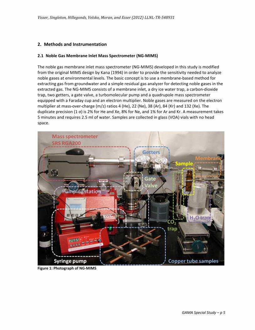
2. Methods and Instrumentation 2.1 Noble Gas Membrane Inlet Mass Spectrometer (NG‐MIMS) The noble gas membrane inlet mass spectrometer (NG‐MIMS) developed in this study is modified from the original MIMS design by Kana (1994) in order to provide the sensitivity needed to analyze noble gases at environmental levels. The basic concept is to use a membrane‐based method for extracting gas from groundwater and a simple residual gas analyzer for detecting noble gases in the extracted gas. The NG‐MIMS consists of a membrane inlet, a dry ice water trap, a carbon‐dioxide trap, two getters, a gate valve, a turbomolecular pump and a quadrupole mass spectrometer equipped with a Faraday cup and an electron multiplier. Noble gases are measured on the electron multiplier at mass‐over‐charge (m/z) ratios 4 (He), 22 (Ne), 38 (Ar), 84 (Kr) and 132 (Xe). The duplicate precision (1 σ) is 2% for He and Xe, 8% for Ne, and 1% for Ar and Kr. A measurement takes 5 minutes and requires 2.5 ml of water. Samples are collected in glass (VOA) vials with no head space.

Figure 1: Photograph of NG‐MIMS



Figure 2: Schematic of the NG‐MIMS system. A syringe pump draws the water (or gas) sample (blue) through the membrane inlet section (purple) where gases permeate the membrane into the mass spectrometer vacuum (red).

The NG‐MIMS consists of 4 sections: sample introduction, vacuum system, gas purification and mass spectrometry (Figure 1). In summary, a syringe pump is used to withdraw the water sample into a silicon tubing membrane. Water vapor is trapped in a U‐shaped water trap at ‐80C, CO2 is adsorbed in a trap and two getters are used to remove the abundant gases. The remaining noble gases are measured on an electron multiplier quadrupole mass spectrometer. A schematic of the system is presented in .

2.2 Vacuum system A total pressure of less than 5×10‐6 Torr is required to operate the electron multiplier of the mass spectrometer. The vacuum is provided by a pumping station (HiCube Eco, Pfeiffer Vacuum, Asslar, Germany) consisting of a turbomolecular pump and diaphragm backing pump. A gate valve is installed between the vacuum chamber and the turbo pump. The gate valve is used to throttle the pumping rate in order to optimize sample pressure in the mass spectrometer, while providing a faster pump down when opened fully. An additional rotary vane pump (Edwards .7 model) is used to evacuate the water trap and membrane section in order to reduce the load on the getters (not shown in ). Isolation valves between the sections are used to separate the getters and mass spectrometer from the water trap and membrane when the system is idle or when the water trap is pumped out. During measurements, all valves between the membrane and turbo pump are open, creating a continuous transfer of gas through the system from the membrane to the mass spectrometer. Because no valves have to be opened or closed for sample transfer during measurements, all valves are manual. 2.3 Sample introduction and membrane The membrane inlet consists of a 1‐1/3” CF liquid/gas feed‐through flange with two tubes (1/16” OD). A 20 cm length of silicone tubing (1/16” ID) connects the two tube ends inside the vacuum and acts as the gas transfer membrane. Water samples are drawn through the silicone tubing by a syringe pump (NE‐1000, New Era Pump Systems, Farmingdale, NY) at a constant rate of 0.5 mL/min (±1%). Compared to MIMS systems used for abundant gases, the low flow rate and long membrane on the NG‐MIMS provide a longer diffusion time for gas transfer into the vacuum. The sample is



withdrawn through the membrane into the syringe such that the sample does not come in contact with the pump until after passing through the membrane. Samples are typically collected in 12 mL or 40 mL clear or amber glass VOA vials with no headspace. Gas exchange with the atmosphere is minimized by drawing up the sample from the bottom of the uncapped vial. 2.3.1 Helium bag experiment To test the gas‐tightness of the VOA vial septa, two air equilibrated water (AEW) samples were stored in a zip‐lock bag filled with helium for 20 hours. One duplicate sample was capped with a standard septum cap, the other with an aluminum foil lining inside the cap. The partial pressure of helium in the bag (1 atm) was 250,000 times the natural partial pressure of helium in the atmosphere. Samples were removed from the bag several hours before measuring, to allow helium to escape from the cavities around the cap. The VOA with lining had a He/Ar ratio 25 times atmospheric. A wrinkle in the Al lining was noticed. The unlined VOA was measured on the Faraday Cup and a He/Ar ratio of over 2000 times atmospheric was measured.

Table 1: Results of helium diffusion through VOA septum caps.

He/Ar Ar/He (He/Ar)S/(He/Ar)atm

Air Equilibrated Water 0.015% 6584 1

Sample stored in VOA with foil 0.376% 266 25

Sample stored in VOA without foil 31.327% 3 2063

The helium concentration in the unlined VOA corresponds to a 1% re‐equilibration between the sample and sample container (bag), while the concentration in the Al‐foil lined VOA corresponds to a 0.01% re‐equilibration. Aluminum foil inside the VOA cap reduces diffusion through the cap by a factor of 100 and is necessary for reliable helium measurements if samples are stored more than 24 hours. Significantly less re‐equilibration is expected for the heavier noble gases, which have lower diffusivities and larger molecular sizes. 2.4 Gas purification While the membrane keeps liquid water out of the vacuum, water vapor diffusing through the membrane is trapped in a 40 cm U‐shaped stainless steel tube (¼”OD) immersed in a dry‐ice isopropanol slush at approximately 196 °K. Liquid nitrogen (77 °K) is not suitable because krypton and xenon sorb to stainless steel surfaces at temperatures below 150°K (Lott III, 2001). Approximately 3 grams of granular CarboSieve CO2 absorbent (Sigma‐Aldrich, St. Louis, MO) is used to remove CO2 from the dry gas mixture. A Zr‐alloy getter, consisting of 40 getter pills (WHC/4‐2, SAES getters, Italy) and one getter cartridge (C 50‐St707 on a SORB‐AC GP 50 getter flange, SAES getters, Italy), is used to capture abundant reactive gases (N2, O2, CO, CO2 and H2). During normal operation, the pills are heated to 400 °C using heater tape and the cartridge is heated to 225 °C by supplying 10V (1.25A) to the built‐in heater of the getter flange. Getter efficiency is assessed by examining measurements of nitrogen (N2) and argon (Ar) on the Faraday Cup (FC). The N2/Ar ratio of air is 84; it is 39 in AEW at 22 °C because of the higher solubility



of Ar. Due to differences in membrane separation and ionization efficiencies between the two gases, the observed N2/Ar ratio in a traditional MIMS system (similar to the Kana (1994) design) is 23: the Ar signal is only 4.4% of the N2 signal. In the NG‐MIMS system, the combined effect of the getter pills and cartridge is a nearly complete removal of O2 (<1% of Ar pressure) and a significant reduction of N2 to ~65% of Ar pressure. This represents a getter efficiency of 97% for N2. However, because of desorbing H2, the relative Ar pressure is only 37% of total pressure (“NG‐MIMS (gate open)” in Figure 3).

Figure 3: Relative abundances of argon and the reactive gases in air, air equilibrated water, and purified gas extracted from air equilibrated water.

Getter efficiency is further enhanced by adjusting the gate valve on the turbomolecular pump. The N2 signal is thereby reduced to 15% of the Ar pressure and the getter efficiency exceeds 99% for N2 (“NG‐MIMS (gate closed)”, Figure 3). With a sample flow rate of 0.5 mL/min through the membrane, the total pressure in the MIMS vacuum reaches 3x10‐6 Torr, more than 50% of which is Ar (1.8x10‐6 Torr). This total pressure is near the upper limit of the electron multiplier specifications and these are the optimal conditions for measuring noble gas isotopes. Theoretically, the getter efficiency can be increased by further throttling the gate valve and reducing the sample flow rate, but this is impractical for sample throughput. Also, at lower flow rates dispersion/diffusion in the sample line becomes an issue. 2.5 Mass spectrometer Noble gas isotopes are measured on the continuous dynode electron multiplier (CDEM) of a residual gas analyzer (RGA) quadrupole mass spectrometer (RGA‐200, SRS, Sunnyvale, CA). The RGA is controlled using the manufacturer‐supplied software. Measurements are made in Pressure vs. Time mode, hopping over the mass‐to‐charge ratios of five noble gas isotopes (4He; 22Ne; 38Ar; 84Kr; 132Xe) every 10 seconds to provide a high temporal resolution. Neon is measured on m/z 22 because doubly charged argon obscures the 20Ne signal. Argon is measured on m/z 38 because the 40Ar pressure exceeds the CDEM capabilities.



2.6 Procedures, calibration and data reduction Analysis by NG‐MIMS requires 5 minutes per sample. During the first three minutes, a constant gas transfer rate through the membrane is established. Measurements during the last 2 minutes (n=12) are averaged to reduce measurement noise. Unknown samples are referenced against AEW standards. Each set of 4‐6 samples is bracketed by standards (Figure 4). After every 3 or 4 sets of samples, flow through the membrane is stopped for at least 30 minutes and the background (“zero”) is measured by averaging 12 measurements at the end of the zero period. Both the standard and zero measurements vary by a few percent over the course of a day. Samples are therefore referenced against the two standard and zero measurements on either side by linear temporal interpolation.

Figure 4: Screen shot of a typical NG‐MIMS measurement run. In this case, a two and a half hour warm up period was used to reduce the background. The gate valve was closed at 2:25. Samples were measured in eight sets of six samples, bracketed by AEW standards on each side. The background was measured again after sets four and eight. Sample change is noticeable as small spikes caused by the stopping and starting of the syringe pump.

The noble gas isotope concentration is calculated as: Cs = Cstd * (Ms – Mi,zero) / (Mi,std ‐ Mi,zero) where Cs is the sample concentration, Cstd is the standard concentration, Mi,std and Mi,zero refer to the interpolated standard and zero pressure measurements. Noble gas isotope concentrations are then converted to total noble gas concentrations for each individual gas using known atmospheric isotope ratios.



2.6.1 Neon and CO2 interference Without cryogenic separation of the noble gases, each individual noble gas needs to be measured in the presence of all other noble gases along with the remainder of abundant reactive gases that are not captured by the traps and getters. This complicates the measurement of neon isotopes (20, 21, 22) due to the isobaric interference of doubly charged argon (40) on m/z=20, and of doubly charged CO2 (44) on m/z=22; and tailing of doubly charged argon (40) on m/z=21. Given these interferences, neon‐22 is most promising of the three neon isotopes for analysis by NG‐MIMS. Doubly charged CO2 causes an interference on the neon measurement at m/z=22. For air‐equilibrated water, CO2 constitutes 60‐75% of the m/z 22 signal. For samples with high dissolved CO2 concentrations, the CO2 signal at m/z 22 increases to nearly 100% and neon concentrations measured on these samples are highly uncertain, despite the CO2 trap in the NG‐MIMS. The source of CO2 in the NG‐MIMS appears to be both from naturally‐occurring dissolved CO2 in the sample and CO2 produced internally by reactions between water and the getter material or filament. While the CO2 trap is aimed at reducing CO2 from the sample, an additional correction is necessary in order to make a more accurate determination of the Ne concentration. To estimate the CO2 interference, 13CO2 is measured on m/z=45. (CO2 on m/z=44 exceeds the limits of the electron multiplier). This assumes that the variations in the δ13C of the measured CO2 are smaller than the uncertainty of the measurements (typically 2%) and therefore negligible. The contribution of CO2 to the m/z=22 signal is derived by linear regression between m/z=22 and m/z=45 for samples with known neon concentrations. The linear regression coefficient between m/z=22 and m/z=45 caused by CO2 interference is 0.595 ± 0.0032. This slope is used as the CO2 correction coefficient for neon measurements. The concentration of neon‐22 is then calculated as Cs = Cstd * [ (M

22s ‐ M

22i,zero) ‐ (M

45s ‐ M

45i,zero)*0.595] /[ (M

22i,std ‐ M

22i,zero) ‐ (M

45i,std ‐ M

45i,zero)*0.595]

where superscripts 22 and 45 refer to the respective m/z ratios. The uncertainty in the CO2 correction propagates into the uncertainty of the neon measurement. Uncertainty in the neon measurement is related to the CO2 correction as its fraction of the m/z=22 signal. Neglecting the uncertainty in the standard and background measurements (Mi,zero), the uncertainty of the neon measurement can be written as: UNe = (U22

2 + 0.5952*U452)0.5

Assuming the uncertainty to be proportional to the measured value, the relative uncertainty of the neon measurement is: UNe/Ne = U*(M22

2 + 0.5952*M452)0.5/(M22 ‐ 0.595*M45)

The uncertainty of the neon measurement increases by 50% if the CO2 correction represents 30% of the m/z=22 signal (typical for standards) and increases fivefold if the CO2 correction represents 75% of the signal (typical for groundwater samples).



3. Results of NG‐MIMS tests 3.1 Calibration experiments To test the linearity of the NG‐MIMS response, a range of binary mixtures of air equilibrated water (AEW) and boiled (degassed) water were measured. The mixture was made by withdrawing boiled water into the membrane using one syringe pump, and injecting AEW into the stream just before the membrane using a second syringe pump. The boiling water was cooled by drawing it directly through coiled stainless steel tubing immersed in a constant temperature water bath into the membrane. Maintaining the water flow through the membrane at a constant 0.5 mL/min using the withdrawal syringe pump, the mixture of AEW and degassed (boiled) water is controlled by the flow rate of the second syringe pump injecting AEW into the sample stream. The proportion of AEW was varied between 0% and 100% in 10% increments. In addition, proportions of 0%‐5% and 95%‐100% were tested in 1% increments. Measured partial pressures were found to increase linearly with increasing noble gas concentrations (Figure 5).

Figure 5: Measured partial pressures of noble gas isotopes (in Torr) increase linearly with increasing noble gas concentrations. Concentrations were varied from 0% to 100% of AEW, by online dilution with water that was degassed by continuous boiling.

From this experiment, the background and sensitivity of the instrument were calculated (Table 2). The higher background for helium is the result of the lower efficiency of the turbomolecular pump for helium. The background for argon, krypton and xenon is typically 1‐2% of the AEW measurements. The sensitivity is the combined effect of membrane diffusion, ionization and



detection efficiency and ranges nearly an order of magnitude between helium and xenon. Note that the sensitivity of the instrument is calibrated against two AEW standards for each unknown measurement. The precision was calculated as one standard deviation of the residuals of the regression divided by the AEW pressure. The detection limit as percentage of CAEW was calculated as the background plus three times the precision.

Table 2: Results of the mixing calibration experiment.

Analyte CAEW

[ccSTP/g] PBackground [Torr]

PAEW [Torr] Back

ground

Sensitivity [Torr/

(ccSTP/g)]

Residuals [Torr]

Precision Detection

limit [ccSTP/g]

He‐4 4.44E‐08 1.27E‐12 1.63E‐11 7.8% 3.68E‐04 1.80E‐13 1.1% 11%

Ne‐22 1.67E‐08 9.96E‐12 3.97E‐12 ‐ 2.37E‐04 1.16E‐13 2.9% ‐

Ar‐38 1.86E‐07 5.69E‐12 2.60E‐10 2.2% 1.40E‐03 3.38E‐12 1.3% 6%

Kr‐84 3.69E‐08 5.74E‐13 4.76E‐11 1.2% 1.29E‐03 9.91E‐13 2.1% 8%

Xe‐132 2.34E‐09 5.13E‐14 2.87E‐12 1.8% 1.23E‐03 7.15E‐14 2.5% 9%

3.2 Duplicate precision and accuracy For various research projects, a total of 62 samples were measured in duplicate. The precision of the NG‐MIMS (Table 3) is calculated from the differences between duplicates of these unknowns as:

∑

where x1 and x2 are the duplicate measurements and n is the total number of samples. The relatively lower precision of helium measurements (2.1%) reflects the volatility of helium and the relatively high background due to the limited pumping efficiency of the turbomolecular pump. The low precision of neon measurements (7.8%) is the result of the correction for CO2 interference. Argon and krypton are more abundant and can be measured with greater (1.0%) precision than xenon (1.5%). 3.3 Comparison with a traditional noble gas mass spectrometer To compare the accuracy of the NG‐MIMS with a traditional NGMS, 35 samples collected in clamped copper tubes were measured on both the NG‐MIMS and the traditional noble gas mass spectrometer (NGMS) at LLNL. In the NGMS, the entire water sample is introduced into the vacuum and degassed. Water is frozen out into a stainless steel container at dry ice temperature. The abundant gases are removed by getters. Noble gases are cryogenically separated on a cold finger. Noble gas abundances are measured on a static sector field mass spectrometer (He, Ne and helium isotope ratio), by pressure measurement (Ar) and by an RGA quadrupole mass spectrometer (Kr, Xe) (Cey et al., 2008). The comparison between the NG‐MIMS with a traditional NGMS based on 35



copper tube samples is shown in figure 6. Only one copper tube was available for each measurement and the comparison is based on single data points (rather than duplicate averages).

Figure 6: Comparison of data for samples analyzed on the NG‐MIMS and on the traditional noble gas mass spectrometer system at LLNL. Horizontal and vertical lines indicate NGMS uncertainty and NG‐MIMS duplicate precision respectively. Circles indicate samples with bad fit (Cey et al., 2008) of Ar, Kr and Xe measurements to solubility and excess air models. Although individual gases may be successfully modeled for bad fit samples, all gas data from these samples are excluded from statistical comparison.

Groundwater samples typically have noble gas concentrations in excess of atmospheric equilibrium, and goodness of fit to an “excess” air model (Aeschbach‐Hertig et al., 2000) is often used to assess data quality . Goodness of fit measures the ability of an “excess air” model to describe the observed data, and is judged on the probability that the sum of the weighted squared deviations between the modeled and measured concentrations for Ar, Kr, and Xe could arise by chance (based on a chi‐square distribution). If that probability is less than 5%, the sample is judged to have bad fit (Cey et al., 2008). For this comparison, only NG‐MIMS samples for which Ar, Kr, and Xe data fit an equilibrium or unfractionated excess air model were used for comparison to traditional NGMS data. Helium was excluded from the calculation of goodness of fit because of the possibility that radiogenic helium was present in these samples. Neon was excluded because of its higher uncertainty. Of the 35 NG‐MIMS samples run, 33 samples fit to both models and two did not give a probable (≥1%) fit. No fit indicates a measurement error or sampling problem, and these samples were excluded from the comparison with the NGMS.



Based on the remaining 33 samples, the uncertainty of the NG‐MIMS measurements based on the reproducibility of the NGMS measurements was calculated as:

∑ 1

where U is the measurement uncertainty (%), Y is the NG‐MIMS result for noble gas i, X is the NGMS result for noble gas i, and n is the number of samples included in the comparison (33). The uncertainty of NG‐MIMS measurements would likely be ~30% lower if the statistic is based on duplicate measurements. It should also be noted that this statistic includes the uncertainty of the NGMS. The relative bias (B) of the NG‐MIMS measurements against the NGMS measurements was calculated as

∑ 1

The duplicate precision, uncertainty and bias of the NG‐MIMS are listed in Table 3. The measurement uncertainty for helium is 16% and the bias is ‐8.7%. Both the uncertainty and bias are likely due to its volatility and resulting escape from the sample to the atmosphere, as the container is open during NG‐MIMS measurements. Helium measurements are sufficiently accurate for the detection of a terrigenic helium component, but not for quantification of radiogenic helium age. The neon uncertainty and bias are 40% and ‐14%, due to both its volatility and the necessary CO2 interference correction. At this stage, neon measurements are not yet suitable for excess air calculations. Lacking helium and neon measurements, excess air calculations need to be performed using argon, krypton and xenon concentrations. The uncertainty of these measurements is 6.4%, 4.4% and 6.0% respectively. The apparent bias of these measurements is 3.2%, 2.4% and 4.6%, respectively. While this is not sufficient for accurate paleoclimate reconstructions (5% uncertainty for xenon represents a temperature uncertainty of ~2 °C), these measurements are suitable for detecting variations in recharge/equilibration temperature (see below) and can easily distinguish between natural variation in noble gas concentrations and relevant introduced noble gas tracer concentrations.

Table 3: Duplicate precision, measurement uncertainty and bias of the NG‐MIMS system. Values in parentheses show measurement uncertainty

of traditional LLNL noble gas mass spectrometer.

Duplicate precision (%)

Measurement uncertainty (%)

Measurement bias (%)

Helium 2.1 16 (2) ‐8.7

Neon 7.8 40 (2) ‐14

Argon 1.0 6.4 (3) 3.2

Krypton 1.0 4.4 (3) 2.4

Xenon 1.5 6.0 (3) 4.6



3.4 Noble gas temperature estimates To test the capability of the NG‐MIMS to reconstruct equilibration temperatures, a number of AEW samples were measured. Deionized water was set out to equilibrate with the ambient laboratory air, in a laboratory refrigerator (4 °C) and in a temperature controlled water bath (22.5 ‐ 30 °C). Additional surface water samples were collected from a mountain stream (~0 °C) and from the surface of an artificial recharge pond with an average depth of 10 m and a measured surface temperature ranging from 10 °C to 21 °C. Samples were collected in 12 or 40 mL glass vials with no head space. The equilibration temperature was estimated by minimizing the error‐weighted residuals of argon, krypton and xenon (Figure 7). Samples collected from the mountain stream show noble gas concentrations in equilibrium with the field‐measured water temperature. Noble gas temperatures of water equilibrated in a refrigerator overestimate the measured water temperature, possibly due to incomplete equilibration (see below). Samples from the pond show scatter around the measured surface water temperature, due to incomplete equilibration and daily surface water temperature fluctuations. Laboratory AEW samples show scatter, but no bias. Noble gas concentrations in samples collected from the temperature controlled water bath appear to underestimate the measured water temperature. Excluding the pond water samples, the mean error (ME) and root mean square error (RMSE) of the noble gas temperature estimates are ‐0.27 °C and 1.17 °C.

Figure 7: Estimated noble gas equilibration temperatures of air equilibrated water (AEW) samples (a), noble gas temperature errors (b), apparent equilibration temperatures during the equilibration of noble gas concentrations with ambient temperature in fridge and water bath (c), and measured temperatures of recharge pond and noble gas estimated equilibration temperatures (d).



To monitor the equilibration process, samples were collected from the refrigerator and water bath after 0, 1, 2, 3, 4, 8, 10, 15 and 17 days (Figure 7c). The estimated noble gas temperatures show that the concentrations in the water bath change relatively quickly and are in equilibrium with the new temperature after 4 days. The concentrations in the refrigerator change more slowly. While the concentrations appeared to have stabilized after 8 days, the estimated noble gas equilibration temperature was still 2 °C above the measured water temperature. Between October 10, 2011 and February 9, 2012, 14 samples were collected from the surface of the recharge pond, while the water temperature changed during that period from 21 °C to 11 °C (Figure 7d). The estimated noble gas equilibration temperatures appear to lag behind, and all (except one outlier) overestimate the pond surface water temperature, until the temperature stabilized and the noble gases had sufficient time to equilibrate. 3.5 Heating experiment To demonstrate the real‐time capability, the NG‐MIMS was used to measure the noble gases dissolved in water while heating the water to 70 °C. A 500 mL beaker was filled with 250 mL DI water at room temperature. The water was stirred and heated to 70 °C on a hotplate. The water was sampled by the NG‐MIMS at a rate of 0.5 mL/min and the noble gases were measured every 10 seconds. Two‐minute averages (n=12) are plotted in Figure 8.

Figure 8: Evolution of noble gas concentrations (measured by the NG‐MIMS) while heating a stirred, open beaker of water. Concentrations are reported as fraction of the starting air equilibrated values. Equilibrium concentrations determined by the temperature dependent noble gas solubility coefficients (Ozima and Podosek, 2002) are shown with dashed lines.



As a result of the heating, the noble gases escaped to the atmosphere driven by the lower solubilities at higher temperatures. Noble gas concentrations respond rapidly to changing water temperatures under these experimental conditions. While the temperature of the water was rising, the noble gases were in disequilibrium with the atmosphere. Approximately ten minutes after the temperatures reached its final value, the noble gas concentrations reached a new equilibrium. However, the new equilibrium concentrations were lower than predicted by the usual temperature dependent solubility models (Clever, 1979; Ozima and Podosek, 2002; Weiss, 1971; Weiss and Kyser, 1978). The cause of this discrepancy is yet unknown. 3.6 Bubbling experiment The ebullition of biologically generated gases has been shown to decreases noble gas concentrations in a variety of settings such as groundwater, lake sediments and peat cores (Amos et al., 2005; Baedecker et al., 1993; Blicher‐Mathiesen et al., 1998; Brennwald et al., 2005; Laing et al., 2008; Solomon et al., 1992; Sültenfuβ et al., 2011; Visser et al., 2007). A better understanding of the processes controlling noble gas loss may allow for improved noble gas constraints on biogenic gas fluxes. The NG‐MIMS is especially well suited to address this dynamic process with real‐time measurements. To demonstrate this capability, the NG‐MIMS was used to measure the noble gases dissolved in water while bubbling N2 gas through the water column. A 24 cm tall 100 mL graduated cylinder was filled with DI water and the top was covered with plastic foil with holes to allow for advective escape of the N2 gas. The water was sampled from one cm above the bottom of the graduated cylinder. After five minutes, N2 gas was bubbled through the water column from the bottom of the cylinder at a rate of 24 mL/min.

Figure 9: Results of real‐time NG‐MIMS measurements of noble gas concentrations in a column of water while sparging with N2 gas.



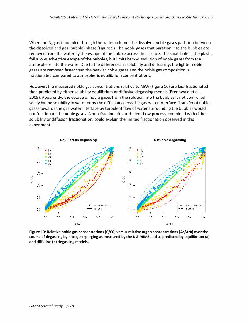
When the N2 gas is bubbled through the water column, the dissolved noble gases partition between the dissolved and gas (bubble) phase (Figure 9). The noble gases that partition into the bubbles are removed from the water by the escape of the bubble across the surface. The small hole in the plastic foil allows advective escape of the bubbles, but limits back‐dissolution of noble gases from the atmosphere into the water. Due to the differences in solubility and diffusivity, the lighter noble gases are removed faster than the heavier noble gases and the noble gas composition is fractionated compared to atmospheric equilibrium concentrations. However, the measured noble gas concentrations relative to AEW (Figure 10) are less fractionated than predicted by either solubility equilibrium or diffusive degassing models (Brennwald et al., 2005). Apparently, the escape of noble gases from the solution into the bubbles is not controlled solely by the solubility in water or by the diffusion across the gas‐water interface. Transfer of noble gases towards the gas‐water interface by turbulent flow of water surrounding the bubbles would not fractionate the noble gases. A non‐fractionating turbulent flow process, combined with either solubility or diffusion fractionation, could explain the limited fractionation observed in this experiment.

Figure 10: Relative noble gas concentrations (C/C0) versus relative argon concentrations (Ar/Ar0) over the course of degassing by nitrogen sparging as measured by the NG‐MIMS and as predicted by equilibrium (a) and diffusive (b) degassing models.



3.7 Gas sample To investigate the cause of high dissolved gas pressures observed in a ‘pump and treat’ remediation well at the LLNL‐site, a gas sample was collected in a Tedlar bag from the gas‐separation device on the remediation well. The pressure of the gas in the system was not known. The relative concentrations of the noble gases were measured on the NG‐MIMS, referenced against atmospheric air. The sample was drawn through the membrane similar to a water sample. The gate valve was opened to reduce the sensitivity, in order to compensate for the higher rate of gas diffusion through the membrane. Additionally, the abundant gases (N2, O2, Ar) were measured on a traditional MIMS system. The fractional concentrations of the gases (relative to atmospheric) in the sample are shown in Figure 11. For example, nitrogen makes up 97% of the gas sample, versus 78% of the atmosphere. The fractional concentration relative to the atmosphere is therefore 97%/78%=125%. The measured relative concentrations of noble and abundant gases correspond to a headspace in equilibrium with a groundwater with the following characteristics: a recharge temperature of 20 °C at an altitude of 200 m, 0.0018 ccSTP/g of excess air, 0.0088 ccSTP/g of excess N2 (from denitrification of 49 mg/L NO3) and consumption of 87% of the initially dissolved oxygen. The total dissolved gas pressure corresponding to this mixture is 1.48 atmospheres. In this particular setting, the gas‐phase in the gas‐separation device acted as a passive diffusion sampler (Gardner and Solomon, 2009).

Figure 11: Fractional concentrations of noble gases measured in gas sample, relative to atmospheric.



4. Field Test: Rapid Xe tracer results with the NG‐MIMS 4.1 Noble gas tracer selection An inert noble gas tracer was introduced into a recharging water source, and its arrival at down‐gradient receptors (monitoring wells and production wells) was monitored. In choosing a noble gas tracer, both the cost of the tracer gas and the gas’s properties were considered. Because long‐screened production wells are key sampling points, about 1% of the tagged water should ideally be detectable when mixed in with ambient groundwater. Therefore, a 100‐fold dilution of the introduced tracer needs to cause a significant deviation from the natural variation in the background concentration, and also a significant deviation from the measurement uncertainty. For example, assuming a 5% measurement uncertainty, the initial tracer concentration needs to be 10 times the natural background concentration to produce a 10% (2 σ) change in concentrations at a 100‐fold dilution. The natural variability of noble gas concentrations is the result of variations in recharge temperature (affecting mostly Kr and Xe), variations in the amount of excess air (affecting mostly He and Ne), and addition of terrigenic helium. Figure 12 shows the effect of recharge temperature and the incorporation of excess air on dissolved noble gas concentrations.

Figure 12: Concentrations of noble gases (relative to solubility equilibrium concentration at 0°C) as a function of temperature (a) and after addition of 10 ccSTP/L of excess air (b).

Table 4 shows the effects of variations in recharge conditions on noble gas compositions. Under typical meteorological conditions in the SF Bay area, the temperature of an artificial recharge pond can vary between 10°C and 20°C. At 20 °C, the equilibrium concentrations are lower by 4% (He) to 28% (Xe) than at 10 °C. However, the ratio of Xe/Kr changes by only 6%. Addition of a typical amount of excess air (6 ccSTP/g) will increase the neon concentration by 50% while the xenon concentration will increase by only 4%. The Xe/Kr ratio decreases by 3% in response to 6 ccSTP/g excess air. These examples show that the xenon concentration is least variable, and the variation is largely the result of variation in recharge temperature and predictable from the concentrations of the other noble gases.



Table 4: The effects of variations in recharge conditions on dissolved noble gas compositions.

C=concentration, T=temperature, EA=excess air

Scenario He Ne Ar Kr Xe Xe/Kr

C(T=20)/C(T=10) 96% 92% 81% 77% 72% 94%

C(T=10,EA=6ccSTP/g)/C(T=10) 163% 150% 113% 107% 104% 97%

The properties and the natural occurrence of the noble gases can be used to determine the amount (and hence the cost ) of tracer that would be required to tag recharge water. In Table 5, these calculations are done for one million cubic meters of water, and show that xenon appears to be most feasible introduced noble gas tracer in terms of required tracer volume and cost. Xenon is the most soluble of the noble gases, making it well suited to be a water tracer. The high solubility does not result in high natural background because xenon also has the lower atmospheric concentration of the noble gases, and in fact has the lowest dissolved natural water concentration and the lowest natural inventory in one million cubic meters of water. These attributes in conjunction with the low measurement uncertainty of the NG‐MIMS for xenon (6%) mean that only a small amount of tracer (~80 L) need be added to raise the source water concentration sufficiently to be able to see a 100:1 dilution at a receptor site. The amount of tracer required is determined by the background concentration in the source water, the variability in that concentration, and the uncertainty in the measurement. The natural variation in neon and argon concentrations, which are relatively insoluble, is large due to the presence of variable amounts of excess air. The presence of terrigenic helium contributes significantly to the uncertainty in background helium concentrations and cannot be assessed based on other measured parameter. This uncertainty in background concentration and the potential to interfere with 3H/3He groundwater dating of recharged waters exclude helium as a viable tracer. The measurement uncertainty of the NG‐MIMS is lowest for argon, krypton and xenon (4‐6%). The concentration change at the well that is required in order to detect the tracer is determined by natural variability and measurement uncertainty, both of which are lowest for krypton and xenon. Therefore, the required concentration change in the source water is also lowest for krypton and xenon. Because of the low natural concentration of xenon, only 81 liters is required to sufficiently tag 1 million cubic meters of water. Because xenon is the most soluble noble gas with the lowest diffusion coefficient, its escape to the atmosphere is limited. Despite its relatively high cost ($8/L) compared to helium or argon ($0.01/L), xenon is the most feasible noble gas tracer. Therefore, xenon was selected as the noble gas tracer for the field‐scale experiment. In an experiment in which two tracers are desired (for two recharge sources or covering two time periods), krypton and xenon are feasible choices, and could be sampled and analyzed simultaneously.



Table 5: Properties of noble gases, required amount, cost and feasibility of the noble gases as introduced tracers

Noble gas Helium Neon Argon Krypton Xenon SF6

Atmospheric abundance (ppm)

5.1 18 9200 1.1 0.086 0.00001

Solubility @ 1 atm (L gas/m3 water)

9 12 43 83 158 9

Inventory (L) in 106 m3 water

47 206 392,255 93 13 0.00009

Source of variability in groundwater

Radiogenic helium

Excess air Excess air; Recharge temp.

Recharge temp.

Recharge temp.

Excess air; GW age

Natural variability in groundwater

100% 50% 10% 6% 6% 100%

NGMIMS/GC* Measurement uncertainty

16% 40% 6% 4% 6% 5% *

Required concentration change at well to detect tracer

101% 64% 12% 7% 8% 100%

Required increase in source water concentration to see 100:1 dilution at receptor well

100x 50x 10x 6x 6x 100x

Tracer required (L / 106 m3)

4,707 10,298 3,922,545 557 81 17(1)

Tracer required (L / acre‐ft)

5.8 12.7 4,837 0.7 0.1 0.02

Tracer cost ($/L)

$0.01 $0.30 $0.01 $2.00 $8.00 $1.00

Tracer cost ($/106 m3 water)

$47 $3,089 $39,225 $1,114 $648 $17

Tracer cost ($/acre‐ft water)

$0.06 $3.81 $48.37 $1.37 $0.80 $0.02

Feasibility Large volume

Too large volume, expensive

Too large volume, too

expensive

Small volume, low cost

Smallest volume,

lowest cost

Green‐house gas



4.2 Tracer introduction method Gas tracers can be introduced in artificial recharge ponds in three ways:

1. dissolution of the tracer gas into a limited quantity of water in the laboratory and release of the saturated solution into the pond

2. bubbling the gas through the water column 3. diffusion of the gas through gas permeable tubing (diffusion tubing) submerged in the pond.

Pre‐dissolution is limited to small quantities of tracer gas to be dissolved (suitable for enriched isotope tracers). Previous studies of bubbling SF6 through the water column show that the dissolution efficiency may be as low as 4% (McDermott et al., 2008), which is not economical for xenon. Introduction by diffusion tubing (Cook et al., 2006; Sanford et al., 1996) has the great advantage that little or no tracer gas is directly lost to the atmosphere. This injection method also leads to less uncertainty in the rate of introduction. In this experiment, xenon was introduced by gas diffusion through silicone tubing suspended in the water column of an artificial recharge pond. 4.3 Laboratory‐scale xenon tracer introduction experiment Before application at the field scale, a small laboratory introduction experiment was conducted to assess the xenon dissolution rate. Xenon was introduced into a miniature version of the recharge pond (a cooler) through a short piece of silicone tubing. The experiment was not to scale. The dimensions of the cooler were 56x28x25 cm and the length of the tubing was 17.5 cm. The relative scaling from lab (cooler) to field (pond) experiments was several orders of magnitude larger for the tubing length than for the water volume. As a result, the concentrations of xenon were several orders of magnitude higher than expected in the real pond. The cylinder containing 999 L of xenon was attached to a 17.5 cm length of 1 mm diameter silicone tubing via a pressure regulator set at 0.7 bar gauge pressure. The tubing was placed at the bottom of the cooler filled with tap water on 2011/09/12 at 10:30 AM. The silicone tubing was removed after 95.5 hours (2011/09/12 at 10:00 AM). 4.3.1 Samples and measurements Samples were collected by submersing VOA vials and capping them under water, while making sure that no bubbles were entrapped. (No aluminum foil was used to line the VOA cap.) Samples were collected every 30 minutes for 4 hours, every hour for 4 more hours, and twice daily afterwards. A similar sampling scheme was followed after removing the tubing to study the diffusive escape of xenon from the cooler. Because of the expected high concentrations, samples were measured on mass/charge 132 on the Faraday Cup of the NG‐MIMS. To increase the measurement range of the NG‐MIMS, most of the samples were measured twice: at low sensitivity with the gate valve open and at higher sensitivity with the gate valve 21/8 turn closed (the normal procedure for measuring natural samples on the electron multiplier).



4.3.2 Calibration To calibrate the NG‐MIMS, a saturated xenon solution (xenon partial dissolved gas pressure of 1 atm) was created in a 10 mL syringe. The syringe was filled with 4 mL of water and 6 mL of xenon gas from a gas sampling bag. The water and gas were equilibrated by shaking for 1 minute. The 6 mL gas was purged and 6 mL of pure xenon gas was drawn into the syringe again. The procedure was repeated 5 times yielding (in theory) a xenon solution in equilibrium with xenon at 1 atm (>99% pure) and <1% of other gases. The calibration solution was mixed online with AEW to create 0.5%, 1%, 2%, 5% and 10% Xe solutions using two syringe pumps (Figure 13). The mixed solutions were measured on the Faraday Cup with the gate valve open. The slope of the measured pressures vs the calculated concentrations (sensitivity of the NG‐MIMS Faraday Cup to xenon) was in good agreement with the calculated sensitivity to argon in AEW (3.87×10‐4 Torr per ccSTP/g for xenon vs 3.20×10‐4 Torr per ccSTP/g for argon).

Figure 13: Calibration of the NG‐MIMS using dilutions of water saturated with xenon at room temperature.



4.3.3 Results of laboratory‐scale tracer test Bubbles appeared on the outside of the tubing 30 minutes after the tubing was put in the cooler. The gas pressure inside the tubing was greater than 1 atm so the total dissolved gas (xenon) pressure just outside the tubing exceeded the hydrostatic plus barometric pressure, allowing bubbles to form. Apparently, the transfer rate through the tubing wall exceeded the dissolution rate of xenon. The formation of bubbles around the tubing increases the effective surface area across which xenon can dissolve. Xenon concentrations in the cooler show a nearly linear increase over the entire introduction period of 95 hours (Figure 14). The dissolution rate in the first 4 hours is 26 ccSTP/m3/h, equivalent to 5.8 ccSTP/h per meter tubing. This is 5 times the release rate of 1.15 ccSTP/h/m published by Cook (2006) who introduced SF6 into a stream at a lower gauge pressure (0.6 bar vs 0.7 bar). The dissolution rate decreases slightly over time to about 20 ccSTP/m3/h. After the tubing was removed, xenon appears to escape to the atmosphere at an initial rate of 36 ccSTP/m3/h. The xenon concentration decreases exponentially as expected with diffusive escape where the rate is dependent on the concentration gradient. The fact that the escape rate during the first hours after the tubing was removed is higher than the initial dissolution rate is surprising. Perhaps the frequent sampling after removing the tubing (and mixing in the cooler) increased the release rate. Also the formation of bubbles may have increased the dissolution rate after a few hours.

Figure 14: Laboratory scale tracer test, labeling water in a cooler with xenon gas. Xenon was introduced through diffusion tubing for approximately 100 hours. The diffusion tubing was then removed, and the water was allowed to return toward background concentrations.

The silicone diffusion tubing was very effective at introducing xenon to the water in the cooler. The success of this laboratory‐scale test indicated that this approach should work well at the field scale. The rate at which the xenon concentration increases in the cooler depends on the dissolution rate of xenon across the surfaces of the bubbles that form on the outside of the tubing. The prevalence of



bubbles might be minimized at the pond scale, by placing the diffusion tubing deeper underwater than was possible in the cooler. 4.4 Field‐scale tracer site Alameda County Water District (ACWD) operates a number of artificial recharge ponds in the Fremont area that were considered suitable for a field‐scale experiment to test the xenon tracer approach. Kaiser Pond was selected (Figure 15) in part because a similar tracer experiment had been conducted by LLNL in 1997 at the same site. That experiment used isotopically‐enriched xenon tracers (Moran and Halliwell, 2003) and the collected data provided background information on expected mixing ratios and travel times. In this current study, the xenon tracer was not isotopically‐enriched. ACWD expected to divert water into Kaiser Pond in the fall of 2011, which would coincide with the tracer introduction. The increased water level in the pond would be beneficial to push the tagged water into the aquifer. ACWD committed staff to support introduction of the tracer, as well as during the continued sampling of surface water and groundwater. Boat access to the pond was available for the installation of the diffusion tubing and monitoring of the pond. ACWD’s Kaiser Pond has a volume of 1040 acre‐feet (1.28 x 106 m3) and a surface area of 25 acre (1.0 x 105 m2). It naturally contains about 12.6 liter xenon at standard temperature and pressure. Increasing the background concentration by ten‐fold would require 126 L STP xenon, at a cost of approximately $1,000.

Figure 15: Photo composite of the study site at Kaiser Pond, as seen from the bank above the boat ramp looking ENE.

Water from the artificial recharge pond discharges at a drinking water production well field located 350 m away from the pond. The production well field consists of 8 production wells, although not all wells are typically pumped at the same time. In addition to the production well field, four monitoring wells are available between the pond and the well field. Figure 16 shows the dimensions of the pond and the relative locations of the wells. ACWD does not use recycled water for its recharge ponds, and has no plans to do so. Therefore, the 6 month criterion for travel would not apply to ACWD under proposed state regulatory criteria. Earlier studies with Macroscopic Particle Analysis showed that water pumped at the well field is not “groundwater under the influence of surface water,” as defined by federal and California regulations.



Figure 16: Map of the tracer study site.

4.5 Tracer introduction Assembly of the diffusion tubing array was completed by one worker in one day. The array consisted of a 152 m (500ft) length of PVC tubing to feed the xenon to the silicone diffusion tubing. Every 15 m (50 ft), two 15 m (50 ft) lines of silicone tubing branched off and ran along the PVC feed line (Figure 17). The parallel PVC and diffusion lines were tied together to mason line that would be tied to anchors and buoys to keep the line in place. This setup provided a distributed introduction of xenon along a 150 m length, easy deployment in the field and limited risk of failure. The completed xenon diffusion system was installed in the pond on 17 October 2011 from a small boat. First, the diffusion tubing array was laid out at the surface by tying the mason line every 7.6 m to a buoy, held in place by a brick sunk to the bottom. Second, the entire diffusion system was connected to the xenon cylinder (via a pressure regulator set at 100kPa) on the shore of the pond. The cylinder contained 995L STP of xenon, compressed into 16 L at 900 PSI (62 bar). Third, the diffusion line system was submerged to 6 m below the surface by tying it to the vertical lines between the anchors and buoys. Just before the line was submerged, the ends of the diffusion tubing were cut and vented to remove the air from the tubing, then closed off by a knot. Installation of the diffusion tubing system took less than 4 hours, and was completed using two workers to lay out the line and a boat operator.



Figure 17: Schematic representation of tracer introduction line

The pressure of the xenon cylinder was checked on 10/20/2011, after three days of introduction. The observed pressure (750 PSI = 52 bar) was within expected range (indicating about 166 L of xenon was introduced) and the setup was not altered. The entire system was removed on 10/24/2011, after 7 days. At that time, the pressure in the cylinder had dropped to 190 PSI (= 13.8 bar), indicating that about 774 L of xenon had been introduced. The larger than expected drop in xenon pressure may have been caused by a leak in the diffusion tubing system. 4.6 Pond monitoring In order to monitor the introduction of xenon into the artificial recharge pond, the pond was repeatedly sampled at 14 different locations. Vertical profiles (3 m sample intervals) were collected at four locations. Samples were collected in 40mL VOA vials. The vials were filled from the surface of the pond, or pumped from greater depths using a peristaltic pump. Temperature, conductivity, pH and dissolved oxygen were measured using a YSI multi‐meter at each sampling. A total of 86 samples were collected from the pond and measured during the first 14 days of the experiment. Reported xenon concentrations are relative to the xenon concentration and Xe/Kr ratio of the NG‐MIMS water standard, equilibrated with the atmosphere at 18°C and 151m altitude. Reported xenon concentrations greater than one do not necessarily constitute a detection as there is slight variation in the background Xe concentration. After 7 days, xenon concentrations averaged around 60 times background, but varied horizontally between 44 (away from introduction line) and 170 (near introduction line) times background. After 10 days (3 days after removing the introduction line), xenon concentrations averaged around 55 times background and varied only between 49 and 59 times background. Based on these data (shown in Figure 18), we conclude that the pond was well mixed horizontally.



Figure 18: Xenon concentrations relative to AEW at the surface of the pond, after 7 days of introducing xenon (left) and three days after removal of the introduction line (10 days after the start of the introduction, right). Green line indicates the location of the introduction line. Light brown circles in pond show sample sites for surface water collections with adjacent xenon concentration; dark brown circles indicate monitor well locations (MW1 through MW8).

The vertical temperature profile recorded at the middle of the pond shows a thermocline at 9 m below the surface (Figure 19). The thermocline coincides with a drop in dissolved oxygen, indicating limited mixing between the top and bottom part of the pond over the sampling period. Vertical profiles of xenon confirmed this stratification of the water column. The top 6 m of the pond appeared to be vertically well‐mixed, as the concentrations were nearly constant with depth. The concentration at 15 m depth increased after 10 days from the start of the introduction. Xenon concentrations across the pond quickly converged after the introduction was stopped (Figure 20). The sample collected from the boat ramp was therefore determined to be representative of the average pond concentration. After two weeks following sample introduction, xenon concentrations in the pond were monitored by collecting a sample from the boat ramp instead of accessing the interior of the pond by boat. The xenon concentrations in the pond decreased nearly exponentially during the first three weeks, following the equation Ct = 114 e

(‐0.055 * t) with C relative to the standard concentration and t in days since the start of the introduction. The exponential decrease of the xenon concentration in the pond shows that with respect to diffusive escape to the atmosphere, xenon has an effective half‐life in the pond of 12.6 days.



Figure 19: Vertical profiles of temperature, dissolved oxygen and xenon collected near the middle of the pond.

Based on the mixing depth derived from the vertical profile and the decrease in xenon in the pond, the introduction of xenon can be modeled using a simple mass balance model: Ct+dt × V = Ct × V + Xeintr ‐ Xeesc where Ct is the concentration of xenon at time t, V is the mixed volume of the pond (10 m deep, 106 m (720 acre‐ft)), Xeintr is the amount of xenon introduced and Xeesc is the amount of xenon escaped to the atmosphere. The introduction rate is assumed to be constant between day 0 and day 3 and between day 3 and day 7, although it is uncertain at which time the potential leak started. The xenon escape rate was derived by fitting an exponential equation (Ct = 114 e

(‐0.055 * t)) to the decreasing xenon concentrations after the end of the introduction period. A gas exchange velocity of 0.55 m/d across the surface of the pond was derived from the coefficient in the exponential function, and the xenon escape rate can then be calculated as: Xeesc = Ct*A*‐0.55*dt where A is the surface area of the pond (105 m2). Assuming the introduction method is 100% efficient in dissolving xenon into the pond, the concentration of xenon after 7 days is underestimated by 11%, possibly due to incomplete mixing. After 10 days, the model predicts the xenon concentrations within 3% (Figure 21). This shows that the introduction method is practically 100% efficient and no xenon is lost to the atmosphere, other than diffusion across the pond surface. This compares to reported losses of up to 97% for similar tracer experiments in which the gas tracer was introduced using a submerged bubbler (Clark et al., 2005, McDermott, 2008).



Figure 20: Xenon concentrations in the pond, relative to AEW at 18 °C.

Figure 21: Measured and modeled concentrations of xenon in the pond mixed layer.



4.7 Xenon concentrations and arrival times in monitoring wells

Xenon concentrations in monitoring wells were sampled bi‐weekly for two weeks and once every two weeks afterwards (Figure 22). Xenon was detected in MW1 three days after the start of the introduction at 20% of the concentration of xenon in the pond on the same day. The effective travel time to this monitoring well, located close to the shoreline, is therefore less than three days. The xenon concentration in MW1 was approximately constant at 20% of the pond concentrations until 23 days after the start of the introduction. Since then, the concentration in MW1 decreased from 5 to 3.6 times background, while the pond concentration decreased from 25 to 3.6 times background. It appears as if the fraction of pond water in this monitoring well (which has a 12 m perforated interval) increased from 20% to nearly 100% over the same time period. The introduced tracer was not detected in any other monitoring well until 80 days after the start of the experiment. The sample from MW2 on day 80 contained a relative xenon concentration of 1.36 times background. While the increased concentration is not significant, the Xe/Kr ratio (relative to the standard) measured an increase of 25%, indicating a new positive tracer detection (Figure 23). Starting at day 101, tracer water was also detected at MW4, with 41% excess xenon and a 22% elevated Xe/Kr ratio. 4.8 Xenon concentrations and arrival times in production wells Over the course of the experiment to date, 61 production well samples have been collected and analyzed for xenon. For the first 115 days of the experiment, the measured xenon concentrations varied between 1.17 and 1.27 times the AEW standard ( Figure 24) and indicated recharge temperatures below 18°C. The Xe/Kr ratio over this period did not vary by more than 6%. Based on these ratios we conclude that tracer‐xenon was not detected in the production wells in the first 115 days (Figure 25). The first xenon detection in the production well field occurred in water sampled 136 days after the tracer application date. On this day the xenon concentrations increased to 1.56 times the AEW standard, and the Xe/Kr ratio increased by 33%. This production well xenon concentration is 0.7% of the peak xenon concentration observed in the recharge pond. The observed concentration is similar to that observed in the previous tracer study carried out in 1998 (Moran and Halliwell, 2003); however the observed first arrival travel time is about twice as long. The observed differences are likely the result of contrasting weather patterns, pond loading, and well field pumping between the first experiment, carried out during a very wet year, and the present experiment, carried out during a year of below average precipitation.



Figure 22: Xenon concentrations measured in monitoring well samples. Connecting lines are for visibility only and do not imply interpolated concentrations at intermediate times.

Figure 23: Xenon/krypton ratios measured in monitoring well samples. Connecting lines are for visibility only and do not imply interpolated concentrations at intermediate times.



Figure 24: Xenon concentrations measured in production well samples. Connecting lines are for visibility only and do not imply interpolated concentrations at intermediate times.

Figure 25: Xenon/krypton ratios measured in production well samples. Connecting lines are for visibility only and do not imply interpolated concentrations at intermediate times.



4.9 Discussion of field‐scale tracer test results LLNL has developed a new tracer approach for the determination of groundwater travel times from an artificial recharge pond to a drinking water production well field. The approach relies on a newly developed instrument for rapid analysis of noble gases, including introduced tracers, utilizing a membrane inlet noble mass spectrometry system: the NG‐MIMS. The NG‐MIMS removes the primary obstacle to the use of noble gases as hydrogeological tracers: analytical cost and, to a lesser extent, analytical turnaround time. The rapid (<5 minutes) analysis and quick turnaround time (<4 h if necessary) make it feasible to adjust the experiment based on measured noble gas tracer concentrations. Based on a number of characteristics of each of the noble gases, most importantly natural variability, xenon is the most sensitive noble gas tracer for drinking water production settings. The escape of xenon to the atmosphere from surface water is limited and can be accurately constrained by frequent sampling. The escape of xenon from groundwater to the unsaturated zone is expected to be negligible. This new approach negates the need to use a greenhouse gas tracer, and significantly reduces the labor‐intensive task of monitoring tracer concentrations over long periods of time. While its practical application has been demonstrated, future studies would benefit from a multiple tracer (xenon, SF6, bromide, 11B) experiment to assess the containment of gas tracers in groundwater in other hydrological settings, such as recharge ponds where the groundwater phreatic surface is below the entirety of the pond. The NG‐MIMS brings the additional advantage that all noble gases (He, Ne, Ar, Kr, Xe) are measured simultaneously in the sample. The natural variations of these noble gas concentrations provide a wealth of information on water sources, recharge conditions, and flow paths. These data support the interpretation of introduced (xenon) tracer detections and possibly allow deconvolution of sources with different recharge temperatures and excess air or radiogenic helium contents. For example, recharge through the bottom of a permanent artificial recharge pond is expected to contain no excess air, which is typically found in naturally recharged groundwater that has had some interaction with vadose zone gas. Also the noble gas concentration will be constrained by the surface water temperature, which fluctuates more rapidly and with greater amplitude than the temperature at the water table. Over the course of this experiment, the temperature of the recharge pond dropped from 21°C to 10°C. While the re‐equilibration of noble gas concentrations is not immediate, an increase in krypton concentration of 20% was observed as a result of this temperature drop. Artificial recharge from this pond during winter will therefore contain a specific noble gas signature of 10°C and no excess air. These natural variations are not of sufficient magnitude to trace this groundwater and determine the travel time to the production wells, but they may support the hydrological interpretation of tracer results. The largest cost item for an introduced tracer experiment is the sampling and analysis effort. The choice of xenon as a tracer adds to the total cost because of its price at $8 per liter. Therefore, a high introduction efficiency is desirable. Previous studies where SF6 was bubbled through the water column showed that the dissolution efficiency may be as low as 4% (McDermott, 2008), which is unacceptable for a relatively expensive gas such as xenon. The current approach, using silicone diffusion tubing, has a tested efficiency of 100%. Required materials for the diffusion tubing array were purchased for less than $1,000. Thanks to the high dissolution efficiency, the amount of introduced tracer is well constrained. The tested approach is therefore both efficient and economical.



5. Potential new applications of the NG‐MIMS High accuracy measurements (<1%) of noble gas concentrations in groundwater have been the basis of paleoclimate and groundwater dating studies. A number of other applications do not require such high measurement accuracy. These applications include noble gases as introduced tracers, and groundwater fingerprinting based on excess air, recharge temperature or radiogenic helium. The NG‐MIMS is capable of providing analyses sufficiently accurate and precise for several of the important applications of noble gases in groundwater. The time required to make a noble gas measurement is reduced by a factor of 10, while the accuracy has decreased by a factor of 2‐10 as well. However, a large number of less accurate measurements may better represent the natural variability in a heterogeneous system than a small number of very accurate measurements. Future improvements to the NG‐MIMS will include a better trap for carbon dioxide, to reduce the interference on neon measurements. More accurate neon measurements provide a better basis for estimating the excess air component in groundwater samples. Better control on the concentrations in the air equilibrated water (AEW) standards, and possibly a range of equilibration temperatures, would further improve the accuracy of the NG‐MIMS. An additional trap for methane (currently poorly trapped by the getter) would make the NG‐MIMS suitable for noble gas studies of natural gas samples or groundwaters with high methane concentrations. Samples collected in VOA vials appear to be sufficiently gas tight for argon, krypton and xenon, if the sample is measured within a few days. Ideally, the size of the NG‐MIMS will be further reduced to make it field‐portable and noble gas measurements could be made at the well head, without sample storage and transfer to the laboratory. The high temporal resolution (approximately 10 seconds between measurements), makes the NG‐MIMS suitable for laboratory experiments on the diffusive properties and effective surface area of partially wetted soil matrices, the process of excess air formation and effective gas water partitioning rates of gases. The observed noble gas fractionation in the N2 sparging experiment presented in this report shows that gas exchange between rising bubbles and the water phase is not controlled by either solubility or diffusivity differences, but possibly by the turbulent advective transport of dissolved gases towards the bubble‐interface. This finding may have implications for the interpretation of natural gas plumes from the ocean floor and the resulting dissolved (noble) gas concentrations in the overlying ocean. Discrepancies between the measured and modeled noble gas concentrations in heated water demand further investigation into the surface processes, or revisiting the gas solubility models. These will be essential if noble gases are to be applied as partitioning tracers in heated remediation techniques (dynamic underground stripping of DNAPL) or in geothermal settings.



Table 6: Summary comparison of advantages and disadvantages of the NG‐MIMS and NGMS systems.

Attribute Traditional NGMS NG‐MIMS

Capability Helium isotope ratio (for 3H/3He groundwater dating) Noble gas concentrations

Noble gas concentrations; Real‐time measurements in laboratory experiments No helium isotopes (3H/3He) Not yet suitable for samples with high dissolve gas pressures

Instrument cost Expensive ($1M with custom manifolds)

Inexpensive ($50K in commercial off‐the‐shelf components)

Instrument size & mobility Large instrument (50 m3) in dedicated laboratory

Bench top instrument (1 m3) suitable for field use

Sample Copper tubes using special sampling technique

VOA vials using standard VOC sampling technique

Sample preservation Samples can be stored indefinitely Samples should be run within one week

Sample throughput Slower (8 samples/day) Faster (8 samples/hour)

Accuracy Accurate for all noble gases using isotope dilution

Lower accuracy for He and Ne

Precision High precision for all noble gas Lower precision for Ne

Acknowledgements The field experiment would not have been possible without the tremendous support of the Alameda County Water District, in particular Mike Halliwell , Mike Morton, Evan Buckland, Laura Hidas, and Michelle Myers. We are very grateful for their permission to conduct the experiment, the commitment of ACWD staff helping us introduce the tracer in Kaiser Pond, the supplementary data they made available and the high frequency sampling of production wells.



References ACWA, 2011. Sustainability from the Ground Up: A Framework for Groundwater Management in

California. Association of California Water Agencies, pp. 36. Aeschbach‐Hertig, W., Peeters, F., Beyerle, U. and Kipfer, R., 2000. Palaeotemperature

reconstruction from noble gases in ground water taking into account equilibration with entrapped air. Nature, 405(6790): 1040‐1044.

Amos, R.T., Mayer, K.U., Bekins, B.A., Delin, G.N. and Williams, R.L., 2005. Use of dissolved and vapor‐phase gases to investigate methanogenic degradation of petroleum hydrocarbon contamination in the subsurface. Water Resources Research, 41(2): W02001.

Baedecker, M.J., Cozzarelli, I.M., Eganhouse, R.P., Siegel, D.I. and Bennett, P.C., 1993. Crude‐Oil In A Shallow Sand And Gravel Aquifer: 3. Biogeochemical Reactions And Mass‐Balance Modeling In Anoxic Groundwater. Applied Geochemistry, 8(6): 569‐586.

Beller, H.R., Madrid, V., Hudson, G.B., McNab, W.W. and Carlsen, T., 2004. Biogeochemistry and natural attenuation of nitrate in groundwater at an explosives test facility. Applied Geochemistry, 19(9): 1483‐1494.

Blicher‐Mathiesen, G., McCarty, G.W. and Nielsen, L.P., 1998. Denitrification and degassing in groundwater estimated from dissolved dinitrogen and argon. Journal of Hydrology, 208(1‐2): 16.

Brennwald, M.S., Kipfer, R. and Imboden, D.M., 2005. Release of gas bubbles from lake sediment traced by noble gas isotopes in the sediment pore water. Earth and Planetary Science Letters, 235(1‐2): 31.

Carter, R.C., Kaufman, W.J., Orlob, G.T. and Todd, D.K., 1959. Helium as a Ground‐Water Tracer. Journal of Geophysical Research, 64(12): 2433‐2439.

Cey, B.D., Hudson, G.B., Moran, J.E. and Scanlon, B.R., 2008. Impact of artificial recharge on dissolved noble gases in groundwater in California. Environmental Science & Technology, 42(4): 1017‐1023.

Cey, B.D., Hudson, G.B., Moran, J.E. and Scanlon, B.R., 2009. Evaluation of Noble Gas Recharge Temperatures in a Shallow Unconfined Aquifer. Ground Water, 47(5): 646‐659.

Clark, J.F., Hudson, G.B. and Avisar, D., 2005. Gas transport below artificial recharge ponds: Insights from dissolved noble gases and a dual gas (SF6 and He‐3) tracer experiment. Environmental Science & Technology, 39(11): 3939‐3945.

Clark, J.F., Hudson, G.B., Davisson, M.L., Woodside, G. and Herndon, R., 2004. Geochemical imaging of flow near an artificial recharge facility, Orange County, California. Ground Water, 42(2): 167‐174.

Clever, H.L. (Editor), 1979. Krypton, Xenon and Radon‐Gas Solubilities. Int. Union Pure Appl. Chem. Solubility Data Ser., vol. 2. Pergamon, Tarrytown, N. Y., 357 pp.

Cook, P.G., Lamontagne, S., Berhane, D. and Clark, J.F., 2006. Quantifying groundwater discharge to Cockburn River, southeastern Australia, using dissolved gas tracers Rn‐222 and SF6. Water Resources Research, 42(10): 12.

Divine, C.E., Sanford, W.E. and McCray, J.E., 2003. Helium and Neon Groundwater Tracers to Measure Residual DNAPL: Laboratory Investigation. Vadose Zone Journal, 2(3): 382‐388.

Gardner, P. and Solomon, D.K., 2009. An advanced passive diffusion sampler for the determination of dissolved gas concentrations. Water Resources Research, 45.

Gupta, S.K., Lau, L.S. and Moravcik, P.S., 1994a. Groundwater Tracing with Injected Helium. Ground Water, 32(1): 96‐102.



Gupta, S.K., Moravcik, P.S. and Lau, L.S., 1994b. Use of Injected Helium as a Hydrological Tracer. Hydrological Sciences Journal‐Journal Des Sciences Hydrologiques, 39(2): 109‐119.

Hudson, G.B. and Moran, J.E., 2003. Xenon isotopes as groundwater tracers (abstr.). In: D.R. Kendall (Editor), AWRA 2003 Annual Conference (November 3‐6, 2003; San Diego, CA). American Water Resources Association, San Diego, CA.

Ingram, R.G.S., Hiscock, K.M. and Dennis, P.F., 2007. Noble gas excess air applied to distinguish groundwater recharge conditions. Environmental Science & Technology, 41(6): 1949‐1955.

Janfelt, C., Frandsen, H. and Lauritsen, F.R., 2006. Characterization of a mini membrane inlet mass spectrometer for on‐site detection of contaminants in both aqueous and liquid organic samples. Rapid Communications in Mass Spectrometry, 20(9): 1441‐1446.

Kana, T.M. et al., 1994. Membrane inlet mass spectrometer for rapid high precision determination of N2, O2, and Ar in environmental water samples. Analytical Chemistry, 66(23): 4166‐4170.

Ketola, R.A., Kotiaho, T., Cisper, M.E. and Allen, T.M., 2002. Environmental applications of membrane introduction mass spectrometry. Journal of Mass Spectrometry, 37(5): 457‐476.

Laing, C.G., Shreeve, T.G. and Pearce, D.M.E., 2008. Methane bubbles in surface peat cores: in situ measurements. Global Change Biology, 14(4): 916‐924.

Lott III, D.E., 2001. Improvements in noble gas separation methodology: A nude cryogenic trap. Geochem. Geophys. Geosyst., 2(12).

Mazor, E., 1972. Paleotemperatures and Other Hydrological Parameters Deduced from Noble‐Gases Dissolved in Groundwaters ‐ Jordan Rift Valley, Israel. Geochimica et Cosmochimica Acta, 36(12): 1321‐&.

McDermott, J.A., Avisar, D., Johnson, T.A. and Clark, J.F., 2008. Groundwater travel times near spreading ponds: Inferences from geochemical and physical approaches. Journal of Hydrologic Engineering, 13(11): 1021‐1028.

McMahon, P.B., Bohlke, J.K. and Bruce, B.W., 1999. Denitrification in marine shales in northeastern Colorado. Water Resources Research, 35(5): 1629‐1642.

Moran, J.E. and Halliwell, M.S., 2003. Characterizing Groundwater Recharge: A Comprehensive Isotopic Approach, American Water Works Association Research Foundation Report 90941.

Osenbrück, K., Stadler, S., Sültenfuß, J., Suckow, A.O. and Weise, S.M., 2009. Impact of recharge variations on water quality as indicated by excess air in groundwater of the Kalahari, Botswana. Geochimica et Cosmochimica Acta, 73(4): 911‐922.

Ozima, M. and Podosek, F.A., 2002. Noble gas geochemistry. Cambridge University Press, 286 pp. Quast, K.W., Lansey, K., Arnold, R., Bassett, R.L. and Rincon, M., 2006. Boron isotopes as an artificial

tracer. Ground Water, 44(3): 453‐466. Rademacher, L.K., Clark, J.F., Hudson, G.B., Erman, D.C. and Erman, N.A., 2001. Chemical evolution

of shallow groundwater as recorded by springs, Sagehen basin; Nevada County, California. Chemical Geology, 179(1‐4): 37‐51.

Richter, F., Whittier, R.B. and El‐Kadi, A.I., 2008. Use of dissolved helium as an environmental water tracer. Journal of Hydraulic Engineering‐ASCE, 134(5): 672‐675.

Sanford, W.E., Shropshire, R.G. and Solomon, D.K., 1996. Dissolved gas tracers in groundwater: Simplified injection, sampling, and analysis. Water Resources Research, 32(6): 1635‐1642.

Schluter, M. and Gentz, T., 2008. Application of membrane inlet mass spectrometry for online and In situ analysis of methane in aquatic environments. Journal of the American Society for Mass Spectrometry, 19(10): 1395‐1402.

Singleton, M.J. et al., 2007. Saturated zone denitrification: Potential for natural attenuation of nitrate contamination in shallow groundwater under dairy operations. Environmental Science & Technology, 41(3): 759‐765.



Solomon, D.K., Poreda, R.J., Schiff, S.L. and Cherry, J.A., 1992. Tritium and He‐3 as groundwater age tracers in the Borden Aquifer. Water Resources Research, 28(3): 741‐755.

Stute, M., Clark, J.F., Schlosser, P., Broecker, W.S. and Bonani, G., 1995. A 30,000‐Yr continental paleotemperature record derived from noble‐gases dissolved in groundwater from the San Juan Basin, New Mexico. Quaternary Research, 43(2): 209‐220.

Sültenfuβ, J., Purtschert, R. and Führböter, J., 2011. Age structure and recharge conditions of a coastal aquifer (northern Germany) investigated with 39Ar, 14C, 3H, He isotopes and Ne. Hydrogeology Journal, 19(1): 221‐236.

Thompson, A.J., Creba, A.S., Ferguson, R.M., Krogh, E.T. and Gill, C.G., 2006. A coaxially heated membrane introduction mass spectrometry interface for the rapid and sensitive on‐line measurement of volatile and semi‐volatile organic contaminants in air and water at parts‐per‐trillion levels. Rapid Communications in Mass Spectrometry, 20(13): 2000‐2008.

Visser, A., Broers, H.P. and Bierkens, M.F.P., 2007. Dating degassed groundwater with 3H/3He Water Resources Research, 42: W10434 (1‐14).

Weiss, R.F., 1971. Solubility of helium and neon in water and seawater. Journal of Chemical and Engineering Data, 16(2): 235.

Weiss, R.F. and Kyser, T.K., 1978. Solubility of krypton in water and sea water. Journal of Chemical & Engineering Data, 23(1): 69‐72.

NATIONAL LABORATORY Noble Gas Membrane Inlet … · By Ate Visser, Michael J. Singleton, Darren J....

Documents

Transcript of NATIONAL LABORATORY Noble Gas Membrane Inlet … · By Ate Visser, Michael J. Singleton, Darren J....