Nathan Gaspar Zorzi

Essays on Uninsured Income Risk, Lumpy Investment andAggregate Demand

by

Nathan Gaspar ZorziSubmitted to the Department of Economics

in partial fulfillment of the requirements for the degree of

Doctor of Philosophy in Economics

at the

MASSACHUSETTS INSTITUTE OF TECHNOLOGY

May 2020

c Nathan Gaspar Zorzi, MMXX. All rights reserved.

The author hereby grants to MIT permission to reproduce and todistribute publicly paper and electronic copies of this thesis document in

whole or in part in any medium now known or hereafter created.

Author . . . . . . . . . . . . . . . . . . . . . . . . . . . . . . . . . . . . . . . . . . . . . . . . . . . . . . . . . . . . . . . . . . .Department of Economics

May 10, 2020

Certified by . . . . . . . . . . . . . . . . . . . . . . . . . . . . . . . . . . . . . . . . . . . . . . . . . . . . . . . . . . . . . .Iván Werning

Robert M. Solow Professor of EconomicsThesis Supervisor

Certified by . . . . . . . . . . . . . . . . . . . . . . . . . . . . . . . . . . . . . . . . . . . . . . . . . . . . . . . . . . . . . .Ricardo J. Caballero

Ford International Professor of EconomicsThesis Supervisor

Accepted by . . . . . . . . . . . . . . . . . . . . . . . . . . . . . . . . . . . . . . . . . . . . . . . . . . . . . . . . . . . . .Amy N. Finkelstein

John & Jennie S. MacDonald Professor of EconomicsChairman, Department Committee on Graduate Theses

Essays on Uninsured Income Risk, Lumpy Investment and

Aggregate Demand

by

Nathan Gaspar Zorzi

Submitted to the Department of Economicson May 10, 2020, in partial fulfillment of the

requirements for the degree ofDoctor of Philosophy in Economics

Abstract

This thesis consists of three chapters on uninsured income risk, lumpy investment andaggregate demand. The first chapter analyzes the non-linear response of durable spend-ing to income shocks. Empirically, the average marginal propensity to spend (MPC) ondurable goods increases with the size of income changes. I investigate whether a canoni-cal model of lumpy durable investment with incomplete markets can replicate this fact. Ifirst clarify analytically the source of non-linearity in this model, and I show that its signdepends on the relative strength of the extensive and intensive margins of durable adjust-ment. In numerical exercises, I find that the extensive margin dominates quantitatively,so that the model generates the form of non-linearity observed in the data. However, themagnitudes predicted by this canonical model are substantially lower than their empiricalcounterparts. I suggest various avenues to improve the quantitative performance of themodel.

The second chapter investigates the general equilibrium implications of this form of non-linearity. I recognize that durable spending is strongly pro-cyclical, that workers em-ployed in durable sectors have a more cyclical labor income than those employed in non-durable sectors, and that workers are imperfectly insured against these fluctuations. Inturn, the average MPC on durables increases with income changes, so that this redistribu-tion of labor incomes across sectors has aggregate effects. To formalize and quantify thismechansim, I develop a heterogeneous agent New Keynesian (HANK) model with mul-tiple sectors and lumpy durable adjustment. There is no labor mobility between sectorsand financial markets are incomplete, so that durable workers are more exposed to aggre-gate shocks. I first show analytically that the interaction between cyclical investment andredistribution amplifies the aggregate response of durable spending during booms anddampens it during recessions. I then quantify the importance of this mechanism usingmy structural model.

The third chapter focuses on the cyclical reallocation of workers across sectors or occupa-tions. Specifically, I explore how uninsured income risk and liquidity frictions can hinderthe efficient matching between workers and occupations. I investigate this question in a

3

continuous-time Lucas-Prescott economy with incomplete markets. In this setting, unin-sured income risk induces labor misallocation across occupations through two channels.First, it reduces workers’ incentives to search (ex ante) for an occupation where they havea strong comparative advantage. Second, it induces excess separation (ex post) by forcingproductive households to leave their occupation when their liquidity buffers are depleted.In general equilibrium, labor misallocation exacerbates endogeneously the effect of unin-sured income risk, by depressing the value of equity that workers use as liquidity buffers.

Thesis Supervisor: Iván WerningTitle: Robert M. Solow Professor of Economics

Thesis Supervisor: Ricardo J. CaballeroTitle: Ford International Professor of Economics

4

Acknowledgments

First and foremost, I am indebted to my advisors.

Iván Werning was a better advisor than I could have hoped for. I interacted with him asa student, a research assistant, and most importantly as an advisee. In each of these roles,Iván impressed me by the depth of his insights, his curiosity, the range of his understand-ing of economic principles, and the intensity with which he tackles challenging questions.Iván was a truly dedicated and supportive advisor, who taught me that good research re-quires patience and perseverance. The lessons I learnt from him had a profound influenceon my thesis.

I am deeply grateful to Ricardo Caballero for his continuous advice and encouragements.His energy and his enthusiasm for economic research were truly contagious. Ricardobrought a fresh perspective and new insights during each of our discussions. My thesisbenefited from his numerous comments.

I owe a lot to Marios Angeletos. I first met him at the University of Zurich, shortly afterI got admitted at MIT. Our conversation that day gave me a glimpse of the exciting envi-ronment that I would discover in Cambridge a few months later. Over the years, Mariosnever ceased to amaze me by the clarity of his thoughts and his genuine passion for eco-nomics. His insightful comments greatly improved my thesis. Above all, Marios wasan exceptionally compassionate advisor, whose great sense of humor made our meetingsparticularly enjoyable.

I benefited from numerous conversations with Arnaud Costinot and Alp Simsek. I had thepriviledge to serve as rapporteur for the NBER Macroannuals 2018 and 2019, co-organizedby Jonathan Parker. This experience was very enriching professionally, and I am verygrateful to Jonathan for giving me this opportunity. I also had the chance to be a teachingassistant to Daron Acemolgu and Rob Townsend, which offerred me a window into theirresearch.

I learnt a lot from interactions with my fellow graduate students, including Pooya Molavi,Alan Olivi, Ludwig Straub and Olivier Wang. I was glad to have had Gustavo Joaquimas a friend throughout graduate school, and as an officemate for four years. I thank Cory,Maarten, Maddie, Masao, May, Mert, Ömer, and Ryan, for their friendship and for making

5

these last few years so pleasant.

More generally, the MIT Economics department provided an exceptional academic envi-ronment. The permanent intellectual stimulation it offers and the consideration that thefaculty has for its students make it a truly unique place to grow as a researcher. I am alsograteful to the administrative staff, in particular Chris Ackerman, Gary King and KristaMoody, for the precious logistical support they provided.

On a personal note, I would like to thank my roommates, Hanrong, Keane and Phillip, forthe peaceful cohabitation and the fun conversations we had over many years.

Lastly, I am thankful to my sister, Carline, whose annual visits forced me to venture outof Cambridge and explore Boston and New England, and to my parents, Antoine andMadeline, for their support.

6

Contents

1 Lumpy Investment and the Non-Linear Response to Income Shocks 111.1 Introduction . . . . . . . . . . . . . . . . . . . . . . . . . . . . . . . . . . . . . 111.2 Evidence on Increasing MPCs on Durables . . . . . . . . . . . . . . . . . . . 14

1.2.1 Earned Income Tax Rebates Credits . . . . . . . . . . . . . . . . . . . 141.2.2 Survey Evidence . . . . . . . . . . . . . . . . . . . . . . . . . . . . . . 151.2.3 Taking Stock . . . . . . . . . . . . . . . . . . . . . . . . . . . . . . . . . 16

1.3 A Canonical Model of Lumpy Investment . . . . . . . . . . . . . . . . . . . . 161.3.1 Environment . . . . . . . . . . . . . . . . . . . . . . . . . . . . . . . . 161.3.2 Households’ Optimization . . . . . . . . . . . . . . . . . . . . . . . . 18

1.4 Non-Linear Response to Income Shocks . . . . . . . . . . . . . . . . . . . . . 191.4.1 Lumpy Investment and Aggregate Non-Linearity . . . . . . . . . . . 191.4.2 Discussion . . . . . . . . . . . . . . . . . . . . . . . . . . . . . . . . . . 24

1.5 Calibration . . . . . . . . . . . . . . . . . . . . . . . . . . . . . . . . . . . . . . 281.6 Lumpy Investment and Non-Linearity . . . . . . . . . . . . . . . . . . . . . . 28

1.6.1 Decomposition . . . . . . . . . . . . . . . . . . . . . . . . . . . . . . . 281.6.2 Persistent Income Shocks . . . . . . . . . . . . . . . . . . . . . . . . . 301.6.3 Magnitudes . . . . . . . . . . . . . . . . . . . . . . . . . . . . . . . . . 331.6.4 State-Contingency . . . . . . . . . . . . . . . . . . . . . . . . . . . . . 35

1.7 Conclusion . . . . . . . . . . . . . . . . . . . . . . . . . . . . . . . . . . . . . . 37

Appendix to Chapter 1 391.A Quantitative Appendix . . . . . . . . . . . . . . . . . . . . . . . . . . . . . . . 39

1.A.1 Environment . . . . . . . . . . . . . . . . . . . . . . . . . . . . . . . . 391.A.2 Complementary Numerical Results . . . . . . . . . . . . . . . . . . . 41

1.B Omitted Proofs, Results and Derivations . . . . . . . . . . . . . . . . . . . . . 431.B.1 Decomposition . . . . . . . . . . . . . . . . . . . . . . . . . . . . . . . 431.B.2 Time-Dependent Adjustment . . . . . . . . . . . . . . . . . . . . . . . 461.B.3 Continuous Time . . . . . . . . . . . . . . . . . . . . . . . . . . . . . . 48

7

1.B.4 Omitted Derivations . . . . . . . . . . . . . . . . . . . . . . . . . . . . 53

References to Chapter 1 55

2 Investment Dynamics and Cyclical Redistribution 632.1 Introduction . . . . . . . . . . . . . . . . . . . . . . . . . . . . . . . . . . . . . 632.2 A Multi-Sector Model with Lumpy Investment . . . . . . . . . . . . . . . . . 66

2.2.1 Environment . . . . . . . . . . . . . . . . . . . . . . . . . . . . . . . . 672.2.2 Households’ Optimization . . . . . . . . . . . . . . . . . . . . . . . . 692.2.3 Earnings and Insurance . . . . . . . . . . . . . . . . . . . . . . . . . . 702.2.4 Market Clearing . . . . . . . . . . . . . . . . . . . . . . . . . . . . . . 71

2.3 Non-Linearity and Redistribution . . . . . . . . . . . . . . . . . . . . . . . . . 722.3.1 Lumpy Investment and Aggregate Non-Linearity . . . . . . . . . . . 722.3.2 Redistribution in General Equilibrium . . . . . . . . . . . . . . . . . . 742.3.3 Aggregate Amplification . . . . . . . . . . . . . . . . . . . . . . . . . . 752.3.4 Sufficient Statistics . . . . . . . . . . . . . . . . . . . . . . . . . . . . . 772.3.5 Timing and Redistribution . . . . . . . . . . . . . . . . . . . . . . . . . 79

2.4 Supporting Evidence . . . . . . . . . . . . . . . . . . . . . . . . . . . . . . . . 802.4.1 Redistribution . . . . . . . . . . . . . . . . . . . . . . . . . . . . . . . . 812.4.2 Increasing MPCs . . . . . . . . . . . . . . . . . . . . . . . . . . . . . . 83

2.5 Calibration . . . . . . . . . . . . . . . . . . . . . . . . . . . . . . . . . . . . . . 842.5.1 External Calibration . . . . . . . . . . . . . . . . . . . . . . . . . . . . 842.5.2 Internal Calibration . . . . . . . . . . . . . . . . . . . . . . . . . . . . . 85

2.6 General Equilibrium . . . . . . . . . . . . . . . . . . . . . . . . . . . . . . . . 862.7 Conclusion . . . . . . . . . . . . . . . . . . . . . . . . . . . . . . . . . . . . . . 88


2.A.1 Environment . . . . . . . . . . . . . . . . . . . . . . . . . . . . . . . . 912.A.2 Definition of Equilibrium . . . . . . . . . . . . . . . . . . . . . . . . . 952.A.3 Numerical Solution . . . . . . . . . . . . . . . . . . . . . . . . . . . . . 952.A.4 Calibration Strategy . . . . . . . . . . . . . . . . . . . . . . . . . . . . 982.A.5 Numerical Implementation . . . . . . . . . . . . . . . . . . . . . . . . 1002.A.6 Complementary Numerical Results . . . . . . . . . . . . . . . . . . . 100

2.B Omitted Proofs, Results and Derivations . . . . . . . . . . . . . . . . . . . . . 1012.B.1 Benchmark Case . . . . . . . . . . . . . . . . . . . . . . . . . . . . . . 1012.B.2 Omitted Derivations . . . . . . . . . . . . . . . . . . . . . . . . . . . . 103

8

2.C Empirical Appendix . . . . . . . . . . . . . . . . . . . . . . . . . . . . . . . . 1032.C.1 Aggregate Series . . . . . . . . . . . . . . . . . . . . . . . . . . . . . . 1032.C.2 PSID Data . . . . . . . . . . . . . . . . . . . . . . . . . . . . . . . . . . 1042.C.3 Complementary Empirical Evidence . . . . . . . . . . . . . . . . . . . 105


3 Uninsured Income Risk and Labor Misallocation 1133.1 Introduction . . . . . . . . . . . . . . . . . . . . . . . . . . . . . . . . . . . . . 1133.2 Benchmark Model . . . . . . . . . . . . . . . . . . . . . . . . . . . . . . . . . . 117

3.2.1 Environment . . . . . . . . . . . . . . . . . . . . . . . . . . . . . . . . 1173.2.2 Equilibrium . . . . . . . . . . . . . . . . . . . . . . . . . . . . . . . . . 1203.2.3 Discussion . . . . . . . . . . . . . . . . . . . . . . . . . . . . . . . . . . 120

3.3 Risk Sharing and Efficiency . . . . . . . . . . . . . . . . . . . . . . . . . . . . 1223.3.1 Assumptions . . . . . . . . . . . . . . . . . . . . . . . . . . . . . . . . 1223.3.2 Complete Markets . . . . . . . . . . . . . . . . . . . . . . . . . . . . . 1233.3.3 Incomplete Markets . . . . . . . . . . . . . . . . . . . . . . . . . . . . 1263.3.4 Labor Misallocation . . . . . . . . . . . . . . . . . . . . . . . . . . . . 129

3.4 A Richer Model . . . . . . . . . . . . . . . . . . . . . . . . . . . . . . . . . . . 1323.4.1 Environment . . . . . . . . . . . . . . . . . . . . . . . . . . . . . . . . 1333.4.2 Policy . . . . . . . . . . . . . . . . . . . . . . . . . . . . . . . . . . . . . 1363.4.3 Discussion . . . . . . . . . . . . . . . . . . . . . . . . . . . . . . . . . . 136

3.5 Next Steps . . . . . . . . . . . . . . . . . . . . . . . . . . . . . . . . . . . . . . 137



9

Chapter 1

Lumpy Investment and the Non-LinearResponse to Income Shocks*

Empirically, the average marginal propensity to spend on durable goods increases withthe size of income shocks. In this paper, I explore whether a canonical model of lumpydurable investment with incomplete markets can replicate this fact. I first clarify the po-tential source of non-linearity in this model, by decomposing the investment response toincome shocks into extensive and intensive margins. In numerical exercises, I confirmthat this model predicts the correct form of non-linearity. However, I find that the magni-tudes are substantially lower than those observed in the data. I suggest various avenuesto improve the quantitative performance of the model.

1.1 Introduction

Marginal propensities to spend (MPCs) are commonly used as sufficient statistics to repre-sent the response to aggregate shocks, and characterize optimal stabilization policies. Agrowing literature is interested in measuring these statistics and uncovering their deter-minants.1 In this paper, I recognize that MPCs are not structural, invariant objects andI explore how they vary with the size of income shocks. Specifically, I am interested innon-linearities in the response of durable spending to income shocks.

My focus on durables is motivated by the existing evidence on the consumption re-

* I am indebted to Iván Werning, Ricardo Caballero and Marios Angeletos for their formidable guidanceand support. I am grateful to Jonathan Parker and participants to the MIT Macro Lunch and MIT MacroSeminar for helpful discussions. All errors are my own.

1 In particular, Kaplan and Violante (2014) and Kaplan and Violante (2014); Kaplan et al. (2018) identify animportant role for convex and non-convex portfolio adjustment costs to explain the distribution of MPCsobserved in the data.

11

sponse to transfers. In particular, Johnson et al. (2006) estimate negligible spending mul-tipliers on durable goods in response to the 2001 earned income tax credit (EITC), whileSouleles (1999) and Parker et al. (2013) estimate strong responses for durable expendi-ture following springtime tax refunds and the 2008 EITC, respectively. Parker et al. (2013)attribute the difference in MPCs across these episodes to the size of the correspondingtransfers. Similarly, Fuster et al. (2018) and Christelis et al. (2019) provide survey evi-dence that the average MPC on durables increases with the size of (hypothetical) unex-pected income changes. In contrast, the literature has consistently found that the averageMPC on non-durables decreases with the size of income shocks,2 though to a lesser extent.That is, non-linearities are potentially important for durable spending, much less so fornon-durable spending.

The main contribution of this paper is to explore whether a canonical model of lumpydurable demand with incomplete markets can replicate this empirical evidence, and gen-erate an increasing MPC on durables. I proceed in two steps. In the first step, I investigatethe theoretical determinants of this non-linearity using this model of lumpy adjustment.Non-convex adjustment costs lead to a standard inaction region for durable adjustment.Durable adjustment occurs along two margins: an extensive margin, which controls thepropensity of households to exit their inaction region and pay the adjustment cost; andan intensive margin, which determines their MPC conditional on adjustment. The con-tribution of each of these margins to aggregate non-linearities depends on two objects:the shape of the distribution of idiosyncratic characteristics at the edge of the inactionregion; and the monotonicity and concavity of durable spending conditional on adjust-ment. Imposing restrictions that resemble those obtained in numerical simulations, I showthat adjustment along the extensive margin amplifies expansionary income shocks as theirmagnitude increases: more and more households adjust their stock of durables. On thecontrary, it dampens contractionary shocks. Lumpy and state-dependent adjustment playsa central role in this non-linear effect. Models of smooth or time-dependent adjustment,where only the intensive margin operates, would actually predict the opposite effect.3,4

In the second step, I calibrate my model and use it to quantify the importance of theseaggregate non-linearities. I simulate the response of durable investment to income shocks,varying their sign and magnitude. I find that the average MPC on durable goods increaseswith income changes. For instance, for negative income shocks of the magnitude experi-2 A non-exhaustive (based on various approaches) list includes: Fagereng et al. (2018), Arellano et al. (2017)

and Fuster et al. (2018).3 In this case, MPCs are declining in wealth when markets are incomplete: expansionary shocks are damp-

ened as their size increases, and contractionary shocks are amplified.4 The empirical evidence favors state-dependent adjustment. See Berger and Vavra (2014, 2015) in the

context of durable spending, and Caballero et al. (1997) in the context of capital adjustment, among others.

12

enced by durable workers during the Great Recession, the response of durable investmentis roughly 10-15% lower than would be predicted without non-linearities. The oppositeis true for positive shocks of the same magnitude. Decomposing the responses into ex-tensive and intensive margins, I find that the former dominates quantitatively. In otherwords, lumpy adjustment entirely accounts for these aggregate non-linearities. Despiteproducing the correct form of amplification, the model generates non-linearities that aresubstantially lower than those observed in the data. I suggest various avenues to improvethe quantitative performance of the model.

Related literature. My paper contributes to several strands of the literature on lumpyinvestment and the determinants of MPCs in heterogeneous agents economies.

First, my paper fits into an extensive literature on lumpy durable investment.5 Durableadjustment is infrequent and discontinuous at the microeconomic level. In the closely re-lated context of capital adjustment and price setting, these discontinuities tend to producenon-linearities at the macroeconomic level. In particular, Caballero et al. (1997) and Ca-ballero and Engel (1999) find that firms’ capital investment responds proportionately moreto large shocks than smaller ones when adjustment is lumpy.6 Building on this insight, Iexplore the aggregate non-linearities produced by a canonical model of lumpy durable in-vestment with uninsured idiosyncratic risk and borrowing constraints. I find that expan-sionary income shocks are amplified as their size increases, while contractionary shocksare dampened. I trace this asymmetry back to the shape of the distribution of liquid assetsaround the durable adjustment thresholds, and the monotonicity of durable investmentconditional on adjustment. I then explore the implications of this non-linearity in thepresence of redistribution of labor income.

My quantitative model of durable demand builds directly on the one developed byBerger and Vavra (2015). My focus is complementary to theirs. Berger and Vavra (2015)find that their model of lumpy adjustment produces a response of durable investment toaggregate shocks that is pro-cyclical.7 I show that this pro-cyclicality is consistent withthe non-linearity that I document: an incremental income shock following a period ofexpansion is akin to a discrete aggregate shock in my model. I argue that the amplificationis controlled in both cases by the same structural objects.

5 Seminal contributions on the subject include Arrow (1968), Nickell (1974), Pindyck (1988), Bar-Ilan andBlinder (1987) and Grossman and Laroque (1990). Again, see Bertola and Caballero (1990) for a review.

6 On price setting, Alvarez et al. (2017b) show that the degree of monetary non-neutrality in menu costsmodels is non-linear in the size of monetary shocks, and Alvarez et al. (2017a) find empirical support forthis property.

7 See Bachmann et al. (2013) and Winberry (2019) in the context of capital investment, and Dotsey et al.(1999) and Burstein (2006) in the context of price setting.

13

Second, my paper is related to a growing literature on the determinants of MPCs. Het-erogeneous agents, rational expectations models with a single liquid asset predict counter-factually low marginal propensities to spend (Heathcote et al. (2009) for a review). Recentcontributions on the subject have emphasized the role of transaction costs. Kaplan andViolante (2014) introduce an illiquid, financial asset with non-convex adjustment costs toobtain a more realistic distribution of MPCs. Carroll et al. (2014), Kaplan et al. (2018) andLuetticke (2018) suppose convex adjustment costs instead. Auclert et al. (2018) highglightthe role of transaction costs in matching the dynamic response of spending to unantici-pated income shocks. These papers restrict their attention to non-durable spending. Onthe contrary, I am interested in durable spending, and I study the non-linear properties ofits response to income shocks.8

Layout. I start by discussing the existing evidence on increasing MPCs on durablesin Section 1.2. I then introduce in Section 1.3 the canonical model of durable demandwith incomplete markets that I will use throughout this paper. I discuss the sources ofnon-linearity inherent to this model in Section 1.4. Section 1.5 describes the calibration ofthe model and the empirical targets. In Section 1.6, I quantify the degree of non-linearityin my calibrated model. Section 1.7 concludes. The appendix contains the proofs, andcomplementary quantitative results.

1.2 Evidence on Increasing MPCs on Durables

In this section, I briefly review supporting evidence on the response of durable spendingto income shocks. This evidence is based on two main sources: actual responses to taxrebates and credits; and hypothetical responses based on consumer surveys.9

1.2.1 Earned Income Tax Rebates Credits

An extensive literature exploits springtime tax rebates or emergency tax credits to estimateMPCs. In the context of the 2001 EITC, Johnson et al. (2006) estimate negligible spendingmultipliers on durable goods. On the contrary, Souleles (1999) finds that the response ofspending to springtime tax refunds is almost entirely driven by durable expenditure (and

8 Kaplan and Violante (2014) also investigate how MPCs depend on the size of income shocks in theirmodel of non-durable spending. They find that the average MPC on non-durables decreases with the sizeof income shocks, consistently with the empirical evidence.

9 Another strand of the literature adopts structural approaches to identify MPCs (Blundell et al. (2008);Arellano et al. (2017)). These contributions focus on non-durable spending, and are mostly silent on non-linearities in the spending response to income shocks.

14

purchases of vehicles in particular), while Parker et al. (2013) document sizeable multipli-ers following the 2008 stimulus payment.10 Parker et al. (2013) attribute the difference inMPCs across these episodes to the size of the corresponding transfers.11 Table 1.2.1 liststhe average transfer size and the average MPC on durable goods for these episodes. Theaverage MPC is insignificant for a $500 average transfer, but accounts for roughly half ofthe spending response for the range $1, 000 to $2, 500. On the contrary, the average MPCon non-durable decreases with the size of income shocks.

Table 1.2.1: Average Marginal Propensities to Spend (1 quarter)

Johnson et al. (2006) Parker et al. (2013) Souleles (1999)

Type of transfer Stimulus (’01) Stimulus (’08) Rebates (spring)

Average amount $480 $1, 000 $2, 500

MPC on durables ∼ 0% ∼ 50% ∼ 55%

MPC on non-durables ∼ 30% ∼ 21% ∼ 3%

1.2.2 Survey Evidence

Another strand of the literature is interested in consumers’ reported MPCs based on sur-veys. An advantage of this approach is that it allows to elicit the same consumer’s responseacross different (hypothetical) experiments. On the other hand, reported MPCs are poten-tially subject to various biases (Hainmueller et al. (2015); Karlan et al. (2016)).12

10 Parker et al. (2013) find that their estimates of MPCs on durable goods are less precise than for non-durable goods. The corresponding figure in Table 1.2.1 corresponds to the average between the lowerand upper bounds that they obtained (p. 2531).

11 In particular (p. 2532): “For instance, some prior research finds that larger payments can skew the com-position of spending towards durables, which is consistent with our findings given that the 2008 stimuluspayments were on average about twice the size of the 2001 rebates.”

12 Parker and Souleles (2019) compare the effective MPCs estimated using the 2008 EITC (following Parkeret al. (2013)) with those reported by households for the same episode (following Shapiro and Slemrod(2003)). They find that the two approaches deliver similar average MPCs. However, the distribution ofMPCs obtained using actual consumption responses has a fater right tail compared to the ones reportedin surveys. The average MPCs obtained by Fuster et al. (2018) in their survey are at the lower end ofestimates in the literature.

15

Table 1.2.2: Average Marginal Propensities to Spend (1 quarter) – Fuster et al. (2018)

Amount $500 $2, 500 $5, 000

MPC on durables 1.9% 3.6% 5.0%

MPC non non-durables 5.7% 6.9% 8.4%

Fuster et al. (2018) use evidence from the Survey of Consumer Expectation (SCE) tostudy how participants would respond to one-time, unanticipated tax rebates of varyingmagnitudes, and how they would allocate this extra spending. Table 1.2.2 summarizestheir findings. The average MPC increases with the size of the rebate, both for durableand non-durables. This effect is much more pronounced for durables: the average MPCon durable goods almost doubles when comparing a $500 rebate and a $2, 500 rebate.Fuster et al. (2018) find that this increasing average MPC can be attributed to adjustmentat extensive margin. The share of respondents who say they would spend more increaseswith the size of the income shock.

In a similar experiment involving Dutch households, Christelis et al. (2019) also docu-ment that the average MPC on durables increases with the size of income shocks.13

1.2.3 Taking Stock

Empirically, the average MPC on durables increases with the size of tax rebates. That is,the response of durable spending is convex in income changes. In Section 1.4.2, I showthat a model of frictionless or time-dependent durable adjustment predicts that the aver-age MPC decreases with the size of income changes. In this case, spending is concave inincome changes due to a standard precautionary savings (Carroll and Kimball (1996)). Torationalize the empirical evidence, I explore whether a canonical model of lumpy durableinvestment with non-convex adjustment costs can produce an increasing average MPC ondurables.

13 Fuster et al. (2018) and Christelis et al. (2019) also document an asymmetry between the response oftotal spending to positive and negative income shocks. However, the relative response of durables issymmetric. Shea (1995) finds a similar asymmetry when estimating MPCs based on data from the PanelStudy of Income Dynamics (PSID), while Jappelli and Pistaferri (2000) do not based on data from theSurvey of Household Income and Wealth (SHIW). My analysis does not address this asymmetry in theresponse of total spending.

16

1.3 A Canonical Model of Lumpy Investment

I now introduce a canonical model of lumpy durable investment with incomplete markets.This model borrows from Berger and Vavra (2015), but recognizes that durables and non-durables are two different goods. That is, the price of durables and non-durables areallowed to differ. For concision, I only include here the main expressions. Appendix 1.Aprovides a full description of the full model.

1.3.1 Environment

Time is discrete, and there is no aggregate uncertainty.14 Periods are indexed by t ∈0, 1, . . .. The two goods are indexed by h ∈ ℋ ≡ c, d, which denotes non-durablesand durables, respectively.

Households. The economy is inhabited by a continuum of mass 1 of households. House-holds are characterized by three idiosyncratic states: their financial asset holdings (a),their holdings of durable goods (d), and their idiosyncratic labor supply shock (ζ).

Households consume durable and non-durable goods. Preferences are represented by

E

[∑t≥0

βt u (ct, dt)1−σ

1 − σ

]

with discount factor β ∈ (0, 1), and inverse elasticity of substitution σ > 0. Intratemporalpreferences exhibit constant elasticity of substitutiton:

u (c, d) =[ϑ

1ν c

ν−1ν + (1 − ϑ)

1ν d

ν−1ν

] νν−1

with share parameter ϑ ∈ (0, 1) and elasticity of substitution ν > 0.

After observing their idiosyncratic labor income, households decide whether to adjusttheir stock of durable goods. Adjustment entails a non-convex cost Γ. Following Bergerand Vavra (2015) and Kaplan et al. (2017), I assume that durable adjustment costs are pro-portional to the nominal value of the undepreciated stock of durable goods. If householdsdo not adjust, they pay a maintenance cost, i.e. an investment required to repair or operatethe existing stock of durables.15 This maintenance corresponds to a share ι ∈ [0, 1] of the

14 I focus on the effect of one-time, unanticipated but potentially persistent shocks.15 Maintenance is a standard feature of lumpy adjustment models (Bachmann et al. (2013); Berger and Vavra

(2015)). It decreases the effective depreciation rate in the case of no adjustment. Fixing the depreciationrate, adjustment costs and idiosyncratic risk, a higher maintenance decreases the average frequency of

17

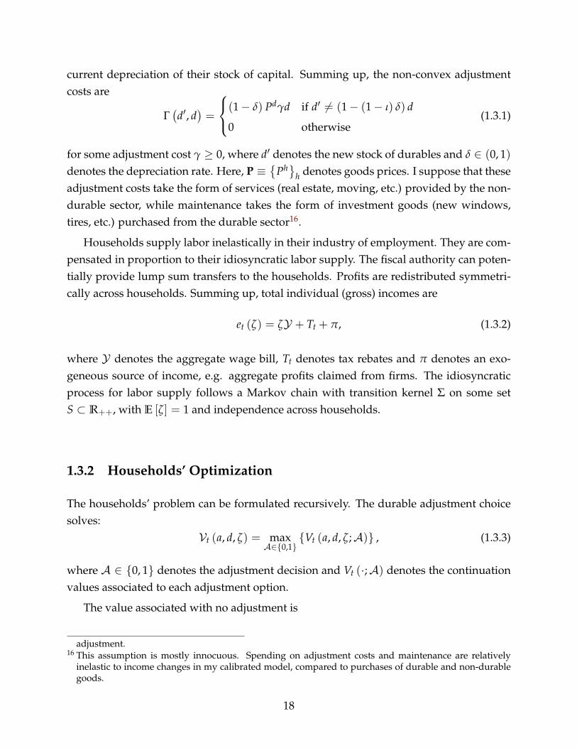
current depreciation of their stock of capital. Summing up, the non-convex adjustmentcosts are

Γ(d′, d

)=

(1 − δ) Pdγd if d′ = (1 − (1 − ι) δ) d

0 otherwise(1.3.1)

for some adjustment cost γ ≥ 0, where d′ denotes the new stock of durables and δ ∈ (0, 1)denotes the depreciation rate. Here, P ≡

Ph

h denotes goods prices. I suppose that theseadjustment costs take the form of services (real estate, moving, etc.) provided by the non-durable sector, while maintenance takes the form of investment goods (new windows,tires, etc.) purchased from the durable sector16.

Households supply labor inelastically in their industry of employment. They are com-pensated in proportion to their idiosyncratic labor supply. The fiscal authority can poten-tially provide lump sum transfers to the households. Profits are redistributed symmetri-cally across households. Summing up, total individual (gross) incomes are

et (ζ) = ζ𝒴 + Tt + π, (1.3.2)

where 𝒴 denotes the aggregate wage bill, Tt denotes tax rebates and π denotes an exo-geneous source of income, e.g. aggregate profits claimed from firms. The idiosyncraticprocess for labor supply follows a Markov chain with transition kernel Σ on some setS ⊂ R++, with E [ζ] = 1 and independence across households.

1.3.2 Households’ Optimization

The households’ problem can be formulated recursively. The durable adjustment choicesolves:

𝒱t (a, d, ζ) = max𝒜∈0,1

Vt (a, d, ζ;𝒜) , (1.3.3)

where 𝒜 ∈ 0, 1 denotes the adjustment decision and Vt (·;𝒜) denotes the continuationvalues associated to each adjustment option.

The value associated with no adjustment is

adjustment.16 This assumption is mostly innocuous. Spending on adjustment costs and maintenance are relatively

inelastic to income changes in my calibrated model, compared to purchases of durable and non-durablegoods.

18

Vt (a, d, ζ; 0) = maxc,a′

u (c, d?)1−σ

1 − σ+ βEt

[𝒱t+1

(a′, d?, ζ ′

)∣∣ ζ]

(1.3.4)

s.t. Pcc + Pdιδ

1 − (1 − ι) δd? + a′ ≤ (1 − τ) et (ζ) + (1 + r) a

a′ ≥ 0,

with d? ≡ (1 − (1 − ι) δ) d. Here, et (ζ) denotes labor income, and r denotes the nominalinterest rate, and τ denotes the tax rate on total income.

Similarly, the value associated with adjustment is

Vt (a, d, ζ; 1) = maxc,a′,d′

u (c, d′)1−σ

1 − σ+ βEt

[𝒱t+1

(a′, d′, ζ ′

)∣∣ ζ]

(1.3.5)

s.t. Pct c + Pd

t(d′ − (1 − δ) d

)+ Γ

(d′, d

)+ a′

≤ (1 − τ) et (ζ) + (1 + r) a

a′ ≥ 0

1.4 Non-Linear Response to Income Shocks

I introduced a canonical model of lumpy durable demand with incomplete markets inthe previous section. Durable adjustment is infrequent and discontinuous in this model.I am interested in the aggregate implications of these microeconomic discontinuities. InSection 1.4.1, I explore how lumpy adjustment at the micro level shapes non-linearities atthe macro level. In particular, I identify the conditions under which this model replicatesthe empirical evidence, by producing an average MPC on durables that increases with thesize of income changes. I discuss various related properties of this model in Section 1.4.2.

1.4.1 Lumpy Investment and Aggregate Non-Linearity

I assume that the economy is initially at its stationary equilibrium.17 I consider an exoge-neous one-time, unanticipated change in aggregate income in period t = 0:

𝒴0 = (1 + ∆)𝒴17 State-contingency is an intrinsic property of models of lumpy investment (Bachmann et al. (2013); Berger

and Vavra (2015); Winberry (2019)). Responses to aggregate shocks are typically larger following an ex-pansion, compared to a contraction. See Section 1.6.4 for a discussion of the connection between state-contingency and non-linearity, and the interaction between redistribution and state-contingency.

19

for some ∆ ∈ R, where 𝒴 denotes the aggregate wage bill at the stationary equilibrium.My focus is on the non-linearity of aggregate investment with respect to the size and signof this income shock.

Aggregate durable investment in the first period as a function of the aggregate incomeshock is18

I (∆) ≡∫

𝒜 (a, d, ζ)︸︷︷︸Hazard

· (d? (a, d, ζ)− (1 − δ) d)︸︷︷︸Gap to target

dΛ (a − ζ∆𝒴 , d, ζ)︸︷︷︸Density

+∫

[1 −𝒜 (a, d, ζ)] ιδd︸︷︷︸Maintenance

dΛ (a − ζ∆𝒴 , d, ζ) , (1.4.1)

where 𝒜 (·) denotes the durable adjustment hazard and d? (·) denotes the adjustmenttarget that solves (1.3.5). The first integral in (1.4.1) captures investment by householdswho pay the fixed adjustment cost, while the second integral captures maintenance bythose who do not.

The model described in Section 1.3 generates a standard inaction region for durable ad-justment. That is, the adjustment hazard takes the form of a step function. In my calibratedmodel, upward adjustment is the most relevant margin at the stationary distribution.19 Ifocus on this case for illustration. The adjustment hazard satisfies

𝒜 (a, d, ζ) =

1 if a ≥ a (d, ζ)

0 otherwise(1.4.2)

for some threshold a (·) that depends on durable holdings and idiosyncratic labor supply.

I am interested in the non-linear properties of the impulse response of aggregate durableinvestment to an income shock:20

I (∆) ≡ I (∆)ℐ − 1, (1.4.3)

where ℐ denotes aggregate investment at the stationary equilibrium.

Fixing the adjustment hazard, the impulse response given by (1.4.1) and (1.4.3) is de-

18 The integration is over the idiosyncratic states (a, d, ζ).19 Downward changes account for roughly 1% of adjustments at the stationary equilibrium. They could

potentially play a more important role in the presence of deleveraging shocks (Guerrieri and Lorenzoni(2017)).

20 In the context of price setting, Caballero and Engel (2007) show that the aggregate response in the Caplinand Spulber (1987) model coincides with the average response across time at the firm-level, when theeconomy is stationary. In other words, my exercise captures the “average” degree of non-linearity overtime in the household-level response of durable investment.

20

termined by adjustment along two margins: the extensive margin, i.e. the households’marginal propensity to adjust; and the intensive margin, i.e. their marginal propensityto invest conditional on adjustment. The following result decomposes the response ofdurable investment into these two margins. For the sake of exposition, I assume thatthe adjustment target d? (·, d, ζ) is smooth and increasing, and that the distribution of liq-uid assets conditional on durable holdings and labor supply admits a smooth densitydΛ (a|d, ζ).21 I define Λ? ≡ margd,ζΛ. Finally, I consider discrete but plausibly smallshocks.22

Proposition 1. The response of durable investment to a positive income shock ∆ > 0 can bedecomposed as follows:

I (∆) ≡ Σ1 (∆)︸︷︷︸Extensive margin

+ Σ2 (∆)︸︷︷︸Intensive margin

+ ς (∆)︸︷︷︸Residual

(1.4.4)

with

Σ1 (∆) ≡1ℐ∫ [

d (d, ζ)− (1 − δ + ιδ) d] ∫ a(·)

a(·)−ζ∆𝒴dΛ (a|d, ζ)

+ κ (d, ζ)∫ a(·)

a(·)−ζ∆𝒴(a + ζ∆𝒴 − a (d, ζ)) dΛ (a|d, ζ)

dΛ?

Σ2 (∆) ≡1ℐ∫

𝒜 (a, d, ζ) [d? (a + ζ∆𝒴 , d, ζ)− d? (a, d, ζ)] dΛ (a, d, ζ)

for some κ (d, ζ) > 0 and some residual ς (∆) that satisfies lim∆→0ς(∆)

∆ = 0. The analogousdecomposition for a negative income shock ∆ < 0 is provided in Appendix 1.B.

Proof. See Appendix 1.B.

The extensive margin consists of two terms. The first term captures discontinuities atthe microeconomic level. Households who pay the fixed cost adjust their stock by a dis-crete amount.23 In turn, the mass of households who adjust depends on the shape of thedistribution of liquid assets. The second term reflects heterogeneity among householdswho pay the fixed cost after the income shock: those that were initially further away from

21 For expositional purposes, I further assume that the conditional distribution dΛ (·|d, ζ) has full supporton [0, a?] with a? > A ≡ sup(d,ζ) a (d, ζ), so that some households adjust for each (d, ζ).

22 Specifically, I assume that ∆ ∈[− sup(d,ζ)

1ζ

a?−a(d,ζ)𝒴 , inf(d,ζ)

1ζ

a(d,ζ)𝒴]

to avoid cases where either no house-hold, or all households adjust. In the following examples, I assume some monotonicity properties aroundthe durable adjustment threshold. These properties might not hold globally. I assume that ∆ is sufficientsmall so that they apply.

23 See Baumol (1952), Tobin (1956) and Scarf (1960) for seminal contributions the subject.

21

their adjustment threshold invest relatively less when adjusting their stock of durables.The intensive margin captures the decreasing propensity to invest conditional on adjust-ment, due to precautionary savings (Carroll and Kimball (1996); Bertola et al. (2005)). Theresidual plays a negligible role in my numerical simulations.

The following three examples clarify the contribution of each term in (1.4.4) to theimpulse response of aggregate durable investment, and its non-linearity. For illustration,I focus on positive income shocks. The opposite case is symmetric. I collect all derivationsin Appendix 1.B.4.

Example 1 (Extensive Margin I). I first focus on adjustment at the extensive margin.Specifically, I illustrate the role of the shape of the distribution of liquid assets, i.e. thefirst term in Σ1 (∆). I suppose that the adjustment target d? (·) is constant at some leveld > 0.24 In this case, there is no adjustment at the intensive margin, households adjust toa common level, and the residual is zero:

Σ2 (∆) = 0 , κ (d, ζ) = 0 and ς (∆) = 0

The impulse response (1.4.4) satisfies

I (∆) =1ℐ∫ [

d (d, ζ)− (1 − δ + ιδ) d] ∫ a(·)

a(·)−ζ∆𝒴dΛ (a|d, ζ) dΛ? (1.4.5)

The response of durable investment depends on the slope of the density of liquid as-sets around the thresholds. If dΛ (·|d, ζ) is uniform, then I (·) is linear in the size of theshock: there is neither amplification, nor dampening. Quantitatively, the relevant caseis one where this density is decreasing around the thresholds (Section 1.6.1). Then, theimpulse response of aggregate durable investment I (·) is convex: more and more house-holds exit their inaction region for expansionary shocks; less and less do so for contrac-tionary shocks. In other words, positive income shocks are amplified as their size increases,and negative shocks are dampened. That is, the impulse response of aggregate durable in-vestment I (∆) is convex in the income shock.

Figure 1.4.1 illustrates this non-linear amplification. The left panel depicts durable in-vestment at the individual level (in blue), and the distribution of liquid assets (in red),25,26

together with the durable adjustment threshold a (d, ζ). I implicitly fix some level of

24 That is, the durable adjustment cost satisfies Γt (d′, d) = 1d′=dγ + (1 − 1d′=d)M with M → +∞.25 The borrowing constraint a ≥ 0 acts as a reflection barrier. Hence the mass at a = 0.26 The model is set in discrete time. Therefore, there is a positive mass of households at the stationary

equilibrium outside of the inaction region. These households adjust in the current period, which depletestheir stock of liquid assets. I discuss the role of discrete time at the end of this section.

22

durable holdings and labor supply. A positive income shock ∆ > 0 shifts the densityof cash-on-hand to the right, as shown in the right panel. When the density of liquid as-sets is decreasing at the adjustment threshold, positive income shocks are amplified: moreand more households adjust at the extensive margin. The opposite happens for negativeshocks.

Figure 1.4.1: Extensive Margin I

Lumpy Adjustment

Adjustment

a (d, ζ)

dΛ

d′ (·)− (1− δ) d

a

Amplification

a (d, ζ)

d′ (·)− (1− δ) d

dΛ dΛ′′

dΛ′

Amplification

a

Example 2 (Extensive Margin II). I focus again on adjustment at the extensive margin, butI now highlight the role of the adjustment target. For illustration, I assume that the ad-justment target d? (·) is linear, with κ (d, ζ) denoting the corresponding slope. To abstractfrom the effect illustrated in the previous example, I suppose that the density dΛ (a|d, ζ)

is uniform over [0, a?] with a (·) < a? < +∞. In this case, adjustment at the intensivemargin is linear, and the residual is zero: ς (∆) = 0. The impulse response (1.4.4) satisfies

I (∆) = θ∆ +

[12

1ℐ

1a?

∫κ (d, ζ) (ζ𝒴)2 dΛ?

]∆2 (1.4.6)

for some θ > 0. Again, this form of adjustment at the extensive margin contributes to aconvex impulse response of aggregate durable investment I (·).

Figure 1.4.2 illustrates this case. As in the previous example, the left panel depictsdurable investment at the individual level (in blue), and the distribution of liquid assets(in red), and the durable adjustment threshold. A positive income shock ∆ > 0 shifts thedensity of cash-on-hand to the right, as shown in the right panel. Positive income shocksare amplified as their size increases: households who decide to adjust do so increasingamounts. On the contrary, the effect of negative shocks is dampened as their magnitudeincreases.

23

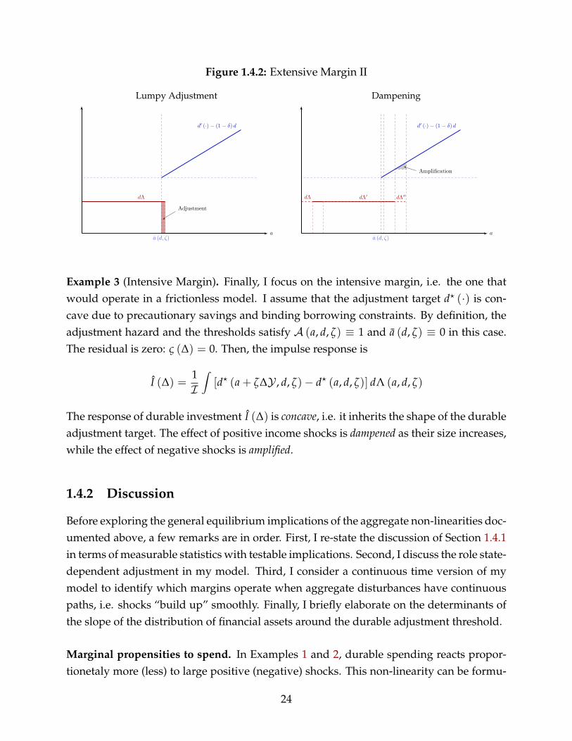
Figure 1.4.2: Extensive Margin II

Lumpy Adjustment

Adjustment

a (d, ζ)

dΛ

d′ (·)− (1− δ) d

a

Dampening

Amplification

a (d, ζ)

dΛ dΛ′ dΛ′′

d′ (·)− (1− δ) d

a

Example 3 (Intensive Margin). Finally, I focus on the intensive margin, i.e. the one thatwould operate in a frictionless model. I assume that the adjustment target d? (·) is con-cave due to precautionary savings and binding borrowing constraints. By definition, theadjustment hazard and the thresholds satisfy 𝒜 (a, d, ζ) ≡ 1 and a (d, ζ) ≡ 0 in this case.The residual is zero: ς (∆) = 0. Then, the impulse response is

I (∆) =1ℐ∫

[d? (a + ζ∆𝒴 , d, ζ)− d? (a, d, ζ)] dΛ (a, d, ζ)

The response of durable investment I (∆) is concave, i.e. it inherits the shape of the durableadjustment target. The effect of positive income shocks is dampened as their size increases,while the effect of negative shocks is amplified.

1.4.2 Discussion

Before exploring the general equilibrium implications of the aggregate non-linearities doc-umented above, a few remarks are in order. First, I re-state the discussion of Section 1.4.1in terms of measurable statistics with testable implications. Second, I discuss the role state-dependent adjustment in my model. Third, I consider a continuous time version of mymodel to identify which margins operate when aggregate disturbances have continuouspaths, i.e. shocks “build up” smoothly. Finally, I briefly elaborate on the determinants ofthe slope of the distribution of financial assets around the durable adjustment threshold.

Marginal propensities to spend. In Examples 1 and 2, durable spending reacts propor-tionetaly more (less) to large positive (negative) shocks. This non-linearity can be formu-

24

lated in terms of observable statistics. Specifically, let

MPCd(∆) ≡

∫∂

∂∆[d′

0(a + ζ∆𝒴 , d, ζ)− (1 − δ) d

]dΛ0

=d

d∆ℐ (∆) (1.4.7)

i.e. the average marginal propensity to spend (MPC) on durable goods.27 In Examples1 and 2, ℐ (·) is convex in income changes ∆. As a consequence, the average MPC ondurable goods increases with income changes. As discussed in Section 1.2, this property isconsistent with the evidence on the consumption response to tax rebates.

Time-dependent adjustment. Durable adjustment is lumpy and state-dependent (i.e. theadjustment hazard is endogeneous) in my model.28 This property plays a central role inthe non-linear response of durable spending in my setting. In models with frictionless ortime-dependent adjustment (à la Calvo (1983)), or even purely non-durable consumption,only the intensive margin operates. In this case, the average MPC decreases with incomechanges due to precautionary savings, as illustrated in Example 3. I elaborate on this pointin Appendix 1.B.2. The relative importance of these two effects, and the effective degreeof non-linearity are quantitative questions. In Section 1.6, I use my calibrated model toimplement the decomposition from Proposition 1. I find that adjustment at the extensivemargin dominates. That is, the average MPC on durables increases with income changes.

Continuous time. My model is set in discrete time, following Berger and Vavra (2015).29

In Appendix 1.B.3, I present a continuous time variant of my model where aggregatedisturbances have continuous paths, i.e. shocks “build up” smoothly. This allows me toclarify the nature of the comparative statics in discrete time, and to identify which of themargins identified in Section 1.4.1 are specific to this comparative statics.

27 Note that (1.4.7) corresponds to the average MPC on durables in each sector, which differs from individualMPCs. Individual MPC are not well-defined at the adjustment threshold (1.4.2).

28 See Alvarez et al. (2017a) for a formal definition of state- and time-dependent adjustment.29 Historically, the literature has favored continuous time models and adopted a more reduced form ap-

proach. Durables were the only explicit state variable, and the evolution of their stock absent adjustmentwas specified exogeneously. See Bertola and Caballero (1990) for a review of this approach. A morerecent strand of the literature has modelled jointly durables and financial assets accumulaton subject touninsured idiosyncratic shocks. Most of these models are set in discrete time, including Berger and Vavra(2015) in the context of durables, Wong (2019) and Kaplan et al. (2017) in the context of housing, and Bach-mann et al. (2013) and Winberry (2019) in the context of capital investment. Exceptions include Achdouet al. (2017) (extensions) and McKay and Wieland (2019).

25

Under the assumptions of Appendix 1.B.3, the flow of durable spending satisfies

it = (s + m∆)Ω0︸︷︷︸Impact

− µ (s + m∆)2 (exp (δt)− 1)Ω1︸︷︷︸Endogeneous distribution

(1.4.8)

for some Ω0, Ω1 > 0. Here, s, m ≥ 0 control the savings rate, ∆ denotes the (flow) incomeshock and µ denotes the slope of the density of the (conditional) stationary distributionof financial assets. Durable spending is given by two terms. The first one captures thefirst order impact of income changes: the larger the income shock, the larger the flowof households who exit their inaction region on impact (t = 0). This term is linear inthe size of the income shock. The second term captures the endogeneous response of thedistribution of financial assets: the larger the income shock, the higher the stock of savingsas time passes. When the slope of the density µ is negative, the flow of households whoexit their inaction region increases over time. Consequently, this second term is non-linearin the size of the income shock, and operates for t > 0. This non-linear mechanism is thecounterpart of the one discussed in discrte time (Example 1). The only difference is that itoperates on impact (t = 0) in discrete time, but takes time to build up in continuous time.Indeed, an income shock in discrete time is akin to an increase in ∆ over a discrete interval[0, t] in continuous time.

It should be noted that the continuous and discrete time cases differ in one importantrespect. The terms Ω0, Ω1 (Appendix 1.B.2) do not depend on the adjustment thresholdd? (·, d) for a > d since households never effectively exit their inaction region in continu-ous time. In Section 1.6.1, I implement numerically the decomposition from Proposition 1.Not surprisingly, I find that the terms involving κ (d, ζ) and Σ2 (∆), and the residual ς (∆)are small quantitatively. Instead, the extensive margin (setting κ (d, ζ) = 0) dominates.

Shape of the density dΛ (·, d). The analysis of Section 1.4.1 identified a key role for theslope of the density of financial assets Λ (·|d, ζ) around that adjustment threshold a (d, ζ).Due to the importance of this object, I briefly elaborate on the determinants on this shape.For tractability, I build on the continuous time version of my model (Appendix 1.B.3).

Since I focus on the properties of the stationary distribution, I temporarily abstractfrom aggregate income shocks. The process for idiosyncratic states (a, D)30 is defined by:

30 In the following, I denote durable holdings by D instead of d to avoid any confusion with differentialoperators or integrands.

26

(i) a law of motion conditional on no adjustment,31,32

da (t) = s (a (t) , D (t) , ζ (t)) dt (1.4.9)

dD (t) = −δD (t) dt (1.4.10)

for some savings function s (·); (ii) an increasing adjustment threshold a (D) of the form(1.4.2); and (iii) an adjustment target d? (·) for durables. Financial assets after adjustmentsatisfy the following budget constraint

a (t) = a (D)− Pd [d? (D)− D] (1.4.11)

For illustration, I assume that the adjustment target d? (·) is constant at some level d > 0,as in Example 1. Idiosyncratic income exp (ζ (t)) follows some diffusion process.

I am interested in the shape of the stationary distribution implied by the process de-scribed above. To gain some insights, I consider an initial distribution of idiosyncraticstates Λ that is uniform on 𝒮 ≡ (a, d) |a ≤ a (d), and I track its evolution over timewhile it converges to the stationary distribution. For illustration, I assume that the sav-ings rate satisfies

s (a, D, ζ) = s + m exp (ζ) (1.4.12)

for some s, m > 0, i.e. households have a constant propensity to save out of transitory in-come shocks. I proceed heuristically in the text to keep the exposition brief. The evolutionof this distribution is characterized more formally in Appendix 1.B.3.

The left panel of Figure 1.4.3 corresponds to the phase diagram associated to (1.4.9)-(1.4.10). Consider households who adjust over the interval [0, t0] with t0 infinitesimallysmall. By assumption, these households share a common durable adjustment target d > 0.They deplete their stock of financial assets (black arrow). After adjustment, householdsaccumulate financial assets. I plot two possible paths associated to different realizations ofthe process ζtt≥0 (red curves). Eventually, households hit again the adjustment thresh-old a (·) (blue line).

The right panel of Figure 1.4.3 depicts the evolution over time of two objects: the distri-bution of financial assets conditional on dt = exp (−δt) d and having adjusted over [0, t0];and the adjustment threshold at ≡ a

(exp (−δt) d

). In period t = t0, this distribution is

31 I abstract from mass points at the borrowing constraint, by assuming below that savings are strictly posi-tive.

32 For simplicity, I abstract from maintenance (ι = 0), and I assume that income shocks are independentover time.

27

uniform over [0, a] with a ≡ supd a (d)− Pd (d − d), using (1.4.11) and by uniformity of

the stationary distribution Λ. I consider two periods t1 and t2 with t0 < t1 < t2. Themean and the variance of the distribution increase with time, from (1.4.9)–(1.4.10) and(1.4.12). On the contrary, the adjustment threshold decreases over time, since a (·) is in-creasing, by assumption. At the top of the distribution of durables, i.e. for t small, theslope of the density is decreasing at the adjustment threshold, and the distance betweenthe durable adjustment threshold at and the mode of the conditional distribution is large.As t increases, this distance shrinks.33,34

Figure 1.4.3: Density at the Adjustment Threshold

Phase Diagram

d⋆

at0 a0

dt1

dt2

a (d)

a

d

Distribution of Financial Assets

at0at1at2

dΛt0

a

dΛt1

dΛt2

a

The predictions of my richer quantitative model are in-line with those described above(see Section 1.6.1). In particular, I document that: (i) the density of financial assets isdecreasing around the adjustment threshold; but (ii) the distance between the adjustmentthreshold and the mode of the distribution is smaller at the bottom of the distribution ofdurable holdings.

1.5 Calibration

The remainder of the paper quantifies the mechanisms documented in Section 1.4. I firstparametrize the model using a mix of external and internal calibration. Following Bergerand Vavra (2015), I adopt a broad definition of durable goods that includes residential

33 In theory, this distance could potentially become negative for sufficiently low holdings of durable hold-ings, i.e. the slope of the density could become positive. In my calibrated model, I find this to be the caseonly for a negligible share of households.

34 In particular, the speed at which the threshold moves closer to the mode of the distribution is controlledby the savings rate, the durable depreciation rate, and the slope of the adjustment threshold.

28

investment and consumer durables. The calibration strategy follows Zorzi (2020a), so I donot discuss it here for concision. Table 1.5.1 describes the resulting parametrization.

1.6 Lumpy Investment and Non-Linearity

In this section, I assess the degree of aggregate non-linearities produced by my struc-tural model. In Section 1.6.1, I implement the decomposition from Proposition 1 in mycalibrated model. In Section 1.6.2, I quantify this non-linearity by simulating the partialequilibrium response of durable spending to persistent income shocks. In Section 1.6.3, Icompare the resulting magnitudes with their empirical counterparts. Finally, I relate myfindings to the literature on state-contingent responses with lumpy adjustment in Section1.6.4.

1.6.1 Decomposition

I start by examining the two sources of aggregate non-linearities identified in Section 1.4.1:the extensive and intensive margins of durable adjustment. Specifically, I implement thedecomposition from Proposition 1 for a one-time, transitory shock ∆.35

Figure 1.6.1 plots each of the three objects in (1.4.4) and (1.B.1). The total response(i.e. the sum of these three components) is non-linear: expansionary shocks are ampli-fied as the size of the shock increases, while contractionary shocks are dampened. Thatis, the average MPC on durables increases with income changes. Adjustment at the ex-tensive margin dominates quantitatively, and entirely accounts for this non-linear effect.36

In other words, lumpy and state-contingent adjustment is responsible for this aggregatenon-linearity, while precautionary savings plays a minor role. Figure 1.A.1 in Appendix1.A.2 further decomposes the extensive margin of adjustment into each of the two termsin Σ1 (∆). Consistently with the discussion on continuous time (Section 1.4.2), I find thatthe term capturing changes in the size of durable purchases conditional on adjustment isquantitatively small. However, it accounts for a non-negligible share of the non-linearityin the response of durable spending for expansionary shocks.

As illustrated by Examples 1 and 2, the extensive margin of adjustment is controlledby two objects: the slope of the density of the distribution of liquid assets around theadjustment thresholds; and the slope of the durable adjustment target. In turn, the in-tensive margin is shaped by the concavity of the durable investment target. Figure 1.A.2

35 This transitory shock is annualized with a persistence that delivers a half-life of 6 quarters.36 This prediction is in-line with the findings of Fuster et al. (2018).

29

Table 1.5.1: Calibration

Parameter Description Calibration Source / Target

Preferencesβ Discount factor 0.985 Internal calibrationν Elasticity of substitution 1 See textϑ Non-durable parameter 0.731 Internal calibrationσ EIS (inverse) 4 See textε Elasticity of substitution (inverse) 10 Kaplan et al. (2018)

Durable goodsδ Depreciation rate 0.018 Berger and Vavra (2015)γ Adjustment cost 0.025 Internal calibrationι Maintenance parameter 0.5 See text

Income processρ Persistence 0.967 Floden and Lindé (2001)σ Standard deviation 0.13 Floden and Lindé (2001)

LiquidityB Ratio of bond supply to GDP 1.490 Internal calibration

Labor supplyµd Mass of households (durable) 0.187 CES

ProductionAd Relative productivity (durable) 0.490 Internal calibrationα Decreasing returns 0.3 Berger and Vavra (2015)

Prices and policyλ Calvo parameter 1 See textϕ Taylor rule coefficient (inflation) 1.25 Kaplan et al. (2018)

30

(Appendix 1.A.2) plots these objects for various percentiles of the distribution of durablegoods (fixing idiosyncratic labor supply at its median level). The density of liquid assets istypically decreasing around the adjustment threshold and the durable adjustment target isincreasing but concave. As anticipated in Section 1.4.2, the adjustment threshold gets closerto the mode of the distribution of liquid assets as the stock of durables decreases.

Figure 1.6.1: Decomposition from Proposition 1

Contraction Expansion

Extensive Σ1 (·) /ℐ Intensive Σ2 (·) /ℐ Residual ς (·) /ℐ

1.6.2 Persistent Income Shocks

I now consider the effect of an aggregate, persistent income shock. I abstract from redistri-bution for now. The wage bills satisfy: 𝒴h

t /𝒴h = t, with t = ψ0ρt for some persistenceρ ∈ (0, 1). I am interested in the non-linear properties of the aggregate response of durablespending as I vary ψ0. I set ρ to obtain a half-life of 6 quarters and replicate the behaviorof real filtered GDP since 1960.

Impulse responses. Figures 1.6.2 and 1.6.3 plot the cumulative response of spending over4 quarters in terms of ψ0, for expansionary and contractionary shocks.37,38 The left panelscorrespond to durable investment, and the right panels to non-durable consumption. Thedashed lines extrapolate the response associated to ψ0 = −0.01 and ψ0 = 0.01, respec-tively.

37 I choose a horizon of 4 quarters for two reasons. First, the spending response to persistent income changesis typically hump-shaped in my calibration as discussed at the end of this section. A sufficiently longtime horizon captures this delayed response. Second, averaging out over a longer horizons smoothes theimpulse responses. The cumulative responses over two or more years are very similar.

38 I annualize these cumulative responses by diving them by the number of quarters over which I cumulate.

31

I find that the response of durable spending to positive income shocks is amplifiedas their size increases. On the contrary, this response is dampened for negative incomeshocks. That is, durable spending is convex in income changes. This effect is economi-cally significant. For instance, consider shocks of the magnitude experienced by durableworkers during the Great Recession, i.e. a 10% persistent income change. Fixing thismagnitude, the average MPC on durables is roughly 25% higher for expansionary shocks,compared to contractionary shocks. The response of non-durable consumption contrastssharply with that of durable investment. Expansionary shocks are dampened due to pre-cautionary savings, and contractionary shocks are amplified. In other words, lumpy andstate-dependent durable adjustment not only undoes the effect of precautionary savings,but it also predicts that non-linearities actually operate in the opposite direction.

Timing. The analysis of Section 1.4 assumed that income shocks were fully transitory.Households are non-Ricardian in my model due to borrowing constraints, so the timingof income shocks is actually relevant and affects the profile of the impulse response. Inparticular, the degree of non-linearity needs not be uniform over time. Figures 1.6.2 and1.6.3 effectively obscure these dynamic considerations by aggregating over a sufficientlylong time horizon. Figure 1.A.4 in Appendix 1.A.2 plots the dynamic impulse responsesof durable spending to (positive) income shocks of various sizes. These impulse responsesare normalized by the size of these shocks. A clear pattern emerges: as the size of incomeshocks gets larger, the normalized impulse response increases on impact, and becomesmore persistent. However, it typically decreases for a few quarters in the medium term,as households accumulate savings to finance larger purchases in the following periods.The cumulative response of durable spending increases with the size of income shocks.39

That is, the average MPC on durables increases on impact and in the longer-term with thesize of income changes, but decreases in the medium-term. Put it differently, the impulseresponse of durable spending (in level) is convex on impact and in the longer run, butconcave for a few quarters after the shock.

39 Note that the cumulative response of spending would necessarily be linear (for sufficiently long horizons)in the size of income shocks if households consumed a single good. Indeed, the increase in income iseventually spent. This need not be the case with multiple goods, as in my setting.

32

Figure 1.6.2: Impulse Response (4 quarters) – Contraction

Durables Non-Durables

Figure 1.6.3: Impulse Response (4 quarters) – Expansion

Durables Non-Durables

33

Figure 1.6.4: Persistent Income Shocks – Timing

Impulse Response

t0 t1 t2

∆0∆1 > ∆0

MPCd

t (·) ↑MPC

d

t (·) ↓

t

It (∆) /∆

For reference, Figure 1.6.4 schematizes this pattern and depicts the impulse response ofdurable investment I (∆) normalized by the size of the income change ∆ for two possiblevalues of this shock. The timing of the impulse response depends on the magnitude of theshock.

1.6.3 Magnitudes

In the previous sections, I confirmed that a canonical model of lumpy durable demandwith incomplete markets produces the correct form of non-linearity: the average MPC ondurables increases with the size of income changes. I now assess the importance of thisnon-linearity by comparing it to the empirical evidence. I then suggest avenues to im-prove the quantitative properties of the model.

Magnitudes. To assess the performance of the model, I compare the degree of non-linerityit produces with the one estimated by Fuster et al. (2018). Specifically, I conduct the sameexperiment as theirs using my model, by computing the average MPC on durables out ofunanticipated, transitory income changes of the various sizes.40 Table 1.6.1 reports theseaverage MPCs. For comparison, I normalize the average MPC out of a $500 tax rebate to1 in the data and in my model.41 Not surprisingly, the model produces the correct form of

40 Following Kaplan et al. (2018), I assume that the average quarterly labor income is $16, 500.41 The average MPC on durables out of a $500 rebate is 19.4% in my model, while Fuster et al. (2018) obtain

34

non-linearity. However, the magnitudes are substantially lower than those observed in thedata. Comparing a $5, 000 rebate to a $500 rebate, the average MPC on durables increasesroughly by 150% in the data, but only by 30% in the model. That is, this canonical modelpredicts non-linearities that are substantially smaller than those observed in the data.

Table 1.6.1: Average Marginal Propensities to Spend on Durables (1 quarter)

Amount $500 $2, 500 $5, 000

Fuster et al. (2018) 100% 189% 263%

Model 100% 117% 131%

Taking stock. In ongoing work (Zorzi (2020b)), I develop a richer model of lumpy durabledurable to improve its quantitative performance and better match the degree of non-linearity observed in the data. This richer model differs from the canonical model used inthis paper in three respects.

First, I allow households to invest in multiple durable goods (consumer durables, ve-hicles and housing). This generalization is not only more realistic empirically. It also ad-dresses a key shortcoming of the canonical model of lumpy durable demand that I use inthis paper. By pooling all durable goods, this model requires that households pay a fixedcost (1.3.1) that is proportional to the nominal value of their entire stock of durables when-ever they adjust this stock. The resulting fixed cost might be prohibitively high for thepurchase of small- or medium-size durables. The evidence of Parker et al. (2013) suggeststhat vehicle purchases (medium-sized goods) are responsible for most of the non-linearityin durable demand. An excessively high fixed cost could artificially dampen the degreeof non-linearity in the model. Figure 1.A.2 in Appendix 1.A.2 illustrates this point. Whenfacing a high fixed cost of adjustment, households wait until they have accumulated largesavings in financial assets before they adjust their stock of durables. Under a realistic cal-ibration for the income process, the right tail of the distribution of financial assets flattensprogressively. This effectively mutes the extensive margin of adjustment, which is themain source of non-linearity in my model (Sections 1.4.1 and 1.6.1).

Second, I introduce convex adjustment costs for financial assets. This addition servestwo purposes. It allows to better match the average MPC on non-durables (Kaplan et al.(2018)). And it strenghtens the degree of non-linearity in the response of durable spend-ing, by lowering the marginal benefit of savings for larger income shocks.

a response of 3.9%. Again, their estimates lie at the lower end of those obtained in the literature.

35

Finally, I suppose that households face observation costs (Bonomo et al. (2010); Al-varez et al. (2011, 2016)) on top of non-convex adjustment costs for durables. This fea-ture effectively introduces a degree of time-dependency (Section 1.4.2) in the adjustmentof durables. In itself, this addition reduces the degree of non-linearity produced by themodel (Alvarez et al. (2018)). However, it helps address two another pathological proper-ties of the canonical model I am using: the response of durable spending to income shocksis not sufficiently persistent; and the elasticity of durable spending to changes in the usercost is excessively high (House (2014); Winberry (2019); McKay and Wieland (2019)).

1.6.4 State-Contingency

I conclude this section by drawing a connection between the non-linearity that I focus on,and another property of models of lumpy adjustment: state-contingency.

Using a version of the income fluctuations problem (1.3.3)–(1.3.5) with aggregate risk,Berger and Vavra (2015) find that the response of durable investment to (income) changesis pro-cylical, i.e. the effect of shocks is amplified during expansions compared to con-tractions. For illustration, I compute the response of aggregate investment to a one-time,transitory income shock following a period of expansion or contraction. The initial boomor bust results from a persistent, unanticipated income change. Specifically, aggregate in-comes satisfy 𝒴t/𝒴 = t, with t = ψ0ρt. The persistence ρ calibrated as in Section 1.6.2,and I vary the initial income shock ψ0. A transitory, unanticipated income shock takesplace after 6 quarters. It takes the form of an exogeneous $1, 000 transfer, i.e. the aver-age 2008 stimulus payment. Table 1.6.2 reports the average (cumulative) MPC on durablegoods over a year, for various magnitudes of the initial expansion or recession (ψ0).42 Thecumulative response of aggregate durable spending is larger after a boom than a bust. Theeffect is relatively small in this example however, since the income shock is fully transitory,i.e. the present discounted value of income changes is small.

Table 1.6.2: Average Marginal Propensity to Spend on Durables (4 quarters)

Initial state (ψ0) −4% −2% 0% 2% 4%

Average MPC ($1, 000) 0.2192 0.2225 0.2265 0.2292 0.2319

I now argue that this state-contingent amplification can be understood as a manifes-tation of the form of non-linearity that I am interested in. For expositional purposes, I42 It should be noted that average MPCs on durables is substantially smaller in my model (Table 1.6.2), than

in the data (Table 1.2.1).

36

suppose there is a single source of aggregate disturbance ξtt, which follows a Markovprocess of order 1. I am interested in the impulse response of aggregate durable invest-ment, conditional on the state of the economy. Specifically, this response is parametrizedby two aggregate states: the exogeneous disturbance (ξt) and the distribution of idiosyn-cratic states (Λt). The impulse response to an innovation z in ξt in period t is

ℛ (z; ξt, Λt) = ℐ (ξt + z, Λt)− ℐ (ξt, Λt) , (1.6.1)

where ℐ (·) denotes aggregate durable investment (1.4.1). In the context of Section 1.6.2,ξtt corresponds to a persistent sequence of transfers. In this case, the impulse responseℛ (·) corresponds to the average MPC on durables following a transitory income shock.

There are three possible sources of state-dependency: the aggregate disturbance ξt

itself; the (marginal) distribution of liquid assets margaΛt; or the (marginal) distributionof durable holdings margdΛt.43 The distribution of durable holdings is unlikely to beresponsible for the pro-cyclicality of the response of durable investment: durable holdingsare already high at the peak of a boom, which should actually mitigate the response ofdurable expenditure. I thus focus on the two other states in the following.

By definition, dependence on the aggregate disturbance ξt corresponds to the non-linearity documented in Figures 1.6.2 and 1.6.3. Holding the distribution of idiosyncraticstates at its stationary level Λ and fixing some innovation z > 0,

ℛ(z; ξ ′t, Λ

)> ℛ (z; ξt, Λ) ∀ξ ′t > ξt ⇐⇒ ℐ (·, Λ) is strictly convex

using (1.6.1).

Similarly, dependence on the (marginal) distribution of financial assets is intrinsicallyrelated to the form of non-linearity I am interested in. I illustrate this point using thecontinuous time version of my model presented in Appendix 1.B.3. Specifically, I aminterested in the response to an (unanticipated) income shock ∆ over an interval [t, t′]with t′ > t > 0 after a sequence of (unanticipated) shocks ∆? over the interval [0, t). Theseinitial shocks shift the distribution of financial assets in period t. Under the assumptionsof Appendix 1.B.3, the flow of durable investment in period t satisfies

it (∆) = (s + m∆)Ω0 − µ (s + m∆) (s + m∆?) (exp (δt)− 1)Ω1 (1.6.2)

for some Ω0, Ω1 > 0. Here, µ denotes the slope of the density of financial assets at the

43 Obviously, the joint distribution Λt is the relevant state variable. I focus on the marginal distributions forthe sake of the argument.

37

adjustment threshold (stationary equilibrium), and s, m ≥ 0 control the savings rate. Inparticular, durable spending (1.6.2) is linear in ∆, but contingent on the size of the initialincome change and the duration over which it occurs (∆?, t). Fixing some horizon t, theimpulse response increases after a period of expansion (∆? > 0), but decreases after aperiod of recession (∆? < 0) whenever the slope µ? is negative (Section 1.6.1).

Note that (1.6.2) coincides with the dynamic impulse response to an income shock(1.4.8) when parametrized with ∆? = ∆. In particular, the degrees of non-linearity andstate-contingency are determined by the same structural objects. The very reason whylarge shocks generate non-linear responses is that they induce changes the distributionof financial assets (Section 1.4.2), i.e. they endogeneously affect the aggregate state. Inother words, the dynamic impulse response to an income shock is non-linear in the sizeof the shock ∆ if and only if the impulse response to a shock at the same horizon exhibitsstate-contingency.

1.7 Conclusion

In this paper, I explore whether a canonical model of lumpy durable investment withincomplete markets can produce an average MPC on durable that increases with the sizeof income changes. I clarify the source of these macro non-linearities analytically, and Iconfirm in numerical exercises that the response of durable investment is non-linear inincome changes. However, I find that the magnitudes are substantially lower than thoseobserved in the data. I suggest various avenues to improve the quantitative performanceof the model.

38

Appendix to Chapter 1

1.A Quantitative Appendix

In this Appendix, I describe the model in more details and I present complementary nu-merical results. Section 1.A.1 describes the full model. Section 1.A.2 presents additionalresults that are not reported in text. The approach used to simulate and calibrate the modelis discussed in Zorzi (2020a).

1.A.1 Environment

For concision, Section 1.3 provided a partial description of the model. For reference, I nowpresent the full model.

Timing. Periods are indexed by t ∈ 0, 1, . . .. There is no aggregate risk. I focus onone-time, unanticipated but persistent shocks. Each period effectively consists of twosub-periods, indexed by t.0 (−) and t.1 (+). Households make their adjustment deci-sions at t.0, and their consumption, saving and investment decisions at t.1. In period t.0,households are indexed by their financial asset holdings (a), their holdings of durablegoods (d) and their idiosyncratic labor supply shock (ζ). In period t.1, households are inaddition indexed by their adjustment choice (𝒜) during the previous sub-period.44 Theconditional distributions of idiosyncratic states within each sector, at the begining of eachsubperiod, are denoted by Λ−

t−1 and Λ+t . All agents have perfect foresight, and all (aggre-

gate) information is revealed at the begining of the first sub-period at t = 0.

Households. The households’ value function in period t.0 satisfies:

𝒱t (a, d, ζ) = max𝒜∈0,1

Vt (a, d, ζ;𝒜) (1.A.1)

44 This additional state variable is for notational convenience. Financial assets are a sufficient statistics forthis adjustment.

39

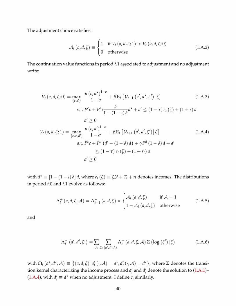
The adjustment choice satisfies:

𝒜t (a, d, ζ) ≡

1 if Vt (a, d, ζ; 1) > Vt (a, d, ζ; 0)

0 otherwise(1.A.2)

The continuation value functions in period t.1 associated to adjustment and no adjustmentwrite:

Vt (a, d, ζ; 0) = maxc,a′

u (c, d?)1−σ

1 − σ+ βEt

[𝒱t+1

(a′, d?, ζ ′

)∣∣ ζ]

(1.A.3)

s.t. Pcc + Pdιδ

1 − (1 − ι) δd? + a′ ≤ (1 − τ) et (ζ) + (1 + r) a

a′ ≥ 0

Vt (a, d, ζ; 1) = maxc,a′,d′

u (c, d′)1−σ

1 − σ+ βEt

[𝒱t+1

(a′, d′, ζ ′

)∣∣ ζ]

(1.A.4)

s.t. Pcc + Pd (d′ − (1 − δ) d)+ γPd (1 − δ) d + a′

≤ (1 − τ) et (ζ) + (1 + rt) a

a′ ≥ 0

with d? ≡ [1 − (1 − ι) δ] d, where et (ζ) ≡ ζ𝒴 + Tt + π denotes incomes. The distributionsin period t.0 and t.1 evolve as follows:

Λ+t (a, d, ζ,𝒜) = Λ−

t−1 (a, d, ζ)×

𝒜t (a, d, ζ) if 𝒜 = 1

1 −𝒜t (a, d, ζ) otherwise(1.A.5)

and

Λ−t(a′, d′, ζ ′

)=∑

𝒜∑

Ωt(a′,d′;𝒜)

Λ+t (a, d, ζ,𝒜)Σ

(log(ζ ′)|ζ)

(1.A.6)

with Ωt (a?, d?;𝒜) ≡ (a, d, ζ) |a′t (·;𝒜) = a?, d′t (·;𝒜) = d?, where Σ denotes the transi-tion kernel characterizing the income process and a′

tand d′

tdenote the solution to (1.A.1)–

(1.A.4), with d′t≡ d? when no adjustment. I define ct similarly.

40

1.A.2 Complementary Numerical Results

I provide below some numerical results that were omitted from the main text.

Extensive margin. In Section 1.6.1, I implement the decomposition from Proposition 1. InFigure 1.A.1, I further decompose the extensive margin of adjustment into the two terms inΣ1 (∆) in (1.4.4) and (1.B.1). I denote by Σ?1 (·) the first term in Σ1 (·), i.e. with κ (d, ζ) = 0.

Figure 1.A.1: Decomposition from Proposition 1

Contraction Expansion

Extensive 1: Σ?1 (·) /ℐ Extensive 2: (Σ1 (·)− Σ?1 (·)) /ℐ

Sources of non-linearities. Figure 1.A.2 plots the density of the distribution of liquidassets (normalized by quarterly GDP) and the durable investment target for various per-centiles of the distribution of durable goods (fixing idiosyncratic labor supply at its me-dian level). The dashed lines denote the durable adjustment thresholds.

41

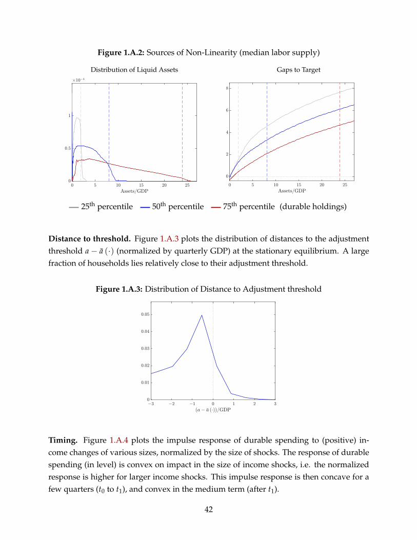
Figure 1.A.2: Sources of Non-Linearity (median labor supply)

Distribution of Liquid Assets Gaps to Target

25th percentile 50th percentile 75th percentile (durable holdings)

Distance to threshold. Figure 1.A.3 plots the distribution of distances to the adjustmentthreshold a − a (·) (normalized by quarterly GDP) at the stationary equilibrium. A largefraction of households lies relatively close to their adjustment threshold.

Figure 1.A.3: Distribution of Distance to Adjustment threshold

Timing. Figure 1.A.4 plots the impulse response of durable spending to (positive) in-come changes of various sizes, normalized by the size of shocks. The response of durablespending (in level) is convex on impact in the size of income shocks, i.e. the normalizedresponse is higher for larger income shocks. This impulse response is then concave for afew quarters (t0 to t1), and convex in the medium term (after t1).

42

Figure 1.A.4: Impulse Responses to Earnings Shocks

∆ = 2% ∆ = 6% ∆ = 10%

1.B Omitted Proofs, Results and Derivations

1.B.1 Decomposition

I provide a decomposition of the response of durable investment in income shocks in Sec-tion 1.4.1. Expression (1.4.4) in Proposition 1 applies to positive income shocks. I firstprovide the analogous decomposition for negative income shocks, before proving theseresults.

Proposition 1 (cont’d). The response of durable investment to a negative income shock∆ < 0 can be decomposed as follows:

I (∆) ≡ Σ′1 (∆)︸︷︷︸

Extensive margin

+ Σ′2 (∆)︸︷︷︸

Intensive margin

+ ς′ (∆)︸︷︷︸Residual

(1.B.1)

with

Σ′1 (∆) ≡

1ℐ∫ [

d (d, ζ)− (1 − δ + ιδ) d] ∫ a(·)


+ κ (d, ζ)∫ a(·)

a(·)−ζ∆𝒴(a − a (d, ζ)) dΛ (a|d, ζ)

dΛ?

Σ′2 (∆) ≡

1ℐ∫ ∫ +∞

a(·)−ζ∆𝒴[d? (a + ζ∆𝒴 , d, ζ)− d? (a, d, ζ)] dΛ (a|d, ζ) dΛ?

43

for some κ (d, ζ) > 0 and some residual ς′ (∆) that satisfies lim∆→0ς′(∆)

∆ = 0.

Proof of Proposition 1. From (1.4.1)–(1.4.3),

I (∆) ≡ 1ℐ

[∫ ∫ +∞

a(d,ζ)(d? (a, d, ζ)− (1 − δ) d) dΛ ( a − ζ∆𝒴| d, ζ) dΛ?

+∫ ∫ a(d,ζ)

0δdιdΛ (a − ζ∆𝒴 , d, ζ) dΛ? − ℐ

]where Λ? ≡ margd,ζΛ denotes the marginal distribution of durable holdings and produci-tivty. By definition, aggregate durable investment at the stationary equilibrium satisfies:ℐ ≡ I (0). Thus,

I (∆) ≡ 1ℐ

∫ ∫ +∞

a(d,ζ)(d? (a, d, ζ)− (1 − δ) d) dΛ ( a − ζ∆𝒴| d, ζ)︸︷︷︸

≡Ω1

dΛ?

+∫ ∫ a(d,ζ)

0δdιdΛ ( a − ζ∆𝒴| d, ζ)︸︷︷︸

≡Ω2

dΛ?

(1.B.2)

where Λ ( a − ζ∆𝒴| d, ζ) ≡ Λ ( a − ζ∆𝒴| d, ζ)− Λ ( a| d, ζ), with an abuse of notation.Using the change of variable a′ ≡ a − ζ∆𝒴 , the first term in (1.B.2) is

Ω1 =∫ +∞

a(d,ζ)−ζ∆𝒴(d? (a + ζ∆𝒴 , d, ζ)− (1 − δ) d) dΛ ( a| d, ζ)

−∫ +∞

a(d,ζ)(d? (a, d, ζ)− (1 − δ) d) dΛ ( a| d, ζ)

Then,

Ω1 =∫ +∞

a(d,ζ)(d? (a + ζ∆𝒴 , d, ζ)− d? (a, d, ζ)) dΛ ( a| d, ζ) dΛ?

+∫ a(d,ζ)

a(d,ζ)−ζ∆𝒴(d? (a + ζ∆𝒴 , d, ζ)− (1 − δ) d) dΛ ( a| d, ζ)︸︷︷︸

≡Ω1

(1.B.3)

The first integral in (1.B.3) corresponds to the intensive margin of adjustment in Proposi-tion 1. The second integral contributes to the extensive margin, together with the term Ω2

in (1.B.2).

44

This second integral can be decomposed as follows:

Ω1 =∫ a(d,ζ)

a(d,ζ)−ζ∆𝒴

(d? (a + ζ∆𝒴 , d, ζ)− d (d, ζ)

)dΛ ( a| d, ζ)

+(d (d, ζ)− (1 − δ) d

) ∫ a(d,ζ)

a(d,ζ)−ζ∆𝒴dΛ ( a| d, ζ)

where d (d, ζ) ≡ d? (a (d, ζ) , d, ζ) denotes investment at the threshold. By assumption,d? (·) is smooth. Define κ (d, ζ) ≡ ∂

∂a d? (a, d, ζ)∣∣∣a=a(d,ζ)

> 0. Then,

Ω1 ≡κ (d, ζ)∫ a(d,ζ)

a(d,ζ)−ζ∆𝒴(a + ζ∆𝒴 − a (d, ζ)) dΛ ( a| d, ζ) + ς (∆, d, ζ)

+(d (d, ζ)− (1 − δ) d

) ∫ a(d,ζ)

a(d,ζ)−ζ∆𝒴dΛ ( a| d, ζ) (1.B.4)

where ς (∆, d, ζ) is defined residually.

Again, using a change of variable, the second term in (1.B.2) corresponds to

Ω2 = δdι

[∫ a(d,ζ)−ζ∆𝒴

0dΛ ( a| d, ζ)−

∫ a(d,ζ)

0dΛ ( a| d, ζ)

]= −δdι

∫ a(d,ζ)

a(d,ζ)−ζ∆𝒴dΛ ( a| d, ζ) (1.B.5)

since Λ ( ·| d, ζ) has positive support, from the household’s income fluctuations problem(1.3.4)–(1.3.5).

Note that the previous expressions apply to both positive income shock ∆ > 0 andnegative income shocks ∆ < 0. However, the attribution of each term to the extensive andintensive margins differs between these two cases. I thus treat them separately.

Case 1: ∆ < 0. The expression (1.4.4) in the text follows by collecting the terms from(1.B.2)–(1.B.4) and (1.B.5), and by definition of the hazard (1.4.2) and the marginal distri-bution Λ?. Finally, ς (∆) is a second-order term, by Taylor’s Theorem.

Case 2: ∆ < 0. Note that

Σ2 (∆) =1ℐ∫ ∫ a(·)−ζ∆𝒴

a(·)[d? (a + ζ∆𝒴 , d, ζ)− d? (a, d, ζ)] dΛ ( a| d, ζ)

+∫ +∞

a(·)−ζ∆𝒴[d? (a + ζ∆𝒴 , d, ζ)− d? (a, d, ζ)] dΛ ( a| d, ζ)

dΛ?

45

Equivalently,

Σ2 (∆) =1ℐ∫ ∫ a(·)−ζ∆𝒴

a(·)

[d? (a + ζ∆𝒴 , d, ζ)− d (d, ζ)

]dΛ ( a| d, ζ)

+∫ +∞

a(·)−ζ∆𝒴

[d (d, ζ)− d? (a, d, ζ)

]dΛ ( a| d, ζ)

+∫ +∞


dΛ? (1.B.6)

Then,

Σ2 (∆) =1ℐ∫

κ (d, ζ)∫ a(·)−ζ∆𝒴

a(·)ζ∆𝒴dΛ ( a| d, ζ)

+∫ +∞


dΛ? + ς (∆) (1.B.7)

for some second-order term ς (∆), by definition of κ (d, ζ) and d (d, ζ). Therefore, sum-ming up Σ1 (·) and Σ2 (·) in the expression (1.4.4) in the text:

Σ1 (∆) + Σ2 (∆) =1ℐ∫ [

d (d, ζ)− (1 − δ + ιδ) d] ∫ a(·)


+κ (d, ζ)∫ a(·)

a(·)−ζ∆𝒴(a − a (d, ζ)) dΛ (a|d, ζ)

+∫ +∞


dΛ? + ς (∆)

(1.B.8)

Finally, the expression (1.B.1) is obtained from (1.B.8), collecting the terms appropriately.

1.B.2 Time-Dependent Adjustment

State-dependent (or lumpy) adjustment is key for the the non-linear effect of incomeshocks discussed in Section 1.4.1. To illustrate this point, I consider an alternative for-mulation where adjustment is instead time-dependent à la Calvo (1983).

In this case, the households’ problem is

46

Vht (a, d, ζ; 0) = max

c,a′u (c, d?)1−σ

1 − σ+ βEt

[Vh

t+1(a′, d?, ζ ′;𝒜t+1

)∣∣∣ ζ]

(1.B.9)

s.t. Pct c + Pd

t ιδ

1 − (1 − ι) δd? + a′ ≤ (1 − τt) eh

t (ζ) + (1 + rt−1) a

a′ ≥ 0

with d? ≡ (1 − (1 − ι) δ) d, and


c,a′,d′u (c, d′)1−σ

1 − σ+ βEt

[Vh

t+1(a′, d′, ζ ′;𝒜t+1

)∣∣∣ ζ]

(1.B.10)

s.t. Pct c + Pd

t(d′ − (1 − δ) d

)+ a′

≤(

1 − τht

)eh

t (ζ) + (1 + rt−1) a

a′ ≥ 0

with 𝒜tt≥0 following a Poisson process with intensity θ ∈ [0, 1], with independenceacross households and sectors. Note that the case θ ≡ 1, i.e. frictionless adjustment,coincides with the case Γt (d′, d) ≡ 0 in the original formulation with lumpy adjustment.

Aggregate durable spending in period t = 0 is

ℐ (∆) =θ∫

[d? (a, d, ζ)− (1 − δ) d] dΛ (a − ζ∆𝒴 , d, ζ)

+ (1 − δ) ιδddΛ (a − ζ∆𝒴 , d, ζ) (1.B.11)

where d? (·) solves the problem with adjustment (1.B.10) at t = 0. Thus, the impulseresponse of durable spending is

ℐ (∆) =1ℐ θ

∫[d? (a + ζ∆𝒴 , d, ζ)− d? (a + ζ∆𝒴 , d, ζ)] dΛ (a, d, ζ) (1.B.12)

since ℐ ≡ ℐ (0). Therefore, the impulse response ℐ (·) inherits the shape of durable spend-ing d? (·; d, ζ) as a function of liquid, financial assets.

Figure 1.B.1 plots durable spending d? (·) in terms of financial assets, for various lev-els of durable holdings and fixing productivity at its median level. Durable spending isconcave due to precautionary savings (Carroll and Kimball (1996)). As a result, aggregatedurable spending is concave in income changes. This stands is sharp contrast with thecase of lumpy adjustment, where the durable spending is convex in income changes (see

47

Sections 1.4.1 and 1.6.1).

Figure 1.B.1: Durable Spending - Calvo (median labor supply)

25th percentile 50th percentile 75th percentile (durable holdings)

1.B.3 Continuous Time

My model is set in discrete time. In this appendix, I consider instead a continuous timeversion. To simplify the expressions, I abstract from maintenance and uninsured idiosyn-cratic income risk in the following.

Dynamic system. For the sake of illustration, I assume that income shocks ∆tt≥0 areperceived as transitory, even if I am interested in persistent sequences of income changes.As a consequence, households’ optimal savings policy conditional on no adjustment isgiven by some time-invariant s (a, D, ∆).45 The process for idiosyncratic states (a, D) isdefined by: (i) a law of motion conditional on no adjustment,46

da (t) = s (a (t) , D (t) , ∆ (t)) dt (1.B.13)

dD (t) = −δD (t) dt; (1.B.14)

(ii) an adjustment threshold a (D) of the form (1.4.2); and (iii) an adjustment target d? (D)

for durables.47 Financial assets after adjustment satisfy the following budget constraint

45 In the following, I denote durable holdings by D instead of d to avoid any confusion with differentialoperators or integrands.

46 I abstract from mass points at the borrowing constraint, by assuming that there is no uninsured idiosyn-cratic income risk and that the savings rate is strictly positive (see Assumption 2 below).

47 Formally, a (·) is a jump reflecting barrier, and the adjustment target d? (·) corresponds to the reset pointwhen hitting this barrier. Note that a = a (D) when hitting the barrier, so that d? (·) can be expressed interms of D only.

48

(1.4.11). The economy is initially at its stationary equilibrium. I impose the followingrestrictions to simplify the analysis.

Assumption 1. The adjustment threshold satisfies a (·) = a > 0.

Assumption 2. The savings function satisfies

s (a, D, ∆) = s + m∆ (1.B.15)

for some s > 0 and some m > 0.

Assumption 3. Households who adjust borrow up to their constraint,

d? (D) = D +1

Pd a (D)

The first restriction holds in my (discrete time) calibrated model. The second as-sumption stipulates the households have a constant marginal propensity to spend outof marginal, transitory income changes,48 and that the savings rate does not depend onasset holdings. Finally, the third restriction allows me simplify the expressions when char-acterizing the evolution of the distribution of idiosyncratic states in the interior of thestate-space (a > 0). This restriction also typically holds in my (discrete time) calibratedmodel.

Comparative statics. I consider a sequence of persistent (but unanticipated) income changes.That is, ∆t ≡ ∆ ∈ R for all t ∈ [0, T] and some horizon T > 0.

Investment. Cumulative aggregate durable investment satisfies49

ℐ(t′)− ℐ (t) ≡

∫ +∞

0

∫ t′

t(d? (D)− D) dΛt

(a(a, D; t, t

), exp

(δ(t − t

))D)

+ ς(t′, t)

(1.B.16)

for some term ς (t′, t) with lims→0ς(t+s,t)

s = 0. Here, I define the threshold a (·) such that

a − a(a, D; t′, t

)≡∫ t′

ts(a(t)

, exp(−δ(t − t′

))D, ∆

)dt, (1.B.17)

48 However, spending need not be linear in income shocks (even conditional on no adjustment) when in-come changes over a discrete interval [0, T]. See the discussion at the end of this section.

49 The second integral is over t.

49

The process

a(t)

t≥t50 in (1.B.17) is characterized by

da(t)= s

(a(t)

, exp(−δ(t − t′

))D, ∆

)dt (1.B.18)

with initial condition a (0) ≡ a (a, D; t′, t). Figure 1.B.2 corresponds to the phase diagramassociated to the system (1.B.13)–(1.B.14) and depicts the threshold a (·) for various valuesof a.

Using the change of variables D′ ≡ exp(δ(t − t

))D and a ≡ a?

(D; t, t

)with a?

(D; t, t

)≡

a(a, exp

(−δ(t − t

))D; t, t

)and Assumptions 1 and 2,

ℐ(t′)− ℐ (t) =

∫ +∞

0

∫ a

a?(D;t′,t)

(d?(

D (a, D))− D (a, D)

)︸︷︷︸Gap to target

dΛt (a, D)︸︷︷︸Density

+ ς(t′, t)

(1.B.19)

Here, D (a, D) ≡ exp(−δ(T (a, d)− t

))D, where T (a, d) denotes the stopping time as-

sociated to (1.B.13)–(1.B.14) and the barrier a (·). By definition, D (a, D) ≡ D. Note thatexpression (1.B.19) is the continuous time counterpart of (1.4.1) in the text.

From (1.B.19), the durable investment flow satisfies

it ≡ddtℐ (t) =−

∫ +∞

0

∂

∂t′a?(

D; t′, t)∣∣∣∣

t′=t[d? (D)− D] λt (a, D) dD (1.B.20)

where λt denotes the density associated to Λt, using a? (D; t, t) ≡ a and D (a? (D; t, t) , D) ≡D. Using (1.B.17)–(1.B.18) and Assumption 2,

∂

∂t′a?(

D; t′, t)= − (s + m∆) (1.B.21)

Distribution. Using Assumptions 1 and 3, the joint distribution of idiosyncratic statesevolves as follows51

Λt′ (𝒜,𝒟)− Λt (𝒜,𝒟) ≡∫ d(𝒟;t′−t)

𝒟

∫ a(𝒜,D;t′,t)

0dΛt (a, D)

−∫ 𝒟

0

∫ 𝒜

a(𝒜,D;t′,t)dΛt (a, D)

+∫ D(𝒟)

0

∫ a

a(a,D;t′,t)dΛt (a, D) + ς

(𝒜,𝒟; t′, t

)(1.B.22)

50 Implicitly, this process is indexed by (t, t′) as well.51 I use 𝒜 and 𝒟 as arguments for the distribution Λt and a and D as integrands. This is a slight abuse of

notation, since 𝒜 is used in the text to denote that adjustment hazard.

50

when 0 ≤ a < a, for some term ς (𝒜,𝒟; t′, t) with lims→0ς(𝒜,𝒟;t+s,t)

s = 0. The three termson the RHS of (1.B.22) capture households’ inflows and outflows into the relevant regionof the state space.

Figure 1.B.2: Density at Adjustment Threshold

D

A

exp (δt′)D

a (A) a (a)

D (D)

aa

d

Figure 1.B.2 corresponds to the phase diagram associated to the system (1.B.13)–(1.B.14).Inflows in (1.B.22) are depicted in green, and outflows in red. The first term in (1.B.22)captures the inflows due to the depreciation of durables. This corresponds to householdswith an initial stock of durables below d (D; t′ − t) ≡ exp (δ (t′ − t)) D and sufficientlylow financial assets. The second term captures the outflows due to accumulation of fi-nancial assets. Note that the reset level of financial assets is a? (·) = 0 in either case, byAssumption 3. Therefore, outflows occur only when the adjustment target d? (·) exceeds𝒟. Hence d?

(D (𝒟)

)≡ 𝒟, and D (𝒟) ≤ 𝒟 is well-defined by Assumption 3. The third

term captures inflows from households whose initial holdings of financial assets exceeded𝒜 but was depleted after they adjusted their stock of durables. Inflows only occur whenthe adjustment target d? (·) is below 𝒟.

From (1.B.22), the evolution of the density of idiosyncratic states is characterized by52

∂tλt (𝒜,𝒟) =∂𝒟

(∂

∂t′d(𝒟; t′ − t

)∣∣∣∣t′=t

λt (𝒜,𝒟)

)+ ∂𝒜

(∂

∂t′a(𝒜, D; t′, t

)∣∣∣∣t′=t

λt (𝒜,𝒟)

)(1.B.23)

52 Note that (1.B.23) coincides with the Fokker-Planck equation associated to the system (1.B.13)–(1.B.14),abstracting from the barrier a. The reason is that the third term on the RHS of (1.B.22) does not contributeto the density for a > 0, by Assumption 3.

51

when 0 < 𝒜 < a and for sufficiently small t, using the definition of a (·) and d (·). Using(1.B.17)–(1.B.18), the definitions of a? (·) and d (·), and Assumption 2,

∂

∂t′d(

D; t′, t)∣∣∣∣

t′=t= δD ,

∂

∂t′a?(

D; t′, t)∣∣∣∣

t′=t= − (s + m∆) (1.B.24)

Finally, the evolution of investment is entirely characterized by (1.B.20)–(1.B.21) and (1.B.23)–(1.B.24).

Impulse response. I am interested in the response of cumulative investment, starting inperiod t = 0.53

From (1.B.20)–(1.B.21) and (1.B.23)–(1.B.24),

it (∆) ≡ (s + m∆)∫ +∞

0[d? (D)− D] λt (a, D) dD (1.B.25)

Note that∂

∂∆it (∆)

∣∣∣∣t=0

= m∫ +∞

0[d? (D)− D] λ (a, D) dD, (1.B.26)

For illustration, I suppose that the stationary distribution satisfies

∂aλ (𝒜,𝒟) = ∂aλ(𝒜′,𝒟′) ≡ µ < 0 and λ (𝒜,𝒟) = λ

(𝒜,𝒟′)

for each 𝒜,𝒜′ ≥ 0 𝒟,𝒟′ ≥ 0, i.e. the distribution has constant slope with respect tofinancial holdings and is uniform with respect to durable holdings. Then, λt inherits theseproperties, from (1.B.22) and using (1.B.17)–(1.B.18) and Assumption 2. Therefore,

∂tλt (𝒜,𝒟) =δλt (𝒜,𝒟)− (s + m∆) µ

using (1.B.23)–(1.B.24) and Assumption 2. Then,

λt (𝒜,𝒟) =λ (𝒜,𝒟)− µ (s + m∆) (exp (δt)− 1) (1.B.27)

Finally, cumulative investment satisfies

it (∆) ≡ (s + m∆)∫ +∞

0[d? (D)− D] [λ (a,𝒟)− µ (s + m∆) (exp (δt)− 1)] dD (1.B.28)

using (1.B.25) and (1.B.27). As in disctete time, the impulse response of investment isconvex in income changes for any t > 0, whenever the density λ at the stationary equilib-

53 That is, I parametrize the above expressions with 0 for t and t for t′.

52

rium is decreasing (µ < 0). In other words, the average marginal propensity to spend ondurables increases with income changes. I elaborate on these results in Section 1.4.1.

State-contingency. The form of non-linearity discussed above is intrinsically related to an-other property of models of lumpy adjustment: state-contingency.

I am interested in the response to an (unanticipated) income shock ∆ over an interval[t, t′] with t′ > t after a sequence of (unanticipated) shocks ∆? over the interval [0, t). Byanalogy with (1.B.20)–(1.B.21) and (1.B.27),

it (∆) = (s + m∆)∫ +∞

0[d? (D)− D] [λ (𝒜,𝒟)− µ (s + m∆?) (exp (δt)− 1)] dD (1.B.29)

Note that (1.B.28) and (1.B.29) coincide when ∆ = ∆?, by definition. By construction, theslope of the density λ at the stationary equilibrium (µ) is responsible for both the non-linearity that I focus on, and the state-contingency of impulse responses. I elaborate onthis point in Section 1.6.4. Also, note that the impulse response of investment is linear in∆, but contingent on the size of the initial income change and the period over which itoccurs (∆?, t). In particular,

∂2

∂t∂∆it (∆) = −δ exp (δt) µ (m)2 ∆?

∫ +∞

0[d? (D)− D] dD

when s → 0, i.e. the economy before the income shocks is stationary. The impulse re-sponse increases over time after a period of expansion (∆? > 0), but decreases after aperiod of recession (∆? < 0), whenever the slope of the density of liquid assets at theadjustment threshold µ is negative. I elaborate on these results in Section 1.6.4.

1.B.4 Omitted Derivations

Derivations for Example 1. The impulse response satisfies:

I (∆) =1ℐ∫ [

d (d, ζ)− (1 − δ + ιδ) d]

Ψ (∆) dΛ? (1.B.30)

with

Ψ (∆) ≡∫ a(·)

a(·)−ζ∆𝒴dΛ (a|d, ζ) (1.B.31)

Letη(∆, ∆′) ≡ Ψ

(∆′)+ Ψ (∆)− 2Ψ

(∆ + ∆′

2

)(1.B.32)

53

with ∆′ > ∆ without loss of generality.

From (1.B.31),

η(∆, ∆′) = 2

∫ a(·)

a(·)−ζ∆𝒴dΛ (a|d, ζ) +

∫ a(·)−ζ∆𝒴

a(·)−ζ∆′𝒴dΛ (a|d, ζ)− 2

∫ a(d,ζ)

a(d,ζ)−ζ ∆′+∆2 𝒴

dΛ (a|d, ζ)

=∫ a(·)−ζ∆𝒴

a(·)−ζ∆′𝒴dΛ (a|d, ζ)− 2

∫ a(d,ζ)−ζ∆𝒴

a(d,ζ)−ζ ∆′+∆2 𝒴

dΛ (a|d, ζ)

Thus,

η(∆, ∆′) = ∫ a(·)−ζ ∆′+∆

2 𝒴

a(·)−ζ∆′𝒴dΛ (a|d, ζ)−

∫ a(d,ζ)−ζ∆𝒴

a(d,ζ)−ζ ∆′+∆2 𝒴

dΛ (a|d, ζ)

Using the change of variable a′ ≡ a + ζ ∆′−∆2 𝒴 for the first integral,

η(∆, ∆′) = ∫ a(d,ζ)−ζ∆𝒴

a(d,ζ)−ζ ∆′+∆2 𝒴

dΛ ( a| d, ζ) (1.B.33)

where Λ ( a| d, ζ) ≡ Λ(

a − ζ ∆′−∆2 𝒴

∣∣∣ d, ζ)− Λ ( a| d, ζ), with an abuse of notation. Then,

η (∆, ∆′) > 0 since the density dΛ (a|d, ζ) is decreasing at the adjustment threshold a (·),by assumption. The convexity of the impulse response follows from (1.B.30)–(1.B.33).

Derivations for Example 2. From (1.4.4) and by definition of the adjustment threshold (1.4.2),the extensive margin satisfies:

Σ1 (∆) =1ℐ

1a?

∫ [d (d, ζ)− (1 − δ + ιδ) d

]ζ∆𝒴

+ κ (d, ζ)∫ a(d,ζ)

a(d,ζ)−ζ∆𝒴(a + ζ∆𝒴 − a (d, ζ)) da

+∫ a?

a(d,ζ)(d? (a + ζ∆𝒴 , d, ζ)− d? (a, d, ζ)) da

dΛ? (1.B.34)

since the (conditional) distribution of liquid assets is uniform on [0, a?] and shocks aresufficiently small, by assumption. By linearity of the adjustment target,

Σ1 (∆) =θ∆ +1ℐ

1a?

∫κ (d, ζ)

∫ a(d,ζ)

a(d,ζ)−ζ∆𝒴(a + ζ∆𝒴 − a (d, ζ)) dadΛ? (1.B.35)

54

where κ (d, ζ) denotes the slope of the adjustment target d? (·), with

θ ≡ 1ℐ

1a?

∫ [d (d, ζ)− (1 − δ + ιδ) d + κ (d, ζ) (a? − a (d, ζ))

]ζ𝒴dΛ?

Integrating the second term in (1.B.35),

Σ1 (∆) = θ∆ +

[12

1ℐ

1a?

∫κ (d, ζ) (ζ𝒴)2 dΛ?

]∆2 (1.B.36)

The convexity of the impulse response immediately follows from (1.B.36), since κ (d, ζ) >

0 by assumption.

55

References to Chapter 1

Achdou, Yves, Jiequn Han, Jean-Michel Lasry, Pierre-Louis Lions, and Benjamin Moll,“Income and Wealth Distribution in Macroeconomics: A Continuous-Time Approach,”NBER Working Papers 23732, National Bureau of Economic Research, Inc August 2017.

Alvarez, Fernando E., Francesco Lippi, and Luigi Paciello, “Optimal Price Setting WithObservation and Menu Costs,” The Quarterly Journal of Economics, 2011, 126 (4), 1909–1960.

, , and , “Monetary Shocks in Models with Inattentive Producers,” Review of Eco-nomic Studies, 2016, 83 (2), 421–459.

Alvarez, Fernando, Francesco Lippi, and Juan Passadore, “Are State- and Time-Dependent Models Really Different?,” NBER Macroeconomics Annual, 2017, 31 (1), 379–457.

, , and Luigi Paciello, “Monetary shocks in models with observation and menu costs,”Journal of the European Economic Association, 05 2017, 16 (2), 353–382.

, , and , “Monetary shocks in models with observation and menu costs,” Journal ofthe European Economic Association, 2018, 16 (2), 353–382.

Arellano, Manuel, Richard Blundell, and Stéphane Bonhomme, “Earnings and Con-sumption Dynamics: A Nonlinear Panel Data Framework,” Econometrica, May 2017, 85,693–734.

Arrow, Kenneth J, “Optimal capital policy with irreversible investment,” in J.N. Wolfe,ed., Value, capital and growth, Vol. Papers in honor of Sir John Hicks, Edinburg: EdinburgUniversity Press, 1968.

Auclert, Adrien, Matthew Rognlie, and Ludwig Straub, “The Intertemporal KeynesianCross,” Mimeo 6 August 2018.

57

Bachmann, Ruediger, Ricardo J. Caballero, and Eduardo M. R. A. Engel, “AggregateImplications of Lumpy Investment: New Evidence and a DSGE Model,” American Eco-nomic Journal: Macroeconomics, October 2013, 5 (4), 29–67.

Bar-Ilan, Avner and Alan S. Blinder, “The Life-Cycle Permanent-Income Model and Con-sumer Durables,” NBER Working Papers 2149, National Bureau of Economic Research,Inc February 1987.

Baumol, William J., “The Transactions Demand for Cash: An Inventory Theoretic Ap-proach,” The Quarterly Journal of Economics, 1952, 66 (4), 545–556.

Berger, David and Joseph Vavra, “Measuring How Fiscal Shocks Affect Durable Spend-ing in Recessions and Expansions,” American Economic Review, May 2014, 104 (5), 112–115.

and , “Consumption Dynamics During Recessions,” Econometrica, January 2015, 83,101–154.

Bertola, Giuseppe and Ricardo J. Caballero, “Kinked Adjustment Costs and AggregateDynamics,” in “NBER Macroeconomics Annual 1990, Volume 5” NBER Chapters, Na-tional Bureau of Economic Research, Inc, August 1990, pp. 237–296.

, Luigi Guiso, and Luigi Pistaferri, “Uncertainty and Consumer Durables Adjust-ment,” Review of Economic Studies, 2005, 72 (4), 973–1007.

Blundell, Richard, Luigi Pistaferri, and Ian Preston, “Consumption Inequality and Par-tial Insurance,” American Economic Review, December 2008, 98 (5), 1887–1921.

Bonomo, Marco, Carlos Carvalho, and Rene Garcia, “State-dependent pricing under in-frequent information: a unified framework,” Staff Reports 455, Federal Reserve Bank ofNew York 2010.

Burstein, Ariel T., “Inflation and output dynamics with state-dependent pricing deci-sions,” Journal of Monetary Economics, October 2006, 53 (7), 1235–1257.

Caballero, Ricardo J. and Eduardo M. R. A. Engel, “Explaining Investment Dynamicsin U.S. Manufacturing: A Generalized (S,s) Approach,” Econometrica, July 1999, 67 (4),783–826.

and Eduardo M.R.A. Engel, “Price stickiness in Ss models: New interpretations of oldresults,” Journal of Monetary Economics, September 2007, 54 (Supplemen), 100–121.

58

Caballero, Ricardo J, Eduardo M R A Engel, and John Haltiwanger, “Aggregate Employ-ment Dynamics: Building from Microeconomic Evidence,” American Economic Review,March 1997, 87 (1), 115–137.

Calvo, Guillermo A., “Staggered prices in a utility-maximizing framework,” Journal ofMonetary Economics, September 1983, 12 (3), 383–398.

Caplin, Andrew S. and Daniel F. Spulber, “Menu Costs and the Neutrality of Money,”The Quarterly Journal of Economics, 1987, 102 (4), 703–725.

Carroll, Christopher D and Miles S Kimball, “On the Concavity of the ConsumptionFunction,” Econometrica, July 1996, 64 (4), 981–992.

Carroll, Christopher D., Jiri Slacalek, and Kiichi Tokuoka, “The Distribution of Wealthand the MPC: Implications of New European Data,” American Economic Review, May2014, 104 (5), 107–111.

Christelis, Dimitris, Dimitris Georgarakos, Tullio Jappelli, Luigi Pistaferri, andMaarten van Rooij, “Asymmetric Consumption Effects of Transitory Income Shocks,”Economic Journal, 2019, 129 (622), 2322–2341.

Dotsey, Michael, Robert G. King, and Alexander L. Wolman, “State-Dependent Pricingand the General Equilibrium Dynamics of Money and Output,” The Quarterly Journal ofEconomics, 1999, 114 (2), 655–690.

Fagereng, Andreas, Martin B. Holm, and Gisle J. Natvik, “MPC Heterogeneity andHousehold Balance Sheets,” 2018, CESifo Working Paper Series (7134).

Floden, Martin and Jesper Lindé, “Idiosyncratic Risk in the United States and Sweden:Is There a Role for Government Insurance?,” Review of Economic Dynamics, July 2001, 4(2), 406–437.

Fuster, Andreas, Greg Kaplan, and Basit Zafar, “What Would You Do With $500? Spend-ing Responses to Gains, Losses, News and Loans,” NBER Working Papers 24386, Na-tional Bureau of Economic Research, Inc March 2018.

Grossman, Sanford J and Guy Laroque, “Asset Pricing and Optimal Portfolio Choice inthe Presence of Illiquid Durable Consumption Goods,” Econometrica, January 1990, 58(1), 25–51.

Guerrieri, Veronica and Guido Lorenzoni, “Credit Crises, Precautionary Savings, andthe Liquidity Trap,” The Quarterly Journal of Economics, 2017, 132 (3), 1427–1467.

59

Hainmueller, Jens, Dominik Hangartner, and Teppei Yamamoto, “Validating vignetteand conjoint survey experiments against real-world behavior,” Proceedings of the Na-tional Academy of Sciences, 2015, 112 (8), 2395–2400.

Heathcote, Jonathan, Kjetil Storesletten, and Giovanni L. Violante, “QuantitativeMacroeconomics with Heterogeneous Households,” Annual Review of Economics, May2009, 1 (1), 319–354.

House, Christopher L., “Fixed costs and long-lived investments,” Journal of Monetary Eco-nomics, 2014, 68, 86 – 100.

Jappelli, Tullio and Luigi Pistaferri, “Using subjective income expectations to test for ex-cess sensitivity of consumption to predicted income growth,” European Economic Review,February 2000, 44 (2), 337–358.

Johnson, David S., Jonathan A. Parker, and Nicholas S. Souleles, “Household Expendi-ture and the Income Tax Rebates of 2001,” American Economic Review, December 2006,96 (5), 1589–1610.

Kaplan, Greg and Giovanni L. Violante, “A Model of the Consumption Response toFiscal Stimulus Payments,” Econometrica, July 2014, 82 (4), 1199–1239.

, Benjamin Moll, and Giovanni L. Violante, “Monetary Policy According to HANK,”American Economic Review, March 2018, 108 (3), 697–743.

, Kurt Mitman, and Giovanni L. Violante, “The Housing Boom and Bust: Model MeetsEvidence,” NBER Working Papers 23694, National Bureau of Economic Research, IncAugust 2017.

Karlan, Dean, Adam Osman, and Jonathan Zinman, “Follow the money not the cash:Comparing methods for identifying consumption and investment responses to a liq-uidity shock,” Journal of Development Economics, 2016, 121 (C), 11–23.

Luetticke, Ralph, “Transmission of Monetary Policy with Heterogeneity in HouseholdPortfolios,” Discussion Papers 1819, Centre for Macroeconomics (CFM) June 2018.

McKay, Alisdair and Johannes F. Wieland, “Lumpy Durable Consumption Demand andthe Limited Ammunition of Monetary Policy,” April 2019.

Nickell, Stephen, “On the Role of Expectations in the Pure Theory of Investment,” Reviewof Economic Studies, 1974, 41 (1), 1–19.

60

Parker, Jonathan A. and Nicholas S. Souleles, “Reported Effects vs. Revealed-PreferenceEstimates: Evidence from the propensity to spend tax rebates,” American Economic Re-view: Insights, 2019, 1 (3).

, , David S. Johnson, and Robert McClelland, “Consumer Spending and the Eco-nomic Stimulus Payments of 2008,” American Economic Review, October 2013, 103 (6),2530–2553.

Pindyck, Robert S, “Irreversible Investment, Capacity Choice, and the Value of the Firm,”American Economic Review, December 1988, 78 (5), 969–985.

Scarf, Herbert, “The Optimality of (S,s) Policies in the Dynamic Inventory Problem,” inP. Supper K.J. Arrow, S. Karlin, ed., Mathematical Methods in the Social Sciences, StanfordUniversity Press, 1960.

Shapiro, Matthew D. and Joel Slemrod, “Consumer Response to Tax Rebates,” AmericanEconomic Review, March 2003, 93 (1), 381–396.

Shea, John, “Union Contracts and the Life-Cycle/Permanent-Income Hypothesis,” Amer-ican Economic Review, March 1995, 85 (1), 186–200.

Souleles, Nicholas S., “The Response of Household Consumption to Income Tax Re-funds,” American Economic Review, September 1999, 89 (4), 947–958.

Tobin, James, “The Interest-Elasticity of Transactions Demand for Cash,” The Review ofEconomics and Statistics, 1956, pp. 241–247.

Winberry, Thomas, “Lumpy Investment, Business Cycles, and Stimulus Policy,” AmericanEconomic Review, forthcoming 2019.

Wong, Arelene, “Refinancing and the Transmission of Monetary Policy to Consumption,”May 2019, Mimeo, Princeton University.

Zorzi, Nathan, “Investment Dynamics and Cyclical Redistribution,” Mimeo, MIT April2020.

, “Lumpy Investment and the Non-Linear Response to Income Shocks,” Mimeo, MITApril 2020.

61

Chapter 2

Investment Dynamics and CyclicalRedistribution*

Demand for durable goods and residential investment is strongly pro-cyclical. Workersemployed in durable industries are imperfectly insured against these fluctuations, leadingto distributional consequences during booms and busts. This paper studies the interactionbetween cyclical durable demand and redistribution of labor income. I explore this feed-back loop within a heterogeneous agent New Keynesian (HANK) model with multiplesectors and lumpy durable adjustment. Crucially, lumpy adjustment at the micro levelgenerates non-linearities at the macro level: the average marginal propensity to spendon durable goods varies with the size of income shocks. As a result, sectoral redistribu-tion of labor incomes has aggregate effects. I find that the interaction between cyclicalinvestment and redistribution amplifies the aggregate response of durable spending dur-ing booms and dampens it during recessions. The lumpy nature of durable adjustmententirely accounts for this non-linear effect.

2.1 Introduction

Purchases of durable goods and residential investment are strongly pro-cyclical. Work-ers employed in the industries producing these goods are imperfectly insured againstthe fluctuations in durable expenditure, leading to distributional consequences during

* I am indebted to Iván Werning, Ricardo Caballero and Marios Angeletos for their formidable guidanceand support. I am grateful to Daron Acemoglu, Martin Beraja, Arnaud Costinot, Jonathan Parker, AlpSimsek and Robert Townsend for numerous conversations. I would also like to thank Mert Demirer,Masao Fukui, Gustavo Joaquim, Ali Kakhbod, Alan Olivi, Matthew Rognlie, Claudia Sahm, LudwigStraub, Olivier Wang and participants at the MIT Macro Lunch for helpful discussions. All errors are myown.

63

booms and busts (Guvenen et al. (2017)). Microeconomic evidence suggests that theseincome changes have a high pass-through to durable spending (Dynarski and Gruber(1997); Browning and Crossley (2009)). These two facts suggest the presence of a feedbackloop that has not been explored in the literature: the cyclicality of durable expenditureinduces a redistribution of labor income between sectors; in turn, this redistribution feedsback into the composition of spending and durable expenditure.

In this paper, I study this feedback loop and its role in the amplification of aggregateshocks. My starting point is a general equilibrium model of lumpy durable demand withincomplete markets (Berger and Vavra (2015)) and nominal rigidities. The main noveltylies in the presence of distributional effects. I recognize that consumption and investmentgoods are produced in different sectors. Redistribution stems from two features. First,durable spending is more elastic to aggregate shocks. This translates into a more cycli-cal demand for labor demand in durable industries. Second, labor mobility is restrictedbetween sectors. Households employed in the durable sector fail to relocate and are dis-proportionately affected by these cyclical fluctuations.

Cyclical income inequality between sectors has aggregate effects in my model despiteindividuals having homogeneous preferences. The reason is that the response of aggre-gate durable spending to income shocks is non-linear in their size. This non-linearity isinduced by infrequent and discontinuous adjustment of durables at the microeconomiclevel.1,2 Specifically, the average marginal propensity to spend (MPC) on durable goodsincreases with income changes.3 During expansions, households employed in the durablesector experience a disproportionate increase in income, and their MPCs on durables riseendogenously. As a result, cyclical income inequality amplifies the increase in durablespending during expansions. On the contrary, it dampens its decline during recessions.

The main contribution of this paper is to explore the interaction between cyclical in-come inequality and lumpy durable investment. Specifically, I embed a canonical modelof lumpy durable investment in a multi-sector heterogeneous agent New Keynesian frame-work (HANK). Durable spending is strongly pro-cyclical, which effectively redistributeslabor income between sectors in general equilibrium. Financial markets are incomplete,which limits risk sharing across households employed in different sectors.4 To assess1 See Bertola and Caballero (1990) for a review on investment subject to lumpy adjustment. Fixed adjust-

ment costs are essential to explain the micro behavior of durable investment (Eberly (1994); Attanasio(2000)), and its aggregate time series properties (Caballero (1990, 1993, 1994)).

2 In particular, this form of discontinuities has been shown to produce aggregate non-linearities in the con-text of capital investment (Caballero et al. (1997); Caballero and Engel (1999)) and price setting (Alvarezet al. (2017a,b)).

3 In a companion paper (Zorzi (2020)), I study the determinants of this non-linearity and I quantify itsimportance in this model.

4 Participation in financial markets is limited (Mankiw and Zeldes (1991); Heaton and Lucas (2000)), and

64

the role of redistribution, I compare the aggregate response of durable investment in mymodel to that obtained in a counterfactual economy where fiscal policy undoes this re-distribution and provides cross-sectoral insurance. I show that a cyclical income redis-tribution amplifies the effect of expansionary shocks and dampens contractionary shockswhen the average MPC on durable investment is increasing with income changes.

An “earnings heterogeneity channel” (Auclert (2019); Werning (2015); Patterson (2019))emerges endogenously in my setting. However, my model is set up so that there is no exante heterogeneity in the average MPC on durables across sectors. Redistribution of in-come between sectors is neutral for first order deviations from the steady state. Instead,I focus on non-linear amplification effects away from the stationary equilibrium. Redis-tribution drives a wedge across sectors in the households’ propensity to adjust their stockof durables. In other words, MPCs on durable goods are heterogeneous ex post acrosssectors. This heterogeneity ensures that cyclical income inequality is non-neutral, andamplifies the response of durable spending during expansions and attenuates it duringrecessions. I show that state-dependent adjustment plays a crucial role in this form ofnon-linear amplification.

After having clarified the mechanisms analytically, I assess their quantitative impor-tance in my structural model. Following Berger and Vavra (2015), I focus on productivityshocks. I find that income redistribution stimulates the response of durable spending byroughly 10% over the first year and a half after the occurrence of an expansionary shock,and increases the persistence of this response.

Related literature. My paper lies at the intersection of several strands of the literature onheterogeneous agents model, income redistribution, and multi-sector economies.

First, my paper fits into a growing literature on heterogeneous agent New Keynesian(HANK) models. My approach reconciles two separate strands of this literature: one in-terested in the role of durable spending and one focused on redistribution of labor income.Falling into the first category, Guerrieri and Lorenzoni (2017) explore the effect of delever-aging shocks in the presence of durable investment with convex adjustment costs. In arecent paper, McKay and Wieland (2019) quantify the effect of monetary policy and for-ward guidance in a model of lumpy durable investment. I introduce a role for cyclicalincome redistribution by assuming that labor markets are sector-specific. Households areeither employed in the durable or non-durable sector and cannot relocate between them.Durable spending is strongly pro-cyclical, which induces a redistribution of labor incomeacross sectors during booms and busts.

households fail to hedge against (sector-specific) aggregate risk (Massa and Simonov (2006)).

65

By introducing distributional concerns into a model of durable investment, I draw aconnection to the existing literature on redistribution in heterogeneous agent models. Au-clert (2019), Werning (2015) and Patterson (2019) explore the role of earnings heterogeneityfor the marginal response to aggregate shocks in general equilibrium. My paper comple-ments their work by exploring the non-linear effects of redistribution. In my model, redis-tribution is neutral for local deviations from the stationary equilibrium. This allows me tofocus on higher-order effects. I find that redistribution amplifies expansionary shocks anddampens contractionary shocks. I show that lumpy investment is central to this non-linearamplification.

More broadly, my paper speaks to a literature on business cycle fluctuations in multi-sector economies. A first branch of this literature studies cyclical changes in the compo-sition of spending and their implications for aggregate labor demand. In particular, Bilset al. (2013) and Jaimovich et al. (2019) investigate the interaction between cyclical spend-ing on durable and luxury goods and the relatively low capital intensity in these sectors.5

A second strand of this literature focuses on real rigidities and amplfication stemmingfrom heterogeneous frequencies of price adjustment across sectors.6 I set up my modelto abstract from these considerations, and isolate the role of redistribution and the non-linearities it produces.

Layout. I start by introducing a multi-sector heterogeneous agent New Keynesian(HANK) model with lumpy investment in Section 2.2. I discuss the sources of non-linearity inherent to this model in Section 2.3, and explore the implications of incomeredistribution in this setting. I briefly review supporting evidence in Section 2.4. Section2.5 describes the calibration of the model and the empirical targets. I explore the generalequilibrium interaction between income redistribution and aggregate non-linearities inSection 2.6. Section 2.7 concludes. The appendix contains the proofs, and complementaryquantitative results.

2.2 A Multi-Sector Model with Lumpy Investment

I introduce a multi-sector heterogeneous agent New Keynesian (HANK) model with lumpydurable investment. There are two sectors producing a consumption good and a durableinvestment good, respectively. Each household is employed in a given sector and is un-

5 Alonso (2016) quantifies this effect in a heterogeneous agent model.6 References include Carvalho (2006), Nakamura and Steinsson (2010) and Pastén et al. (2018).

66

able to relocate betweem them.7 The demand side of the economy builds on the canonicalmodel of durable demand with incomplete markets from Berger and Vavra (2015). Thesupply side is standard. Prices are sticky à la Calvo (1983), which leads to sector-specificPhillips curves. I describe the environment below. For concision, I only include here themain expressions. Appendix 2.A provides a full description of the full model.

2.2.1 Environment

Time is discrete, and there is no aggregate uncertainty.8 Periods are indexed by t ∈0, 1, . . .. The two goods are indexed by h ∈ ℋ ≡ c, d. Sector h = c produces thenon-durable consumption good, and sector h = d produces the durable investment good.

Households. The economy is inhabited by a continuum of mass 1 of households. Eachhousehold is assigned permanently to a given sector h. Households are characterized byfour idiosyncratic states: their financial asset holdings (a), their holdings of durable goods(d), their idiosyncratic labor supply shock (ζ), and the sector they are employed in (h).The mass of households in each sector is denoted by 𝜇 ≡

µh

h.

Households consume durable and non-durable goods. Preferences are represented by

E

[∑t≥0

βt u (ct, dt)1−σ

1 − σ

]

with discount factor β ∈ (0, 1), and inverse elasticity of substitution σ > 0. Intratemporalpreferences exhibit constant elasticity of substitutiton:

u (c, d) =[ϑ

1ν c

ν−1ν + (1 − ϑ)

1ν d

ν−1ν

] νν−1

with share parameter ϑ ∈ (0, 1) and elasticity of substitution ν > 0.

After observing their idiosyncratic labor income, households decide whether to adjusttheir stock of durable goods. Adjustment entails a non-convex cost Γt. Following Bergerand Vavra (2015) and Kaplan et al. (2017), I assume that durable adjustment costs are pro-portional to the nominal value of the undepreciated stock of durable goods. If householdsdo not adjust, they pay a maintenance cost, i.e. an investment required to repair or operate

7 There is evidence of some cyclical reallocation between durable and non-durable sectors over the cycle(Loungani and Rogerson (1989)). In a separate paper (?), I allow for labor mobility between occupationsin a heterogeneous agent, incomplete markets model.

8 I focus on the effect of one-time, unanticipated but persistent shocks.

67

the existing stock of durables.9 This maintenance corresponds to a share ι ∈ [0, 1] of thecurrent depreciation of their stock of capital. Summing up, the non-convex adjustmentcosts are

Γt(d′, d

)=

(1 − δ) Pdt γd if d′ = (1 − (1 − ι) δ) d

0 otherwise

for some adjustment cost γ ≥ 0, where d′ denotes the new stock of durables and δ ∈ (0, 1)denotes the depreciation rate. Here, Pt ≡

Ph

t

h denotes goods prices. I suppose thatthese adjustment costs take the form of services (real estate, moving, etc.) provided bythe non-durable sector, while maintenance takes the form of investment goods (new win-dows, tires, etc.) purchased from the durable sector10.

Firms. Firms have access to technologies with decreasing returns:

y = Fht (l) (2.2.1)

for some concave Fht : [0, 1] → R+ that allows for time-varying producitivity.11 Here, l

denotes firms’ individual labor demand.

Nominal rigidities. Prices are flexible at the stationary equilibrium. Firms set prices tomaximize profits, subject to technology and given wages. On the contrary, prices aresticky à la Calvo (1983) along the transition path. The idiosyncratic reset probability isdenoted by 1 − λh in each sector, with λh ∈ [0, 1]. The (implicit) elasticity of substitutionacross varieties, within each sector, is denoted by ε > 1.

Households supply labor inelastically in their industry of employment. They are com-pensated in proportion to their idiosyncratic labor supply. Wages are flexible at the sta-tionary equilibrium, but rigid along the transition path: Wh

t = Wh. Labor is demand-determined in this case. As a result, earnings in the durable sector are more elastic toaggregate shocks in general equilibrium. The fiscal authority can potentially use lumpsum taxes to provide cross-sectoral insurance against these aggregate shocks. Profits areredistributed symmetrically across households. Summing up, total individual (gross) in-

9 Maintenance is a standard feature of lumpy adjustment models (Bachmann et al. (2013); Berger and Vavra(2015)). It decreases the effective depreciation rate in the case of no adjustment. Fixing the depreciationrate, adjustment costs and idiosyncratic risk, a higher maintenance decreases the average frequency ofadjustment.

10 This assumption is mostly innocuous. Spending on adjustment costs and maintenance are relativelyacyclical in my calibrated model, compared to purchases of durable and non-durable goods.

11 Implicitly, I suppose that capital is firm-specific and fixed in the short-run.

68

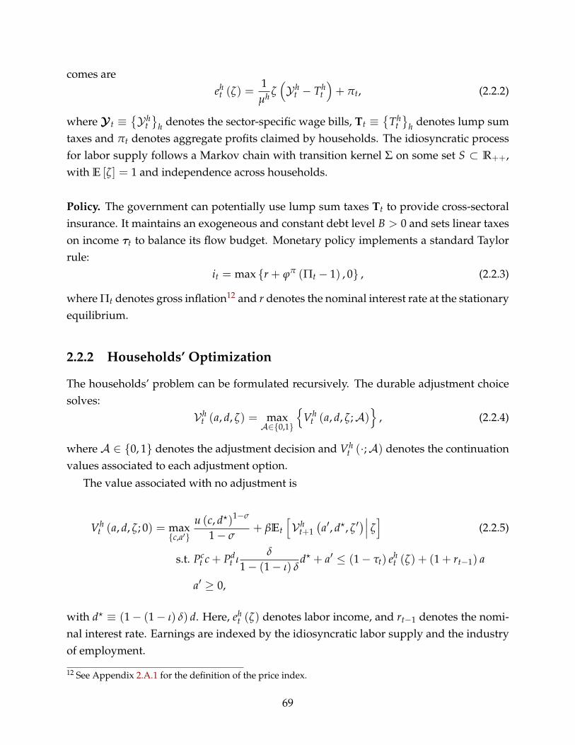
comes areeh

t (ζ) =1

µh ζ(𝒴h

t − Tht

)+ πt, (2.2.2)

where Y t ≡𝒴h

t

h denotes the sector-specific wage bills, Tt ≡

Tht

h denotes lump sumtaxes and πt denotes aggregate profits claimed by households. The idiosyncratic processfor labor supply follows a Markov chain with transition kernel Σ on some set S ⊂ R++,with E [ζ] = 1 and independence across households.

Policy. The government can potentially use lump sum taxes Tt to provide cross-sectoralinsurance. It maintains an exogeneous and constant debt level B > 0 and sets linear taxeson income 𝜏t to balance its flow budget. Monetary policy implements a standard Taylorrule:

it = max r + ϕπ (Πt − 1) , 0 , (2.2.3)

where Πt denotes gross inflation12 and r denotes the nominal interest rate at the stationaryequilibrium.

2.2.2 Households’ Optimization

The households’ problem can be formulated recursively. The durable adjustment choicesolves:

𝒱ht (a, d, ζ) = max

𝒜∈0,1

Vh

t (a, d, ζ;𝒜)

, (2.2.4)

where 𝒜 ∈ 0, 1 denotes the adjustment decision and Vht (·;𝒜) denotes the continuation

values associated to each adjustment option.

The value associated with no adjustment is


c,a′u (c, d?)1−σ

1 − σ+ βEt

[𝒱h

t+1(a′, d?, ζ ′

)∣∣∣ ζ]

(2.2.5)

s.t. Pct c + Pd

t ιδ

1 − (1 − ι) δd? + a′ ≤ (1 − τt) eh

t (ζ) + (1 + rt−1) a

a′ ≥ 0,

with d? ≡ (1 − (1 − ι) δ) d. Here, eht (ζ) denotes labor income, and rt−1 denotes the nomi-

nal interest rate. Earnings are indexed by the idiosyncratic labor supply and the industryof employment.

12 See Appendix 2.A.1 for the definition of the price index.

69

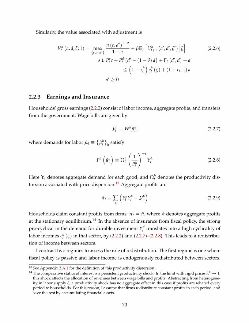
Similarly, the value associated with adjustment is


c,a′,d′u (c, d′)1−σ

1 − σ+ βEt

[𝒱h

t+1(a′, d′, ζ ′

)∣∣∣ ζ]

(2.2.6)

s.t. Pct c + Pd

t(d′ − (1 − δ) d

)+ Γt

(d′, d

)+ a′

≤(

1 − τht

)eh

t (ζ) + (1 + rt−1) a

a′ ≥ 0

2.2.3 Earnings and Insurance

Households’ gross earnings (2.2.2) consist of labor income, aggregate profits, and transfersfrom the government. Wage bills are given by

𝒴ht ≡ Whµh

t , (2.2.7)

where demands for labor t ≡

µht

h satisfy

Fh(

µht

)≡ Ωh

t

(1

Pht

)−ε

Yht (2.2.8)

Here Yt denotes aggregate demand for each good, and Ωht denotes the productivity dis-

torsion associated with price dispersion.13 Aggregate profits are

πt ≡ ∑h

(Ph

t Yht −𝒴h

t

)(2.2.9)

Households claim constant profits from firms: πt = π, where π denotes aggregate profitsat the stationary equilibrium.14 In the absence of insurance from fiscal policy, the strongpro-cyclical in the demand for durable investment Yd

t translates into a high cyclicality oflabor incomes eh

t (ζ) in that sector, by (2.2.2) and (2.2.7)–(2.2.8). This leads to a redistribu-tion of income between sectors.

I contrast two regimes to assess the role of redistribution. The first regime is one wherefiscal policy is passive and labor income is endogenously redistributed between sectors.

13 See Appendix 2.A.1 for the definition of this productivity distorsion.14 The comparative statics of interest is a persistent productivity shock. In the limit with rigid prices λh → 1,

this shock affects the allocation of revenues between wage bills and profits. Abstracting from heterogene-ity in labor supply ζ, a productivity shock has no aggregate effect in this case if profits are rebated everyperiod to households. For this reason, I assume that firms redistribute constant profits in each period, andsave the rest by accumulating financial assets.

70

That is,Tt = 0 (2.2.10)

for each period t.

The second regime (denoted by ?) corresponds to a counterfactual economy wherefiscal policy undoes this redistribution of labor income using lump sum taxes. Specifically,

𝒴dt − µdTd,?

t𝒴 c

t − µcTc,?t

=𝒴d

𝒴 c , (2.2.11)

with budget balance ∑h µhTh,?t ≡ 0, where Y ≡

𝒴h

h denotes wage bills at the sta-tionary equilibrium. This second regime rules out distributional effects and effectivelycorresponds to the case considered in the literature on lumpy durable investment.

2.2.4 Market Clearing

Markets for goods clear:

Yct = ∑

hµh∫ [

cht (a, d, ζ) + Γt

(dh,′

t (a, d, ζ) , d)]

dΛht (2.2.12)

Ydt = ∑

hµh∫ [

dh,′t (a, d, ζ)− (1 − δ) d

]dΛh

t , (2.2.13)

where cht

and dh,′t

denote the solution to (2.2.5)–(2.2.6), with dh,′t

≡ d? when there is no ad-justment. Here, Λt ≡

Λh

t

h denotes the conditional distributions of idiosyncratic stateswithin each sector.

At the stationary equilibrium, wages are flexible and the labor markets clear in the twosectors: 𝜇 = . Then,15

Yht = Fh

(µh)

, (2.2.14)

where µh denotes the exogeneous mass of households located in sector h. However, themarket clearing condition (2.2.14) typically does not hold along the transition path sincewages are fixed. Labor demands are demand-determined:

𝜇 = Zt ∘ t (2.2.15)

15 There is no price dispersion within each sector at the stationary equilibrium, so that denotes bothaggregate and individual labor demands at the steady state.

71

with Zh ≡ 1 at the stationary equilibrium, and 0 ≤ Zht < +∞ along the transition path,

for each sector h and period t. That is, there is rationing of labor incomes in response toaggregate shocks.

Equilibrium. An equilibrium in my economy consists of sequences of policy functionsfor consumption and assets, distributions of idiosyncratic states, and prices, incomes andtaxes such that households and firms optimize, the government balances its budget (andpotentially provides insurance) and monetary policy implements a Taylor rule. I providea formal definition of an equilibrium in Appendix 2.A.2. The economy is initially at itsnon-inflationary stationary equilibrium.

The comparative statics of interest is a one-time, unanticipated, and persistent aggre-gate productivity shock. I assume that this productivity shock is symmetric between thedurable and non-durable sectors, so there is no redistribution of labor incomes in partialequilibrium. Instead, redistribution is induced in general equilibrium by the pro-cyclicalityof durable investment. Financial markets are effectively incomplete with respect to thisaggregate productivity shock.

2.3 Non-Linearity and Redistribution

I introduced a multi-sector model with lumpy investment in the previous section. Durableinvestment plays a dual role in my setting. First, its pro-cyclicality induces a redistributionof labor income between sectors. Second, its lumpiness implies that the average MPC ondurable goods depends on the magnitude of income shocks. In this section, I discuss eachof these roles, and I show that their interaction acts as a non-linear propagation channel.In Section 2.3.1, I discuss the source of aggregate non-linearities in my model. In Section2.3.2, I clarify the role of durable investment as a source of labor income redistribution.I then explore the interaction between these two roles and its aggregate implications inSection 2.3.3. I draw a connection to the existing literatures on redistribution with hetero-geneous agents in Section 2.3.4.

2.3.1 Lumpy Investment and Aggregate Non-Linearity

Durable adjustment is infrequent and discontinuous in my model. I am interested in theaggregate implications of these microeconomic discontinuities. For now, I abstract fromredistribution, so I drop the sector index h.16

16 For notational convenience, I abstract from the masses 𝜇 in (2.2.2).

72

I consider an exogeneous one-time, unanticipated change in aggregate income in pe-riod t = 0:

𝒴0 = (1 + ∆)𝒴

for some ∆ ∈ R, where 𝒴 denotes the aggregate wage bill at the stationary equilibrium.My focus is on the non-linearity of aggregate investment with respect to the size and signof this income shock. I let17

I (∆) ≡∫

∂

∂∆[d′

0(a + ζ∆𝒴 , d, ζ)− (1 − δ) d

]dΛ0 , MPCd

(∆) ≡ dd∆

ℐ (∆) (2.3.1)

denote aggregate durable investment in the first period and the associated average marginalpropensity to spend on durables as functions of the aggregate income shock.

Figure 2.3.1: Response of Aggregate Durable Spending to Income Shocks

Pr A (·) = 1 = θ > 0

(Time-dependent)

A (·) =1 if a ≥ a (·)0 otherwise

(State-dependent)

∆

I (∆)− I (0)

In a companion paper (Zorzi (2020)), I show that MPCd increases with the size of in-come shocks in my model. Put it differently, the response of (aggregate) durable spendingto income shocks I (∆) is convex. I find that this non-linearity is entirely due to adjustmentat the extensive margin. Both the behavior of MPCd and the importance of the extensivemargin are in-line with the empirical evidence (Section 2.4). However, the magnitudespredicted in my calibrated model are substantially lower than their empirical counter-parts.

17 The integration is over the idiosyncratic states (a, d, ζ).

73

Crucially, I find that lumpy durable adjustment together with non-convex adjustmentcosts, i.e. state-dependent adjustment, plays a central role in this form of non-linearity. Incontrast, a model with convex adjustment costs or time-dependent adjustment predicts thatMPCd decreases with the size of income shocks due to a standard precautionary savingsmotive (Carroll and Kimball (1996)). That is, the response of (aggregate) durable spend-ing to income shocks I (∆) is concave. This prediction is counterfactual. Figure 2.3.1 con-trasts these two cases. As discussed in Section 2.3.3, the exact form that this non-linearitytakes plays an essential role in shaping the aggregate effect of income redistribution in myeconomy.

2.3.2 Redistribution in General Equilibrium

I now explore the role of durable investment for the redistribution of labor income in gen-eral equilibrium. Keeping with the rest of the paper, the comparative statics is a one-time,unexpected, and persistent aggregate productivity shock. I assume that this productivityshock is not targeted toward any particular sector, so that redistribution of labor income isentirely induced by endogeneous changes in households’ spending. That is, Ah

t /Ah = At

for each sector h, withlog(

At)= ρA log

(At−1

)+ ψt (2.3.2)

for some persistence ρA ∈ (0, 1) and some innovation ψ0 ∈ R in the first period, withψt ≡ 0 for each consecutive period t ≥ 1.

Following a productivity shock, the pro-cyclicality of durable spending induces a re-distribution of labor income. I impose some restrictions to avoid introducing additionalsources of redistribution. In particular, I assume that technologies and price stickinesssatisfy a certain degree of symmetry across sectors.18

Assumption 4 (Technologies). Technologies are isoelastic and the elasticity is symmetric acrosssectors: Fh

t (l) = Aht lα, for some α ∈ (0, 1) and some vector of productivities At ≡

Ah

t

h.Productivities at the stationary equilibrium A are such that Wc = Wd, i.e. wages are symmetricacross sectors.

Assumption 5 (Price setting). Price stickiness is symmetric across sectors: λh = λ ∈ [0, 1).

18 This symmetry is somewhat restrictive empirically. In particular, the labor share is higher in the durablegood sector, prices of durable goods tend to be more flexible (Bils and Klenow (2004)). These sourcesof heterogeneity and their role over the business cycle have been studied separately (Jaimovich et al.(2019); Pastén et al. (2018)). I choose to abstract from the sources of heterogeneity, to isolate the role ofredistribution induced by cyclical durable investment.

74

Benchmark. To highlight the role of durable investment for the redistribution of labor in-come, I first establish a benchmark where the two goods are non-durable. That is, there isfull depreciation: δ = 1. The relative demand for the two goods is acyclical in this case,by homotheticity of the intratemporal preferences. Under Assumptions 4 and 5, there isno redistribution of labor income and thus no role for insurance from fiscal policy. I for-malize this point in Proposition 2 (Appendix 2.B.1). This benchmark case clarifies that, inmy setting, durability is necessary for income redistribution to take place.19 Furthermore,it confirms that Assumptions 4 and 5 are as neutral as possible: the supply side does notinduce any redistribution per se. I maintain these two assumptions throughout the paper.

Redistribution. Having established this benchmark, I now assume partial depreciation:δ ∈ (0, 1). Durable spending is more cyclical than non-durable spending, which induces aredistribution of labor income across sectors. This redistribution depends on the elasticityof durable investment with respect to income and price changes. In particular, these elas-ticities are governed by: the elasticity of substitution between durables and non-durablesν; the adjustment cost γ; and the maintenance parameter ι.20 In virtually every realisticcalibration, durable investment is more cyclical than non-durable consumption. I assumethat this is the case.

Assumption 6 (Monotonicity). The parameters characterizing the income fluctuations problem(2.2.4)–(2.2.6) are such that relative demand for durable invesment

(dh

t (·)− (1 − δ) d)

/ch (·)and non-durable consumption ch (·) increase with liquid assets.

To understand the pro-cyclicality of relative spending on durable goods, consider arepresentative-agent version of the model presented in Section 2.2.21 In this case,

dt − (1 − δ) dt−1

ct=

1 − ϑ

ϑ

Pct

Pdt − (1−δ)Pd

t+11+rt

ν

︸︷︷︸User cost

− (1 − δ)dt−1

ct︸︷︷︸Stock / flow

at optimum. A productivity shock of the form (2.3.2) affects the relative demand for thedurable investment good through two channels. First, it raises incomes in general equilib-rium. Non-durable consumption and the stock of durable consumption increase propor-tionately. Mechanically, the flow of durable investment is much more volatile. In the first

19 This result is not specific to productivity shocks: the same obtains for monetary policy shocks, deleverag-ing shocks or symmetric tax rebates across sectors.

20 For instance, durable demand is inelastic to income changes as γ → +∞. Similarly, the interest rateelasticity of durable demand is zero as ν → 0.

21 Specifically, there is no idiosyncratic risk (Σ →d 0) and durable adjustment is frictionless (γ = 0).

75

place, this increase in incomes is induced by a fall in the real interest rate, when monetarypolicy is sufficiently responsive (ϕπ > 1). This decrease in the households’ user cost ofdurables tilts spending in favor of durable investment22. This second effect is modulatedby the elasticity of substitution between durables and non-durables (ν).

2.3.3 Aggregate Amplification

In Sections 2.3.1 and 2.3.2, I clarified the dual role of lumpy durable investment in mymodel: its pro-cyclicality induces income redistribution; and micro discontinuities implymacro non-linearities. I now explore the interaction between these two properties, andthe non-linear amplification it generates.

To assess the role of redistribution, I contrast the aggregate response of my economyunder the two regimes (2.2.10)–(2.2.11) for fiscal policy. In the first regime, income redistri-bution takes place between sectors and fiscal policy provides no cross-sectoral insurance.In the second regime, fiscal policy undoes this redistribution and provides full (aggregate)insurance. For tractability, I focus on the general equilibrium response in period t = 0,keeping the sequence of labor incomes, aggregate profits, taxes, interest rates and sector-specific inflation Xt ≡ (Y t, πt, τt, Tt, rt, Πt) fixed for each period t > 1. I also abstract fromchanges in the relative price of durable goods23 by assuming that prices are rigid: λ ≡ 1. Isuppose in the following that MPCd increases with the size of income shocks, consistentlywith the empirical evidence. Again, I include the derivations in Appendix 2.B.2.

Example 4 (Amplification). Consider an expansionary productivity shock: ψ0 < 0.24 La-bor demand increases in both sectors, and so does spending on both goods in partial andgeneral equilibrium, by Assumption 6. However, durable spending is more cyclical sothat 𝒴d

0 /𝒴d > 𝒴 c0/𝒴 c, i.e. labor income is redistributed in favor of the durable sector.

Now, suppose that fiscal policy undoes this redistribution by providing aggregate in-surance, using lump sum taxes (2.2.11),

Td0 = −µc

µd Tc0 > 0

These transfers reduce the dispersion in the distribution of labor incomes. Assume that

22 This second channel is particularly powerful in typical models of investment. Existing estimate suggestthat this effect is overstated (Hall (1977); Shapiro (1986); McKay and Wieland (2019)).

23 The relative price of durable goods is mostly acyclical in the data (Pistaferri (2016); Cantelmo and Melina(2018); McKay and Wieland (2019)).

24 Note that a positive productivity shock (ψ0 > 0) is contractionary with rigid prices, since households claimconstant profits from firms in my setting. The evidence on the effect of technology improvements on labordemand is mixed. References include Basu et al. (2006) and Alexopoulos (2011), among others.

76

aggregate durable spending by households employed in each sector

Yd,h0 ≡

∫ [dh,′

0 (a, d, ζ)− (1 − δ) d]

dΛh0

is convex in (sectoral) incomes,25 for each sector h. By Jensen’s inequality, a lower disper-sion due to fiscal policy depresses aggregate durable investment Yd

0 ≡ ∑h µhYd,h0 . Put it

differently, endogeneous income redistribution between sectors amplifies the effect of anexpansionary productivity shocks, compared to a benchmark with full aggregate insur-ance. Symmetrically, income redistribution dampens the effect of contractionary shocks.

Figure 2.3.2: Impulse Response of Aggregate Durable Spending

State-Dependent Adjustment

ψ0

Y d0

Time-Dependent Adjustment

ψ0

Y d0

Insurance No insurance

Lumpy and state-dependent adjustment is key to this non-linear amplification. Fig-ure 2.3.2 contrasts the predictions of models with state- and time-dependent adjustment.As illustrated in Figure 2.3.1, the response of (aggregate) durable spending is concave in(sectoral) incomes with time-dependent adjustment. Therefore, endogeneous income re-distribution depresses aggregate demand. As a result, cyclical income inequality dampensthe response of durable spending to expansionary shocks, and amplifies the response tocontractionary shocks. A realistic micro-foundation of the durable adjustment hazard isthus crucial to understand the effect of income redistribution on aggregate durable spend-ing.

25 Incomes are implicit to the time index.

77

2.3.4 Sufficient Statistics

The effect of income redistribution in my model can be understood through a sufficientstatistics approach. To simplify the exposition, I suppose that the average income is sym-metric across sectors at the stationary equilibrium. Furthermore, I focus on the first period(t = 0), by asumming that fiscal policy provides full (aggregate) insurance across sectorsin the following periods (t ≥ 1).26

Aggregate durable spending (2.2.13) can be decomoposed as follows:27

Yd0 = ∑

hµh∫

ℐ0 (a, d, e0 (ζ)) dΛh

︸︷︷︸(Aggregate) insurance

+∑h

µh∫ eh

0−e0

0MPCd

0 (z) dz︸︷︷︸Redistribution

(2.3.3)

Here, e0 (ζ) ≡ ∑h µheh0 (ζ) denotes the average income across sectors conditional a level of

productivity, eh0 ≡

∫eh

0 (ζ) dΛh denotes average income within a sector, e0 ≡∫

e0 (ζ) dΛdenotes the average income across sectors and ℐ0 denotes investment at the householdlevel as a function of current income.

The first term in (2.3.3) corresponds to aggregate durable spending when fiscal policyprovides full (aggregate) insurance, i.e. (2.2.11) holds. In turn, the second term capturesthe effect of income redistribution when fiscal policy is passive, i.e. (2.2.10) holds. Thisterm depends on two endogeneous objects: the extent of income redistribution betweensectors eh

0 − e0; and the response of the average marginal propensity to spend on durablesMPCd

0 to (sectoral) income changes. The behavior of these two objects was discussed inSections 2.3.1 and 2.3.2. Incomes are more elastic to productivity shocks in the durablesector, and the average MPC on durables increases with the size of income changes. I nowput these pieces together to understand how endogeneous income redistribution affectsthe response to aggregate shocks.

To assess the role of income redistribution, I start by comparing the first order re-sponses of durable spending to a productivity shock under the two regimes of interest:28

ddψ

(Yd

0 (0)− Yd,?0 (0)

)= Cov

(d

dψ

(eh

0 (0)− e0 (0))

, MPCd0 (0)

)where the covariance is over sectors h. My model is set up so that there is no ex-ante

26 That is, incomes are symmetric across sectors for t ≥ 1 conditional on a level of productivity (ζ).27 With full (aggregate) insurance for periods t ≥ 1, households’ current income (e) is a sufficient statistics

for their productivity and sector of employment.28 I make the dependence of durable spending and incomes on the innovation in productivity (ψ) in (2.3.2)

explicit. Again, the full (aggregate) insurance regime is denoted by ?.

78

heterogeneity in average MPCs on durables between sectors: MPCd,c0 = MPCd,d

0 ≡ MPCd0

at the stationary equilibrium.29,30 In other words, the “earnings heterogeneity channel”studied by Auclert (2019), Werning (2015) and Patterson (2019) has no aggregate effects inmy model for first order deviations from the stationary equilibrium. As a consequence,the response of durable spending does not depend on the degree of insurance from fiscalpolicy for infinitesimal aggregate shocks.

I now consider a discrete, expansionary shock (ψ < 0).31 In this case, the second termin (2.3.3) is positive when fiscal policy is passive:

ed0 − e0 = −µc

µd (ec0 − e0) < 0 =⇒

∫ ed0−e?0

0MPCd

0 (z) > −µc

µd

∫ ec0−e?0

0MPCd

0 (z)

since MPCd0 is (strictly) increasing. Those who benefit from income redistribution during

an expansion are willing to spend more on durables at the margin. Therefore, income re-distribution amplifies the response of aggregate durable spending to expansionary shocks.The case of contractionary shock (ψ > 0) is symmetric. Those who suffer more from in-come redistribution during a contraction cut back less on durable spending. Therefore,income redistribution dampens the response of aggregate durable spending to contrac-tionary shocks. Summing up:

Yd0 (ψ)− Yd,?

0 (ψ)

> 0 if ψ < 0

= if ψ = 0

< 0 otherwise

Taken together, these observations explain why the response without insurance definesthe upper envelope of the response with insurance in the left panel of Figure 2.3.2.

2.3.5 Timing and Redistribution

The analysis above assumed that income shocks were fully transitory. Households arenon-Ricardian in my model due to borrowing constraints, so the timing of income shocks

29 The distribution of financial and durable holdings is symmetric across sectors at the stationary equilib-rium, by Assumption 4.

30 I focus on one-time, unanticipated shocks. If households employed in the durable sector anticipatedaggregate risk, they could in theory accumulate higher precautionary savings. There is only limited em-pirical support for this prediction (Skinner (1988)), which can partly be attributed to heterogeneity inrisk-aversion across sectors (Schulhofer-Wohl (2011)). Patterson (2019) finds that heterogeneity in MPCsacross sectors plays a relatively minor role in the general equilibrium amplification of aggregate shocks.

31 Again, a positive productivity shock (ψ0 > 0) is contractionary with rigid prices.

79

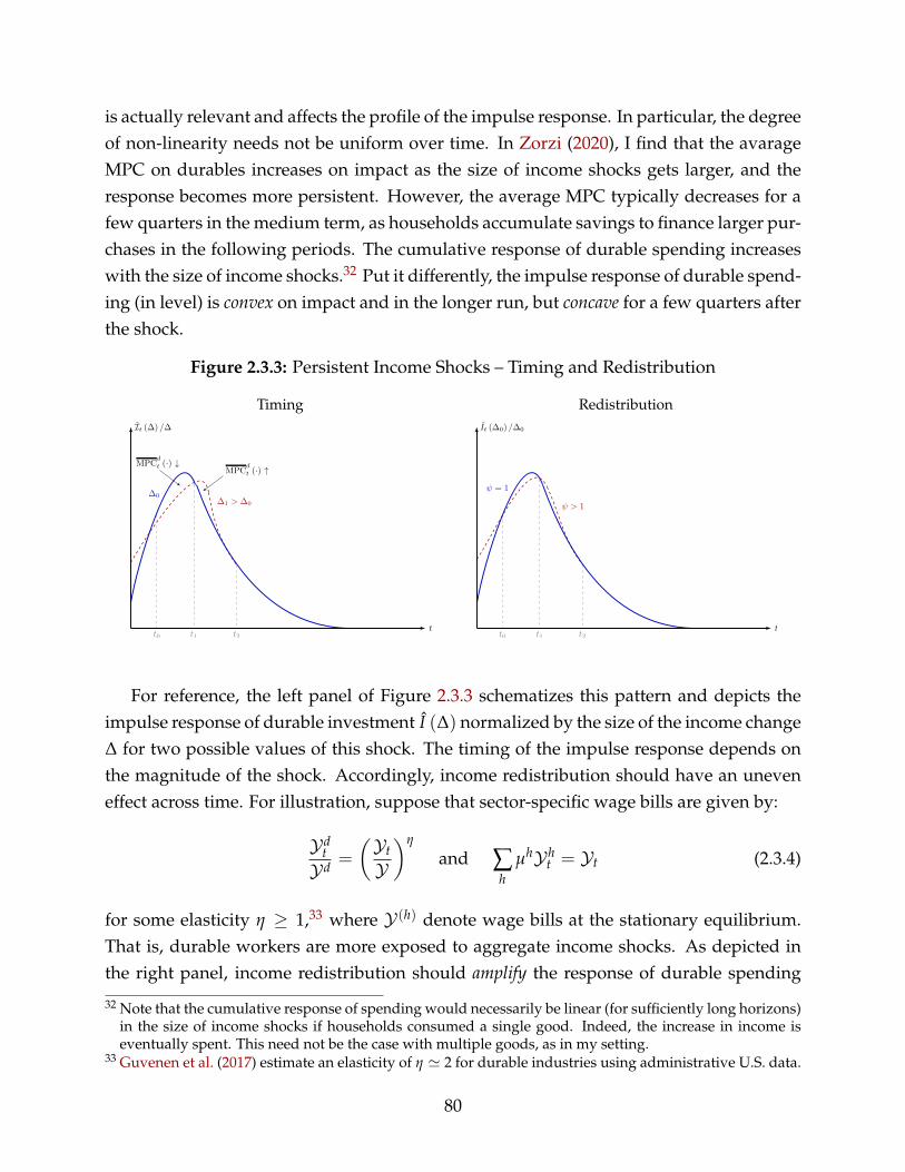
is actually relevant and affects the profile of the impulse response. In particular, the degreeof non-linearity needs not be uniform over time. In Zorzi (2020), I find that the avarageMPC on durables increases on impact as the size of income shocks gets larger, and theresponse becomes more persistent. However, the average MPC typically decreases for afew quarters in the medium term, as households accumulate savings to finance larger pur-chases in the following periods. The cumulative response of durable spending increaseswith the size of income shocks.32 Put it differently, the impulse response of durable spend-ing (in level) is convex on impact and in the longer run, but concave for a few quarters afterthe shock.

Figure 2.3.3: Persistent Income Shocks – Timing and Redistribution

Timing

t0 t1 t2

∆0∆1 > ∆0

MPCd

t (·) ↑MPC

d

t (·) ↓

t

It (∆) /∆

Redistribution

t0 t1 t2

ψ > 1

ψ = 1

t

It (∆0) /∆0

For reference, the left panel of Figure 2.3.3 schematizes this pattern and depicts theimpulse response of durable investment I (∆) normalized by the size of the income change∆ for two possible values of this shock. The timing of the impulse response depends onthe magnitude of the shock. Accordingly, income redistribution should have an uneveneffect across time. For illustration, suppose that sector-specific wage bills are given by:

𝒴dt

𝒴d =

(𝒴t

𝒴

)η

and ∑h

µh𝒴ht = 𝒴t (2.3.4)

for some elasticity η ≥ 1,33 where 𝒴 (h) denote wage bills at the stationary equilibrium.That is, durable workers are more exposed to aggregate income shocks. As depicted inthe right panel, income redistribution should amplify the response of durable spending

32 Note that the cumulative response of spending would necessarily be linear (for sufficiently long horizons)in the size of income shocks if households consumed a single good. Indeed, the increase in income iseventually spent. This need not be the case with multiple goods, as in my setting.

33 Guvenen et al. (2017) estimate an elasticity of η ≃ 2 for durable industries using administrative U.S. data.

80

on impact and increase its persistence, since the response of durable spending is convexin the size of income shocks over the corresponding range. On the contrary, income re-distribution should dampen the response of durable spending for a few quarters after theoccurrence of the shock. The general equilibrium responses I obtain in Section 2.6 confirmthese predictions.

2.4 Supporting Evidence

In this section, I briefly review supporting evidence on the interaction between the cycli-cality of durable spending and income redistribution.

2.4.1 Redistribution

Purchases of durable goods and residential investment are strongly pro-cyclical in the data(Kydland and Prescott (1982); Baxter (1996)). Hall (2005) and Bils et al. (2013) documenta substantial pass-through to durable employment during booms and busts. Using ad-ministrative U.S. data, Guvenen et al. (2017) confirm that expansions and recessions havedistributional consequences between workers employed in durable and non-durable sec-tors.34

I illustrate the importance of this sectoral income redistribution in two contexts: theGreat Recession; and in response to well-identified, exogeneous shocks. To account forcross-sectoral labor mobility and movements in and out of the labor force, I use longitudi-nal data from the Panel Study of Income Dynamics (PSID).35 The PSID is a representativepanel survey of U.S. households conducted annually during 1968-1997, and bi-annuallysince then. The sample consists of male household’s heads aged 24-65. To eliminate out-liers, I exclude households with labor income lower than 5% of the annual average, andhigher than the 95th percentile. I use (real) gross labor incomes as an empirical counter-part to labor earnings in my model.36 I describe the data, the sample selection, and thespecifications in Appendix 2.C.

The left panel of Figure 2.4.1 plots the time series of real spending during the Great

34 They estimate a contemporaneous elasticity of individual income with respect to GDP of roughly 2 fordurable industries.

35 Other datasets commonly used for the study of income dynamics – such as the Current Population Survey(CPS), the Survey of Income and Program Participation (SIPP), or the National Longitudinal Survey ofYouth (NLSY) – either have a shorter panel dimension, or their sample is not as representative of the U.S.population as the PSID’s.

36 I also report the responses for family income in Appendix 2.C.3 to account for unemployment insuranceand intra-household risk-sharing. The conclusions are very similar in this case.

81

Recession for the two categories of interest: durables and residential investment; and non-durables and services. Durable spending fell by roughly 25% over this period, comparedto 5% for non-durable spending. The right panel plots the time series of mean labor in-come for households employed in the corresponding sectors in 2008.37 The recession ledto a substantial redistribution of labor income between sectors. The pass-through was in-complete, however. Labor incomes in durable sectors decreased by 13% over two years,compared to a 4% decline in non-durable sectors.

Figure 2.4.1: Great Recession

Spending Gross Labor Incomes (PSID)

Durables and residential investment Non-durables and services

For robustness, I estimate the sector-specific response of labor incomes to well identi-fied, exogeneous shocks. The leading example in my paper is an unanticipated produc-tivity shocks. Fluctuations in measured productivity are potentially endogeneous, how-ever.38 To address this concern, I focus instead on narratively-identified, exogeneous pol-icy shocks. I use the series of exogeneous tax changes constructed by Romer and Romer(2010),39 which are sufficiently persistent to be aggregated at the low-frequency of thePSID data.

The left panel of Figure 2.4.2 plots the response of spending on durables and non-durables following a one-standard deviation contractionary Romer and Romer (2010) tax

37 Specifically, I allocate households to either the durable or non-durable sectors based on their industry ofemployment in 2008 (i.e. 2009 PSID wave). Fixing this cross-section, I compute mean labor income foreach year.

38 See Chari et al. (2007) and Buera and Moll (2015), among others. Productivity shocks identified via Struc-tural Vector Auto-Regression (SVAR) might not be exogeneous either (Ramey (2011)).

39 I prefer tax changes to government spending shocks (Ramey (2011)). Those are typically targeted towarda particular sector, which mechanically induces redistribution.

82

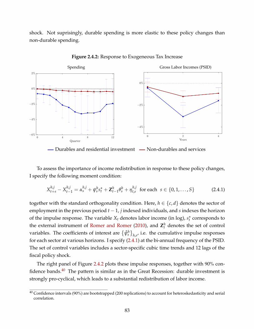
shock. Not suprisingly, durable spending is more elastic to these policy changes thannon-durable spending.

Figure 2.4.2: Response to Exogeneous Tax Increase

Spending Gross Labor Incomes (PSID)


To assess the importance of income redistribution in response to these policy changes,I specify the following moment condition:

Xh,jt+s − Xh,j

t−1 = αh,js + ψh

s s?t + Zht−1θh

s + ηh,jt,s for each s ∈ 0, 1, . . . , S (2.4.1)

together with the standard orthogonality condition. Here, h ∈ c, d denotes the sector ofemployment in the previous period t− 1, j indexed individuals, and s indexes the horizonof the impulse response. The variable Xt denotes labor income (in log), s?t corresponds tothe external instrument of Romer and Romer (2010), and Zh

t denotes the set of controlvariables. The coefficients of interest are

ψh

s

h,s, i.e. the cumulative impulse responsesfor each sector at various horizons. I specify (2.4.1) at the bi-annual frequency of the PSID.The set of control variables includes a sector-specific cubic time trends and 12 lags of thefiscal policy shock.

The right panel of Figure 2.4.2 plots these impulse responses, together with 90% con-fidence bands.40 The pattern is similar as in the Great Recession: durable investment isstrongly pro-cyclical, which leads to a substantial redistribution of labor income.

40 Confidence intervals (90%) are bootstrapped (200 replications) to account for heteroskedasticity and serialcorrelation.

83

2.4.2 Increasing MPCs

In my model, the average MPC out of an income shock increases with the size of thisshock (Section 2.3.1). This property ensures that cyclical income inequality has aggregateeffects.

The literature estimates a wide range of MPCs on durables. In particular, Johnson etal. (2006) find negligible spending multipliers on durable goods in the context of the 2001stimulus payment. On the contrary, Souleles (1999) estimates that the response of spend-ing to springtime tax refunds is almost entirely driven by durable expenditure (and pur-chases of vehicles in particular), while Parker et al. (2013) document sizeable multipliersfollowing the larger stimulus payment in 2008. Parker et al. (2013) attribute the differencein MPCs across these episodes to the size of the corresponding transfers. These findingsare in-line with the survey evidence of Fuster et al. (2018) and Christelis et al. (2019), whodocument that the average MPC on durables increases with the size of (hypothetical) taxrebates.

In Zorzi (2020), I compare the predictions of my model with the existing empirical ev-idence. I find that the model generates the correct form of non-linearity. However, themagnitudes are substantially lower than those observed in the data. This small degree ofnon-linearity artificially dampens the general equilibrium effect of income redistributionin my structural model. As a consequence, the effect that I obtain in my general equilib-rium exercise (Section 2.6) should be thought of as very conservative lower bounds on theactual effect.

2.5 Calibration

The remainder of the paper quantifies the mechanisms documented in Section 2.3. I firstparametrize the model using a mix of external and internal calibration. Following Bergerand Vavra (2015), I adopt a broad definition of durable goods that includes residentialinvestment and consumer durables.

I calibrate five parameters internally: the discount factor (β), the preference parameterfor non-durable goods (ϑ), the durable adjustment costs (γ), the exogeneous supply ofliquidity (B), and the relative productivity in the durable sector

(Ad). I calibrate the

remaining parameters externally, using standard values in the literature. I first review theexternal calibration, before discussing the targeted moments and the fitted parameters.Table 2.5.2 describes the parametrization. Data sources are listed in Appendix 2.C.1.

84

2.5.1 External Calibration

I set the inverse elasticity of intertemporal substitution to σ = 4. This value, while largecompared to typical calibrations, is commonly used in models with durable goods (Guer-rieri and Lorenzoni (2017); McKay and Wieland (2019)), which predict a high elasticity ofdurable investment to interest rate changes. I choose a unitary elasticity of substitutionbetween durables and non-durables ν → 1, following Berger and Vavra (2015).41 I choosea maintenance parameter of ι = 0.5, which lies between the estimates of Berger and Vavra(2015) (ι = 0.8) and McKay and Wieland (2019) (ι = 0.35).

The stock of durable goods depreciates at roughly 2% (δ = 0.018). The income process(in log) follows an AR(1) process with persistence ρ = 0.975 and standard deviation ofinnovations σ = 0.1 to match the evidence of Floden and Lindé (2001). I set the massof households in the durable sector to µd = 0.187, based on data from the Current Em-ployment Statistics (see Appendix 2.C.1). Based on Assumptions 4 and 5, I assume acertain degree of symmetry between sectors. Technologies are isoelastic and the elastic-ity is symmetric across sectors. I normalize productivity to 1 in the non-durable sector.Labor receives roughly 2/3 of revenues at the stationary equilibrium (α = 0.3). Simi-larly, price stickiness is symmetric across sectors. With imperfectly sticky prices

(λh < 1

),

the cyclicality of durable spending induces substantial changes in the relative price ofdurable goods. This prediction is not verified in the data, however.42 Furthermore, mod-els of lumpy investment typically predict an excessively high elasticity to changes in usercost.43 For this reason, I assume that prices are fixed λh = 1 for my general equilibriumexercise (Section 2.6). Note that the elasticity of substitution across varieties (ε = 10) andthe coefficient in the monetary policy rule (ϕ = 1.25) are irrelevant in this case.

2.5.2 Internal Calibration

The remaining parameters(

β, ϑ, γ, B, Ad), together with the interest rate (r) and the priceof the durable good

(Pd) at the stationary equilibrium, are the implicit solution to seven

restrictions: two equilibrium conditions, and five empirical moments. The moments I tar-get, their values and the sources I use are listed in Table 2.5.1.44 Appendix 2.A.4 describesthe calibration strategy in more details.

41 The literature has typically used a unitary elasticity, based on the estimates of Ogaki and Reinhart (1998)and Piazzesi and Schneider (2007). However, values below unity are sometimes used to dampen theinterest rate elasticity of durable demand (Barsky et al. (2016); McKay and Wieland (2019)).

42 See Pistaferri (2016), Cantelmo and Melina (2018) and McKay and Wieland (2019), among others.43 House (2014) and Winberry (2019) make this point in the context of capital investment, and McKay and

Wieland (2019) in the context of durable spending.44 In Table 2.5.1, “relative” refers to the ratio of the value for durable to that for non-durable.

85

I choose the discount factor β to target a real interest rate at the stationary equilibriumof 2.5%, which corresponds to the average value since 1970. I set the preference parameterfor non-durable goods ϑ to obtain a ratio of investment to consumption of roughly 18%.I adjust the durable adjustment parameter γ to target an annual frequency of adjustmentof 12%, as in Berger and Vavra (2015). I obtain γ = 0.025, which corresponds to an ad-justment cost of 3.3% when expressed in terms of the numéraire.45 The exogeneous supplyof liquidity (B) targets a ratio of liquidity to annual GDP of 1.4, following McKay et al.(2016).46 Finally, I choose the relative productivity in the durable goods sector Ad to targetsymmetric wages across sectors at the stationary equilibrium.

Table 2.5.1: Targeted Moments

Target Value Source

Real interest rate (A) 0.025 FRED and NIPA

Ratio of investment to consumption 0.18 NIPA

Frequency of durable adjustment (A) 0.10 Berger and Vavra (2015)

Liquidity supply to GDP (A) 1.4 McKay et al. (2016)

Relative wages 1 Normalization

2.6 General Equilibrium

In the previous sections, I discussed the source of non-linearities in my model and how itinteracts with income redistribution in general equilibrium. I now explore the quantitativeimportance of this mechanism.

I simulate the response of my general equilibrium model to aggregate disturbances.Following Berger and Vavra (2015), I focus on productivity shocks. Income redistributionbetween sectors takes place endogeneously in my model, as durable investment respondsmore strongly than non-durable consumption.

The left panel of Figure 2.6.1 plots the general equilibrium responses of durable invest-ment and non-durable consumption to an persistent, expansionary productivity shock of5% with a half-life of 6 quarters. As expected, the impulse response of durable spending is

45 This figure is slightly lower than the 5% typically used in the literature (Díaz and Luengo-Prado (2010);Berger and Vavra (2015)). However, the relative price of durables is larger than 1 in my model, whichreduces the frequency of adjustment for any fixed cost.

46 Liquidity includes: deposits, government-issued securities, corporate bonds and equitities and mutualfund shares.

86

Table 2.5.2: Calibration

Parameter Description Calibration Source / Target

Preferencesβ Discount factor 0.985 Internal calibrationν Elasticity of substitution 1 See textϑ Non-durable parameter 0.731 Internal calibrationσ EIS (inverse) 4 See textε Elasticity of substitution (inverse) 10 Kaplan et al. (2018)

Durable goodsδ Depreciation rate 0.018 Berger and Vavra (2015)γ Adjustment cost 0.025 Internal calibrationι Maintenance parameter 0.5 See text

Income processρ Persistence 0.967 Floden and Lindé (2001)σ Standard deviation 0.13 Floden and Lindé (2001)

LiquidityB Ratio of bond supply to GDP 1.490 Internal calibration

Labor supplyµd Mass of households (durable) 0.187 CES

ProductionAd Relative productivity (durable) 0.490 Internal calibrationα Decreasing returns 0.3 Berger and Vavra (2015)

Prices and policyλ Calvo parameter 1 See textϕ Taylor rule coefficient (inflation) 1.25 Kaplan et al. (2018)

87

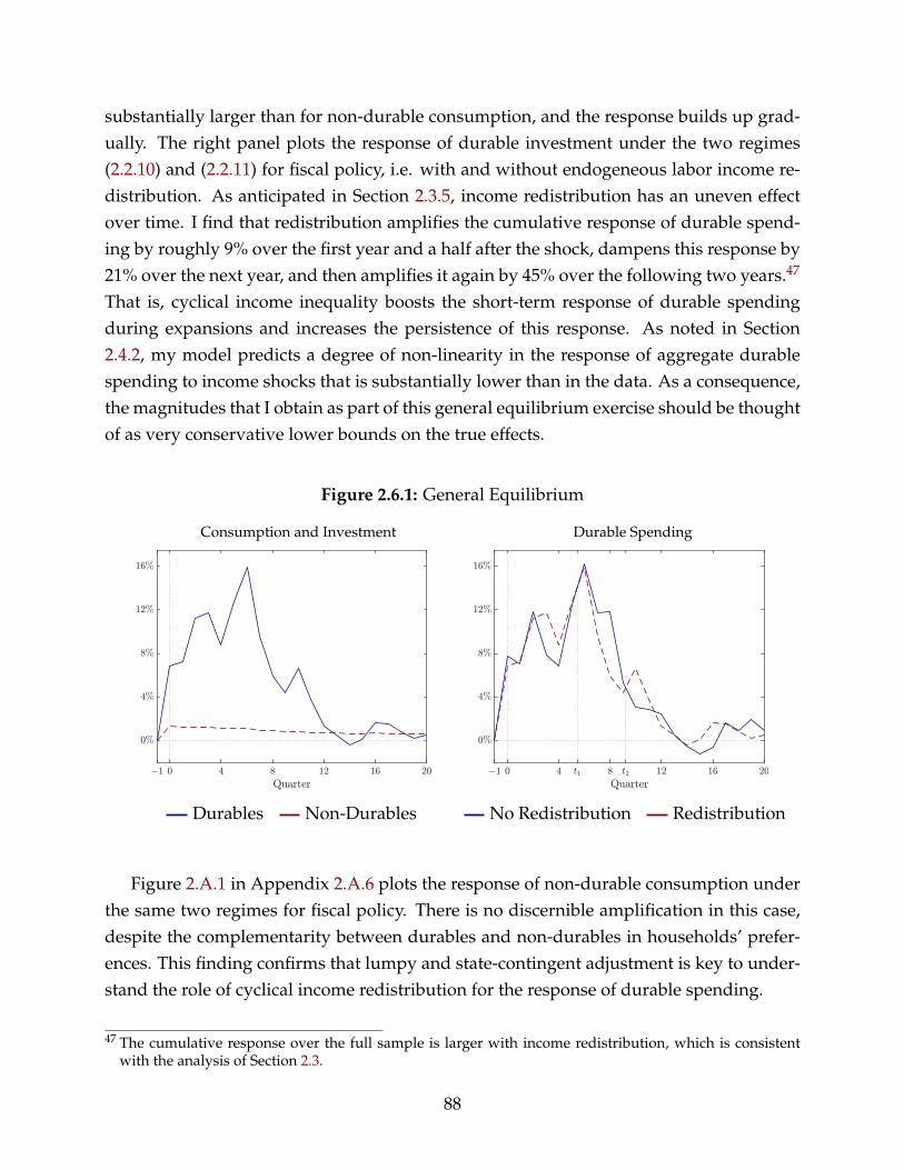
substantially larger than for non-durable consumption, and the response builds up grad-ually. The right panel plots the response of durable investment under the two regimes(2.2.10) and (2.2.11) for fiscal policy, i.e. with and without endogeneous labor income re-distribution. As anticipated in Section 2.3.5, income redistribution has an uneven effectover time. I find that redistribution amplifies the cumulative response of durable spend-ing by roughly 9% over the first year and a half after the shock, dampens this response by21% over the next year, and then amplifies it again by 45% over the following two years.47

That is, cyclical income inequality boosts the short-term response of durable spendingduring expansions and increases the persistence of this response. As noted in Section2.4.2, my model predicts a degree of non-linearity in the response of aggregate durablespending to income shocks that is substantially lower than in the data. As a consequence,the magnitudes that I obtain as part of this general equilibrium exercise should be thoughtof as very conservative lower bounds on the true effects.

Figure 2.6.1: General Equilibrium

Consumption and Investment Durable Spending

Durables Non-Durables No Redistribution Redistribution

Figure 2.A.1 in Appendix 2.A.6 plots the response of non-durable consumption underthe same two regimes for fiscal policy. There is no discernible amplification in this case,despite the complementarity between durables and non-durables in households’ prefer-ences. This finding confirms that lumpy and state-contingent adjustment is key to under-stand the role of cyclical income redistribution for the response of durable spending.

47 The cumulative response over the full sample is larger with income redistribution, which is consistentwith the analysis of Section 2.3.

88

2.7 Conclusion

In this paper, I study the implications of cyclical income inequality for the dynamics ofaggregate durable spending. I explore this question using a multi-sector heterogeneousagent (HANK) model with lumpy durable investment. Durable demand plays a dual rolein my setting. First, its pro-cyclicality induces a redistribution of labor income betweendurable and non-durable sectors. Second, lumpy durable adjustment at the micro levelproduces non-linearities at the macro level: the average MPC on durable goods increaseswith income changes. As a result, income redistribution has aggregate effects. It amplifiesthe response to expansionary shocks, and dampen that to contractionary shocks.

I first clarify these mechanisms analytically. I then simulate numerically the responseof durable spending to productivity shocks in general equilibrium. I find that cyclicalincome inequality affects both the short-term response of durable spending and the per-sistence of this response.

89



In this Appendix, I present the full model and describe the approach used to simulate andcalibrate the model. Section 2.A.1 describes the full model. Section 2.A.2 provides a formaldefinition of an equilibrium. Section 2.A.3 provides the algorithm used to solve for thestationary equilibrium and the transition dynamics. I discuss the calibration strategy inSection 2.A.4. Finally, Section 2.A.5 provides details about the numerical implementation.

2.A.1 Environment

For concision, Section 2.2 provided a partial description of the environment. For reference,I now present the full model.

Timing. Periods are indexed by t ∈ 0, 1, . . .. There is no aggregate risk. I focus onone-time, unanticipated but persistent shocks. Each period effectively consists of two sub-periods, indexed by t.0 (−) and t.1 (+). Households make their adjustment decisions att.0, and their consumption, saving and investment decisions at t.1. In period t.0, house-holds are indexed by their financial asset holdings (a), their holdings of durable goods(d), their idiosyncratic labor supply shock (ζ) and the sector they are employed in (h). Inperiod t.1, households are in addition indexed by their adjustment choice (𝒜) during theprevious sub-period.48 The conditional distributions of idiosyncratic states within eachsector, at the begining of each subperiod, are denoted by Λ−

t−1 and Λ+t . All agents have

perfect foresight, and all (aggregate) information is revealed at the begining of the firstsub-period at t = 0.

Households. The households’ value function in period t.0 satisfies:

48 This additional state variable is for notational convenience. Financial assets are a sufficient statistics forthis adjustment.

91

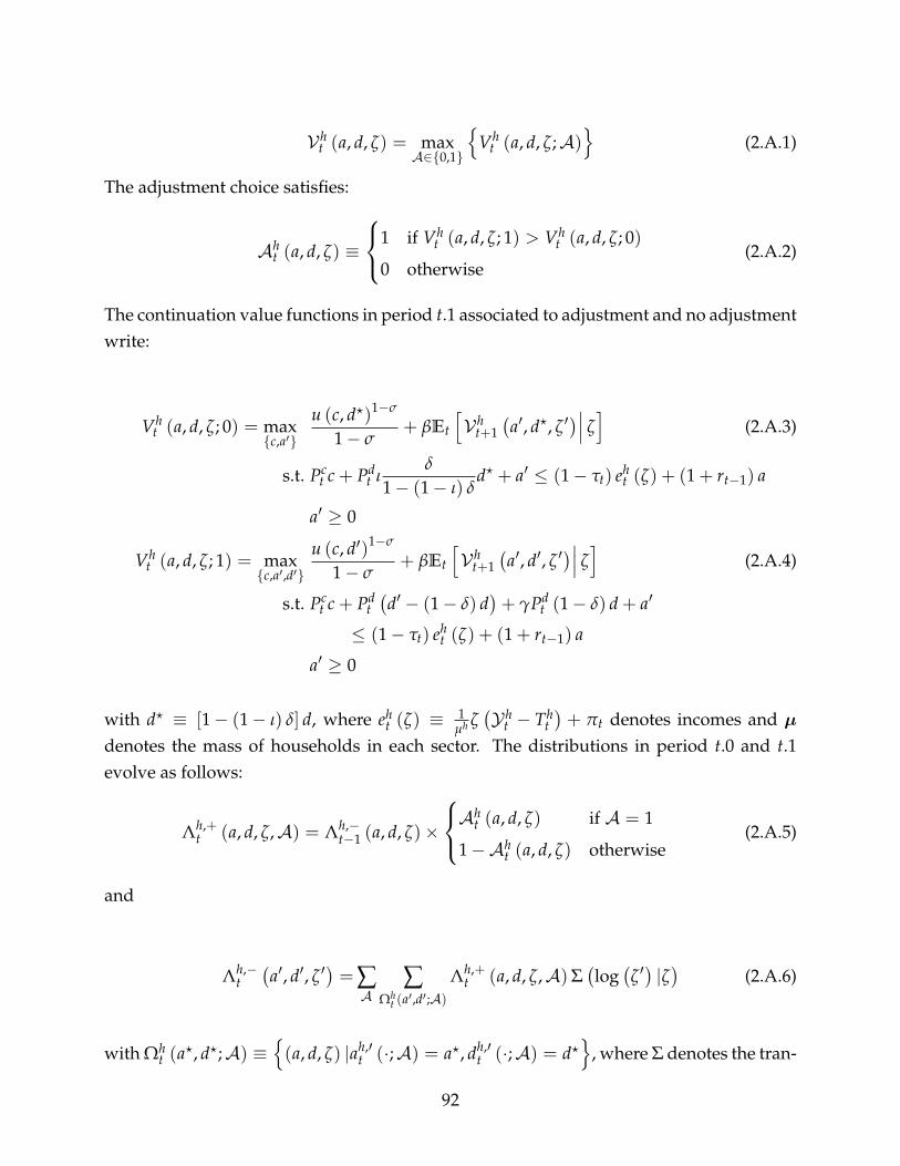
𝒱ht (a, d, ζ) = max

𝒜∈0,1

Vh

t (a, d, ζ;𝒜)

(2.A.1)

The adjustment choice satisfies:

𝒜ht (a, d, ζ) ≡

1 if Vht (a, d, ζ; 1) > Vh

t (a, d, ζ; 0)

0 otherwise(2.A.2)

The continuation value functions in period t.1 associated to adjustment and no adjustmentwrite:


c,a′u (c, d?)1−σ

1 − σ+ βEt

[𝒱h

t+1(a′, d?, ζ ′

)∣∣∣ ζ]

(2.A.3)

s.t. Pct c + Pd

t ιδ

1 − (1 − ι) δd? + a′ ≤ (1 − τt) eh

t (ζ) + (1 + rt−1) a

a′ ≥ 0


c,a′,d′u (c, d′)1−σ

1 − σ+ βEt

[𝒱h

t+1(a′, d′, ζ ′

)∣∣∣ ζ]

(2.A.4)

s.t. Pct c + Pd

t(d′ − (1 − δ) d

)+ γPd

t (1 − δ) d + a′

≤ (1 − τt) eht (ζ) + (1 + rt−1) a

a′ ≥ 0

with d? ≡ [1 − (1 − ι) δ] d, where eht (ζ) ≡ 1

µh ζ(𝒴h

t − Tht)+ πt denotes incomes and 𝜇

denotes the mass of households in each sector. The distributions in period t.0 and t.1evolve as follows:

Λh,+t (a, d, ζ,𝒜) = Λh,−

t−1 (a, d, ζ)×

𝒜ht (a, d, ζ) if 𝒜 = 1

1 −𝒜ht (a, d, ζ) otherwise

(2.A.5)

and

Λh,−t(a′, d′, ζ ′

)=∑

𝒜∑

Ωht (a′,d′;𝒜)

Λh,+t (a, d, ζ,𝒜)Σ

(log(ζ ′)|ζ)

(2.A.6)

with Ωht (a?, d?;𝒜) ≡

(a, d, ζ) |ah,′

t (·;𝒜) = a?, dh,′t (·;𝒜) = d?

, where Σ denotes the tran-

92

sition kernel characterizing the income process and ah,′t

and dh,′t

denote the solution to(2.A.1)–(2.A.4), with dh,′

t≡ d? when no adjustment. I define ch

tsimilarly.

Firms. Prices are sticky along the transition path:

(Ph

t

)1−ε= λh

(Ph

t−1

)1−ε+(

1 − λh) (

P?,ht

)1−ε(2.A.7)

with initial condition Ph−1 ≡ Ph, i.e. prices at the stationary equilibrium. Reset prices P?t

satisfy:

P?,ht =

[1

1 − α

ε

ε − 1Gh

t

Hht

] 1−α(1−α)(1−ε)+ε

(2.A.8)

in each sector h, with

Ght =Wh

( 1Ph

t

)−εYh

tAh

11−α

+ λh 11 + rt

Ght+1 (2.A.9)

Hht =

(1

Pht

)−ε

Yht + λh 1

1 + rtHh

t+1 (2.A.10)

for each t ∈ 0, 1, . . . , T − 1, and

GhT =

1 + r1 + r − λh Wh

[(1

Ph

)−ε Yh

Ah

] 11−α

HhT =

1 + r1 + r − λh

(1Ph

)−ε

Yh

for each sector h, where W denotes nominal nominal wages at the stationary equilibrium,and (Y, P, r) denotes aggregate demands for each good, prices and the nominal interestrate at the steady state.

Policy. Depending on the regime of interest (insurance, or not), lump sum taxes satisfy:

Tt = 0 or𝒴d

t − µdTdt

𝒴 ct − µcTc

t=

𝒴d

𝒴 c (2.A.11)

with ∑h µhTht ≡ 0, where Y denotes wages bills at the stationary equilibrium The govern-

93

ment’s flow budget constraint is

τt ∑h

µh∫

eht (ζ) dΛh

t = −rt−1B (2.A.12)

Monetary policy implements a Taylor rule:

it = max r + ϕπ (Πt − 1) , 0 (2.A.13)

Here, Πt − 1 ≡ ∆ log(

Pt)

denotes the inflation rate, where

Pt ≡[

ϑ (Pct )

1−ν + (1 − ϑ)(

Pdt

)1−ν] 1

1−ν

(2.A.14)

denotes the CES ideal price index.

Market clearing. Markets for goods clear:

Yct = ∑

hµh∫ [

cht (a, d, ζ) + Γt

(dh,′

t (a, d, ζ) , d)]

dΛh,+t (2.A.15)

Ydt = ∑

hµh∫ [

dh,′t (a, d, ζ)− (1 − δ) d

]dΛh,+

t (2.A.16)

The TFP component associated to price dispersion is

(Ωh

t

) 11−αh ≡ λh

(Ωh

t−1

) 11−αh

+(

1 − λh) (

Ph,?t

)− ε

1−αh (2.A.17)

with Ωh−1 ≡

(Ph)−ε

. Demands for labor satisfy

µht ≡ Ωh

t

1Ah

(1

Pht

)−ε

Yht

11−α

(2.A.18)

with Ωht ≡

(Ωh

t) 1

1−αh . Wage bills and aggregate profits write

𝒴ht = Whµh

t (2.A.19)

πt = ∑h

(Ph

t Yht −𝒴h

t

), (2.A.20)

94

Households claim constant profits from firms: πt = π, where π denotes aggregate profitsat the stationary equilibrium. In turn,

𝜇 = Zt ∘ t (2.A.21)

with Zh ≡ 1 at the stationary equilibrium, and 0 ≤ Zht < +∞ along the transition path,

for each sector h and period t.

2.A.2 Definition of Equilibrium

Definition 1. An equilibrium in my economy consists of a sequence policy functions for con-sumption and assets ct (·) , a′t (·) , d′t (·)t≥0, a sequence of distributions of idiosyncratic states

Λ−t−1, Λ+

t

t, sequences for the nominal interest rates rt−1t, sectoral price indices Pt−1t, re-set prices P?t t, wages, wage bills and profits Wt,Y t, πtt, the TFP component associated toprice dispersion Ωt−1t and linear taxes τtt such that: (a) the policy functions solve (2.A.1)–(2.A.4), given interest rates, prices and wage bills; (b) reset prices satisfy (2.A.8)–(2.A.10), givenoutputs and wages; (c) the distributions of idiosyncratic states evolve according to (2.A.5)–(2.A.6);(d) sectoral prices and the TFP component associated to price dispersion satisfy (2.A.7) and (2.A.17);(e) monetary policy implements the Taylor rule (2.A.13)–(2.A.14), given prices; (f) fiscal policy setslinear taxes to satisfy its flow budget constraint (2.A.12); and (g) the market clearing conditionsfor good (2.A.15)–(2.A.16) and labor (2.A.21) hold.

2.A.3 Numerical Solution

Stationary Equilibrium

I solve numerically for the stationary equilibrium by iterating on the nominal interest rater, the (relative) price of the durable good Pd, the vector of wage bills, profits49 and lineartaxes X ≡ (Y , π, τ). The price of the non-durable good is used as a numéraire Pc ≡ 1 atthe stationary equilibrium, and the TFP component associated to price dispersion satisfiesΩh ≡

(Ph)−ε

. I proceed in three steps.

Step 0 (Initial conditions). I choose a set of initial conditions for(r, Pd) and X. The proce-

dure described in Section 2.A.4 provides a good guess.

49 Profits are non-zero at the stationary equilibrium, due to decreasing returns.

95

Step 1 (Households). Let

h (a, d, ζ) ≡ E[𝒱h (a, d, ζ ′

)∣∣∣ ζ]

(2.A.22)

for each sector h. Starting from a guess −1 for this value function, I first solve the prob-lems (2.A.3)–(2.A.4) to obtain policy functions (c0, a′0, d′0),

50 and the value functions asso-ciated to each adjustment choice. I obtain the adjustment flows (𝒜0) from (2.A.2), and theexpected value functions h

0 from (2.A.1) and (2.A.22). If

∥∥0 − −1∥∥+∞ < εV

for some tolerance εV > 0, I set V ≡ V0 and x ≡ x0, for each policy function x ∈c, a′, d′,𝒜. Otherwise, I repeat this procedure after updating V−1 with V0.

Starting with a guess for the initial distribution Λ−−1, I iterate on (2.A.5)–(2.A.6) using

the policy functions obtained previously to obtain distributions Λ−0 and Λ+

0 . If

∥∥Λ−0 − Λ−

−1

∥∥+∞ < εΛ

for some tolerance εΛ > 0, I set Λ− ≡ Λ−0 and Λ+ ≡ Λ+

0 . Otherwise, I repeat thisprocedure after updating Λ−

−1 with Λ−0 .

Finally, aggregate demands Y for each good are obtained from (2.A.15)–(2.A.16) usingthe policy functions (c, d′) and the distribution Λ+. Similarly, aggregate savings is definedas

S ≡ ∑h

µh∫

a′,h (a, d, ζ) dΛh,+ (2.A.23)

Step 2 (Firms and market clearing). From (2.A.7)–(2.A.10), (2.A.18) and (2.A.21), I obtainthe wages that insure labor market clearing in each sector:51

Wh

Ph = Ah(

1 − αh) ε − 1

ε

(µh)−α

Similarly, demand for labor in each sector satisfies

Yh = Ah(

µh)1−α

(2.A.24)

since Ωh ≡(

Ph)−εat the stationary equilibrium.

50 See Section 2.A.5 for details.51 To each set of initial conditions X corresponds a set of values for the same variables that satisfy the (sta-

tionary) equilibrium restrictions. I denote these variables with a “bar”.

96

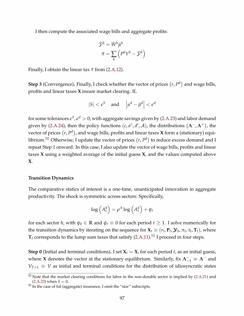
I then compute the associated wage bills and aggregate profits:

h = Whµh

π = ∑h

(PhYh − h

)Finally, I obtain the linear tax τ from (2.A.12).

Step 3 (Convergence). Finally, I check whether the vector of prices(r, Pd) and wage bills,

profits and linear taxes X insure market clearing. If,

|S| < εS and∣∣∣µd − µd

∣∣∣ < εd

for some tolerances εS, εd > 0, with aggregate savings given by (2.A.23) and labor demandgiven by (2.A.24), then the policy functions (c, a′,, d′,𝒜), the distributions

(Λ−, Λ+

), the

vector of prices(r, Pd), and wage bills, profits and linear taxes X form a (stationary) equi-

librium.52 Otherwise, I update the vector of prices(r, Pd) to reduce excess demand and I

repeat Step 1 onward. In this case, I also update the vector of wage bills, profits and lineartaxes X using a weighted average of the initial guess X, and the values computed aboveX.

Transition Dynamics

The comparative statics of interest is a one-time, unanticipated innovation in aggregateproductivity. The shock is symmetric across sectors. Specifically,

log(

Aht

)= ρA log

(Ah

t

)+ ψt

for each sector h, with ψ0 ∈ R and ψt ≡ 0 for each period t ≥ 1. I solve numerically forthe transition dynamics by iterating on the sequence for Xt ≡ (rt, Pt,Y t, πt, τt, Tt), whereTt corresponds to the lump sum taxes that satisfy (2.A.11).53 I proceed in four steps.

Step 0 (Initial and terminal conditions). I set Xt = X, for each period t, as an initial guess,where X denotes the vector at the stationary equilibrium. Similarly, fix Λ−

−1 ≡ Λ− and𝒱T+1 ≡ 𝒱 as initial and terminal conditions for the distribution of idiosyncratic states

52 Note that the market clearing conditions for labor in the non-durable sector is implied by (2.A.21) and(2.A.23) when S = 0.

53 In the case of ful (aggregate) insurance, I omit the “star” subscripts.

97

and the value function, where T denotes the horizon over which I compute the impulseresponses.

Step 1 (Households). First, I iterate backward on the functional equation (2.A.1)–(2.A.4),for each t ∈ 0, . . . , T, to obtain a sequence of policy functions ct, a′t, d′t,𝒜tt. Then, Iiterate forward on the transition kernel (2.A.5)–(2.A.6) using these policy functions, fort ∈ 0, . . . , T, to obtain a sequence of distributions

Λ−

t−1, Λ+t

t. Finally, I compute thesequence of aggregate demands for each goods

Yc

t , Ydt

t using (2.A.15)–(2.A.16).

Step 2 (Firms and market clearing). I iterate backward on (2.A.8)–(2.A.10), for t ∈ 0, . . . , T,to obtain the sequence of reset prices P?t t. Then, I iterate forward on (2.A.7) and (2.A.17)to obtain a new sequence of sectoral price indices54 Ptt and a sequence of TFP distor-sions Ωtt. Labor demands are computed from (2.A.18), using the sequence

Yc

t , Ydt

tfrom Step 1 and the initial sequence of prices Ptt. Finally, I compute new sequences forthe wage bills

Y t

t and aggreagte profits tt from (2.A.19)–(2.A.20).

Step 3 (Policy). I obtain new sequences for lump sum taxes Ttt and linear taxes τtt

from (2.A.11)–(2.A.12). Similarly, I compute the new sequence of nominal interest ratertt set by the monetary policy rule (2.A.13), given the price index (2.A.14).

Step 4 (Convergence). Finally, I check whether the sequence of endogeneous variablesXt ≡ (rt, Pt,Y t, πt, τt, Tt) insures market clearing. If,

‖x − x‖∞ < εx

for some tolerance εx > 0, for each sequence x ∈ r, P,Y , π, τ, T, then the policy func-tions ct, a′t, d′t,𝒜tt, the distributions

Λ−

t−1, Λ+t

t, and the prices and incomes Xtt forman equilibrium. Otherwise, I update the sequence Xtt using a weighted average of theinitial sequences Xtt and the new sequences Xtt

55 and I repeat Step 1 onward.

2.A.4 Calibration Strategy

The internal calibration consists of solving for the vectors of parameters(

β, ϑ, γ, B, Ad)— i.e. the discount factor, the preference parameter on non-durables, the (non-convex)

54 Again, to each set of initial conditions X corresponds a set of values for the same variables that satisfy theequilibrium restrictions. I denote these variables with a “bar”.

55 To insure convergence of the algorithm, the corresponding weights a decreasing exponentially in theperiod t.

98

durable adjustment cost, the supply of bonds, and the relative productivity in the durablesector — and prices

(r, Pd)— i.e. the real interest rate and the relative price of the durable

good at the stationary equilibrium — that solve the following restrictions: the two marketclearing conditions for labor (2.A.21); and the five empirical moments listed in Table 2.5.1.I proceed in two steps. First, I use the empirical targets and the restrictions in the model topin down the parameters

(Ad, B

)and the prices

(r, Pd). Then, I iterate over the remaining

parameters to insure market clearing, and match the rest of the targets.

Step 1. The first empirical moment in Table 2.5.1 directly pins down r. From (2.A.18) and(2.A.21),

µht ≡

(1

Ah Yht

) 11−α

(2.A.25)

for each sector h, at the stationary equilibrium. The second moment in Table 2.5.1 and(2.A.25) thus pin down Ad. Similarly, from (2.A.8),

Wh

Ph = Ah(

1 − αh) ε − 1

ε

(µh)−α

(2.A.26)

for each sector h. The last moment in Table 2.5.1 and (2.A.26) pin down Pd, given thenuméraire Pc ≡ 1 and the vector of productivities A previously solved for. Aggregateoutput js defined as

Y ≡ ∑h

PhYh with Yh = Ah(

µh)1−α

(2.A.27)

for each sector h, by definition of the production technologies. The fourth moment inTable 2.5.1 and (2.A.27) pin down B, given the vectors of prices P and productivities Aobtained above.

Step 2. Finally, I iterate on the remaining parameters (β, ϑ, γ) to satisfy the rest of therestrictions. Specifically, I adjust β until aggregate savings (2.A.23) are zero. Similarly, Iuse ϑ to clear the market for durable goods (2.A.21), with labor demand given by (2.A.16)and (2.A.18). Finally, I vary γ until the aggregate frequency of adjustment

𝒜T ≡ ∑h

µh∫

𝒜h (a, d, ζ) dΛh

matches the third moment in Table 2.5.1.

99

2.A.5 Numerical Implementation

I describe below the computation of the impulse responses in Section ??, and the numeri-cal implementation of the algorithms described in Appendices 2.A.3 and 2.A.3.

Grids and transition. The value functions are approximated on discrete grids for finan-cial assets and durable goods, consisting of 100 points each. The distribution of financialassets and durable goods is discretized on grids consisting of 300 points. I interpolatepolicy functions linearly between grid points, and use a generalization of Young (2010)’snon-stochastic stimuation method with multiple assets when using the policy functionsto iterate on the distribution of assets. For accuracy, the grid for financial assets is moredense in the neighborhood of the borrowing constraint. Finally, I discretize the incomeprocess on a 7-point grid using the method of Rouwenhorst (1995). I set T = 100 (quar-ters) when solving for the transition dynamics in general equilibrium (Section 2.6).

Numerical solution. The households’ problems (2.A.3)–(2.A.4) are non-convex due tofixed adjustment costs. To solve for the optimal policy, I first perform a grid search on afine grid to locate a candidate for the global maximum. I then use the gradient-free, sim-plex algorithm (Nelder-Meade) implemented in Matlab’s fminsearch to solve for a localoptimum, using this candidate as an initial condition. I use a tolerance of 10−5 to solvefor the value function at the stationary equilibrium, and one of 10−17 for the stationarydistribution (Step 1 in Appendix 2.A.3).

2.A.6 Complementary Numerical Results

In Section 2.6, I show that income redistribution affects the magnitude and the timingof the general equilibrium response of durable investment to productivity shocks. Fig-ure 2.A.1 plots the corresponding responses for non-durable consumption. There is nodiscernible pattern in this case, which highlights the role of lumpy and state-contingentadjustment for the response of durable spending.

100

Figure 2.A.1: Non-Durable Spending

No Redistribution Redistribution

2.B Omitted Proofs, Results and Derivations

2.B.1 Benchmark Case

In Section 2.3.2, I discuss a benchmark where the two goods are non-durable: δ = 1, i.e.full depreciation. In this case, no redistribution of labor income takes place across sectorsand there is no role for insurance from fiscal policy. For concision, no formal statement isprovided in the text. I do so in this section instead.

Proposition 2. Let Assumptions 4-5 hold. Consider a persistent, unanticipated productivityshock of the form (2.3.2), for any ψ0 ∈ R. Then, taxes under the insurance regime (2.2.11) satisfy:

T? = 0

Consequently, the response of durable investment satisfies:

Yd0

Yd =Yd,?

0Yd,?

for each period t ≥ 0, where Yd,(?)0 denotes aggregate durable investment (2.2.13) under the regimes

(2.2.10) and (2.2.11).

Proof of Proposition 2. First, I guess and verify that outputs in the economy without insur-ance (T ≡ 0) satisfy:

Yct

Yc =Yd

tYd (2.B.1)

101

By homotheticity,

cht (a, d, ζ) = c?t eh

t (a, d, ζ) and dh,′t (a, d, ζ) = d?t eh

t (a, d, ζ) (2.B.2)

with full depreciation. Here, (c?t , d?t ) denotes the (dual) cost-minimizing bundle thatachieves u (c, d′) ≥ 1, and eh

t (a, d, ζ) solves the following income fluctuations problem56:

Vht (a, ζ) = max

e,a′e1−σ

1 − σ+ βEt

[Vh

t+1(a′, ζ ′

)∣∣∣ ζ]

s.t. Pte + a′ ≤ (1 − τt) eht (ζ) + (1 + rt−1) a

a′ ≥ 0

where Pt denotes the CES ideal price index (2.A.14). In particular, (c?t , d?t ) is homogeneousof degree 0 in prices Pt.

From the firm’s price setting (2.A.8)–(2.A.10), the law of motion of price indices (2.A.7),the guess (2.B.1), and by Assumptions 4-5,

Pct

Pc =Pd

tPd (2.B.3)

so that (c?t , d?t ) = (c?, d?), i.e. the relative demand is unchanged compared to the station-ary equilibrium. Thus, the guess (2.B.1) is verified, from the market clearing conditions(2.A.15)–(2.A.16). The remaining equilibrium restrictions are satisfied.

Furthermore, note that:𝒴 c

tYc =

𝒴dt

Yd (2.B.4)

since wages are rigid, using the definitions of labor demands (2.A.17)–(2.A.18), and thewage bills (2.A.19). Then,

T?t = 0 (2.B.5)

under the regime with insurance, for each period t ≥ 0, by definition of taxes (2.A.11) andgiven the wage bills (2.B.4).

56 Note that the state variable d is redundant when δ = 1, and households do not incur a fixed costs whenadjusting their consumption of the good h = d.

102

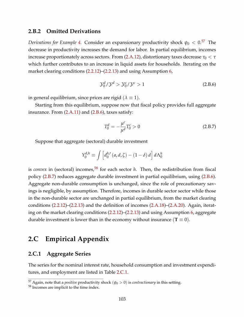
2.B.2 Omitted Derivations

Derivations for Example 4. Consider an expansionary productivity shock ψ0 < 0.57 Thedecrease in productivity increases the demand for labor. In partial equilibrium, incomesincrease proportionately across sectors. From (2.A.12), distortionary taxes decrease τ0 < τ

which further contributes to an increase in liquid assets for households. Iterating on themarket clearing conditions (2.2.12)–(2.2.13) and using Assumption 6,

𝒴d0 /𝒴d > 𝒴 c

0/𝒴 c > 1 (2.B.6)

in general equilibrium, since prices are rigid (λ ≡ 1).

Starting from this equilibrium, suppose now that fiscal policy provides full aggregateinsurance. From (2.A.11) and (2.B.6), taxes satisfy:

Td0 = −µc

µd Tc0 > 0 (2.B.7)

Suppose that aggregate (sectoral) durable investment

Yd,h0 ≡

∫ [dh,′

0 (a, d, ζ)− (1 − δ) d]

dΛh0

is convex in (sectoral) incomes,58 for each sector h. Then, the redistribution from fiscalpolicy (2.B.7) reduces aggregate durable investment in partial equilibrium, using (2.B.6).Aggregate non-durable consumption is unchanged, since the role of precautionary sav-ings is negligible, by assumption. Therefore, incomes in durable sector sector while thosein the non-durable sector are unchanged in partial equilibrium, from the market clearingconditions (2.2.12)–(2.2.13) and the definition of incomes (2.A.18)–(2.A.20). Again, iterat-ing on the market clearing conditions (2.2.12)–(2.2.13) and using Assumption 6, aggregatedurable investment is lower than in the economy without insurance (T ≡ 0).

2.C Empirical Appendix

2.C.1 Aggregate Series

The series for the nominal interest rate, household consumption and investment expendi-tures, and employment are listed in Table 2.C.1.

57 Again, note that a positive productivity shock (ψ0 > 0) is contractionary in this setting.58 Incomes are implicit to the time index.

103

Table 2.C.1: Data Sources

Series Seasonal Adjst Source

Nominal Interest Rate Fed Board H.15Effective Fed funds rate No (line 1)

Deflator NIPA 1.1.4.PCE Yes (line 2)

Personal Consumption Expenditures NIPA 1.1.3Real Yes (lines 4-6)

Residential Investment NIPA 1.1.3Real Yes (lines 14)

Employment CES (National)All employees Yes (see text)

Population NIPA 2.1Total No (line 40)

I define durable spending as the sum of household’s expenditures on durable goodsand residential investment. Non-durable spending consists of the sum of households’expenditures on non-durable goods and services, minus housing and financial / insur-ance services. I define durable-employment as the sum of employment in: construc-tion, durable manufacturing, wholesale trade and durable retail for durables, and repairand maintenance. Non-durable employment consits of the sum of employment in: non-durable manufacturing, wholesale trade and durable retail for durables, information, pro-fessional and business services, leisure and hospitality, and other services (except repairand maintenance). I exclude wholesale trade, retail trade (for data availability reasons)from either employment category. I exclude financial services and public administration.

2.C.2 PSID Data

In Section 2.4, I provide supporting evidence on the interaction between cyclical durableinvestment and redistribution. In particular, I confirm that labor income decreases pro-portionally more in durable sectors, compared to non-durable sectors, following a con-tractionary tax shock. To account for cross-sectoral labor mobility and movements in andout of the labor force, I use longitudinal data from the Panel Study of Income Dynamics(PSID).

Industry classification. Following Berger and Vavra (2015), I adopt a broad definition of

104

durable goods when calibrating the quantitative model in Section 2.5. This definitionincludes both consumer durables, and residential investment. Consistently, I classify in-dustries as either durable, or non-durable when using the PSID. Durable industries con-sists of construction, and durable manufacturing. Non-durable industries include non-durable manufacturing, and all services except public administration and the military,and finance59.

Income data. My preferred measure of incomes corresponds to (pre-tax) labor income, de-flated using a price index for total consumption expenditure. I also use family moneyincome to account for unemployment insurance and intra-household risk sharing.

Sample selection. I use the bi-annual PSID waves from 1968 to 201560. The sample consistsof male household’s heads aged 24-65. To eliminate outliers, I exclude households withlabor income lower than 5% of the annual average, and higher than the 95th percentile. Iuse PSID longitudinal weights.

2.C.3 Complementary Empirical Evidence

The measure of income that I use in the text is (real) labor income from the PSID. Forrobustness, I also use family income in to account for unemployment insurance and intra-household risk sharing. Figure 2.C.1 plots the corresponding series. The pattern is verysimilar: aggregate shocks lead to a redistribution of income between durable and non-durable workers.

59 Financial activities and real estate are inter-related, making their classification ambiguous. Public admin-istration and the military spending / employment have no immediate counterpart in my model. Exclud-ing these two industries is conservative with respect to the mechanism I am interested in since spendingand employment are less cyclical for these two industries than for private industries.

60 The industry classification in the PSID changed in 2017. I do not exploit this latest wage to avoid mea-surement issues.

105

Figure 2.C.1: Family Income (PSID)

Great Recession Response to Exogeneous Tax Increase


106


Alexopoulos, Michelle, “Read All about It!! What Happens Following a TechnologyShock?,” American Economic Review, June 2011, 101 (4), 1144–1179.

Alonso, Cristian, “Cutting Back on Labor Intensive Goods? Implications for Fiscal Stim-ulus,” Mimeo, Princeton November 2016.

Alvarez, Fernando, Francesco Lippi, and Juan Passadore, “Are State- and Time-Dependent Models Really Different?,” NBER Macroeconomics Annual, 2017, 31 (1), 379–457.

, , and Luigi Paciello, “Monetary shocks in models with observation and menu costs,”Journal of the European Economic Association, 05 2017, 16 (2), 353–382.

Attanasio, Orazio P., “Consumer Durables and Inertial Behaviour: Estimation and Ag-gregation of (S, s) Rules for Automobile Purchases,” Review of Economic Studies, 2000, 67(4), 667–696.

Auclert, Adrien, “Monetary Policy and the Redistribution Channel,” American EconomicReview, June 2019, 109 (6), 2333–2367.

Bachmann, Ruediger, Ricardo J. Caballero, and Eduardo M. R. A. Engel, “AggregateImplications of Lumpy Investment: New Evidence and a DSGE Model,” American Eco-nomic Journal: Macroeconomics, October 2013, 5 (4), 29–67.

Barsky, Robert, Christoph E. Boehm, Christopher L. House, and Miles Kimball, “Mon-etary Policy and Durable Goods,” Working Paper Series WP-2016-18, Federal ReserveBank of Chicago November 2016.

Basu, Susanto, John G. Fernald, and Miles S. Kimball, “Are Technology ImprovementsContractionary?,” American Economic Review, December 2006, 96 (5), 1418–1448.

Baxter, Marianne, “Are Consumer Durables Important for Business Cycles?,” The Reviewof Economics and Statistics, February 1996, 78 (1), 147–155.

107

Berger, David and Joseph Vavra, “Consumption Dynamics During Recessions,” Econo-metrica, January 2015, 83, 101–154.

Bertola, Giuseppe and Ricardo J. Caballero, “Kinked Adjustment Costs and AggregateDynamics,” in “NBER Macroeconomics Annual 1990, Volume 5” NBER Chapters, Na-tional Bureau of Economic Research, Inc, August 1990, pp. 237–296.

Bils, Mark and Peter J. Klenow, “Some Evidence on the Importance of Sticky Prices,”Journal of Political Economy, October 2004, 112 (5), 947–985.

, , and Benjamin A. Malin, “Testing for Keynesian Labor Demand,” NBER Macroeco-nomics Annual, 2013, 27 (1), 311–349.

Browning, Martin and Thomas F. Crossley, “Shocks, Stocks, and Socks: Smoothing Con-sumption Over a Temporary Income Loss,” Journal of the European Economic Association,December 2009, 7 (6), 1169–1192.

Buera, Francisco J. and Benjamin Moll, “Aggregate Implications of a Credit Crunch: TheImportance of Heterogeneity,” American Economic Journal: Macroeconomics, July 2015, 7(3), 1–42.

Caballero, Ricardo J., “Expenditure on Durable Goods: A Case for Slow Adjustment,”The Quarterly Journal of Economics, 1990, 105 (3), 727–743.

Caballero, Ricardo J, “Durable Goods: An Explanation for Their Slow Adjustment,” Jour-nal of Political Economy, April 1993, 101 (2), 351–384.

, “Notes on the Theory and Evidence on Aggregate Purchases of Durable Goods,” Ox-ford Review of Economic Policy, Summer 1994, 10 (2), 107–117.

Caballero, Ricardo J. and Eduardo M. R. A. Engel, “Explaining Investment Dynamicsin U.S. Manufacturing: A Generalized (S,s) Approach,” Econometrica, July 1999, 67 (4),783–826.

Caballero, Ricardo J, Eduardo M R A Engel, and John Haltiwanger, “Aggregate Employ-ment Dynamics: Building from Microeconomic Evidence,” American Economic Review,March 1997, 87 (1), 115–137.

Calvo, Guillermo A., “Staggered prices in a utility-maximizing framework,” Journal ofMonetary Economics, September 1983, 12 (3), 383–398.

108

Cantelmo, Alessandro and Giovanni Melina, “Monetary policy and the relative price ofdurable goods,” Journal of Economic Dynamics and Control, 2018, 86, 1 – 48.

Carroll, Christopher D and Miles S Kimball, “On the Concavity of the ConsumptionFunction,” Econometrica, July 1996, 64 (4), 981–992.

Carvalho, Carlos, “Heterogeneity in Price Stickiness and the Real Effects of MonetaryShocks,” The B.E. Journal of Macroeconomics, December 2006, 6 (3), 1–58.

Chari, V. V., Patrick J. Kehoe, and Ellen R. McGrattan, “Business Cycle Accounting,”Econometrica, May 2007, 75 (3), 781–836.

Christelis, Dimitris, Dimitris Georgarakos, Tullio Jappelli, Luigi Pistaferri, andMaarten van Rooij, “Asymmetric Consumption Effects of Transitory Income Shocks,”Economic Journal, 2019, 129 (622), 2322–2341.

Díaz, Antonia and María José Luengo-Prado, “The Wealth Distribution With DurableGoods,” International Economic Review, February 2010, 51 (1), 143–170.

Dynarski, Susan and Jonathan Gruber, “Can Families Smooth Variable Earnings?,”Brookings Papers on Economic Activity, 1997, 28 (1), 229–303.

Eberly, Janice C, “Adjustment of Consumers’ Durables Stocks: Evidence from Automo-bile Purchases,” Journal of Political Economy, June 1994, 102 (3), 403–436.

Floden, Martin and Jesper Lindé, “Idiosyncratic Risk in the United States and Sweden:Is There a Role for Government Insurance?,” Review of Economic Dynamics, July 2001, 4(2), 406–437.

Fuster, Andreas, Greg Kaplan, and Basit Zafar, “What Would You Do With $500? Spend-ing Responses to Gains, Losses, News and Loans,” NBER Working Papers 24386, Na-tional Bureau of Economic Research, Inc March 2018.

Guerrieri, Veronica and Guido Lorenzoni, “Credit Crises, Precautionary Savings, andthe Liquidity Trap,” The Quarterly Journal of Economics, 2017, 132 (3), 1427–1467.

Guvenen, Fatih, Sam Schulhofer-Wohl, Jae Song, and Motohiro Yogo, “Worker Betas:Five Facts about Systematic Earnings Risk,” American Economic Review, May 2017, 107(5), 398–403.

Hall, Robert E., “Investment, Interest Rates, and the Effects of Stabilization Policies,”Brookings Papers on Economic Activity, 1977, 8 (1), 61–122.

109

, “Job Loss, Job Finding, and Unemployment in the U.S. Economy over the Past FiftyYears,” NBER Macroeconomics Annual, 2005, 20, 101–137.

Heaton, John and Deborah Lucas, “Portfolio Choice in the Presence of Background Risk,”Economic Journal, January 2000, 110 (460), 1–26.

House, Christopher L., “Fixed costs and long-lived investments,” Journal of Monetary Eco-nomics, 2014, 68, 86 – 100.

Jaimovich, Nir, Sergio Rebelo, and Arlene Wong, “Trading down and the business cy-cle,” Journal of Monetary Economics, 2019, 102 (C), 96–121.

Johnson, David S., Jonathan A. Parker, and Nicholas S. Souleles, “Household Expendi-ture and the Income Tax Rebates of 2001,” American Economic Review, December 2006,96 (5), 1589–1610.

Kaplan, Greg, Benjamin Moll, and Giovanni L. Violante, “Monetary Policy Accordingto HANK,” American Economic Review, March 2018, 108 (3), 697–743.

, Kurt Mitman, and Giovanni L. Violante, “The Housing Boom and Bust: Model MeetsEvidence,” NBER Working Papers 23694, National Bureau of Economic Research, IncAugust 2017.

Kydland, Finn E and Edward C Prescott, “Time to Build and Aggregate Fluctuations,”Econometrica, November 1982, 50 (6), 1345–1370.

Loungani, Prakash and Richard Rogerson, “Cyclical fluctuations and sectoral realloca-tion : Evidence from the PSID,” Journal of Monetary Economics, March 1989, 23 (2), 259–273.

Mankiw, N. Gregory and Stephen Zeldes, “The consumption of stockholders and non-stockholders,” Journal of Financial Economics, 1991, 29 (1), 97–112.

Massa, Massimo and Andrei Simonov, “Hedging, Familiarity and Portfolio Choice,” TheReview of Financial Studies, 01 2006, 19 (2), 633–685.

McKay, Alisdair and Johannes F. Wieland, “Lumpy Durable Consumption Demand andthe Limited Ammunition of Monetary Policy,” April 2019.

, Emi Nakamura, and Jón Steinsson, “The Power of Forward Guidance Revisited,”American Economic Review, October 2016, 106 (10), 3133–3158.

110

Nakamura, Emi and Jón Steinsson, “Monetary Non-neutrality in a Multisector MenuCost Model,” The Quarterly Journal of Economics, 2010, 125 (3), 961–1013.

Ogaki, Masao and Carmen M. Reinhart, “Measuring Intertemporal Substitution: TheRole of Durable Goods,” Journal of Political Economy, October 1998, 106 (5), 1078–1098.

Parker, Jonathan A., Nicholas S. Souleles, David S. Johnson, and Robert McClelland,“Consumer Spending and the Economic Stimulus Payments of 2008,” American Eco-nomic Review, October 2013, 103 (6), 2530–2553.

Pastén, Ernesto, Raphael Schoenle, and Michael Weber, “The Propagation of MonetaryPolicy Shocks in a Heterogeneous Production Economy,” NBER Working Papers 25303,National Bureau of Economic Research, Inc November 2018.

Patterson, Christina, “The Matching Multiplier and the Amplification of Recessions,”Mimeo, MIT 2019.

Piazzesi, Monika and Martin Schneider, “Asset Prices and Asset Quantities,” Journal ofthe European Economic Association, 04-05 2007, 5 (2-3), 380–389.

Pistaferri, Luigi, “Why Has Consumption Remained Moderate after the Great Reces-sion?,” Mimeo, Stanford October 2016.

Ramey, Valerie A., “Identifying Government Spending Shocks: It’s all in the Timing,” TheQuarterly Journal of Economics, 2011, 126 (1), 1–50.

Romer, Christina D. and David H. Romer, “The Macroeconomic Effects of Tax Changes:Estimates Based on a New Measure of Fiscal Shocks,” American Economic Review, June2010, 100 (3), 763–801.

Rouwenhorst, Geert, Asset Pricing Implications of Equilibrium Business Cycle Models’, Vol.Chapter 10, Frontiers of Business Cycle Research, Princeton University Press, 1995.

Schulhofer-Wohl, Sam, “Heterogeneity and Tests of Risk Sharing,” Journal of PoliticalEconomy, 2011, 119 (5), 925–958.

Shapiro, Matthew D., “Investment, Output, and the Cost of Capital,” Brookings Papers onEconomic Activity, 1986, 17 (1), 111–164.

Skinner, Jonathan, “Risky income, life cycle consumption, and precautionary savings,”Journal of Monetary Economics, September 1988, 22 (2), 237–255.

111

Souleles, Nicholas S., “The Response of Household Consumption to Income Tax Re-funds,” American Economic Review, September 1999, 89 (4), 947–958.

Werning, Iván, “Incomplete Markets and Aggregate Demand,” NBER Working Papers21448, National Bureau of Economic Research, Inc August 2015.

Winberry, Thomas, “Lumpy Investment, Business Cycles, and Stimulus Policy,” AmericanEconomic Review, forthcoming 2019.

Young, Eric R., “Solving the incomplete markets model with aggregate uncertainty us-ing the Krusell-Smith algorithm and non-stochastic simulations,” Journal of EconomicDynamics and Control, January 2010, 34 (1), 36–41.

Zorzi, Nathan, “Lumpy Investment and the Non-Linear Response to Income Shocks,”Mimeo, MIT April 2020.

112

Chapter 3

Uninsured Income Risk and LaborMisallocation*

This paper explores how uninsured income risk can hinder the efficient matching betweenworkers and firms. I consider a model with two-sided heterogeneity between workers andoccupations. Workers are imperfectly insured against labor income risk due to incompletemarkets and borrowing constraints. In this setting, uninsured income risk induces labormisallocation across occupations, by reducing the incentives to search for the efficientmatch (ex ante) and by forcing excess separation (ex post). In turn, labor misallocation re-inforces endogeneously the effect of uninsured income risk, by depressing the value ofequity used for self-insurance. I quantify these mechanisms, how they depend on thestrength of assortative matching and the co-movements between occupations, and howthey affect households differentially depending on the strength of their comparative ad-vantage and across the wealth distribution. Finally, I assess the role of fiscal policy andsocial insurance in improving upon the laissez-faire allocation.

3.1 Introduction

In this paper, I explore how uninsured income risk can prevent an efficient assignmentof workers to occupations. I investigate this question using a variant of the Lucas andPrescott (1974) model augmented with two-sided heterogeneity between workers andoccupations and incomplete markets. In presence of liquidity constraints, workers arepotentially unable to search for and remain in occupations where they have a strongercomparative advantage. In this case, labor is misallocated across occupations, and there

* I thank Iván Werning, Ricardo Caballero, Marios Angeletos and Arnaud Costinot for helpful suggestions.All errors are my own.

113

is room for social insurance to help the workers overcome the financial frictions they face.

The benchmark model builds on the continuous-time setup of Alvarez and Shimer(2011), and extends it along two dimensions. The first novelty is that households andoccupations have permanent types, which allow for assortative matching. I am inter-ested in two distinct (and complementary) motives for sorting: either the productivityof the match is indexed by the worker’s and occupation’s types à la Becker (1973);1 orhouseholds and occupations differ in their risk tolerance and fundamental volatility, re-spectively.2 Job search takes both place off- and on-the-job, which generates a job ladder.3

The second novelty is that risk sharing is limited: worker- and occupation-specific incomerisk is uninsurable, and households face borrowing constraints.4 I set up the model suchthat complete markets allocation is efficient. As a result, any inefficient in the allocationof labor across occupations can be directly attributed to imperfect risk sharing.

Incomplete markets hinder the efficient assignment of workers to occupations throughtwo channels (Figure 3.1.1). First, imperfect risk sharing reduces workers’ incentives tosearch (ex ante) for a match where they have a stronger comparative advantage.5 In par-ticular, households shorten the average duration of their search, and settle inefficientlyfor occupations that are expanding or perceived as safer. These two effects are more pro-nounced for workers with a strong comparative advantage. Second, uninsured incomerisk and borrowing constraints induce excess reallocation (ex post) across occupations. Inpresence of incomplete markets and borrowing constraints, households have an ineffi-ciently high propensity to leave their occupation during a contraction. Workers sacri-fice their comparative advantage for the liquidity benefits of moving to another occupa-tion and improving their future income stream. This prediction is not uniform along the

1 Empirically, the idenfication of this form of assortative matching is complicated by the presence of searchfrictions (Eeckhout (2018) for a review). Multi-dimensional heterogeneity plays an important role in ex-plaining workers’ sorting across occupations as observed in the data (Lindenlaub and Postel-Vinay (2017);Guvenen et al. (2020); Postel-Vinay and Lise (2020)). For tractability reasons, I focus on uni-dimensionalheterogeneity, however.

2 Empirically, risk tolerant households sort into riskier occupations (Guiso et al. (2002), Bonin et al. (2007),Guiso and Paiella (2008) and Schulhofer-Wohl (2011)).

3 Job ladders are typically studied in search-theoretical frameworks (Burdett (1978); Moscarini and Postel-Vinay (2018)), as opposed to the Lucas and Prescott (1974) framework.

4 The evidence suggests that liquidity frictions shorten the workers’ job search (Chetty (2008)), reduce thequality of the resulting matches (Nekoei and Weber (2017)), and affect households’ occupational choicesby increasing the effective risk of some activities (Bianchi and Bobba (2012)).

5 It’s worth clarifying the terminology at this point. In the following, I suppose that there is hetero-geneity among workers (θ) and firms (θ?). The expected value (continuation value) of a match is log-supermodular in (θ, θ?), and symmetric in θ at the lower value for θ?. In the application with heteroge-neous productivities, I interpret θ as skill and θ? as skill-intensity. In the application with heterogeneity inrisk aversion and fundamental volatility, I interepret θ as risk tolerance and θ? as fundamental volatility.I refer to high θ households as having a (strong) comparative advantage.

114

wealth distribution when mobility entails a short-term liquidity cost. Workers with partic-ularly low liquidty buffers are unable to afford this mobility cost and can on the contraryhave an inefficiently low propensity to search for a new occupation.

These two channels interact and shape the workers’ income profiles. Compared to theefficient allocation, workers with a strong comparative advantage fall short on climbingtheir job ladder. This reduces their earnings, and the liquidity buffers they accumulate. Asa result, workers cycle excessively between occupations where they have a inefficientlylow comparative advantage. In particular, transitory income shocks can have very persis-tent effects.

Figure 3.1.1: Channels

ImperfectRisk Sharing

LaborMisallocation

Search (ex ante)+ Liquidity (ex post)

Wealth Inequality+ Excess Wage Volatility

ImperfectRisk Sharing

LaborMisallocation

Search (ex ante)

Lower Equity Value

+ Reallocation (ex post)

These effects are reinforced in general equilibrium (Figure 3.1.1). Labor misallocationdepresses aggregate productivity,6 which reduces the value of firms’ equity that house-holds use as liquidity buffer. This makes incomplete markets and borrowing constraintseven more acute, and reinforces labor misallocation.

I first illustrate these mechanisms qualitatively in a benchmark model. I then develop aquantitative version of this model to assess their importance. I enrich my setup along threedimensions. First, I introduce more realistic labor markets, with wage rigidites, searchfrictions and unvoluntary unemployment à la Blanchard and Galí (2010), and convex laboradjustment costs within occupations. Second, I allow for occupation-specific mobilitycosts, which I calibrate to replicate the pattern of gross and net flows observed in U.S.data. Third, I introduce worker-specific idiosyncratic income shocks to better match theempirical distribution of earnings.

Finally, I assess the role of fiscal policy in improving upon the laissez-faire allocation. Inparticular, I explore how unemployment insurance and severance payments allow house-holds to partially overcome the financial frictions that they face, and thus increase the

6 The literature has mostly studied credit frictions on the firms side as a source of labor misallocation(Restuccia and Rogerson (2008); Hsieh and Klenow (2009); Baqaee and Farhi (2020)). Instead, and I focuson the role of financial frictions on the households side.

115

quality of workers-occupations matches. However, these social insurance programs alsoraise the value of unemployment and discourage labor supply. I use my structural modelto solve for the optimal level and timing of unemployment insurance and severance pay-ments that trade-off between these forces.

The present version of the paper is very preliminary. The full analysis is presented inZorzi (2020b).

Related literature. My paper lies at the intersection of several strands of the literature onlabor mobility, assortative matching, incomplete markets and social insurance programs.

First, my paper contributes to an important literature on labor reallocation across sec-tors and occupations over the business cycle, in the tradition of Lucas and Prescott (1974).Alvarez and Shimer (2011) develop a tractable, continuous-time version of this model,which I build on. They assume complete markets and homogeneous workers, while I fo-cus precisely on incomplete markets and their implication for assortative matching. Fol-lowing Alvarez and Veracierto (2000) and Alvarez and Veracierto (2001), I explore the rolesocial insurance in the form of unemployment insurance and severance payments. Thepresence of occasionally-binding borrowing constraints in my setup creates a new motivefor front-loaded severance payments: they allow workers to partially undo the financialfrictions that they face in the short-term. Rogerson (2005) and Carrillo-Tudela and Vissch-ers (2014) augment the Lucas and Prescott (1974) model with sector-specific human capitalaccumulation over the life cycle.7 They assume that workers are risk neutral and abstractfrom their savings decision. Instead, I take worker’s schedule of comparative advantageas exogeneous, and I study whether uninsured income risk and borowing constraints af-fects their assignment to occupations.

Second, my paper fits into a large literature on assortative matching and the role oflabor market frictions in preventing an efficient assignment of workers to firms. Shimerand Smith (2000) study the conditions under which assortative matching is preserved inpresence of search frictions. Moscarini (2001) and Teulings and Gautier (2004) explorehow tight labor markets can disincentivize workers to search for occupations where theyhave a stronger comparative advantage.8 In turn, Marimon and Zilibotti (1999) and Fulleret al. (2014) investigate how unemployment insurance can improve the quality of worker-firm matches by raising the value of search. Lise et al. (2016) quantify this mechanism in

7 McLaughlin and Bils (2001) introduce assortative matching in a related multi-sector framework. Dvorkinand Monge-Nara (2019) allow for human capital accumulation in a dynamic, multi-sector general equi-librium model with labor mobility but focus on long-term growth (as opposed to cyclical fluctuations).

8 A similar mechanism is present in Acemoglu and Shimer (2000), though their focus is not explicitly onassortative matching.

116

a calibrated model with on-the-job search. My paper revisits this question in the contextof an heterogeneous agents model with occasionally-binding borrowing constraints.

Finally, my paper relates to a growing literature on labor supply and search in het-erogeneous agent, incomplete markets economies. Chang and Kim (2006) allow for anextensive margin of labor supply in an Aiyagari (1994) model. Krusell et al. (2010) in-troduce a frictional labor market and quantify optimal unemployment insurance in thissetting. Krusell et al. (2017) and Krusell et al. (2020) are interested in workers’ gross flowsbetween employment and unemployment. To the best of my knowledge, my paper is thefirst to embed the heterogeneous agents apparatus into a Lucas and Prescott (1974) modelwith occupation-specific risk.9 Furthermore, my focus on assortative matching is novel.

Layout. I start by introducing a benchmark multi-occupations, Lucas and Prescott (1974)economy with assortative matching and incomplete markets in Section 3.2. I investigatehow incomplete markets hinder the efficient assignment of workers to occupations in Sec-tion 3.3. Section 3.4 introduces a quantitative variant of this model. Section 3.5 discussesthe next steps.

3.2 Benchmark Model

The environment consists of a muti-occupations, Lucas and Prescott (1974) economy aug-mented with two features: assortative matching, and incomplete markets. There is a con-tinuum of labor markets, corresponding to various occupations. The product of these oc-cupation is used as intermediary input in a final good sector. Occupations are subject toidiosyncratic demand shocks, while the final good sector is not. Mobility between thelabor markets entails a liquidity cost. The economy is inhabited by a continuum of house-holds who consume, save, supply labor in their occupation10 and move between those.Households and occupations are indexed by permanent types, allowing for assortativematching. Households face incomplete markets and borrowing constraints, which is theonly source of inefficiency in this economy. I introduce the environment in Section 3.2.1. Istate the market clearing conditions in Section 3.2.2. Section 3.2.3 discusses some proper-ties of the model.

9 In separate work (Zorzi (2020a)), I study the role of income redistribution in a multi-sector, heterogeneousagents economy. However, I rule out labor mobility between sectors, and I abstract from unemployment.

10 There is no unvoluntary unemployment in this benchmark model. I address this question the richermodel presented in Section 3.4.

117

3.2.1 Environment

Time is continuous, and there is no aggregate uncertainty.11 Periods are indexed by t ≥ 0.

Occupations. A continuum of occupations produces intermediary inputs. Each occupa-tion admits a representative firm. Occupations are characterized by three idiosyncraticstates: their permanent type (θ?), their idiosyncratic demand shifter (ϕ), and the distribu-tion of idiosyncratic states for households located in this occupation (Λ).12 Firms’ typesθ? lie in some continuum Θ. In the following, I let z? ≡ (θ?, ϕ, Λ) denote the vector ofoccupations’ idiosyncratic states, and π denote the associated measure.

The representative firm in each occupation has access to a linear technology f : n ↦→ben for some be > 0, where n denotes effective labor demand. Prices are flexible in theseoccupations and firms are competitive.

Final goods sector. A final goods producer combines the output of the various occupa-tions:13

Q =

[∫exp (ϕ)

1ν y (z?)

ν−1ν dπ

] νν−1

(3.2.1)

where ϕ denotes (stochastic) demand shifters and y (z?) denotes demand for input pro-duced by the occupations. The final good producer is competitive and its price is nor-malized to 1 (numéraire). The demand shifters follow a first-order autoregressive process,which is indexed by the occupation’s type θ?. Specifically,

dϕt = −η (ϕt − ϕ) dt + σθ?Bt (3.2.2)

for some (common) mean and persistence ϕ > 0 and η > 0, and some type-specific volatil-ity σθ? ≥ 0, where Bt denotes a (standard) Wiener process, with independence across oc-cupations.

Households. The economy is inhabited by of a continuum of mass 1 of households. Eachhousehold is indexed by five idiosyncratic states: their permanent type (θ), their financialasset holdings (a), their mobility status (m), their mobility cost (λ), and the set of idiosyn-cratic states characterizing the occupation they are located in (z?). Households’ types θ

11 I focus on the properties of the stationary equilibrium of this economy.12 Specifically, Λ corresponds to the distribution of (θ, a, m, λ) (defined below) in the relevant occupation.13 The exogeneous process for demand shifters is normalized so that

∫exp (ϕ) dπ ≡ 1, i.e. ϕ =

− log∫

exp(

14

σ2θ?

ρ

)dπ? using the notation introduced below, where π? ≡ margθ?π.

118

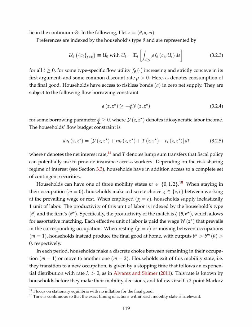
lie in the continuum Θ. In the following, I let z ≡ (θ, a, m).

Preferences are indexed by the household’s type θ and are represented by

𝒰θ

(ctt≥0

)≡ U0 with Ut = Et

[∫s≥t

ρ fθ (cs, Us) ds]

(3.2.3)

for all t ≥ 0, for some type-specific flow utility fθ (·) increasing and strictly concave in itsfirst argument, and some common discount rate ρ > 0. Here, ct denotes consumption ofthe final good. Households have access to riskless bonds (a) in zero net supply. They aresubject to the following flow borrowing constraint

a (z, z?) ≥ −φ𝒴 (z, z?) (3.2.4)

for some borrowing parameter φ ≥ 0, where 𝒴 (z, z?) denotes idiosyncratic labor income.The households’ flow budget constraint is

dat (z, z?) = [𝒴 (z, z?) + rat (z, z?) + T (z, z?)− ct (z, z?)] dt (3.2.5)

where r denotes the net interest rate,14 and T denotes lump sum transfers that fiscal policycan potentially use to provide insurance across workers. Depending on the risk sharingregime of interest (see Section 3.3), households have in addition access to a complete setof contingent securities.

Households can have one of three mobility states m ∈ 0, 1, 2.15 When staying intheir occupation (m = 0), households make a discrete choice χ ∈ e, r between workingat the prevailing wage or rest. When employed (χ = e), households supply inelastically1 unit of labor. The productivity of this unit of labor is indexed by the household’s type(θ) and the firm’s (θ?). Specifically, the productivity of the match is ζ (θ, θ?), which allowsfor assortative matching. Each effective unit of labor is paid the wage W (z?) that prevailsin the corresponding occupation. When resting (χ = r) or moving between occupations(m = 1), households instead produce the final good at home, with outputs bu > bm (θ) >

0, respectively.

In each period, households make a discrete choice between remaining in their occupa-tion (m = 1) or move to another one (m = 2). Households exit of this mobility state, i.e.they transition to a new occupation, is given by a stopping time that follows an exponen-tial distribution with rate λ > 0, as in Alvarez and Shimer (2011). This rate is known byhouseholds before they make their mobility decisions, and follows itself a 2-point Markov

14 I focus on stationary equilibria with no inflation for the final good.15 Time is continuous so that the exact timing of actions within each mobility state is irrelevant.

119

process on λ0, λ1, with λ0 > 0 and λ1 = 0.16 I denote the transition rates between thesetwo states by s0, s1 > 0, respectively. When exiting the mobility state, households drawan idiosyncratic state z? from its stationary distribution, i.e. search is random. At thatpoint, they have the choice between entering this occupation (m = 2) or keep searchingfor another one (m = 1). When entering an occupation, households enter an intermediarystatus (m = 2) in which they are not allowed to rest.17 They exit this temporary status andbecome regular workers (m = 0) with a rate s2 > 0.

Summing up, labor incomes satify:

𝒴 (z, z?) =

ζ (θ, θ?)W (z?) if m = 0, χ = e or m = 2

bu if m = 0, χ = r

bm (θ) if m = 1

(3.2.6)

Labor markets. Labor markets are frictionless in this benchmark environment. I allow forsearch frictions and unvoluntary empoyment within occupations in Section 3.4.

3.2.2 Equilibrium

Occupations. The good and labor market clearing conditions in each occupation are

y (z?) = be∫ ∫

1χ(z)=eζ (θ, θ?)Λ (dz, z?) dπ (3.2.7)

for some productivity be > 0.

Final good. The market clearing condition for the final goods is∫c (z, z?)Λ (dz, z?) dπ = Q +

∫ [bu1χ(z)=u + bm1m=1

]Λ (dz, z?) dπ (3.2.8)

Recursive equilibrium. A recursive equilibrium is defined as usual. It consists of valuefunctions and policy functions for households, indexed by (z, z?), for consumption, sav-ings, labor supply and mobility such that households maximize (3.2.3) subject to (3.2.4)–(3.2.6), firms choose intermediary inputs optimally, and market clearing conditions (3.2.7)–(3.2.8) together with (3.2.1). In the following, I focus on the stationary equilbrium of thiseconomy, i.e. aggregate quantities and prices are constant over time.

16 That is, some households are unable to move across occupations even if they wanted to, for reasonsoutside the scope of this model. I discuss the role of this assumption in Section 3.2.3.

17 That is, households cannot become unemployed and generate bu until they have worked for a sufficientlong period of time in this occupation.

120

3.2.3 Discussion

Before exploring how incomplete markets affect the matching betweeen workers andfirms, I discuss some of the modelling choices.

Efficiency. The complete markets equilibrium is efficient, as in Alvarez and Shimer (2011).This property allows me to attribute any deviation from the first best allocation, i.e. labormisallocation across occupations, to imperfect risk sharing.

Assortative matching. I allow for two distinct sources of sorting. First, I let the pro-ductivity of the worker-occupation match depend on their types. Specifically, I assumethat ζ (θ, θ?) is log-supermodular as in Becker (1973). An extensive literature studies howsuch complementarity between workers and firms affects the allocation of labor acrossoccupations, both in efficient environments18 and in presence of search frictions.19 I aminterested in the role of imperfect risk in preventing workers to exploit efficiently theircomparative advantage. Second, I allow households and occupations to differ in their risktolerance and fundamental volatility, respectively. Specifically, I suppose that households’flow utility fθ belong to the Epstein and Zin (1989) class, with type-specific risk aversionsγθ > 0 but a common (inverse) elasticity of substitution σ > 0.20 The literature on theeffect of risk aversion and liquidity frictions on labor supply and occupational choice ismostly empirical.21,22 My framework allows me to explore whether incomplete marketsand borrowing constraints discourage workers from seeking employment in risky occu-pations, by increasing the effective risk of being employed in those. When parametrizedwithout assortative matching and complete markets, my model reduces down to Alvarezand Shimer (2011), with the exception that occupations are subject to demand shocks in-stead of productivity shocks.

18 See Acemoglu and Autor (2011) and Costinot and Vogel (2015) for reviews of the literature.19 See Eeckhout (2018) for a survey.20 That is, is set fθ (c, U) = ρ

1−σ

(u?θ c1−σ − ((1 − γθ)U)

1−σ1−γθ

)/(((1 − γθ)U)

γθ−σ1−γθ

)(Duffie and Epstein

(1992)), for some coefficients

u?θ

θ∈Θ. I set these coefficients such that fθ (c?,𝒰θ) = fθ′ (c?,𝒰θ′), foreach pair of types (θ, θ′). Here, c? denotes consumption in the complete markets, stationary equilibrium,and 𝒰θ solves (3.2.3).

21 For empirical references, see footnote 2.22 A large literature investigates the role of preferences towards risk and borrowing constraints on en-

trepreneurial choice (Kihlstrom and Laffont (1979), Evans and Jovanovic (1989) and Vereshchagina andHopenhayn (2009)). However, an occupational choice differs from an entrepreneurial choice in variousrespects. In particular, the degree of uninsurable income risk and the importance of financial frictions arepotentially very different in these two contexts.

121

Mobility costs. Mobility across occupations entails two types of cost in my model. First,households face a short-term liquidity cost in the form of non-employment with bene-fits bm < bu while transitioning (stochastically) between occupations at rate λ0. Second,households incur an opportunity cost in the form of foregone earnings if they leave anoccupation where they have a strong comparative advantage. In presence of incompletemarkets and borrowing constraints, the timing of these costs is relevant. As I discuss inSection 3.3.4, two pairs (bm, λ0) with the same cost in present discounted value can havevery different implications for the pattern of labor reallocation across occupations whenrisk sharing is imperfect. In particular, liquidity costs play an important role when house-holds are unable to relocate in the short-term, i.e. when the transition rate s0/s1 is high.In this case, households drawn down their liquidity buffer after a contractionary shockbefore being able to relocate, making the liquidity cost potentially prohibitive.

Model reduction. As noted in Section 3.2.1, each occupation is indexed by two scalars, i.e.its type (θ?) and demand shifter (ϕ), and a distribution of households’ idiosyncratic states(Λ). With a continuum of occupations, a (stationary) equilibrium involves a distributionof such distributions. The dimensionality of this object large. To circumvent this issue, thedistributions Λ can be parametrized by a finite vector Λ?.23 In the following, I use Λ andΛ? interchangeably.

3.3 Risk Sharing and Efficiency

I am interested in the role of risk sharing (or the lack thereof) for the households’ alloca-tion across occupations. Specifically, I consider two risk sharing regimes and I comparetheir positive and normative implications. I start with a full insurance, complete marketsbenchmark.24 I then allow for imperfect risk sharing. Specifically, I suppose that fiscalpolicy can provide partial insurance in the form of lump sum transfers.25 I parametrizethese transfers so they nest the two polar cases of full insurance and no insurance, and Iperform a comparative statics with respect to this parameter.

23 Algan et al. (2008) and Fernández-Villaverde et al. (2019) propose alternative approaches, among others.24 Formally, households contract on contingent securities in an ex ante period (with no endowments). Then,

they are assigned randomly (and independently) across idiosyncratic states according to some measuresπ?. In turn, these idiosyncratic states evolve as described above. This yields a stationary distributionwith measures π. Households form rational expectations when contracting, i.e. I am interested in thefixed point π? = π.

25 In Section 3.4, I explicitly model unemployment insurance and severance payments in a model withfrictional labor markets.

122

3.3.1 Assumptions

I specialize the environment presented in Section 3.2.1 in two respects. First, I focus ex-clusively on comparative advantage in this version of the paper. That is, I abstract fromheterogeneity in risk tolerance and fundamental volatility across workers and occupa-tions, respectively. For simplicity, I suppose that the inverse elasticity of intertemporalsubstitution (σ) and risk aversions (γθ) coincide, so that utility is separable:

U0 = E0

[∫u (ct) dt

], u (c) ≡ c1−σ

1 − σ

Assumption 7. γθ = σ > 0, for each households’ type θ ∈ Θ, and σθ? = σ? > 0, for eachoccupations’ type θ? ∈ Θ.

Second, I suppose that workers with a stronger comparative advantage in high θ? oc-cupations are also more productive. Specifically, I assume that households are uniformlyproductive in the lowest θ? occupation. In other words, θ captures the workers’ skill andθ? the occupations’ skill-intensity. Skilled workers have both an absolute advantage, anda comparative advantage in high θ? occupations. Furthermore, I suppose that the sched-ule of benefits while moving bm (θ) insures that the value of unemployment V (θ) undercomplete markets (Section 3.3.2) is not indexed by the households’ type. Put it differently,high skill workers have a higher cost of retraining when moving between occupations.This assumption rules out on-the-job search with complete markets.26

Assumption 8. ζ (θ, θ?0) = ζ (θ′, θ?0), for each pair (θ, θ′), where θ?0 ≡ inf Θ, and bm (θ) ischosen such that V (θ) = V0, for each households’ type θ ∈ Θ, with V (θ) defined in (3.3.5).

3.3.2 Complete Markets

This economy is frictionless, so that the complete markets equilibrium is efficient. I thuscharacterize it as the solution to the planner’s problem.27 Households’ idiosyncratic statesreduce to z ≡ (θ, m) and z?, with a slight abuse of notation.

Planner’s problem. For reference, I state the planner’s problem in Appendix 3.A. At op-timum, the planner’s problem reduces to solving for a drift 𝜇 (z?) and a volatility 𝜎 (z?)for the occupations’ idiosyncratic states, an associated distribution g (z?), the type-specific

26 As discussed in Section 3.3.3, on-the-job search potentially takes places with incomplete markets. Simi-larly, on-the-job search occurs in the richer model I introduce in Section 3.4, regardless of the degree ofrisk sharing.

27 This approach parallels Alvarez and Shimer (2011).

123

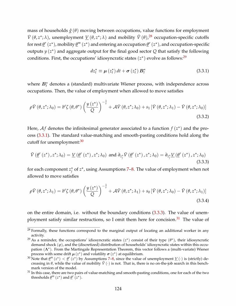
mass of households g (θ) moving between occupations, value functions for employmentV (θ, z?; λ), unemployment V (θ, z?; λ) and mobility V (θ),28 occupation-specific cutoffsfor rest θr (z?), mobility θm (z?) and entering an occupation θe (z?), and occupation-specificoutputs y (z?) and aggregate output for the final good sector Q that satisfy the followingconditions. First, the occupations’ idiosyncratic states (z?) evolve as follows:29

dz?t ≡ 𝜇 (z?t ) dt + 𝜎 (z?t )𝐵?t (3.3.1)

where 𝐵?t denotes a (standard) multivariate Wiener process, with independence across

occupations. Then, the value of employment when allowed to move satisfies

ρV (θ, z?; λ0) = beζ (θ, θ?)

(y (z?)

Q

)− 1ν

+𝒜V (θ, z?; λ0) + s1 [V (θ, z?; λ1)− V (θ, z?; λ0)]

(3.3.2)

Here, 𝒜 f denotes the infinitesimal generator associated to a function f (z?) and the pro-cess (3.3.1). The standard value-matching and smooth-pasting conditions hold along thecutoff for unemployment:30

V (θr (z?) , z?; λ0) = V (θr (z?) , z?; λ0) and ∂z?jV (θr (z?) , z?; λ0) = ∂z?j

V (θr (z?) , z?; λ0)

(3.3.3)

for each component z?j of z?, using Assumptions 7–8. The value of employment when notallowed to move satisfies

ρV (θ, z?; λ1) = beζ (θ, θ?)

(y (z?)

Q

)− 1ν

+𝒜V (θ, z?; λ1) + s0 [V (θ, z?; λ0)− V (θ, z?; λ1)]

(3.3.4)

on the entire domain, i.e. without the boundary conditions (3.3.3). The value of unem-ployment satisfy similar restructions, so I omit them here for concision.31 The value of

28 Formally, these functions correspond to the marginal output of locating an additional worker in anyactivity.

29 As a reminder, the occupations’ idiosyncratic states (z?) consist of their type (θ?), their idiosyncraticdemand shock (ϕ), and the (discretized) distribution of households’ idiosyncratic states within this occu-pation (Λ?). From the Martingale Representation Theorem, this vector follows a (multi-variate) Wienerprocess with some drift 𝜇 (z?) and volatility 𝜎 (z?) at equilibrium.

30 Note that θm (z?) < θr (z?) by Assumptions 7–8, since the value of unemployment V (·) is (strictly) de-creasing in θ, while the value of mobility V (·) is not. That is, there is no on-the-job search in this bench-mark version of the model.

31 In this case, there are two pairs of value-matching and smooth-pasting conditions, one for each of the twothresholds θm (z?) and θr (z?).

124

mobility satisfies

ρV (θ) = bm (θ) + λ0

∫max

V? (θ, z?)− V (θ) , 0

dg (3.3.5)

where the value of joining of new occupation is

ρV? (θ, z?) = beζ (θ, θ?)

(y (z?)

Q

)− 1ν

+𝒜V? (θ, z?) + s2

∫[V (θ, z?)− V? (θ, z?)] dg

(3.3.6)The threshold for entering an occupation satisfies

V? (θe (z?) , z?) = V (θe (z?)) (3.3.7)

In turn, the thresholds for unemployment θr (z?) and mobility θm (z?), together with(3.3.1), induce a drift 𝜇′ (z?) and a volatility 𝜎′ (z?), a distribution of occupations’ id-iosyncratic states g′ (z?) a type-specific mass of households g′ (θ) moving between occu-pations.32 The fixed point requirements are

𝜇′ (z?) = 𝜇 (z?) , 𝜎′ (z?) = 𝜎 (z?) , g′ (z?) = g (z?) , g′ (θ) = g (θ) (3.3.8)

Finally, occupation-specific outputs satisfy

y (z?) = be∫ ∫

1θ≥θr(z?)ζ (θ, θ?)Λ (dz, z?) dg, (3.3.9)

and total output produced by the final good sector is defined as

Q ≡[∫

exp (ϕ)1ν y (z?)

ν−1ν dπ

] νν−1

(3.3.10)

Labor allocation. This model is one of efficient allocation and reallocation of labor acrossoccupations. As occupations are hit by demand shocks, the households with low com-parative advantage in those occupations become unemployed (θ ≤ θr (z?)). Ultimately,those with the lowest comparative advantage (θ ≤ θm (z?)) leave the occupation alto-gether. They search for a new activity, and are allocated (stochastically) to one. Thisprocess repeats itself until households are assigned to an occcupation where they have asufficiently strong comparative advantage. At this point, they have a lower propensity toleave this occupation as it is subject to subsequent demand shocks. Crucially, this efficient

32 For the reason discussed in Section 3.2.3, the dimensionality of g (z?) is large so that the associated flowequations are untractable. Instead, I approximate numerically these distributions by simulating the evo-lution of a large number of occupations.

125

allocation is supported by full risk sharing. The underlying payments insure that house-holds have the proper incentives to search for a better occupation, and enough liquidityto remain in those as they are hit by demand shocks. From Section 3.3.3 on, I relax theassumption of complete markets and I explore how imperfect risk sharing affects theseincentives and whether it contributes to labor misallocation across occupations.

Implementation. I supposed so far that households were able to contract (ex ante) on acomplete set of contingent securities. Alternatively, the allocation characterized above canbe implemented by lump sum transfers from fiscal policy T (z, z?).33 These payments in-sure that households’ total income (including tranfers) is constant over time, which allowsthem to perfectly smooth out consumption across periods and (idiosyncratic) states. Taxdifferentials satisfy

T (z, z?)− T(z′, z?,′) = 𝒴

(z′, z?,′)−𝒴 (z, z?) (3.3.11)

for each pairs of households’ idiosyncratic states (z, z?) and (z′, z?,′). In turn, incomes aregiven by (3.2.6) with

W (z?) = be(

y (z?)Q

)− 1ν

(3.3.12)

at equilibrium. Finally, the level of taxes is pinned down by∫T (z, z?) dΛdπ = 0 (3.3.13)

These restrictions allow to solve for the contingent transfers T (z, z?). I use these transfersto parametrize the degree of risk sharing when markets are incomplete.

3.3.3 Incomplete Markets

I now assume that markets are incomplete. I investigate whether imperfect risk sharingcan hinder the efficient allocation of labor across occupations. In presence of incompletemarkets, the distribution of financial assets becomes relevant. That is, households’ id-iosyncratic states are z ≡ (θ, a, m) and z?.

Insurance. I allow fiscal policy to provide partial insurance in the form of lump sum

33 Formally, these payments should be indexed by the households’ permanent type and the entire history ofshocks they are subject to, i.e. occupation-speific demand shocks, idiosyncratic mobility costs and theirdraws when moving between occupations. As is apparent from (3.3.11)–(3.3.13), households’ currentidiosyncratic states (z, z?) is a sufficient statistics for these payments.

126

transfers. However, these payments do not fully undo the financial frictions faced by thehouseholds. These transfers serve two purposes. First, they allow me to parametrize thedegree of risk sharing in my economy, and explore how the efficiency of the allocationof labor changes as the market incompleteness becomes more acute. Second, they cap-ture in reduced form various social insurance policies, i.e. unemployment insurance andseverance payments. I explicitly model those from Section 3.4 on.

When assessing the role of imperfect risk sharing, I am interested in the channelsthrough which it operates. In particular, I disentangle between uninsurable income changesthat are specific to a household’s current occupation or idiosyncratic to her. For this reason,I parametrize these transfers as follows:

T′ (z, z?) = ψ [T (z, z?)− T? (θ, z?)]︸︷︷︸Idiosyncratic insurance

+ψ? T? (θ, z?)︸︷︷︸Aggregate insurance

−T (3.3.14)

for each pair of households’ idiosyncratic states (z, z?), given some loadings ψ, ψ? ∈ [0, 1].The second term in (3.3.14),

T? (θ, z?) ≡∫𝒮(θ)

T (z, z?)Λ (dz, z?) (3.3.15)

with 𝒮 (θ) ≡ (z, z?)| z = (θ, a, m) for some a, m, allows fisal policy to provide aggregateinsurance, by insulating households against shocks affecting the occupations they workin (fixing a households’ type). The first term, allows fiscal policy to insure householdsagainst the history of their idiosyncratic shocks. In particular, the model replicates thecomplete markets when setting ψ = ψ?. Finally, T insures that∫

T′ (z, z?) dΛdπ = 0 (3.3.16)

Equilibrium. A recursive equilibrium in this economy consists of a drift 𝜇 (z?) and avolatility 𝜎 (z?) for the occupations’ idiosyncratic states, a distribution of occupations’idiosyncratic states g (z?), the type-specific mass of households g (θ, a) moving betweenoccupations, value functions for employment V (θ, a, z?; λ), unemployment V (θ, a, z?; λ)

and mobility V (θ, a),34 occupation-specific cutoffs for rest θr (a, z?) and mobility θm (a, z?),sectoral output y (z?) and aggregate ouput produced by the final good sector Q, andlump sum transfers T′ (z, z?) that satisfy the following conditions. Transfers are givenby (3.3.14)–(3.3.16). The occupations’ idiosyncratic states (z?) still evolve as (3.3.1), re-

34 Contrary to the complete markets case, these functions now correspond to the value functions (in level)associated to each activity.

127

gardless of the degree of risk sharing. The associated fixed point requirements (3.3.8) areunchanged, and so is the definition of occupation-specific output (3.3.9) and aggregateoutpout produced by the final good sector (3.3.10). The only difference between theseeconomies lies in households’ decisions (and the distributions they induce). For the sakeof notation, the expressions below implicitly assume that the cutoffs satisfy θm (a, z?) <θr (a, z?) as in the complete markets allocation, i.e. there is no on-the-job search. Thisis not necessarily the case at equilibrium, as discussed in Section 3.3.4.35 The value ofemployment when allowed to move satisfies

ρV (θ, a, z?; λ0) = maxc

u (c) +𝒜ecV (θ, a, z?; λ0) + s1 [V (θ, a, z?; λ1)− V (θ, a, z?; λ0)]

(3.3.17)

Here, 𝒜ec f denotes the infinitesimal generator associated to a function f (z?), the process

(3.3.1) and the savings rate (3.2.5) with 𝒴 (z, z?) = beζ (θ, θ?)(

y(z?)Q

)− 1ν . Again, the stan-

dard value-matching and smooth-pasting conditions hold along the cutoff for unemploy-ment:

V (θr (a, z?) , a, z?; λ0) = V (θr (a, z?) , a, z?; λ0)

and ∂z?jV (θr (a, z?) , a, z?; λ0) = ∂z?j

V (θr (a, z?) , a, z?; λ0) (3.3.18)

for each component z?j of z?. In addition, the borrowing constraint (3.2.4) acts as a reflect-ing barrier:

∂aV (θ, a, z?; λ0) ≥ u′(𝒴 (z, z?)− rφ𝒴 (z, z?) + T (z, z?)

)(3.3.19)

The values of employment when not allowed to move satisfies

ρV (θ, a, z?; λ1) = maxc

u (c) +𝒜ecV (θ, a, z?; λ1) + s0 [V (θ, a, z?; λ0)− V (θ, a, z?; λ1)]

(3.3.20)

Boundary conditions of the form (3.3.18) do not apply, while one of the form (3.3.19) does.The value of unemployment satisfy similar restrictions, so I omit them here for concision.Finally, the value of mobility satisfies

35 Numerically, this requires to: (i) guess a sequence of cutoffs defining regions for unemployment andmobility; (ii) solve for the value functions, given this guess, and compare the values of unemploymentand mobility to determine the regions over which unemployment and mobility are optimal; and (iii)update the guess until the regions coincide. The richer model introduced in Section 3.4 circumvents thisissue by assuming that unemployment is unvoluntary.

128

ρV (θ, a) = maxc

u (c) +𝒜m

c V (θ, a) + λ0

∫max

V? (θ, a, z?)− V (θ, a) , 0

dg

(3.3.21)here 𝒜m

c f denotes the infinitesimal generator associated to a function f (z?), the process(3.3.1) and the savings rate (3.2.5) with 𝒴 (z, z?) = bm (θ). The value of joining a newoccupation is

ρV? (θ, a, z?) = maxc

u (c) +𝒜e

cV? (θ, a, z?) + s2

∫[V (θ, a, z?)− V? (θ, a, z?)] dg

(3.3.22)

The threshold for entering an occupation satisfies

V? (θe (a, z?) , a, z?) = V (θe (a, z?, a) , a) (3.3.23)

Again, a boundary condition of the form (3.3.19) applies.Not surprisingly, (3.3.17)–(3.3.23) are equivalent to (3.3.2)–(3.3.7) when setting ψ =

ψ? = 1, i.e. with complete markets. In this case, households are provided with enoughliquidity to insure that their incentives to search across occupations and remain in themcoincide with the planner’s. Therefore, the equilibrium allocation is efficient. Away fromthis benchmark, households’ incentives do not necessarily line up with the planner’s. Inparticular, the cutoff for mobility θm (a, z?) is now indexed by the households’ holdingsof financial assets. Imperfect risk sharing leads to an inefficient dispersion in the house-holds’ financial asset holdings (a). In turn, this creates room for labor misallocation acrossoccupations.36

3.3.4 Labor Misallocation

To understand how incomplete markets and borrowing constraints affect the household’smobility decisions, I consider the following two partial equilibrium experiments.37 Thefirst one illustrates how incomplete markets affect households’ incentives to search acrossoccupations. The second one illustrates how it affects their incentives to leave an occupa-tion when this activity is subject to demand shocks.

Inefficient search (ex ante). The first experiment focuses on households’ search. It consistsof one-time, unanticipated mean preserving spread in the distribution of liquid financial

36 I focus here on the mobility decision. However, incomplete markets also affect the labor supply decision,i.e. the choice between employment and unemployment, even absent mobility.

37 In particular, I implicitly fix the drift 𝜇 (z?) and volatility 𝜎 (z?), the aggregate distributions g (z?) andg (θ, a), and outputs y (z?) and Q at their (general) equilibrium levels.

129

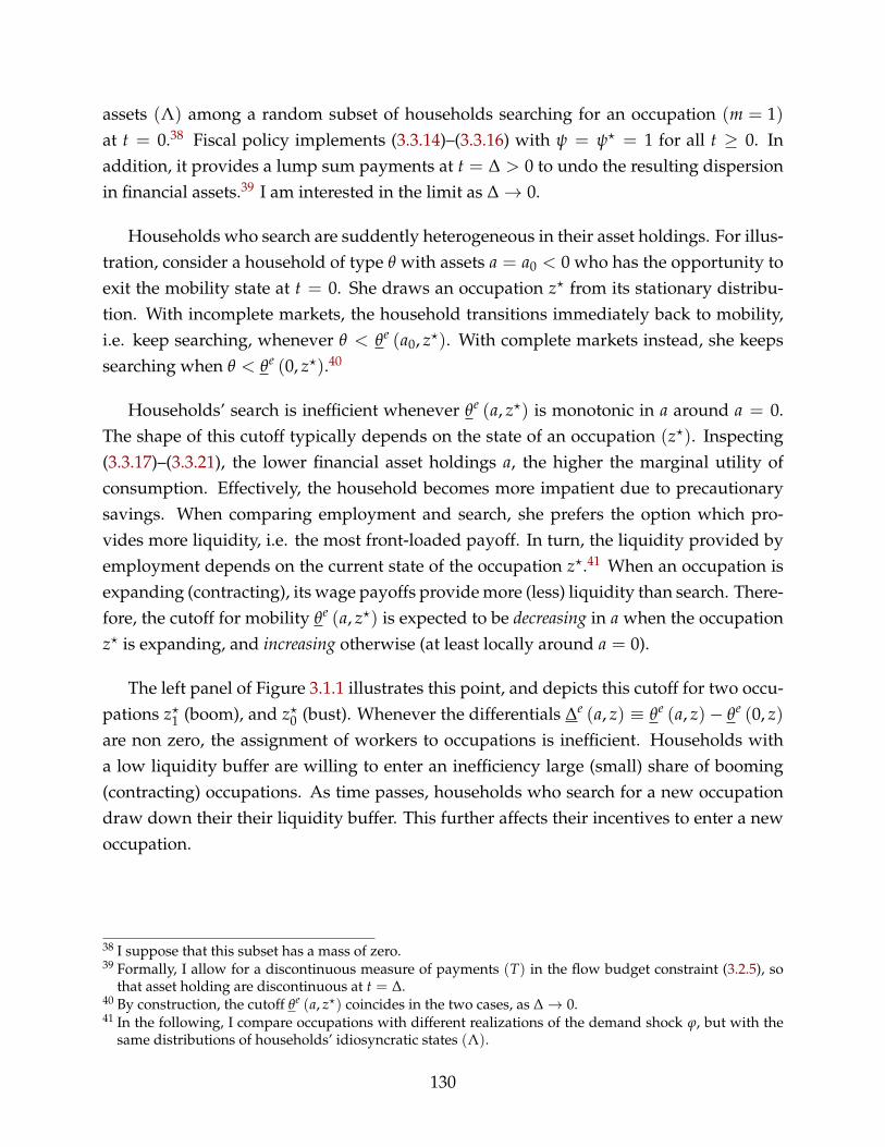
assets (Λ) among a random subset of households searching for an occupation (m = 1)at t = 0.38 Fiscal policy implements (3.3.14)–(3.3.16) with ψ = ψ? = 1 for all t ≥ 0. Inaddition, it provides a lump sum payments at t = ∆ > 0 to undo the resulting dispersionin financial assets.39 I am interested in the limit as ∆ → 0.

Households who search are suddently heterogeneous in their asset holdings. For illus-tration, consider a household of type θ with assets a = a0 < 0 who has the opportunity toexit the mobility state at t = 0. She draws an occupation z? from its stationary distribu-tion. With incomplete markets, the household transitions immediately back to mobility,i.e. keep searching, whenever θ < θe (a0, z?). With complete markets instead, she keepssearching when θ < θe (0, z?).40

Households’ search is inefficient whenever θe (a, z?) is monotonic in a around a = 0.The shape of this cutoff typically depends on the state of an occupation (z?). Inspecting(3.3.17)–(3.3.21), the lower financial asset holdings a, the higher the marginal utility ofconsumption. Effectively, the household becomes more impatient due to precautionarysavings. When comparing employment and search, she prefers the option which pro-vides more liquidity, i.e. the most front-loaded payoff. In turn, the liquidity provided byemployment depends on the current state of the occupation z?.41 When an occupation isexpanding (contracting), its wage payoffs provide more (less) liquidity than search. There-fore, the cutoff for mobility θe (a, z?) is expected to be decreasing in a when the occupationz? is expanding, and increasing otherwise (at least locally around a = 0).

The left panel of Figure 3.1.1 illustrates this point, and depicts this cutoff for two occu-pations z?1 (boom), and z?0 (bust). Whenever the differentials ∆e (a, z) ≡ θe (a, z)− θe (0, z)are non zero, the assignment of workers to occupations is inefficient. Households witha low liquidity buffer are willing to enter an inefficiency large (small) share of booming(contracting) occupations. As time passes, households who search for a new occupationdraw down their their liquidity buffer. This further affects their incentives to enter a newoccupation.

38 I suppose that this subset has a mass of zero.39 Formally, I allow for a discontinuous measure of payments (T) in the flow budget constraint (3.2.5), so

that asset holding are discontinuous at t = ∆.40 By construction, the cutoff θe (a, z?) coincides in the two cases, as ∆ → 0.41 In the following, I compare occupations with different realizations of the demand shock ϕ, but with the

same distributions of households’ idiosyncratic states (Λ).

130

Figure 3.3.1: Labor Misallocation

Inefficient Search (ex ante)

a

θ

θe (a, z⋆0 )

θe (a, z⋆1 )

−ϕY 0a0

Δe (a0, z⋆0 )

Δe (a0, z⋆1 )

Inefficient Reallocation (ex post)

a

θ

θm (a, z⋆0 )

−ϕY 0a0

Overall, imperfect risk sharing shortens households’ average job search in this experi-ment whenever ∫

λ0

∫1θ≥θe(a,z?)dg︸︷︷︸

Exit rate with IM

dg′ >∫

λ0

∫1θ≥θe(0,z?)dg︸︷︷︸

Exit rate with CM

dg

and increases its duration otherwise. Here, g and g′ denotes the distribution before andafter, respectively, the mean preserving spread in asset holdings, i.e. with perfect andimperfect risk sharing. Whether unemployment duration is inefficiently long or short de-pends on the exact primitives of my model. This is a quantitative question that I tackle ina richer framework from Section on 3.4. The empirical evidence provides some guidance:Chetty (2008) find that that liquidity frictions shorten the workers’ job search, and Nekoeiand Weber (2017) that they reduce the quality of the resulting matches.

Inefficient reallocation (ex post). The second experiment focuses on household’s decisionto leave their occupation and search for a new one. Their trade-off is similar to the one dis-cussed above, with one exception. Households already located in an occupation (m = 1)have access to rest (χ = r), who those who search (m = 0) do not. This distinction createsa potentially rich pattern of labor reallocation across occupations.

This second experiment consists of one-time, unanticipated reduction in risk sharingfrom ψ = ψ? = 1 to ψ′ = ψ?,′ = 0 in some occupation z? over a period t ∈ [0, ∆) for some∆ > 0. Fiscal policy at t ∈ [∆,+∞) is as described in the previous experiment. Again, Iam interested in the limit as ∆ → 0.

Households are suddently exposed to the demand shocks that hit their occupation.

131

For illustration, I consider a contractionary shock (z?0). Households who are allowed tomove (λ = λ0) choose between two options: being unemployed with income bu over along period of time, or search for a new occupation with income bm and an average tran-sition time 1/λ0. Since bu > bm, moving entails a short-term liquidity cost. Householdstrade-off between this mobility cost and higher continuation value when assigned to anew occupation. Crucially, the associated cutoff for mobility θm (a, z?0) is potentially non-monotonic in its first argument. For sufficiently high holdings of financial assets (a), thiscutoff is expected to be increasing: the lower the asset holdings, the higher the precaution-ary savings motive and the stronger the incentives to search for a better occupation. Forsufficiently low financial asset holdings (a) however, this cutoff is potentially decreasing:the lower the asset holdings, the more prohibitive the liquidity cost of searching for a newoccupation. That is, imperfect risk sharing is responsible for two forces. One induces ex-cess reallocation in downturns among households with low liquidity buffers, as they havea higher marginal utility of improving their (expected) future earnings by moving to an-other occupation. The other commands deficient reallocation, as households are trappedin their activity and unable to pay the liquidity cost to transition to another one.

The right panel of Figure 3.3.1 illustrates this point. Again, I focus on a contractionaryshock (z?0). I depict two possible cutoffs θm (a, z?0). As time passes, households drawdown their their liquidity buffer, and they eventually have the possibility to move be-tween occupations. Households’ pattern of reallocation between occupations depends onthe severity of the contraction (z?0), the payoffs when unemployed and moving betweenoccupations (bu, bm), the expected duration of the transition between occupations (1/λ0),and the share of households who are allowed to move in a given period (s0/s1). Again,whether household’s reallocation is efficient is a quantitative question that I tackle in aricher framework from Section on 3.4.

3.4 A Richer Model

In Section 3.3, I used my benchmark model to clarify how incomplete markets and bor-rowing constraints can hinder the efficient matching between workers and occupations. Inow develop a richer setup to investigate the quantitative importance of the mechanismsI identified. I extend the model along several dimensions. First, I introduce nominalwage rigidities, unvoluntary unemployment and convex labor adjustment costs withinoccupations to obtain more realistic fluctuations in employment at the occupation level.Second, I introduce social insurance in the form of unemployment insurance and sever-ance payments. This allows me to revisit the analysis of Alvarez and Veracierto (2000)

132

and Alvarez and Veracierto (2001) in my setup with occasionally-binding borrowing con-straints. Third, I let the mobility costs λ0 (θ

?) be indexed by the destination occupation,i.e. these costs are occupation-specific. This allows me target to the empirical distributionof employment across occupations and (aggregate) gross flows between sectors.42 Fourth,I suppose that firm’s technologies have decreasing returns. Households use firms’ equityas a precautionary savings buffer. Finally, I introduce worker-specific uninsured idiosyn-cratic productivity shocks to better match the distribution of earnings observed in thedata. I describe the environment below. The full analysis is presented in Zorzi (2020b).

3.4.1 Environment

The environment is identical to the one presented in Section 3.2.1, except for a few changesthat I highlight below.

Occupations. Occupations are now indexed by an extra idiosyncratic state: their stockof (effective) labor (n). The representative firm in each occupation faces convex laboradjustment costs. Let

λ (z?; χ) ≡∫

1χ=χζ? (ξ, θ, θ?)Λ (dz, z?) , χ ∈ e, u

denote the mass of households employed and unemployed in an occupation, respectively.Here, ζ? (ξ, θ, θ?) denotes the effective productivity of households’ unit of labor supply(defined below). The change in the firm’s labor demand is

H (z?) ≡ f−1 (y (z?))− λ (z?; e)

The firm incurs a non-convex labor adjustment cost. It consists of two components. Thefirst one corresponds a discrete severance payment S > 0 to each worker that the firmseparates from.43 The second one takes the form of a convex technological cost

Γ (z?) ≡ κ

∣∣∣∣ H (z?)λ (z?; e)

∣∣∣∣γ (3.4.1)

paid in terms of the final good, for some κ, γ > 0. A mutual fund claims firms’ profits,

42 However, I suppose that these mobility costs not indexed by the occupation of origin. As a result, I cannotmatch empirical gross flows between two occupations.

43 That is, the process for firms’ cumulated payments is discontinuous at the time of separation.

133

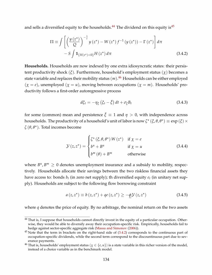
and sells a diversified equity to the households.44 The dividend on this equity is45

Π ≡∫ [(y (z?)

Q

)− 1ν

y (z?)− W (z?) f−1 (y (z?))− Γ (z?)

]dπ

− S∫

1H(z?)<0H (z?) dπ (3.4.2)

Households. Households are now indexed by one extra idiosyncratic states: their persis-tent productivity shock (ξ). Furthermore, household’s employment status (χ) becomes astate variable and replaces their mobility status (m).46 Households can be either employed(χ = e), unemployed (χ = u), moving between occupations (χ = m). Households’ pro-ductivity follows a first-order autoregressive process

dξt = −ηξ

(ξt − ξ

)dt + σξ Bt (3.4.3)

for some (common) mean and persistence ξ ≡ 1 and η > 0, with independence acrosshouseholds. The productivity of a household’s unit of labor is now ζ? (ξ, θ, θ?) ≡ exp (ξ)×ζ (θ, θ?). Total incomes become

𝒴 (z, z?) =

ζ? (ξ, θ, θ?)W (z?) if χ = e

bu + Bu if χ = u

bm (θ) + Bm otherwise

(3.4.4)

where Bu, Bm ≥ 0 denotes unemployment insurance and a subsidy to mobility, respec-tively. Households allocate their savings between the two riskless financial assets theyhave access to: bonds bt (in zero net supply); th diversified equity et (in unitary net sup-ply). Households are subject to the following flow borrowing constraint

a (z, z?) ≡ b (z, z?) + qe (z, z?) ≥ −φ𝒴 (z, z?) (3.4.5)

where q denotes the price of equity. By no arbitrage, the nominal return on the two assets

44 That is, I suppose that households cannot directly invest in the equity of a particular occupation. Other-wise, they would be able to diversify away their occupation-specific risk. Empirically, households fail tohedge against sector-specific aggregate risk (Massa and Simonov (2006)).

45 Note that the term in brackets on the right-hand side of (3.4.2) corresponds to the continuous part ofoccupation-specific dividends, while the second term correspond to the discountinuous part due to sev-erance payments.

46 That is, households’ employment status (χ ∈ e, u) is a state variable in this richer version of the model,instead of a choice variable as in the benchmark model.

134

is equalized (r).47 The households’ flow budget constraint (3.2.5) is

dat (z, z?) = [(1 − τ)𝒴 (z, z?) + rat (z, z?) + T (z, z?)− ct (z, z?)] dt (3.4.6)

where τ denotes a distorsionary tax on incomes.

Labor markets. Labor markets are now subject to search frictions, so that there is unvol-untary unemployment. Nominal wages are sticky and firms face convex labor adjustmentcosts.

The following occurs in period t ≥ 0.48 First, households decide whether to searchwithin their occupation or move to another one (when allowed to), and the firm choosesits labor demand f−1 (y (z?)). Second, some unemployed workers are matched to the firmin their occupation or endogeneous separation occurs, and production occurs. Specifically,if the excess labor demand satisfies H (z?) ≥ 0, i.e. the firm hires, then each unemployedhousehold (χ = u) becomes employed (χ = e) with intensity h (z?; e) ≡ H (z?) /λ (z?; u).Otherwise, i.e. the firm lays off, then each employed household (χ = e) becomes unem-ployed (χ = u) with intensity h (z?; u) ≡ H (z?) /λ (z?; e). Third, exogeneous separationbetween workers and firms takes place with intensity s > 0 in any case. Finally, house-holds who search are (stochastically) assigned to occupations with type-specific intensitiesλ0 (θ

?), and draw a mobility cost as in the benchmark model.

Wage setting. Nominal wages are sticky. Each occupation resets its wage with inten-sity κ > 0. At that point, wages are Nash-bargained (collectively) between the firm andthe households who are present in that occupation. Households have bargaining powerς ∈ (0, 1). The firms’ and households’ threat points are the values of delaying the wagereset until they next have the opportunity to do so. I consider the limit as κ → 0, i.e. wagesare rigid.49 Therefore, wages are only indexed by the occupations’ type: W (z?) = W (θ?)

for some wage schedule W (·).

Market clearing. The good and labor market clearing conditions in each occupation are

y (z?) =∫ ∫

f(

1χ(z)=eζ? (ξ, θ, θ?)Λ (dz, z?))

dπ, (3.4.7)

47 That is, the price of equity satisfies q = rΠ.48 Again, time is continuous so that the exact timing of actions within each mobility state is irrelevant.49 The evidence suggests that wages are very sticky, both for incumbents and new hires (Grigsby et al.

(2019)).

135

The market clearing condition for the final good is50

∫c (z, z?)Λ (dz, z?) dπ =Q +

∫ [bu1χ(z)=u + bm1m=1

]Λ (dz, z?) dπ

+∫

Γ (z?) dπ (3.4.8)

3.4.2 Policy

Fiscal policy. Fiscal policy chooses the level of severance payments S > 0, and financesunemployment insurance and its subsidy to mobility using the distorsionary tax on in-comes. The government’s budget is balanced:∫

τ𝒴 (z, z?)Λ (dz, z?) dg =∫ (

1χ=uBu + 1χ=mBm)

Λ (dz, z?) dg

Monetary policy. Monetary policy sets the nominal interest rate r to implement (uniquely)a non-inflationary, stationary equilibrium for this economy. That is aggregate prices andallocations are constant. The price of the final good is still normalized to 1 (numéraire).

3.4.3 Discussion

Inefficiency. The complete markets allocation is now typically inefficient due to searchfrictions and nominal rigidities. In particular, search frictions contribute to excess unem-ployment compared to the first best allocation. Furthermore, occupation-specific shockslead to an inefficient dispersion in labor market tightness across occupations.51 In thisricher, a new source of inefficiency emerges in general equilibrium. By depressing aggre-gate productivity, labor misallocation lowers the value of firms’ equity below its efficientlevel, i.e. a pecuniary externality. As a result, households hold inefficiently low liquiditybuffers, which makes incomplete markets and borrowing constraints even more acute.

Severance payments. The presence of labor adjustment costs leads to labor hoarding inthis richer model.52 In turn, the effective degree of market incompleteness depends on theimportance of labor hoarding.53 Severance playments (S) play an important role in this

50 The market clearing condition for assets∫ ∫

a (z, z?)Λ (dz, z?) dπ = 1 is redundant.51 Shimer (2007) refers to this inefficient dispersion as “mismatch.” Sahin et al. (2014) assess the importance

of this mismatch to explain the rise is unemployment during the Great Recession.52 Bertola and Caballero (1994) investigate the role of labor hoarding in a Lucas and Prescott (1974) economy

with complete markets.53 Guerrieri et al. (2020) provide an example where, despite incomplete markets, the insurance provided by

labor hoarding allows to implement the complete markets allocation.

136

setup with occasionally-binding borrowing constraints. These payments are fully front-loaded, as opposed to unemployment insurance (Bu) which is claimed linearly over time.Therefore, severance payments allow workers to partially undo the financial frictions thatthey potentially face in the short-term. This effect is absent from earlier work on severancepayments, including Alvarez and Veracierto (2000) and Alvarez and Veracierto (2001).

Job ladder. Workers now search on-the-job even when markets are complete.54 This ef-fectively creates a job-ladder for workers,55 who transition from occupation to occupationuntil they are matched with one where they have a strong comparative advantage. I ex-plore whether workers fall short on climbing their job ladder when markets are incom-plete and workers face borrowing constraints. The presene of on-the-job search allows meto speak to an extensive literature on gross flows across sectors and occupations.56

3.5 Next Steps

In the previous sections, I presented a variant of the Lucas and Prescott (1974) model aug-mented with two-sided heterogeneity between workers and occupations and incompletemarkets. Using this model, I clarified how imperfect risk sharing can hinder the efficientassignment of workers to firms. Taking stock, I presented a quantitative version of thismodel. The next steps consist of calibrating this model to match empirical moments of themicro and aggregate U.S. data, simulate this calibrated model, and solve numerically foroptimal social insurance. The full analysis is presented in Zorzi (2020b).

54 The reason is that I rule out voluntary employment in this richer model.55 Burdett (1978) is a seminal contribution on on-the-job search. Moscarini and Postel-Vinay (2018) provide

a review of the literature on job-ladders.56 Davis and Haltiwanger (1999) survey the evidence on gross flows across occupations and sectors.

Moscarini and Vella (2008) document the cyclical properties of gross flows across occupations.

137



Complete Markets

In this appendix, I state the planner’s problem with complete markets.

Planner’s problem. The planner maximizes

𝒰 ? ≡∫

uθ (c (θ)) dµ

by choosing households’ type-specific consumption c (θ), output of the final sector Q,occupation-specific output y (θ), joint measure g (z?) of households’ idiosyncratic stateswithin each occupation, and the (household) type-specific mass of households g (θ) mov-ing between occupations, and (household) type- and occupation-specific cutoffs for restθr (z?) and mobility θm (z?), subject to the resource constraint∫

c (θ) dµ = Y ≡ Q +∫ [

bu1χ(z)=u + bm1m=1]

Λ (dz, z?) dπ,

the technological constraints

Q =

[∫exp (ϕ)

1ν y (z?)

ν−1ν dπ

] νν−1

andy (z?) = be

∫ ∫1θ≥θr(z?)ζ (θ, θ?)Λ (dz, z?) dg,

together with the restrictions∫ ∫dΛdg +

∫dg = 1 and g, g non-decreasing

139

and the laws of motion for the distributions of households who stay in their occupationand move, respectively. Therefore, the planner’s problem consists of maximizing aggre-gate output Y, subject to the above constraints. The solution to this problem is character-ized in Section 3.3.2.

140


Acemoglu, Daron and David Autor, “Skills, Tasks and Technologies: Implications forEmployment and Earnings,” in O. Ashenfelter and D. Card, eds., Handbook of LaborEconomics, Vol. 4 of Handbook of Labor Economics, Elsevier, 2011, chapter 12, pp. 1043–1171.

and Robert Shimer, “Productivity gains from unemployment insurance,” EuropeanEconomic Review, June 2000, 44 (7), 1195–1224.

Aiyagari, S. Rao, “Uninsured Idiosyncratic Risk and Aggregate Saving,” The QuarterlyJournal of Economics, 1994, 109 (3), 659–684.

Algan, Yann, Olivier Allais, and Wouter J. Den Haan, “Solving heterogeneous-agentmodels with parameterized cross-sectional distributions,” Journal of Economic Dynamicsand Control, March 2008, 32 (3), 875–908.

Alvarez, Fernando and Marcelo Veracierto, “Labor-Market Policies in an EquilibriumSearch Model,” in “NBER Macroeconomics Annual 1999, Volume 14” NBER Chapters,National Bureau of Economic Research, Inc, April 2000, pp. 265–316.

and , “Severance payments in an economy with frictions,” Journal of Monetary Eco-nomics, June 2001, 47 (3), 477–498.

and Robert Shimer, “Search and Rest Unemployment,” Econometrica, January 2011, 79(1), 75–122.

Baqaee, David Rezza and Emmanuel Farhi, “Productivity and Misallocation in GeneralEquilibrium,” The Quarterly Journal of Economics, 2020, 135 (1), 105–163.

Becker, Gary S, “A Theory of Marriage: Part I,” Journal of Political Economy, July-Aug.1973, 81 (4), 813–846.

141

Bertola, Giuseppe and Ricardo J. Caballero, “Cross-Sectional Efficiency and LabourHoarding in a Matching Model of Unemployment,” Review of Economic Studies, 1994,61 (3), 435–456.

Bianchi, Milo and Matteo Bobba, “Liquidity, Risk, and Occupational Choices,” The Re-view of Economic Studies, 10 2012, 80 (2), 491–511.

Blanchard, Olivier and Jordi Galí, “Labor Markets and Monetary Policy: A New Key-nesian Model with Unemployment,” American Economic Journal: Macroeconomics, April2010, 2 (2), 1–30.

Bonin, Holger, Thomas Dohmen, Armin Falk, David Huffman, and Uwe Sunde,“Cross-sectional earnings risk and occupational sorting: The role of risk attitudes,”Labour Economics, December 2007, 14 (6), 926–937.

Burdett, Kenneth, “A Theory of Employee Job Search and Quit Rates,” The American Eco-nomic Review, 1978, 68 (1), 212–220.

Carrillo-Tudela, Carlos and Ludo Visschers, “Unemployment and Endogenous Reallo-cation over the Business Cycle,” ESE Discussion Papers 241, Edinburgh School of Eco-nomics, University of Edinburgh May 2014.

Chang, Yongsung and Sun-Bin Kim, “From Individual To Aggregate Labor Supply: AQuantitative Analysis Based On A Heterogeneous Agent Macroeconomy ,” InternationalEconomic Review, February 2006, 47 (1), 1–27.

Chetty, Raj, “Moral Hazard versus Liquidity and Optimal Unemployment Insurance,”Journal of Political Economy, April 2008, 116 (2), 173–234.

Costinot, Arnaud and Jonathan Vogel, “Beyond Ricardo: Assignment Models in Interna-tional Trade,” Annual Review of Economics, August 2015, 7 (1), 31–62.

Davis, Steven J. and John Haltiwanger, “Gross job flows,” in O. Ashenfelter and D. Card,eds., Handbook of Labor Economics, Vol. 3 of Handbook of Labor Economics, Elsevier, 1999,chapter 41, pp. 2711–2805.

Duffie, Darrell and Larry G Epstein, “Stochastic Differential Utility,” Econometrica, March1992, 60 (2), 353–394.

Dvorkin, Maximiliano and Alexander Monge-Nara, “On the Dynamics of OccupationalChoice, Human Capital Accumulation and Growth,” 2019 Meeting Papers 1461, Societyfor Economic Dynamics 2019.

142

Eeckhout, Jan, “Sorting in the Labor Market,” Annual Review of Economics, August 2018,10 (1), 1–29.

Epstein, Larry G and Stanley E Zin, “Substitution, Risk Aversion, and the Temporal Be-havior of Consumption and Asset Returns: A Theoretical Framework,” Econometrica,July 1989, 57 (4), 937–969.

Evans, David S and Boyan Jovanovic, “An Estimated Model of Entrepreneurial Choiceunder Liquidity Constraints,” Journal of Political Economy, August 1989, 97 (4), 808–827.

Fernández-Villaverde, Jesús, Samuel Hurtado, and Galo Nuño, “Financial Frictions andthe Wealth Distribution,” NBER Working Papers 26302, National Bureau of EconomicResearch, Inc September 2019.

Fuller, David L., Marianna Kudlyak, and Damba Lkhagvasuren, “Productivity insur-ance: The role of unemployment benefits in a multi-sector model,” Journal of EconomicDynamics and Control, 2014, 47 (C), 39–53.

Grigsby, John, Erik Hurst, and Ahu Yildirmaz, “Aggregate Nominal Wage Adjustments:New Evidence from Administrative Payroll Data,” NBER Working Papers 25628, Na-tional Bureau of Economic Research, Inc March 2019.

Guerrieri, Veronica, Guido Lorenzoni, Ludwig Straub, and Iván Werning, “Macroeco-nomic Implications of COVID-19: Can Negative Supply Shocks Cause Demand Short-ages?,” NBER Working Papers 26918, National Bureau of Economic Research, Inc April2020.

Guiso, Luigi and Monica Paiella, “Risk Aversion, Wealth, and Background Risk,” Journalof the European Economic Association, December 2008, 6 (6), 1109–1150.

, Tullio Jappelli, and Luigi Pistaferri, “An Empirical Analysis of Earnings and Employ-ment Risk,” Journal of Business & Economic Statistics, April 2002, 20 (2), 241–253.

Guvenen, Faith, Burhan Kuruscu, Satoshi Tanaka, and David Wiczer, “Multidimen-sional Skill Mismatch,” American Economic Journal: Macroeconomics, January 2020, 12 (1),210–244.

Hsieh, Chang-Tai and Peter J. Klenow, “Misallocation and Manufacturing TFP in Chinaand India,” The Quarterly Journal of Economics, 2009, 124 (4), 1403–1448.

143

Kihlstrom, Richard E and Jean-Jacques Laffont, “A General Equilibrium EntrepreneurialTheory of Firm Formation Based on Risk Aversion,” Journal of Political Economy, August1979, 87 (4), 719–748.

Krusell, Per, Toshihiko Mukoyama, and Aysegül Sahin, “Labour-Market Matching withPrecautionary Savings and Aggregate Fluctuations,” Review of Economic Studies, 2010,77 (4), 1477–1507.

, , Richard Rogerson, and Aysegül Sahin, “Gross Worker Flows over the BusinessCycle,” American Economic Review, November 2017, 107 (11), 3447–3476.

, , , and , “Gross Worker Flows and Fluctuations in the Aggregate Labor Market,”NBER Working Papers 26878, National Bureau of Economic Research, Inc March 2020.

Lindenlaub, Ilse and Fabien Postel-Vinay, “Multidimensional Sorting under RandomSearch,” 2017 Meeting Papers 501, Society for Economic Dynamics 2017.

Lise, Jeremy, Costas Meghir, and Jean-Marc Robin, “Matching, Sorting and Wages,” Re-view of Economic Dynamics, January 2016, 19, 63–87.

Lucas, Robert Jr. and Edward C. Prescott, “Equilibrium search and unemployment,” Jour-nal of Economic Theory, February 1974, 7 (2), 188–209.

Marimon, Ramon and Fabrizio Zilibotti, “Unemployment vs. Mismatch of Talents: Re-considering Unemployment Benefits,” Economic Journal, April 1999, 109 (455), 266–291.

Massa, Massimo and Andrei Simonov, “Hedging, Familiarity and Portfolio Choice,” TheReview of Financial Studies, 01 2006, 19 (2), 633–685.

McLaughlin, Kenneth J and Mark Bils, “Interindustry Mobility and the Cyclical Upgrad-ing of Labor,” Journal of Labor Economics, January 2001, 19 (1), 94–135.

Moscarini, Giuseppe, “Excess Worker Reallocation,” Review of Economic Studies, 2001, 68(3), 593–612.

and Fabien Postel-Vinay, “The Cyclical Job Ladder,” Annual Review of Economics, Au-gust 2018, 10 (1), 165–188.

and Francis G. Vella, “Occupational Mobility and the Business Cycle,” NBER WorkingPapers 13819, National Bureau of Economic Research, Inc February 2008.

Nekoei, Arash and Andrea Weber, “Does Extending Unemployment Benefits ImproveJob Quality?,” American Economic Review, February 2017, 107 (2), 527–561.

144

Postel-Vinay, Fabien and Jeremy Lise, “Multidimensional Skills, Sorting, and HumanCapital Accumulation,” American Economic Review (forthcoming), 2020.

Restuccia, Diego and Richard Rogerson, “Policy Distortions and Aggregate Productivitywith Heterogeneous Plants,” Review of Economic Dynamics, October 2008, 11 (4), 707–720.

Rogerson, Richard, “Sectoral Shocks, Specific Human Capital and Displaced Workers,”Review of Economic Dynamics, January 2005, 8 (1), 89–105.

Sahin, Aysegül, Joseph Song, Giorgio Topa, and Giovanni L. Violante, “Mismatch Un-employment,” American Economic Review, November 2014, 104 (11), 3529–3564.

Schulhofer-Wohl, Sam, “Heterogeneity and Tests of Risk Sharing,” Journal of PoliticalEconomy, 2011, 119 (5), 925–958.

Shimer, Robert, “Mismatch,” American Economic Review, September 2007, 97 (4), 1074–1101.

and Lones Smith, “Assortative Matching and Search,” Econometrica, March 2000, 68(2), 343–370.

Teulings, Coen N. and Pieter A. Gautier, “The Right Man for the Job,” Review of EconomicStudies, 2004, 71 (2), 553–580.

Vereshchagina, Galina and Hugo A. Hopenhayn, “Risk Taking by Entrepreneurs,” Amer-ican Economic Review, December 2009, 99 (5), 1808–1830.

Zorzi, Nathan, “Investment Dynamics and Cyclical Redistribution,” Mimeo, MIT April2020.

, “Uninsured Income Risk and Labor Misallocation,” In Progress, MIT May 2020.

145

Nathan Gaspar Zorzi

Documents

Transcript of Nathan Gaspar Zorzi